Model Diagnostics Based on Cumulative Residuals: The R-package gof

The case of generalized linear models was first examined by Su and Wei (1991). Let $Y$ be the response variable with a distribution from a (natural) exponential family:

parameterized by $\theta$ (and the dispersion parameter $\phi$) and the known functions $a,b$ and $c$. Direct calculations reveals that the

The mean $\mathbb{E}{Y_{i}}=\mu(\theta_{i})$ is related to some covariates, $\bm{x}_{i}$, through a link-function (McCullagh and Nelder, 1983), $g$,

i.e., $\theta_{i}=\theta_{i}(\bm{\beta})$. Typically, the canonical link is chosen such that $g\circ\mu=\id$, with the most common regression models being the general linear model, logistic regression and Poisson regression

Given $n$ observations $(y_{i},x_{1i},\ldots,x_{pi})_{i=1,\ldots,n}$ the maximum likelihood estimate $\widehat{\bm{\beta}}\in\mathbb{R}^{p}$ is obtained by solving the set of score equations:

with $h=\partial\{(g\circ\mu)^{-1}\}$. We define the (raw) residuals $e_{i}=y_{i}-g^{-1}(\widehat{\bm{\beta}}^{T}\bm{x}_{i})$, $i=1,\ldots,n$. Our interest is the cumulative sum of the residuals over the $j$th covariate (Su and Wei, 1991; Lin et al., 2002):

In contrast to the distribution of individual residuals, we can determine the distribution (under the null) of this aggregate. For known parameters the asymptotics can be derived as a Brownian bridge (Shorack and Wellner, 1986), however, we need to take uncertainty in estimation of $\widehat{\bm{\beta}}$ into account. Under certain regularity conditions, a Taylor expansion around the true parameter value, $\bm{\beta}_{0}$, gives us

Let $\mathcal{I}(\widehat{\bm{\beta}})=\mathbb{E}(-\nabla U(\widehat{\bm{\beta}}))$ denote the Fisher information. Now $(\widehat{\bm{\beta}}-\bm{\beta}_{0})$ is asymptotically normally distributed and asymptotically equivalent with $\mathcal{I}(\widehat{\bm{\beta}})^{-1}U(\widehat{\bm{\beta}})$:

It then follows that the process

with i.i.d. $G_{1},\ldots,G_{n}\sim\mathcal{N}(0,1)$, $i=1,\ldots,n$, and

(see Table 1) converges weakly to the same limiting distribution as the observed process (5) (Lin et al., 2002).

To test the functional form of the $j$th covariate we look at a Kolmogorov-Smirnov (KS) type supremum statistic:

Alternatively tests can be based on the Cramer-von-Mises (CvM) functional:

A large number of realizations of $\widehat{W}_{j}$ is generated. The supremum statistic is calculated for each realization and the p-value is estimated from the empirical distribution of these statistics. The residuals can also be cumulated after the predicted values (Lin et al., 2002)

which leads to a test of misspecified link function.

The linear structural equation models covers a broad range of models including the general linear model, path analysis and various latent variable models. Diagnostics based on cumulative residuals was examined in this case by Sánchez et al. (2009) building on the work of Pan and Lin (2005) on Generalized Linear Mixed Models (GLMM) sharing many of the aspects of structural equation models. The basic idea and proof of weak convergence is very similar to the case of GLM.

A structural equation model is typically divided into two separate parts. For the $i$th individual we have a measurement part describing the multivariate outcome $\bm{Y}_{i}$:

where $\bm{\eta}_{i}$ are the latent variables and $\bm{X}_{i}$ are covariates, and a structural part describing the latent variables:

where $\bm{\nu}\in\mathbb{R}^{p}$, $\bm{\Lambda}\in\mathbb{R}^{p\times l}$, $\bm{K}\in\mathbb{R}^{p\times q}$, and $\bm{\epsilon}_{i}\sim\mathcal{N}_{p}(0,\bm{\Sigma_{\epsilon}})$. And $\bm{\alpha}\in\mathbb{R}^{l}$, $\bm{B}\in\mathbb{R}^{l\times l}$, $\bm{\Gamma}\in\mathbb{R}^{l\times q}$, and $\bm{\zeta}_{i}\sim\mathcal{N}(0,\bm{\Psi})$. Hence, the model is parameterized by some $\bm{\theta}$ defining $(\bm{\nu},\bm{\alpha},\bm{\Lambda},\bm{K},\bm{B},\bm{\Gamma},\bm{\Sigma_{\epsilon}},$ $\bm{\Psi})$ with some restrictions to guarantee identification. The conditional moments of $\bm{Y}_{i}$ given $\bm{X}_{i}$, are

and inference on $\bm{\theta}$ is usually obtained by MLE Bollen (1989).

The residuals can be predicted as the conditional mean given the endogenous variables and covariates. Hence,

where $\bm{\pi}_{r}^{s}\colon\mathbb{R}^{s}\to\mathbb{R}$ is the projection onto coordinate $s$. Different local aspects of the structural equation model can now be assessed by examining the cumulative residual processes of either $\widehat{\epsilon}_{ik}$ and $\widehat{\zeta}_{ig}$.

Misspecified covariate effect on the $g$th latent variable is checked by summing $\widehat{\zeta}_{ig}$ with respect to the $j$th covariate, $(X_{ij})$:

and as for the GLM we can imitate the behavior of this process under the null of no misspecification by simulation. Misspecified link between $g$th latent variable and its predictors is checked by summing $\widehat{\zeta}_{ig}$ with respect to $\mathbb{E}(\eta_{ig}\mid\bm{X_{i}})=\bm{\pi}_{g}^{l}(\bm{1}-\bm{B})^{-1}(\bm{\alpha}+\bm{\gamma}\bm{X}_{i})$. To examine departures from the specified association between an endogenous variable and one of its predictors, we can look at the cumulative process defined by summing $\widehat{\epsilon}_{ik}$ with respect to $X_{j}$ or $\mathbb{E}(\eta_{ig}\mid\bm{X}_{i})$. This can also be used to diagnose for so-called item bias (conditional dependence between a covariate and endogenous variable given latent variables). Finally, misspecified link between an endogenous variable and its linear predictors is checked by summing $\widehat{\epsilon}_{ik}$ with respect to $\mathbb{E}(Y_{ik}\mid\bm{X}_{i})$.

The idea of looking at aggregates of residuals can also be applied as a tool for diagnosing the proportional hazards assumptions used in many survival analyses. We will assume that we have triplet observations $(N_{i}(t),$ $Y_{i}(t),$ $X_{i}(t)),$ $i=1,\ldots,n$ of a counting process, at-risk process and covariate process in the compact time-interval $[0,\tau]$. Using the notation of stochastic integrals we let the Martingale decomposition of the counting process be given by

Cox’s proportional hazard model assumes intensity takes the form

where $X$ is $p$-dimensional covariates. We denote the cumulative baseline hazard

As the model contains a non-parametric term, $\lambda_{0}$, inference will be based on the partial likelihood (Cox, 1972)

where

with the first and second partial derivatives

and let $E(t,\beta)=S_{1}/S_{0}(t,\beta)$. The score equation then becomes

The Nelson-Aalen estimator of the cumulative intensity is

where $N_{.}=\sum_{i}N_{i}$. Define

and hence minus the derivative of the score is $I(\tau,\beta)$ (i.e., the information). The estimated martingales residual process is given by

(with the martingale residuals defined by evaluation in $\tau$), and the estimated score process

where $X_{i}(s)-E(s,\widehat{\beta})$ are the Schoenfeld residuals.

To assess the proportional hazards assumption we will calculate the Kolmogorov-Smirnov and Cramer-von-Mises test statistics of the different coordinates of the observed score process. As in the previous section we can simulate realizations under the null (proportional hazards). The key result is that $n^{-1/2}\widehat{U}(\widehat{\beta},t)$ is asymptotically equivalent to

with

where $e(t,\beta_{0})\overset{\mathbb{P}}{=}\lim_{n\to\infty}E(t,\beta_{0})$ (see (Martinussen and Scheike, 2006; Lin et al., 1993)), which follows from a Taylor expansion around the true parameter $\beta_{0}$. With the estimates plugged in we get

Given observed times $(T_{1},\ldots,T_{n})$ and death-indicators $\Delta_{i}$, ($X_{i}=X_{i}(T_{i})$) we can implement this by

Finally $n^{-1/2}M_{1i}(t)$ is asymptotically equivalent to $n^{-1/2}\sum_{i=1}^{n}\widehat{M}_{1i}(t)G_{i}$ where the $G_{i}$’s are i.i.d. $\mathcal{N}(0,1)$.

The described methods are implemented in the R-package gof available from the Comprehensive R Archive Network (R Core Team, 2012).

The package has been designed to work directly on lm, glm and coxph objects (Therneau and original R port by Thomas Lumley, 2013). Additionally, various aspects of latent variable models, fitted via the lava-package (Holst and Budtz-Joergensen, 2012), can be diagnosed.

The simulation routine is computational intensive and to obtain better computing efficiency, the resampling routines was written in C++. The implementation uses the Scythe Statistical Library (Pemstein et al., 2011) which among other things offers operator overloaded matrix operations making the (linear) algebraic computations in the program close to self-documenting.

First we define a simple function that allows us to simulate data from Binomial and Poisson regression models with link function $g$, and covariates $X,Z\sim\mathcal{N}(0,1)$

R> sim1 <- function(n,f=sum,family=binomial("logit")) { x <- rnorm(n) z <- rnorm(n) if (is.character(family)) family <- do.call(family,list()) eta <- family$linkinv(apply(cbind(x,z),1,f)) y <- switch(family$family, binomial= (eta>runif(n))*1, poisson= rpois(n,eta), eta) return(data.frame(y,x,z)) }

We first simulate binomially distributed observations and use a complementary log-log link:

R> d <- sim1(n=1000,family=binomial("cloglog"))Next we fit both the correct model and the model with canonical link

R> l1 <- glm(y˜x+z,d,family=binomial("cloglog"))R> l2 <- glm(y˜x+z,d,family=binomial("logit"))Using the cumres method, we calculate the cumulative residual process ordered by the predicted values and simulate 1,000 processes from the null

R> library("gof")

R> (g1 <- cumres(l1,R=1000,variable="predicted"))

Kolmogorov-Smirnov-test: p-value=0.466Cramer von Mises-test: p-value=0.333Based on 1000 realizations. Cumulated residuals ordered by predicted-variable.---

Kolmogorov-Smirnov-test: p-value=0.466Cramer von Mises-test: p-value=0.333Based on 1000 realizations. Cumulated residuals ordered by predicted-variable.---

R> (g2 <- cumres(l2,R=1000,variable="predicted"))

Kolmogorov-Smirnov-test: p-value=0.014Cramer von Mises-test: p-value=0Based on 1000 realizations. Cumulated residuals ordered by predicted-variable.---

Kolmogorov-Smirnov-test: p-value=0.014Cramer von Mises-test: p-value=0Based on 1000 realizations. Cumulated residuals ordered by predicted-variable.---There are clear indications, by both the supremum and CvM test, of misspecification of the link function in model l2. To plot the observed process and realizations from under the null (the number of realization can be changed in the cumres call with the argument plots), we can use the plot method

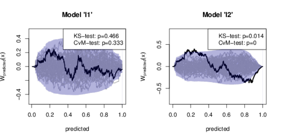
It is evident from the plot (Figure ), that the observed process of model 2 is extreme.

Next we simulate data from a Poisson regression model

R> d2 <- sim1(200,f=function(x) 0.5*x[1]ˆ2+x[2],family=poisson())and we fit a Poisson regression model but with misspecified functional form of the covariate $X$

R> l <- glm(y˜x+z,family=poisson(),data=d2)Next we check the link function and functional form of both covariates

R> (g <- cumres(l,R=2000))

Kolmogorov-Smirnov-test: p-value=0.453Cramer von Mises-test: p-value=0.547Based on 2000 realizations. Cumulated residuals ordered by predicted-variable.---Kolmogorov-Smirnov-test: p-value=0.001Cramer von Mises-test: p-value=0Based on 2000 realizations. Cumulated residuals ordered by x-variable.---Kolmogorov-Smirnov-test: p-value=0.8185Cramer von Mises-test: p-value=0.858Based on 2000 realizations. Cumulated residuals ordered by z-variable.---

Kolmogorov-Smirnov-test: p-value=0.453Cramer von Mises-test: p-value=0.547Based on 2000 realizations. Cumulated residuals ordered by predicted-variable.---Kolmogorov-Smirnov-test: p-value=0.001Cramer von Mises-test: p-value=0Based on 2000 realizations. Cumulated residuals ordered by x-variable.---Kolmogorov-Smirnov-test: p-value=0.8185Cramer von Mises-test: p-value=0.858Based on 2000 realizations. Cumulated residuals ordered by z-variable.---and we plot all processes (Figure 2) while changing the color (and alpha blending) of the realizations and prediction-band (setting col or col.ci to NULL will disable either the realizations or the prediction-band)

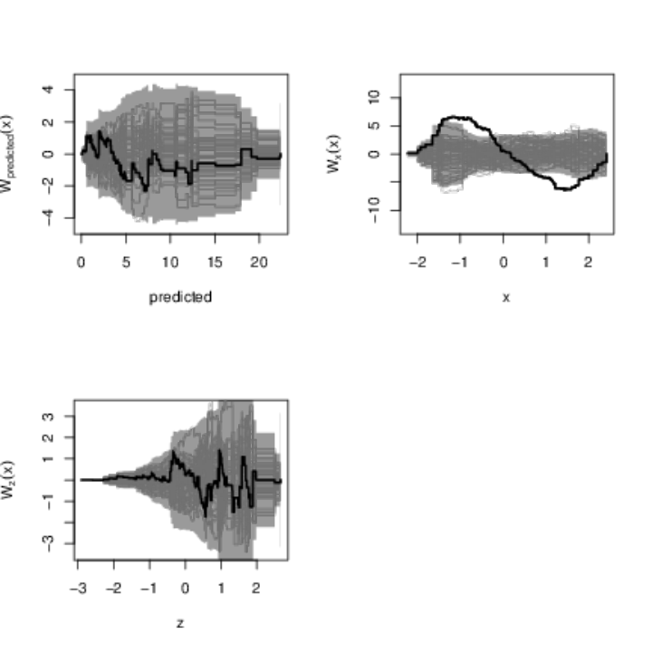
Again, the misspecification (of the functional form of $X$) is evident from the plots.

The cumres method is also available for structural equation models fitted via the lava package (Holst and Budtz-Joergensen, 2012). As an example we will examine a simple model, with three outcomes described by the equation

with $i=1,\ldots,n$ individuals and latent variable $\eta_{i}$. We also add a structural equation describing the latent variable

with covariates $X$ and $Z1$. The residual terms $\epsilon_{i1},\ldots,\epsilon_{i3},\zeta$ are normally distributed and independent. In lava we can specify the model as

R> library(lava)R> m <- lvm(list(c(y1,y2,y3)˜eta,eta˜x+z))R> latent(m) <- ˜etaWe simulate 200 observations from a structural equation model like the one defined above, with intercepts set to zero and all other parameters equal to one, but with

R> m0 <- mR> functional(m0,y2˜eta) <- function(x) xˆ2R> functional(m0,eta˜z) <- function(x) x+0.5*xˆ2R> d <- sim(m0,200)Next we find the MLE of the first model

R> (e <- estimate(m,d))

Estimate Std. Error Z-value P-valueMeasurements: y2<-eta 2.21830 0.24535 9.04147 <1e-12 y3<-eta 0.99314 0.05380 18.45847 <1e-12Regressions: eta<-x 1.00280 0.09820 10.21176 <1e-12 eta<-z 1.08055 0.09790 11.03729 <1e-12Intercepts: y2 2.84517 0.48757 5.83545 5.365e-09 y3 -0.05982 0.09412 -0.63558 0.5251 eta 0.50307 0.10623 4.73553 2.185e-06Residual Variances: y1 0.67836 0.15287 4.43739 y2 40.57804 4.22914 9.59488 y3 0.92828 0.16468 5.63682 eta 1.57358 0.21605 7.28351and as an example we cumulate the predicted residual terms of $Y_{3}$ and $Y_{2}$ against $\mathbb{E}(\eta_{i}\mid X_{i})$, and the residual term of $\eta_{i}$ against the two covariates.

R> e.gof <- cumres(e,list(y3˜eta,y2˜eta,eta˜x,eta˜z),R=1000)From the cumulative residual plots (see Figure 3) we clearly see the misspecification in the measurement model of the second outcome (with the observed process also indicating a quadratic form), and also the wrongly specified functional form of $X$.

For complete flexibility the cumres method can be used with the syntax cumres(model,y,x,...), where y is a function of the model parameters returning the residuals of interest, and x can be any vector to order the residuals by. Typically y will be defined via the predict method of a lvmfit object (a lava model object).

As an example of checking the proportional hazards assumption in a Cox model, we will analyze the Mayo Clinic PBC data. Dickson et al. (1989) suggested a Cox model for analyzing the survival of the liver disease patient with 5 covariates: age, edema status, logarithmic serum bilirubin, logarithmic standardized blood clotting time, and logarithmic serum albumin:

R> library("survival")R> data("pbc")R> pbc.cox <- coxph(Surv(time,status==2)˜age+edema+log(bili)+ log(protime)+log(albumin), data=pbc)

To check the proportional hazards assumption, we examine the score process vs. follow-up time:

R> pbc.gof <- cumres(pbc.cox,R=2000)and plot the observed process with realizations from the null

There are clear indication of violation of the proportional hazards assumption for blood clotting time (protime), and indication of problems with the edema variable. To remedy the non-proportionality, time-varying covariate effects could be introduced to the model, e.g.,

R> library("timereg")R> pbc.caalen <- cox.aalen(Surv(time,status==2) ˜ prop(age) + prop(edema) + prop(bili) + protime, data=pbc, n.sim=500)

References

- Bollen (1989) Bollen, K. A., 1989. Structural equations with latent variables. Wiley Series in Probability and Mathematical Statistics: Applied Probability and Statistics. John Wiley & Sons Inc., New York, a Wiley-Interscience Publication.
- Cox (1972) Cox, D. R., 1972. Regression models and life tables. J. Roy. Stat. Soc. Ser. B 34, 406–424.
- Dickson et al. (1989) Dickson, E., Grambsch, P., Fleming, T., Fisher, L., Langworthy, A., 1989. Prognosis in primary biliary cirrhosis: model for decision making. Hepatology 10, 1–7.
- Holst and Budtz-Joergensen (2012) Holst, K. K., Budtz-Joergensen, E., 2012. Linear latent variable models: The lava-package. Computational StatisticsHttp://dx.doi.org/10.1007/s00180-012-0344-y.
- Lin et al. (1993) Lin, D. Y., Wei, L. J., Ying, Z., 1993. Checking the Cox model with cumulative sums of martingale-based residuals. Biometrika 80 (3), 557–572.
- Lin et al. (2002) Lin, D. Y., Wei, L. J., Ying, Z., 2002. Model-Checking Techniques Based on Cumulative Residuals. Biometrics 58, 1–12.
- Martinussen and Scheike (2006) Martinussen, T., Scheike, T. H., 2006. Dynamic regression models for survival data. Statistics for Biology and Health. Springer-Verlag, New York.
- McCullagh and Nelder (1983) McCullagh, P., Nelder, J. A., 1983. Generalized linear models. Monographs on Statistics and Applied Probability. Chapman & Hall, London.
- Pan and Lin (2005) Pan, Z., Lin, D. Y., 2005. Goodness-of-fit methods for generalized linear mixed models. Biometrics 61, 1000–1009.
- Pemstein et al. (2011)
Pemstein, D., Quinn, K. M., Martin, A. D., 6 2011. The scythe statistical
library: An open source c++ library for statistical computation. Journal of
Statistical Software 42 (12), 1–26.
URL http://www.jstatsoft.org/v42/i12 - R Core Team (2012)
R Core Team, 2012. R: A Language and Environment for Statistical Computing. R
Foundation for Statistical Computing, Vienna, Austria, ISBN 3-900051-07-0.
URL http://www.R-project.org - Sánchez et al. (2009) Sánchez, B. N., Houseman, E. A., Ryan, L. M., 2009. Residual-based diagnostics for structural equation models. Biometrics 65 (1), 104–115.
- Shorack and Wellner (1986) Shorack, G. R., Wellner, J. A., 1986. Empirical Processes with Applications to Statistics. John Wiley & Sons, New York.
- Su and Wei (1991) Su, J. Q., Wei, L. J., 1991. A lack-of-fit test for the mean function in a generalized linear model. Journal of American Statistical Association 86 (414), 420–426.
- Therneau and original R port by Thomas Lumley (2013)
Therneau, T., original R port by Thomas Lumley, 2013. survival: Survival
analysis, including penalised likelihood. R package version 2.37-4.
URL http://CRAN.R-project.org/package=survival - Zeileis (2006)
Zeileis, A., 2006. Object-oriented computation of sandwich estimators. Journal
of Statistical Software 16 (9), 1–16.
URL http://www.jstatsoft.org/v16/i09/.