Searching for Vector Dark Matter via Higgs Portal at the LHC

This section briefly introduces the WIMP model and discusses the relevant interactions with DM candidates. For studying the minimal extension of the SM that incorporates DM, besides the SM particles and their associated gauge symmetry, we consider a new local $SU(2)_{X}$ gauge symmetry and add one quadruplet of $SU(2)_{X}$ to the model. Thus, the Lagrangian in $SU(2)_{X}\times SU(2)_{L}\times U(1)_{Y}$ is written as:

with

where ${\cal L}_{SM}$ is the Lagrangian of the SM, $H^{T}=(G^{+},(v+\phi+iG^{0})/\sqrt{2})$ is the SM Higgs doublet, $\Phi^{T}_{4}=(\phi_{3/2},\phi_{1/2},-\phi_{-1/2},\phi_{-3/2})/\sqrt{2}$ is the quadruplet of $SU(2)_{X}$, the index $i$ of $\phi_{i}$ stands for the eigenvalue of the third generator of $SU(2)_{X}$, and $\phi_{-i}=\phi^{*}_{i}$. The covariant derivative of $\Phi_{4}$ is $D_{\mu}=\partial_{\mu}+ig_{X}T^{a}X^{a}_{\mu}$ and the representations of $T^{3}$ is given by $T^{3}={\rm diag}(3/2,1/2,-1/2,-3/2)$. The $T^{1,2}$ can be found elsewhere [32]. Since the SM is well known, it is not presented here explicitly.

For breaking the $SU(2)_{X}$ and preserving a discrete symmetry, the non-vanishing VEV and the associated fields that fluctuate around the VEV are set to:

With the breaking pattern in Eq. (3), one can find that an $Z_{3}$ symmetry $U_{3}\equiv e^{iT^{3}4\pi/3}={\rm diag}(1,e^{i2\pi/3},e^{-2i\pi/3},1)$ is preserved by the ground state $\Phi_{0}=(v_{4}/2,0,0,v_{4}/2)$. Under $Z_{3}$ transformation, the scalar fields of the quadruplet are transformed as:

That is, $\phi_{\pm 3/2}$ are $Z_{3}$-blind while $\phi_{\pm 1/2}$ carry the charge of $Z_{3}$. In terms of the physical states of gauge fields, one can write:

with $T^{\pm}=T^{1}\pm iT^{2}$ and $\chi_{\mu}(\bar{\chi}_{\mu})=(X^{1}_{\mu}\mp iX^{2}_{\mu})/\sqrt{2}$, where $\bar{\chi}_{\mu}$ is regarded as the antiparticle of $\chi_{\mu}$. The transformations of gauge fields are [32]:

It can be seen that $\phi_{\pm 1/2}$ and $\chi_{\mu}(\bar{\chi}_{\mu})$ carry the charges of $Z_{3}$. Since the masses of $\chi_{\mu}$ and $\bar{\chi}_{\mu}$ arise from the spontaneous symmetry breaking of $\Phi_{4}$. $\phi_{\pm 1/2}$ must be the Nambu-Goldstone bosons and are the longitudinal degrees of freedom of $\chi_{\mu}$ and $\bar{\chi}_{\mu}$. Hence, $\chi_{\mu}$ and $\bar{\chi}_{\mu}$ are the candidates of DM in the model.

In this section, we discuss the new free parameters and their relationships. The new free parameters only appear in the new gauge sector and scalar potential shown in Eq. (2). They are $g_{X}$, $\mu^{2}_{\Phi}$, $\lambda_{\Phi}$, and $\lambda^{\prime}$. In terms of the SM Higgs doublet and quadruplet of $SU(2)_{X}$ and the scalar potential, the mass matrix for SM Higgs $\phi$ and new scalar $\phi_{r}$ is expressed as:

with $m_{\phi}=\sqrt{2\lambda}v$ and $m_{\phi_{r}}=\sqrt{2\lambda_{\Phi}}v_{4}$. Clearly, $\lambda^{\prime}$ causes the mixture of Higgs doublet $H$ and quadruplet $\Phi_{4}$. The mixing angle connecting the mass eigenstates can be parametrized as:

where $h$ denotes the SM-like Higgs boson, $H^{0}$ is the second scalar boson and $\tan 2\theta=2\lambda^{\prime}vv_{4}/(m^{2}_{\phi_{r}}-m^{2}_{\phi})$. According to Eq. (II.2), the eigenvalues of the mass square matrix are found as:

We note that the mass of $h$ can be larger or less than that of $H^{0}$. In addition, from the kinetic term of $\Phi_{4}$, the masses of gauge bosons can be obtained as $m_{\chi}=\sqrt{3}g_{X}v_{4}/2$ and $m_{X^{3}}=\sqrt{3}m_{\chi}$. Hence, the set of new free parameters can be chosen as:

The mixing angle $\theta$ is constrained by the Higgs boson search at the LEP and the LHC. A thorough analysis [46] has provided the constraint as a function of the second scalar boson mass. The constraints are taken into account in the analysis of discovery significance below.

Next, we discuss the couplings of DM in the model. Since the DM candidates are the gauge bosons, their couplings to the visible sector are through the mixture of $SU(2)_{X}$ quadruplet and the SM Higgs doublet. Therefore, the main interactions of DM are from the kinetic term of $\Phi_{4}$. With the mixing angle defined in Eq. (II.2), the relevant interactions are given as [32]:

with $c_{\theta}=\cos\theta$ and $s_{\theta}=\sin\theta$. With these interactions, it can be seen that if $m_{h}>2m_{\chi}$, then the invisible Higgs decay $h\to\chi\bar{\chi}$ will give a strict limit on $\sin\theta$. Besides the gauge interactions, we also derive the triple scalar couplings, expressed as:

Since the mixing angle $\theta$ is related to the parameter $\lambda^{\prime}$, the two terms in each triple interaction should be the same in terms of their order of magnitude. If the mixing angle is not suppressed, $H^{0}$ with $m_{H^{0}}>m_{h}/2$ or $m_{H^{0}}<m_{h}/2$ through the decay $H^{0}\to hh$ or $h\to H^{0}H^{0}$ has an interesting effect on the production of DM. However, since the mixing angle is constrained by DM direct detection and the effects of triple couplings on the production of DM pairs are small, we will not further discuss their contributions in this paper.

By Eq. (19), we see that the vector DM candidates only couple to SM Higgs $h$ and new scalar $H^{0}$. For producing a pair of DM particles, $h$ and $H^{0}$ could be both off-shell and on-shell. For the off-shell case, the effect is directly related to the magnitude of couplings and the main constraints are from DM relic density and DM direct detection. For the on-shell case, besides the constraints mentioned above, the invisible Higgs decay also gives a strong bound. For presenting the constraint from the invisible Higgs decay, we formulate the partial decay rate for $h(H^{0})\to\chi\chi$ with $m_{h(H^{0})}>m_{\chi}/2$ as:

where $g^{\prime}=g_{X}s_{\theta}(g_{X}c_{\theta})$ when $S=h(H^{0})$. The branching ratios (BRs) of the invisible decays can be expressed as:

with $\Gamma_{h\to{\rm SM}}$ being the width of the SM Higgs. The expression of $\Gamma_{h\to{\rm SM}}^{m_{H^{0}}}$ is the same as that of $\Gamma_{h\to SM}$ but $m_{h}$ is replaced by $m_{H^{0}}$.

According to the observations of ATLAS [30] and CMS [31], the Higgs mass now is known to be $m_{h}=125$ GeV and the associated width is $\Gamma_{h\to SM}=4.21$ MeV [47]. Taking these values as inputs, we plot the contours for BR($h\to\chi\chi$) as a function of $g_{X}\tan\theta$ and $m_{\chi}$ in left panel of Fig. 1, where the solid line denotes the current upper limit of data with $BR(h\to\chi\chi)<0.29$ [48] and the region above the curve is excluded. Although the new scalar boson $H^{0}$ has not been observed yet and its mass is unknown, for completeness, we also show its invisible decay as a function of $g_{X}\cot\theta$ and $m_{\chi}$ in the right panel of Fig. 1 with the setting of $m_{H^{0}}=2m_{\chi}+1$ GeV, where the adopted mass relation $m_{H^{0}}\simeq 2m_{\chi}$ can explain the galactic center gamma-ray excess [32].

Based on a previous investigation [32], it is known that the measured relic density of DM could bound the couplings of DM annihilating into SM particles; however, a stronger limit has arisen from the direct detection. By Eq. (19), we see that the coupling of each $h$ and $H^{0}$ to $\chi$ is associated with $s_{\theta}$ and $c_{\theta}$, respectively. Since their couplings to quarks are $c_{\theta}$ and $s_{\theta}$, except the mass differences of intermedia, the spin-independent cross section of DM scattering off nucleons only depends on $g_{X}c_{\theta}s_{\theta}$ for both $h$ and $H^{0}$. In terms of the results measured by the LUX Collaboration [2], we present the allowed values of $g_{X}s_{\theta}$ and $m_{X}$ in Fig. 2, where the dashed and dotted lines stand for $m_{H^{0}}=m_{\chi}$ and $2m_{\chi}$, respectively. For comparison, we also show the situation for invisible Higgs decay $h\to\chi\bar{\chi}$. From the results, it can be seen that for $m_{\chi}<m_{h(H^{0})}/2$, invisible Higgs decay gives the most restrictive limit. However, for $m_{H^{0}}\sim m_{\chi}$, the strongest bound is from the experiment of DM direct detection.

The signals of WIMPs in the model originate from the SM Higgs and new scalar $H^{0}$ decays, denoted by $S^{(*)}\to\chi\bar{\chi}$, in which scalar $S$ can be on-shell or off-shell. The potential channels for producing DM pairs through the $S$-portal are found to be (a) VBF, $pp\to S^{(*)}jj$, (b) mono jet, $pp\to S^{(*)}j$, (c) mono W/Z, $pp\to S^{(*)}W/Z$, and (d) $t\bar{t}$, $pp\to S^{(*)}t\bar{t}$. The mono jet is the loop-induced process $gg\to S^{(*)}g$ [49, 50]. In order to understand and estimate the production cross section of each channel, we implemented our model in CalcHEP [51] and utilized the code with CTEQ6L PDF [52] and $\sqrt{s}=14$ TeV to run numerical calculations.

Consequently, the production cross sections for $pp\to S^{(*)}X$, with X being the involved final state, are presented in Fig. 3, where the left panel is for on-shell $H^{0}$. Since the effect of on-shell $h$ is similar to that of $H^{0}$, except for $c_{\theta}$ dependence instead of $s_{\theta}$, here we only show the results of $H^{0}$. The right panel of Fig. 3 is for off-shell $h$ and $H^{0}$. In this case, since $m_{\chi}$ and $m_{H^{0}}$ are the explicit parameters in the processes, we adopt $m_{H^{0}}=m_{\chi}$ as the representative case. For reducing the dependence of this parameter, we scale the left and right panels by factors of $1/s^{2}_{\theta}$ and $1/(g^{2}_{X}s^{2}_{\theta}c^{2}_{\theta})$, respectively. From these results, it can be clearly seen that mono jet and VBF processes dominate the production cross section in the region of $m_{H^{0}}>50$ GeV. Nevertheless, when we further impose the kinematic cuts for reducing the events of backgrounds, the contributions of mono jet to the significance will become sub-leading effects. Hence, the main contributions to the signals are indeed from the VBF process and thus we focus our study on this channel. Additionally, from the plots, we also know that the off-shell processes are much smaller than those arising from the resonance of $S$.

Since DM candidates are invisible particles and the production mechanism at the LHC in the model is through VBF, the signal events at the detector level will appear as:

where $\not{E}_{T}$ is the missing transverse energy. As known, the background events generated from the SM contributions can also mimic the signal events of Eq. (24). In order to distinguish the signals from the backgrounds, we consider the following background processes [53]:
(1) $Zjj$ background : $pp\to Zjj$ ,
(2) $Zjjj$ background : $pp\to Zjjj$ ,
(3) $Wjj$ background : $pp\to W^{\pm}jj$,
(4) $Wjjj$ background : $pp\to W^{\pm}jjj$,
(5) top background : $pp\to tW^{-}\bar{b}(\bar{t}W^{+}b)$,
where the missing transverse energy $\not{E}_{T}$ is from the $Z$- and $W$-boson leptonic decays. Although charged leptons can be generated by $W$ decays, when they are misidentified by the detectors, the events will appear as missing $E_{T}$. Similarly, this situation could also happen in jet. Therefore, for analyzing the backgrounds, when the events are generated, we set the number of jets in the final states to be up to three. We note that although QCD multi jets are also the source of background, however their contributions can be further reduced by the kinematic cuts.

For enhancing the ratio of the signal to background, we propose proper criteria to suppress the backgrounds. Since Higgs portal DM production at the LHC has been studied in the literature [59, 60] and the production mechanism also exists in our model, we first perform the DM production through the processes $pp\to hqq$ and invisible Higgs decay $h\to\chi\bar{\chi}$. Then, we can directly apply the event selections for invisible Higgs search proposed by CMS [43] and set them as

where $p_{T}(j)$ and $\eta(j)$ are the transverse momentum and pseudo-rapidity of jet $j$, and $M_{jj}$ is the invariant mass of two jets. Although these conditions are used for collision energy at $\sqrt{s}=7$ and 8 TeV in the CMS experiments, according to our MG5 event simulations, it is found that the distributions of jet $p_{T}$ and $\not{E}_{T}$ indeed are not sensitive to the total collision energy of LHC. Therefore, in this study we take these selection conditions as the basic criteria for event kinematic cuts at $\sqrt{s}=14$ TeV. Using the event generator MG5 and the cuts of Eq. (25), we show the histograms of the signal and background as a function of ${\not{E}}_{T}$, $\Delta\eta_{jj}$, $M_{jj}$ and $\Delta\phi_{jj}$ in Figs. 4(a), (b), (c), and (d), respectively, where $\Delta\eta_{jj}=|\eta_{j_{1}}-\eta_{j_{2}}|$ and $\Delta\phi_{jj}=|\phi_{j_{1}}-\phi_{j_{2}}|$ are the pseudo-rapidity difference and azimuthal angle difference of the two-jet final state, respectively.

From the results of Fig. 4, we find that at low $\Delta\eta_{jj}$, background events are much larger than signals. If we further impose a cut on $\Delta\eta_{jj}$, the background events will be significantly reduced. Similar behavior also occurs at $M_{jj}<1100$ GeV and $\Delta\phi_{jj}>1.5$. Therefore, utilizing the difference in the kinematic region between the signal and background, we propose stricter event selection conditions on $\Delta\eta_{jj}$, $M_{jj}$, and $\Delta\phi_{jj}$, given as:

When both cuts of Eqs. (25) and (26) are imposed simultaneously, the resultant histograms as a function of ${\not{E}}_{T}$, $\Delta\eta_{jj}$, $M_{jj}$, and $\Delta\phi_{jj}$ are shown in Fig. 5.

The event production of $pp\to S^{(*)}(\to\chi\bar{\chi})X$ depends on the mass of DM. For interpreting the gamma-ray excess from the galactic center at the same time, we concentrate on the DM with $m_{\chi}<m_{W}$. For distinguishing the contributions of on-shell $h$ from the off-shell one, we set the allowed range of $m_{\chi}$ to be the following two schemes:

where the former dictates DM pair production to be through invisible Higgs decay while the latter dictates it to be through the Higgs propagator. Based on a previous study [32], for explaining the galactic center gamma-ray excess via DM annihilation in this model, the favored ranges for $m_{H^{0}}$ are $m_{H^{0}}\gtrsim 2m_{\chi}$ and $m_{H^{0}}\lesssim m_{\chi}$. In order to fit well with gamma-ray data, we find $m_{H^{0}}\sim 2m_{\chi}$ and $m_{\chi}\sim m_{H^{0}}$. For numerical calculations, we adopt the mass relation as:

Here, $H^{0}$ can decay into a DM pair in case ${\rm A}$ while case ${\rm B}$ is through off-shell $H^{0}$. Since $m_{h}=125$ GeV is known and the unobserved $m_{H^{0}}$ is still a free parameter, we investigate various situations by combining schemes ${\rm I}$ and ${\rm II}$ of Eq. (27) with cases $A$ and $B$ of Eq. (28), denoted as $\rm I_{A}$, $\rm I_{B}$, $\rm II_{A}$, and $\rm II_{B}$,

After setting up the kinematic cuts and classifying the possible schemes for $m_{\chi}$ and $m_{H^{0}}$, we calculate the cross sections of the background and signal with various values of $m_{\chi}$ in schemes $\rm I_{A,B}$ and $\rm II_{A,B}$. The numerical values are presented in Table 1, where the simulated events had passed through ${\tt PYTHIA\,6}$ and ${\tt PGS\,4}$ detector simulation, the cuts of Eqs. (25) and (26) were employed, $R_{h}=c^{2}_{\theta}BR(h\to\chi\bar{\chi})$, $R_{H^{0}}=s^{2}_{\theta}BR(H^{0}\to\chi\bar{\chi})$, and $R_{\rm off}=(g_{X}s_{\theta}c_{\theta})^{2}$. The associated cross section is obtained as:

Here, $\sigma^{\rm MG5}_{BG/S}$ is the cross section of the background/signal provided by MG5, $N_{\rm tot}$ is the number of original generated events and $N_{\rm cuts}$ is the number of selected events. For the background events, we have summed up all channels. We find that the dominant backgrounds are from $Z$ + jets, where $Z$ invisibly decays into neutrinos. By requiring null charged leptons in the final states, the event number from $W$ + jets should be smaller than that from $Z$ + jets. We also investigate the background associated with the top-quark by generating event $tW^{-}\bar{b}(\bar{t}W^{+}b)$, which includes $t\bar{t}$ production. Since the corresponding cross section is less than 1 fb when event selections are applied, we do not show its value in Table. 1. To understand the effect of kinematical cuts, we show the background cross section for each step of cuts, where the basic cuts are shown in Eq. (25). It can be clearly seen that $\Delta\eta_{jj}$ cuts reduce the background significantly.

For studying the potentiality of discovery, as typically done, we define the significance as $S=n_{s}/\sqrt{n_{b}}$, where $n_{s}$ and $n_{b}$ denote the numbers of selected events for the signal and background, respectively. For numerical illustration, we take $m_{\chi}=50$ GeV for the schemes $\rm I_{A,B}$ and $m_{\chi}=70$ GeV for schemes ${\rm II_{A,B}}$. Here, we adopt $m_{H}=m_{\chi}-1$ GeV and $m_{H}=2m_{\chi}+1$ GeV for schemes ${\rm\{I_{B},II_{B}\}}$ and ${\rm\{I_{A},II_{A}\}}$, respectively. Accordingly, we display the discovery significance as a function of $g_{X}s_{\theta}$ with 100 and 300 fb^-1 in Fig. 6. Since the sensitive regions of $g_{X}s_{\theta}$ are different in different schemes, we take the horizontal domain to be $[0.002,0.02$], $[0.05,0.2]$, and $[0.3,3]$ for ${\rm I_{A,B}}$, ${\rm II_{A}}$ and ${\rm II_{B}}$, respectively.

For understanding the influence of $g_{X}$, we show the situations of $g_{X}=(0.05,1.0)$ for scheme $I_{A}$ and $g_{X}=(0.5,1.0)$ for scheme ${\rm II_{A}}$. From the plots, it can be seen that when the value of $g_{X}s_{\theta}$ is fixed, the contributions of $H^{0}$ are smaller in schemes ${\rm I_{A}}$ if the value of $g_{X}$ is larger. That is, $H^{0}$ in ${\rm I_{A}}$ has a significant effect at small $g_{X}$ or large $s_{\theta}$ values. Since $H^{0}$ is off-shell in scheme ${\rm I_{B}}$ and its effect is negligible, by comparing the results of ${\rm I_{A}}$ with those of ${\rm I_{B}}$, one can determine the influence of on-shell $H^{0}$ on ${\rm I_{A}}$. Since $h$ is an off-shell particle in scheme ${\rm II_{A}}$, the main contributions are from the invisible $H^{0}$ decays. According to Eq. (23) and the results of Fig. 1 and Table 1, we need a somewhat larger value of $g_{X}s_{\theta}$ to get more signal events. Therefore, the domain of $g_{X}s_{\theta}$ is set to be one order of magnitude larger than that in ${\rm I_{A,B}}$. In scheme ${\rm II_{B}}$, the signal events are from off-shell $h$ and $H^{0}$. Therefore, in order to enhance the signal events, we need a large value of $g_{X}s_{\theta}$. Unfortunately, when $S>2$, $g_{X}$ becomes a strong coupling constant. We thus omit the scheme ${\rm II_{B}}$ in the following discussions.

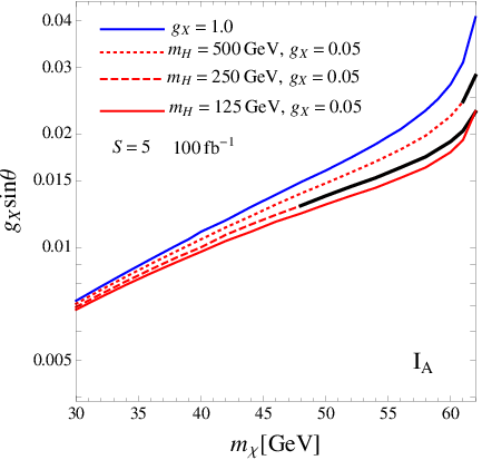
Furthermore, in order to understand the dependence of significance on the second Higgs mass, we investigate the significance by changing the value of $m_{H}$. We note that scheme ${\rm I_{B}}$ is independent of $m_{H}$ as long as it satisfies $m_{H}<2m_{\chi}$ because off-shell $H^{0}$ effects are negligible. We thus focus on schemes ${\rm I_{A}}$ and ${\rm II_{A}}$ here. The upper left (right) plot in Fig. 7 shows the contours in $m_{\chi}$-$g_{X}\sin\theta$ plane with $S=2(5)$. For $g_{X}=0.05$, we take $m_{H}=125$, $250$ and $500$ GeV. Due to the small $\sin\theta$, $H^{0}$ contributions are negligible and the $g_{X}=1$ case does not depend on $m_{H}$ . It can be seen that if the value of $g_{X}\sin\theta$ is fixed, the significance increases with decreasing $m_{H}$. Moreover the effect of $H^{0}$ can be seen for $2m_{\chi}\sim m_{h}$, even though $m_{H}$ is as heavy as 500 GeV. Also, the region with thick black lines is excluded from the analysis of the Higgs boson search at the LHC in Fig. 4 of Ref. [46]. The lower plot in Fig. 7 show the contours in the $m_{H}$-$\sin\theta$ plane with $S=2$ and 5. Since the branching ratio for $H^{0}\to\chi\bar{\chi}$ is $\sim 1$, the significance in scheme ${\rm II_{A}}$ does not strongly depend on $g_{X}$ when $g_{X}\gtrsim 0.1$. Moreover the significance does not depend on $m_{\chi}$ as long as $m_{H}>2m_{\chi}$ is satisfied. We also show the upper limit of $\sin\theta$, taken from Fig. 4 of Ref. [46], as a function of $m_{H}$. We find that the stronger constraint for $\sin\theta$ is in the higher $m_{H}$ region.

After studying the potential for discovering DM signatures at the LHC, in order to further understand the relationship between significance and free parameters, we show the correlation between $g_{X}s_{\theta}$ and $m_{\chi}$ for schemes ${\rm I_{A,B}}$ and ${\rm II_{A}}$ in Fig. 8. Since the significance in the situation of lower $m_{H}$ and on-shell $H^{0}$ is larger, we also consider $m_{H}=2m_{\chi}+1$ GeV for schemes ${\rm I_{A}}$ and ${\rm II_{A}}$. For illustration, we use 100 fb^-1 and adopt $S=2$ and $S=5$ in the plots. Since the large $g_{X}s_{\theta}$ in scheme ${\rm II_{B}}$ is excluded by DM direct detection experiments, we do not further discuss the case. Additionally, the limit obtained from DM direct detection is also shown in the plots.

From the results in Fig. 8, it can be seen that the current invisible Higgs decay measured by ATLAS at $\sqrt{s}=8$ TeV [48] cannot give a strict bound on the parameters of schemes ${\rm I_{A}}$ and ${\rm I_{B}}$. Due to off-shell $h$, the data of invisible Higgs decay are not suitable for scheme ${\rm II_{A}}$. Recalling the results in Fig. 2, since the constraint from invisible Higgs decay in scheme ${\rm I_{A}(I_{B})}$ is stronger (weaker) than that from the LUX experiment, the significance over $S=2$ with 100 fb^-1 in scheme ${\rm I_{B}}$ is excluded by the current LUX data. For enhancing the significance of scheme ${\rm I_{B}}$, a higher luminosity is necessary. Although the required values of $g_{X}s_{\theta}$ for $S=5$ in scheme ${\rm II_{A}}$ are one order of magnitude larger than those in scheme ${\rm I_{B}}$, for the case with $m_{H^{0}}=2m_{\chi}+1>m_{h}$, $S=5$ is still allowed, even though the limit of the LUX is considered. We conclude that schemes ${\rm I_{A}}$ and ${\rm II_{A}}$ have the highest discovery potential in our model.

References

- [1] K. A. Olive et al. (Particle Data Group), Chin. Phys. C, 38, 090001 (2014).
- [2] D.S. Akerib et al. [LUX Collaboration], arXiv:1310.8214 [astro-ph.CO].
- [3] O. Adriani et al. [PAMELA Collaboration], Nature 458, 607 (2009) [arXiv:0810.4995 [astro-ph]].
- [4] M. Ackermann et al. [Fermi LAT Collaboration], Phys. Rev. Lett. 108, 011103 (2012) [arXiv:1109.0521 [astro-ph.HE]].
- [5] L. Accardo et al. [AMS Collaboration], Phys. Rev. Lett. 113, 121101 (2014).
- [6] M. Aguilar et al. [AMS Collaboration], Phys. Rev. Lett. 113, 221102 (2014).
- [7] D. Hooper, P. Blasi and P. D. Serpico, JCAP 0901, 025 (2009) [arXiv:0810.1527]; H. Yuksel, M. D. Kistler and T. Stanev, Phys. Rev. Lett. 103, 051101 (2009) [arXiv:0810.2784 [astro-ph]]; S. Profumo, Central Eur. J. Phys. 10, 1 (2011) [arXiv:0812.4457 [astro-ph]]; D. Malyshev, I. Cholis and J. Gelfand, Phys. Rev. D 80, 063005 (2009) [arXiv:0903.1310 [astro-ph.HE]].
- [8] D. Grasso et al. [FERMI-LAT Collaboration], Astropart. Phys. 32 (2009) 140 [arXiv:0905.0636 [astro-ph.HE]]; T. Linden and S. Profumo, Astrophys. J. 772, 18 (2013) [arXiv:1304.1791 [astro-ph.HE]]; P. -F. Yin, Z. -H. Yu, Q. Yuan and X. -J. Bi, Phys. Rev. D 88, no. 2, 023001 (2013) [arXiv:1304.4128 [astro-ph.HE]].
- [9] K. Blum, B. Katz and E. Waxman, Phys. Rev. Lett. 111, no. 21, 211101 (2013) [arXiv:1305.1324 [astro-ph.HE]].
- [10] L. Goodenough and D. Hooper, arXiv:0910.2998 [hep-ph].
- [11] D. Hooper and L. Goodenough, Phys. Lett. B 697, 412 (2011) [arXiv:1010.2752 [hep-ph]].
- [12] A. Boyarsky, D. Malyshev and O. Ruchayskiy, Phys. Lett. B 705, 165 (2011) [arXiv:1012.5839 [hep-ph]].
- [13] D. Hooper and T. Linden, Phys. Rev. D 84, 123005 (2011) [arXiv:1110.0006 [astro-ph.HE]].
- [14] K. N. Abazajian and M. Kaplinghat, Phys. Rev. D 86, 083511 (2012) [Erratum-ibid. D 87, 129902 (2013)] [arXiv:1207.6047 [astro-ph.HE]].
- [15] C. Gordon and O. Macias, Phys. Rev. D 88, no. 8, 083521 (2013) [Erratum-ibid. D 89, no. 4, 049901 (2014)] [arXiv:1306.5725 [astro-ph.HE]].
- [16] O. Macias and C. Gordon, Phys. Rev. D 89, no. 6, 063515 (2014) [arXiv:1312.6671 [astro-ph.HE]].
- [17] K. N. Abazajian, N. Canac, S. Horiuchi and M. Kaplinghat, Phys. Rev. D 90, no. 2, 023526 (2014) [arXiv:1402.4090 [astro-ph.HE]].
- [18] V. Vitale et al. [Fermi/LAT Collaboration], arXiv:0912.3828 [astro-ph.HE].
- [19] A. Morselli et al. [Fermi-LAT Collaboration], Nuovo Cim. C 034N3, 311 (2011) [arXiv:1012.2292 [astro-ph.HE]].
- [20] T. Daylan, D. P. Finkbeiner, D. Hooper, T. Linden, S. K. N. Portillo, N. L. Rodd and T. R. Slatyer, arXiv:1402.6703 [astro-ph.HE].
- [21] B. Zhou, Y. F. Liang, X. Huang, X. Li, Y. Z. Fan, L. Feng and J. Chang, arXiv:1406.6948 [astro-ph.HE].
- [22] F. Calore, I. Cholis and C. Weniger, arXiv:1409.0042 [astro-ph.CO].
- [23] K. N. Abazajian, N. Canac, S. Horiuchi, M. Kaplinghat and A. Kwa, arXiv:1410.6168 [astro-ph.HE].
- [24] F. Calore, I. Cholis, C. McCabe and C. Weniger, arXiv:1411.4647 [hep-ph].
- [25] J. D. Ruiz-Alvarez, C. A. de S.Pires, F. S. Queiroz, D. Restrepo and P. S. Rodrigues da Silva, Phys. Rev. D 86, 075011 (2012) [arXiv:1206.5779 [hep-ph]].
- [26] Y. Farzan and A. R. Akbarieh, JCAP 1210, 026 (2012) [arXiv:1207.4272 [hep-ph]].
- [27] A. Alves, S. Profumo, F. S. Queiroz and W. Shepherd, Phys. Rev. D 90, no. 11, 115003 (2014) [arXiv:1403.5027 [hep-ph]].
- [28] A. Berlin, P. Gratia, D. Hooper and S. D. McDermott, Phys. Rev. D 90, 015032 (2014) [arXiv:1405.5204 [hep-ph]].
- [29] B. Patt and F. Wilczek, hep-ph/0605188.
- [30] G. Aad et al. [ATLAS Collaboration], Phys. Lett. B 716, 1 (2012) [arXiv:1207.7214 [hep-ex]].
- [31] S. Chatrchyan et al. [CMS Collaboration], Phys. Lett. B 716, 30 (2012) [arXiv:1207.7235 [hep-ex]].
- [32] C. H. Chen and T. Nomura, Phys. Lett. B 746, 351 (2015) [arXiv:1501.07413 [hep-ph]].
- [33] T. Hambye, JHEP 0901, 028 (2009) [arXiv:0811.0172 [hep-ph]].
- [34] C. W. Chiang, T. Nomura and J. Tandean, JHEP 1401, 183 (2014) [arXiv:1306.0882 [hep-ph]].
- [35] C. Boehm, M. J. Dolan and C. McCabe, Phys. Rev. D 90, no. 2, 023531 (2014) [arXiv:1404.4977 [hep-ph]].
- [36] V. V. Khoze and G. Ro, JHEP 1410, 61 (2014) [arXiv:1406.2291 [hep-ph]].
- [37] S. Baek, P. Ko and W. I. Park, JCAP 1410, 067 (2014) [arXiv:1311.1035 [hep-ph]].
- [38] C. Gross, O. Lebedev and Y. Mambrini, arXiv:1505.07480 [hep-ph].
- [39] S. Di Chiara and K. Tuominen, arXiv:1506.03285 [hep-ph].
- [40] G. Belanger, B. Dumont, U. Ellwanger, J. F. Gunion and S. Kraml, Phys. Lett. B 723, 340 (2013) [arXiv:1302.5694 [hep-ph]].
- [41] A. Greljo, J. Julio, J. F. Kamenik, C. Smith and J. Zupan, JHEP 1311, 190 (2013) [arXiv:1309.3561 [hep-ph]].
- [42] G. Aad et al. [ATLAS Collaboration], Phys. Rev. Lett. 112, 201802 (2014) [arXiv:1402.3244 [hep-ex]].
- [43] S. Chatrchyan et al. [CMS Collaboration], Eur. Phys. J. C 74, 2980 (2014) [arXiv:1404.1344 [hep-ex]].
- [44] M. Endo and Y. Takaesu, Phys. Lett. B 743, 228 (2015) [arXiv:1407.6882 [hep-ph]].
- [45] N. Craig, H. K. Lou, M. McCullough and A. Thalapillil, arXiv:1412.0258 [hep-ph].
- [46] T. Robens and T. Stefaniak, Eur. Phys. J. C 75, 104 (2015) [arXiv:1501.02234 [hep-ph]].
- [47] S. Heinemeyer et al. [LHC Higgs Cross Section Working Group Collaboration], arXiv:1307.1347 [hep-ph].
- [48] The ATLAS collaboration, ATLAS-CONF-2015-004, ATLAS-COM-CONF-2015-004.
- [49] J. Goodman, M. Ibe, A. Rajaraman, W. Shepherd, T. M. P. Tait and H. B. Yu, Phys. Rev. D 82, 116010 (2010) [arXiv:1008.1783 [hep-ph]].
- [50] P. J. Fox, R. Harnik, J. Kopp and Y. Tsai, Phys. Rev. D 85, 056011 (2012) [arXiv:1109.4398 [hep-ph]].
- [51] A. Belyaev, N. D. Christensen and A. Pukhov, Comput. Phys. Commun. 184, 1729 (2013) [arXiv:1207.6082 [hep-ph]].
- [52] P. M. Nadolsky, H. L. Lai, Q. H. Cao, J. Huston, J. Pumplin, D. Stump, W. K. Tung and C.-P. Yuan, Phys. Rev. D 78, 013004 (2008) [arXiv:0802.0007 [hep-ph]].
- [53] D. Ghosh, R. Godbole, M. Guchait, K. Mohan and D. Sengupta, Phys. Lett. B 725, 344 (2013) [arXiv:1211.7015 [hep-ph]].
- [54] J. Alwall, R. Frederix, S. Frixione, V. Hirschi, F. Maltoni, O. Mattelaer, H.-S. Shao and T. Stelzer et al., JHEP 1407, 079 (2014) [arXiv:1405.0301 [hep-ph]].
- [55] C. S. Deans [NNPDF Collaboration], arXiv:1304.2781 [hep-ph].
- [56] A. Alloul, N. D. Christensen, C. Degrande, C. Duhr and B. Fuks, Comput. Phys. Commun. 185, 2250 (2014) [arXiv:1310.1921 [hep-ph]].
- [57] T. Sjostrand, S. Mrenna, P. Z. Skands, JHEP 0605 , 026 (2006).
- [58] http://www.physics.ucdavis.edu/~conway/research/software/pgs/pgs4-general.htm.
- [59] A. Djouadi, O. Lebedev, Y. Mambrini and J. Quevillon, Phys. Lett. B 709, 65 (2012) [arXiv:1112.3299 [hep-ph]].
- [60] A. Djouadi, A. Falkowski, Y. Mambrini and J. Quevillon, Eur. Phys. J. C 73, no. 6, 2455 (2013) [arXiv:1205.3169 [hep-ph]].