跳到论文正文
W Papers独立论文阅读器 arXiv:1507.00812 论文正文 计算阅读时间 · 0%
引用这篇论文根据当前论文元数据生成,正式投稿前建议核对。


License: arXiv.org perpetual non-exclusive license
arXiv:1507.00812v1 [gr-qc] 03 Jul 2015

Removing Ostrogradski’s ghost from cosmological perturbations in f⁡(R,Rμ​ν2,Cμ​ν​ρ​σ2)f(R,R_{\mu\nu}^{2},C_{\mu\nu\rho\sigma}^{2}) gravity

Preprint: RUP-15-15
Yuji Akita Affiliation: Department of Physics, Rikkyo University, Toshima, Tokyo 175-8501, Japan    Tsutomu Kobayashi Affiliation: Department of Physics, Rikkyo University, Toshima, Tokyo 175-8501, Japan
Abstract

Recently it was argued that gravity with the squire of the Ricci tensor can be stabilized by adding constraints to the theory. This was so far demonstrated for fluctuations on the Minkowski/de Sitter background. We show that the same scheme works equally well for removing Ostrogradski’s ghost from fluctuations on a cosmological background in generic f⁡(R,Rμ​ν2,Cμ​ν​ρ​σ2)f(R,R_{\mu\nu}^{2},C_{\mu\nu\rho\sigma}^{2})-type theories of gravity. We also derive the general formula for the spectrum of primordial tensor perturbations from the stabilized theory.

pacs
04.50.Kd

I Introduction

Physical laws describing the time evolution are written in the form of differential equations up to second order in time. This is indeed the case for classical mechanics, Maxwell’s theory of electromagnetism, and general relativity. Then, what if one has the evolution equations of higher order in time? The answer is tragic; one will encounter Ostrogradski’s ghost that is the generic instability in non-degenerate higher derivative theories [1, 2, 3]. Ostrogradski’s instability can be illustrated by the following simple example [4]:

S=∫d​t​[12​q¨2−V⁡(q)].\displaystyle S=\int{\rm d}t\left[\frac{1}{2}\ddot{q}^{2}-V(q)\right]. (1)

This action yields the fourth-order equation of motion for qq. Defining the canonical coordinates Q1:=qQ_{1}:=q, Q2:=q˙Q_{2}:=\dot{q} and their conjugate momenta P1P_{1}, P2P_{2}, one obtains the Hamiltonian,

H=P1​Q2+P222+V⁡(Q1).\displaystyle H=P_{1}Q_{2}+\frac{P_{2}^{2}}{2}+V(Q_{1}). (2)

This Hamiltonian linearly depends on P1P_{1} and hence is not bounded from below, signaling the instability.

General relativity, a second-order theory for the metric, is a healthy theory from this viewpoint. Nevertheless, it is sufficiently reasonable to consider gravitational theories beyond general relativity. Higher powers of the curvature tensors such as R2R^{2} and Rμ​ν​Rμ​νR_{\mu\nu}R^{\mu\nu} are expected to be the low-energy manifestation of quantum gravity. In recent years phenomenological modification of general relativity has been studied extensively in order to account for the present accelerated expansion of the Universe, which involves an arbitrary function of the curvature tensors or a non-minimal coupling to the scalar field. Due to the higher derivative nature, those theories are often plagued by Ostrogradski’s instability.

There are several ways to evade this instability issue. From an effective field theory point of view, if one takes the UV cutoff below the scale at which the ghost emerges then the instability is not necessarily problematic and thus could be circumvented. More directly, one would consider the class of theories that violates the assumptions of Ostrogradski’s theorem. The R2R^{2} model [5] and its f⁡(R)f(R) generalization [6, 7] are degenerate, and hence are free of ghosts. The Galileons [8, 9, 10] and the Horndeski family of scalar-tensor theories [11, 12, 13] have manifestly second-order field equations despite the higher derivative nature of the Lagrangian, and therefore we do not need to care about Ostrogradski’s ghost. (In fact, it is well known that f⁡(R)f(R) theories can be recast in a scalar-tensor theory that is in a subclass of the Horndeski theory.) Recently, an approach in this direction has been pushed forward and healthy theories beyond Horndeski have been developed [14, 15, 16, 17, 18, 19, 20].

Yet another way of getting around the ghost is adding constraints to the theory to reduce the dimensionality of the phase space, as proposed in Refs. [4, 21]. In Ref. [21], the theory described by [22]

S=MPl22​∫d4​x​−g​(R−2​Λ+α​R2+β​Rμ​ν​Rμ​ν)\displaystyle S=\frac{M_{\rm Pl}^{2}}{2}\int{\rm d}^{4}x\sqrt{-g}\left(R-2\Lambda+\alpha R^{2}+\beta R_{\mu\nu}R^{\mu\nu}\right) (3)

was examined. Although this theory contains unstable modes as it is, it can be made stable by the appropriate addition of constraints at least at the level of the quadratic action for fluctuations. This was demonstrated for the fluctuations on the Minkowski and de Sitter backgrounds [21].

The purpose of the present paper is to extend the work of [21]. We consider the more general action of the form

S=∫d4​x​−g​f​(R,Rμ​ν​Rμ​ν,Cμ​ν​ρ​σ​Cμ​ν​ρ​σ),\displaystyle S=\int{\rm d}^{4}x\sqrt{-g}f(R,R_{\mu\nu}R^{\mu\nu},C_{\mu\nu\rho\sigma}C^{\mu\nu\rho\sigma}), (4)

where ff is an arbitrary function, and stabilize the quadratic action for the fluctuations on the Friedmann-Lmaître-Robertson-Walker (FLRW) background. Note that since the Weyl tensor Cμ​ν​ρ​σC_{\mu\nu\rho\sigma} can be expressed in terms of the Riemann tensor, the Ricci tensor, and the Ricci scalar, the above theory is nothing but f⁡(R,Rμ​ν2,Rμ​ν​ρ​σ2)f(R,R_{\mu\nu}^{2},R_{\mu\nu\rho\sigma}^{2}) gravity. This class of gravitational theories has been explored extensively [23, 24, 25, 26, 27, 28, 29, 30]. As an application, we derive the general formula for the primordial power spectrum of the tensor modes from the stabilized action.

The paper is organized as follows. In the next section we give a quick review on the instabilities in f⁡(R,Rμ​ν2,Cμ​ν​ρ​σ2)f(R,R_{\mu\nu}^{2},C_{\mu\nu\rho\sigma}^{2}) gravity. We then stabilize the quadratic action for cosmological perturbations by adding constraints in Sec. III. In Sec. IV, we evaluate the amplitude of primordial tensor modes in the stabilized theory. Section V is devoted to discussion and conclusions.

II Instabilities in f⁡(R,Rμ​ν2,Cμ​ν​ρ​λ2)f(R,R_{\mu\nu}^{2},C_{\mu\nu\rho\lambda}^{2}) gravity

We start with reviewing how ghost instabilities appear in the theory described by the action (4). The background we consider is given by the FLRW metric, d​s2=a2​(η)​(−d​η2+δi​j​d​xi​d​xj){\rm d}s^{2}=a^{2}(\eta)\left(-{\rm d}\eta^{2}+\delta_{ij}{\rm d}x^{i}{\rm d}x^{j}\right). Let us use the notation

r1:=R,r2:=Rμ​ν​Rμ​ν,r3:=Cμ​ν​ρ​σ​Cμ​ν​ρ​σ,\displaystyle r_{1}:=R,\quad r_{2}:=R_{\mu\nu}R^{\mu\nu},\quad r_{3}:=C_{\mu\nu\rho\sigma}C^{\mu\nu\rho\sigma}, (5)

and write f0:=ff_{0}:=f, fi:=∂f/∂rif_{i}:=\partial f/\partial r_{i}, fi​j:=∂2f/∂ri​∂rjf_{ij}:=\partial^{2}f/\partial r_{i}\partial r_{j}, and fi​j​k:=∂3f/∂ri​∂rj​∂rkf_{ijk}:=\partial^{3}f/\partial r_{i}\partial r_{j}\partial r_{k} evaluated at the background, i.e., r1=6​(ℋ2+ℋ′)/a2r_{1}=6\left({\cal H}^{2}+{\cal H}^{\prime}\right)/a^{2}, r2=12​[ℋ4+ℋ2​ℋ′+(ℋ′)2]/a4r_{2}=12\left[{\cal H}^{4}+{\cal H}^{2}{\cal H}^{\prime}+({\cal H}^{\prime})^{2}\right]/a^{4}, and r3=0r_{3}=0, where ℋ:=a′/a{\cal H}:=a^{\prime}/a and the prime denotes differentiation with respect to the conformal time η\eta.

The background equation can be derived simply by substituting the metric d​s2=−N2​(η)​d​η2+a2​(η)​δi​j​d​xi​d​xj{\rm d}s^{2}=-N^{2}(\eta){\rm d}\eta^{2}+a^{2}(\eta)\delta_{ij}{\rm d}x^{i}{\rm d}x^{j} to the action (4), varying it with respect to NN and aa, and then setting N=aN=a. Variation with respect to NN gives

0\displaystyle 0 =\displaystyle= a4​f0−6​a2​ℋ′​f1−12​[(2​f2+3​f11)​ℋ​(2​ℋ3−ℋ′′)+f2​ℋ′​(ℋ2+2​ℋ′)]\displaystyle a^{4}f_{0}-6a^{2}\mathcal{H}^{\prime}f_{1}-12\left[\left(2f_{2}+3f_{11}\right)\mathcal{H}\left(2\mathcal{H}^{3}-\mathcal{H}^{\prime\prime}\right)+f_{2}\mathcal{H}^{\prime}\left(\mathcal{H}^{2}+2\mathcal{H}^{\prime}\right)\right] (6)
−144a2​f12​ℋ​[3​ℋ5−ℋ2​ℋ′′+ℋ​(ℋ′)2+2​ℋ3​ℋ′−2​ℋ′​ℋ′′]\displaystyle-\frac{144}{a^{2}}f_{12}\mathcal{H}\left[3\mathcal{H}^{5}-\mathcal{H}^{2}\mathcal{H}^{\prime\prime}+\mathcal{H}\left(\mathcal{H}^{\prime}\right)^{2}+2\mathcal{H}^{3}\mathcal{H}^{\prime}-2\mathcal{H}^{\prime}\mathcal{H}^{\prime\prime}\right]
−144a4​f22​ℋ​(ℋ2+2​ℋ′)​[4​ℋ5−ℋ2​ℋ′′+2​ℋ​(ℋ′)2−2​ℋ′​ℋ′′].\displaystyle-\frac{144}{a^{4}}f_{22}\mathcal{H}\left(\mathcal{H}^{2}+2\mathcal{H}^{\prime}\right)\left[4\mathcal{H}^{5}-\mathcal{H}^{2}\mathcal{H}^{\prime\prime}+2\mathcal{H}\left(\mathcal{H}^{\prime}\right)^{2}-2\mathcal{H}^{\prime}\mathcal{H}^{\prime\prime}\right].

This equation will be used in the following calculations to eliminate or rearrange some coefficients in the quadratic actions for fluctuations. Variation with respect to aa gives another cumbersome equation which is not used in the present paper.

II.1 Tensor perturbations

Let us first look at Ostrogradski’s instability of tensor perturbations. It is convenient to parametrize the tensor perturbations as

d​s2=a2​[−d​η2+(δi​j+hi​j+12​hi​k​hk​j)​d​xi​d​xj],\displaystyle{\rm d}s^{2}=a^{2}\left[-{\rm d}\eta^{2}+\left(\delta_{ij}+h_{ij}+\frac{1}{2}h_{ik}h_{kj}\right){\rm d}x^{i}{\rm d}x^{j}\right], (7)

as this definition yields −g=a4\sqrt{-g}=a^{4} at quadratic order in fluctuations. Substituting this metric to the action (4), we obtain the quadratic action for the tensor perturbations:

S=∫d4​x\displaystyle S=\int{\rm d}^{4}x {a2f1(14hi​j′2+14hi​j∂2hi​j)+f2​ℋ2(hi​j′2−hi​j∂2hi​j)′\displaystyle\biggl\{a^{2}f_{1}\left(\frac{1}{4}h_{ij}^{\prime 2}+\frac{1}{4}h_{ij}\partial^{2}h_{ij}\right)+\frac{f_{2}{\cal H}}{2}\left(h_{ij}^{\prime 2}-h_{ij}\partial^{2}h_{ij}\right)^{\prime}
+f2[14hi​j′′2−12hi​j′′∂2hi​j+14(∂2hi​j)2+(ℋ2+32ℋ′)hi​j′2+(ℋ2+ℋ′2)hi​j∂2hi​j]\displaystyle+f_{2}\left[\frac{1}{4}h_{ij}^{\prime\prime 2}-\frac{1}{2}h_{ij}^{\prime\prime}\partial^{2}h_{ij}+\frac{1}{4}\left(\partial^{2}h_{ij}\right)^{2}+\left({\cal H}^{2}+\frac{3}{2}{\cal H}^{\prime}\right)h_{ij}^{\prime 2}+\left({\cal H}^{2}+\frac{{\cal H}^{\prime}}{2}\right)h_{ij}\partial^{2}h_{ij}\right]
+f3[12hi​j′′2+hi​j′′∂2hi​j+2hi​j′∂2hi​j′+12(∂2hi​j)2]}.\displaystyle+f_{3}\left[\frac{1}{2}h_{ij}^{\prime\prime 2}+h_{ij}^{\prime\prime}\partial^{2}h_{ij}+2h_{ij}^{\prime}\partial^{2}h_{ij}^{\prime}+\frac{1}{2}\left(\partial^{2}h_{ij}\right)^{2}\right]\biggr\}. (8)

This can be simplified by integration by parts as

S=∫d4x{a28(Ahi​j′2+Chi​j∂2hi​j)+β8[hi​j′′2+2hi​j′∂2hi​j′+(∂2hi​j)2]},\displaystyle S=\int{\rm d}^{4}x\left\{\frac{a^{2}}{8}\left(Ah_{ij}^{\prime 2}+Ch_{ij}\partial^{2}h_{ij}\right)+\frac{\beta}{8}\left[h_{ij}^{\prime\prime 2}+2h_{ij}^{\prime}\partial^{2}h_{ij}^{\prime}+\left(\partial^{2}h_{ij}\right)^{2}\right]\right\}, (9)

where we defined

β:=2​f2+4​f3,\displaystyle\beta:=2f_{2}+4f_{3}, (10)

and

A\displaystyle A :⁣=\displaystyle:= 2​f1+8​f2a2​(ℋ2+ℋ′)−4​f2′​ℋa2,\displaystyle 2f_{1}+\frac{8f_{2}}{a^{2}}\left({\cal H}^{2}+{\cal H}^{\prime}\right)-4f_{2}^{\prime}\frac{{\cal H}}{a^{2}}, (11)
C\displaystyle C :⁣=\displaystyle:= 2​f1+8​f2a2​(ℋ2+ℋ′)+4​f2′a2​ℋ−2a2​(f2′′−2​f3′′).\displaystyle 2f_{1}+\frac{8f_{2}}{a^{2}}\left({\cal H}^{2}+{\cal H}^{\prime}\right)+\frac{4f_{2}^{\prime}}{a^{2}}{\cal H}-\frac{2}{a^{2}}\left(f_{2}^{\prime\prime}-2f_{3}^{\prime\prime}\right). (12)

Throughout the paper we assume that β=β⁡(η)\beta=\beta(\eta) never vanishes.11 1 If ff depends on the curvature invariants through the Gauss-Bonnet combination, 𝒢:=Rμ​ν​ρ​λ2−4​Rμ​ν2+R2{\cal G}:=R_{\mu\nu\rho\lambda}^{2}-4R_{\mu\nu}^{2}+R^{2}, i.e., f=f⁡(R,𝒢)f=f(R,{\cal G}), we identically have β=0\beta=0. Therefore, we do not consider the f⁡(R,𝒢)f(R,{\cal G}) class of theories in this paper. Linear cosmological perturbations are healthy in f⁡(R,𝒢)f(R,{\cal G}) gravity [31], though it was found in the end that ghost degrees of freedom cannot be avoided on less symmetric backgrounds [32]. The resultant action turns out to be of the same form as that on the Minkowski/de Sitter background in the α​R2+β​Rμ​ν​Rμ​ν\alpha R^{2}+\beta R_{\mu\nu}R^{\mu\nu} theory [21], though in the present case the coefficients AA, CC, and β\beta are time-dependent in general. The quadratic action (9) contains higher derivative terms, and hence Ostrogradski’s instability appears as expected.

We confirm the presence of Ostrogradski’s instability in a more rigorous way by the Hamiltonian analysis. Defining the canonical coordinates as

hi​j≡hi​j\displaystyle h_{ij}\equiv h_{ij} ⟷\displaystyle\longleftrightarrow πi​j=14​[a2​A​hi​j′−β⁡(hi​j′′′−2​∂2hi​j′)−β′​hi​j′′],\displaystyle\pi^{ij}=\frac{1}{4}\left[a^{2}Ah_{ij}^{\prime}-\beta\left(h_{ij}^{\prime\prime\prime}-2\partial^{2}h_{ij}^{\prime}\right)-\beta^{\prime}h_{ij}^{\prime\prime}\right]~, (13)
qi​j≡hi​j′\displaystyle q_{ij}\equiv h_{ij}^{\prime} ⟷\displaystyle\longleftrightarrow pi​j=β4​hi​j′′,\displaystyle p^{ij}=\frac{\beta}{4}h_{ij}^{\prime\prime}~, (14)

we obtain the Hamiltonian

H=∫d3x[πi​jqi​j+2βpi​j2−18hi​j(a2C∂2+β∂2∂2)hi​j−18qi​j(a2A+2β∂2)qi​j].\displaystyle H=\int{\rm d}^{3}x\left[\pi^{ij}q_{ij}+\frac{2}{\beta}p_{ij}^{2}-\frac{1}{8}h_{ij}\left(a^{2}C\partial^{2}+\beta\partial^{2}\partial^{2}\right)h_{ij}-\frac{1}{8}q_{ij}\left(a^{2}A+2\beta\partial^{2}\right)q_{ij}\right]. (15)

This Hamiltonian linearly depends on πi​j\pi_{ij} as can be seen in the first term, implying that the Hamiltonian is not bounded from below. Thus, we see that the higher derivative nature of the action (9) gives rise to the ghost instability.

II.2 Vector perturbations

The vector sector of the metric perturbations is given by

d​s2=a2​[−(1−Bi​Bi)​d​η2+2​Bi​d​xi​d​η+δi​j​d​xi​d​xj],\displaystyle{\rm d}s^{2}=a^{2}\left[-\left(1-B_{i}B^{i}\right){\rm d}\eta^{2}+2B_{i}{\rm d}x^{i}{\rm d}\eta+\delta_{ij}{\rm d}x^{i}{\rm d}x^{j}\right], (16)

with ∂iBi=0\partial_{i}B_{i}=0. Here we added Bi​BiB_{i}B^{i} in the (00)(00) component so that −g=a4\sqrt{-g}=a^{4}. Substituting the metric to the action (4), we obtain the quadratic action for the vector perturbations:

S=∫d4​x​[β4​(v^i​j′2+v^i​j​∂2v^i​j)+a2​A4​v^i​j2],\displaystyle S=\int{\rm d}^{4}x\left[\frac{\beta}{4}\left(\hat{v}_{ij}^{\prime 2}+\hat{v}_{ij}\partial^{2}\hat{v}_{ij}\right)+\frac{a^{2}A}{4}\hat{v}_{ij}^{2}\right]~, (17)

where β\beta and AA are the same as the corresponding quantities defined in the previous subsection, and v^i​j:=∂iBj\hat{v}_{ij}:=\partial_{i}B_{j}. We thus see that in the theory (4) the vector perturbations are dynamical in general. However, the vector sector is free of any instabilities provided that β>0\beta>0 and A<0A<0. Note that here again the quadratic action takes the same form as that on the Minkowski/de Sitter background in the α​R2+β​Rμ​ν​Rμ​ν\alpha R^{2}+\beta R_{\mu\nu}R^{\mu\nu} theory [21], but with the time-dependent coefficients.

In terms of the canonical momentum conjugate π^i​j=(β/2)​v^i​j\hat{\pi}^{ij}=(\beta/2)\hat{v}^{ij}, the Hamiltonian of the vector sector is written as

H=∫d3​x​(π^i​j​π^i​jβ−β4​v^i​j​∂2v^i​j−a2​A4​v^i​j2).\displaystyle H=\int{\rm d}^{3}x\left(\frac{\hat{\pi}_{ij}\hat{\pi}^{ij}}{\beta}-\frac{\beta}{4}\hat{v}_{ij}\partial^{2}\hat{v}_{ij}-\frac{a^{2}A}{4}\hat{v}_{ij}^{2}\right)~. (18)

This Hamiltonian is bounded from below and therefore the vector sector is stable for β>0\beta>0 and A<0A<0.

II.3 Scalar perturbations

To simplify the manipulation we fix the gauge inside the action. It is probably the most suitable to take the flat gauge, and it is indeed possible to do so at the action level [33]. The metric can thus be written as

d​s2=a2​[−(1+2​Φ)​d​η2+2​∂iB​d​η​d​xi+δi​j​d​xi​d​xj].\displaystyle{\rm d}s^{2}=a^{2}\left[-(1+2\Phi){\rm d}\eta^{2}+2\partial_{i}B{\rm d}\eta{\rm d}x^{i}+\delta_{ij}{\rm d}x^{i}{\rm d}x^{j}\right]. (19)

The quadratic action for the scalar perturbations is given by

S\displaystyle S =\displaystyle= ∫d4x[b0(Φ′)2+b1(∂2Φ+ℬ′)2+b2Φ′ℬ′+b3Φℬ′\displaystyle\int{\rm d}^{4}x\bigl[b_{0}\left(\Phi^{\prime}\right)^{2}+b_{1}\left(\partial^{2}\Phi+{\cal B}^{\prime}\right)^{2}+b_{2}\Phi^{\prime}{\cal B}^{\prime}+b_{3}\Phi{\cal B}^{\prime} (20)
+c1Φ2+c2Φ∂2Φ+c3Φℬ+c4ℬ2+c5ℬ∂2Φ],\displaystyle\qquad\quad+c_{1}\Phi^{2}+c_{2}\Phi\partial^{2}\Phi+c_{3}\Phi{\cal B}+c_{4}{\cal B}^{2}+c_{5}{\cal B}\partial^{2}\Phi\bigr],

where ℬ:=∂2B\mathcal{B}:=\partial^{2}B. The coefficients in the above action are

b0\displaystyle b_{0} :⁣=\displaystyle:= 6​ℋ2​ℐ,\displaystyle 6\mathcal{H}^{2}\mathcal{I}~, (21)
b1\displaystyle b_{1} :⁣=\displaystyle:= 23​ℐ+β3,\displaystyle\frac{2}{3}\mathcal{I}+\frac{\beta}{3}~, (22)
b2\displaystyle b_{2} :⁣=\displaystyle:= 4​ℋ​ℐ,\displaystyle 4\mathcal{H}\mathcal{I}~, (23)
b3\displaystyle b_{3} :⁣=\displaystyle:= 4​(2​ℋ′−ℋ2)​ℐ,\displaystyle 4\left(2\mathcal{H}^{\prime}-\mathcal{H}^{2}\right)\mathcal{I}~, (24)

where

ℐ\displaystyle\mathcal{I} :⁣=\displaystyle:= 2​f2+3​f11+12a2​(ℋ2+2​ℋ′)​f12+12a4​(ℋ2+2​ℋ′)2​f22.\displaystyle 2f_{2}+3f_{11}+\frac{12}{a^{2}}\left(\mathcal{H}^{2}+2\mathcal{H}^{\prime}\right)f_{12}+\frac{12}{a^{4}}\left(\mathcal{H}^{2}+2\mathcal{H}^{\prime}\right)^{2}f_{22}~. (25)

The concrete expressions for cic_{i} (i=i=1–5) are lengthy and are summarized in Appendix A.

It is not obvious from (20) whether or not the scalar sector contains unstable degrees of freedom. Let us therefore take a careful look at the Hamiltonian for the scalar perturbations. We choose to use (Φ,ℬ)(\Phi,{\cal B}) as canonical coordinates, and then the corresponding canonical momenta are given respectively by

πΦ\displaystyle\pi_{\Phi} =\displaystyle= 2​b0​Φ′+b2​ℬ′,\displaystyle 2b_{0}\Phi^{\prime}+b_{2}\mathcal{B}^{\prime}, (26)
πℬ\displaystyle\pi_{\mathcal{B}} =\displaystyle= 2​b1​(∂2Φ+ℬ′)+b2​Φ′+b3​Φ.\displaystyle 2b_{1}\left(\partial^{2}\Phi+\mathcal{B}^{\prime}\right)+b_{2}\Phi^{\prime}+b_{3}\Phi. (27)

The Hamiltonian is

H\displaystyle H =\displaystyle= ∫d3x[34​β(πℬ−13πΦℋ−b3Φ−2b1∂2Φ)2+πΦ224​ℋ2​ℐ−2​ℐ+β3(∂2Φ)2\displaystyle\int{\rm d}^{3}x\biggl[\frac{3}{4\beta}\left(\pi_{\cal B}-\frac{1}{3}\frac{\pi_{\Phi}}{{\cal H}}-b_{3}\Phi-2b_{1}\partial^{2}\Phi\right)^{2}+\frac{\pi_{\Phi}^{2}}{24{\cal H}^{2}{\cal I}}-\frac{2{\cal I}+\beta}{3}(\partial^{2}\Phi)^{2} (28)
−c1Φ2−c2Φ∂2Φ−c3Φℬ−c4ℬ2−c5ℬ∂2Φ].\displaystyle\qquad-c_{1}\Phi^{2}-c_{2}\Phi\partial^{2}\Phi-c_{3}\Phi{\cal B}-c_{4}{\cal B}^{2}-c_{5}{\cal B}\partial^{2}\Phi\biggr].

To see the instabilities it is more convenient to perform a canonical transformation,

π~Φ\displaystyle\widetilde{\pi}_{\Phi} =\displaystyle= πΦ,\displaystyle\pi_{\Phi}, (29)
π~ℬ\displaystyle\widetilde{\pi}_{\cal B} =\displaystyle= πℬ−πΦ3​ℋ+13​ℋ​(b3​ℬ+2​b1​∂2ℬ),\displaystyle\pi_{\cal B}-\frac{\pi_{\Phi}}{3{\cal H}}+\frac{1}{3{\cal H}}\left(b_{3}{\cal B}+2b_{1}\partial^{2}{\cal B}\right), (30)
Φ~\displaystyle\widetilde{\Phi} =\displaystyle= Φ+ℬ3​ℋ,\displaystyle\Phi+\frac{{\cal B}}{3{\cal H}}, (31)
ℬ~\displaystyle\widetilde{\cal B} =\displaystyle= ℬ.\displaystyle{\cal B}. (32)

The generating function FF of this transformation is given by

F=∫d3​x​[π~Φ​(Φ+ℬ3​ℋ)+π~ℬ​ℬ−16​ℋ​(b3​ℬ2+2​b1​ℬ​∂2ℬ)].\displaystyle F=\int{\rm d}^{3}x\left[\widetilde{\pi}_{\Phi}\left(\Phi+\frac{{\cal B}}{3{\cal H}}\right)+\widetilde{\pi}_{\cal B}{\cal B}-\frac{1}{6{\cal H}}\left(b_{3}{\cal B}^{2}+2b_{1}{\cal B}\partial^{2}{\cal B}\right)\right]. (33)

The above canonical transformation turns the Hamiltonian into

H~=∫d3​x​{34​β​(π~ℬ−Φ~​b3−2​b1​∂2Φ~)2+π~Φ224​ℋ2​ℐ−2​ℐ+β3​[∂2(Φ~−ℬ~3​ℋ)]2+⋯},\displaystyle\widetilde{H}=\int{\rm d}^{3}x\Biggl\{\frac{3}{4\beta}\left(\widetilde{\pi}_{\cal B}-\widetilde{\Phi}b_{3}-2b_{1}\partial^{2}\widetilde{\Phi}\right)^{2}+\frac{\widetilde{\pi}_{\Phi}^{2}}{24{\cal H}^{2}{\cal I}}-\frac{2{\cal I}+\beta}{3}\left[\partial^{2}\left(\widetilde{\Phi}-\frac{\widetilde{\cal B}}{3{\cal H}}\right)\right]^{2}+\cdots\Biggr\}, (34)

where we have written only the terms that are relevant at high momenta. This Hamiltonian clearly shows how instabilities arise: it is required for stable kinetic terms that β>0\beta>0 and ℐ>0{\cal I}>0, but then the gradient instability occurs at high momenta, as seen in the coefficient of the (∂2ℬ~)2(\partial^{2}\widetilde{\cal B})^{2} term.

III Stabilization of f⁡(R,Rμ​ν2,Cμ​ν​ρ​σ2)f(R,R_{\mu\nu}^{2},C_{\mu\nu\rho\sigma}^{2}) gravity

In the previous section we have reviewed instabilities of cosmological perturbations in f⁡(R,Rμ​ν2,Cμ​ν​ρ​σ2)f(R,R_{\mu\nu}^{2},C_{\mu\nu\rho\sigma}^{2}) gravity. For all types of perturbations, it is found that the basic structure of the quadratic actions is very similar to that on the Minkowski/de Sitter background in α​R2+β​Rμ​ν​Rμ​ν\alpha R^{2}+\beta R_{\mu\nu}R^{\mu\nu} gravity [21]. This suggests that one can stabilize the theory, in the same way as in Ref. [21], by imposing suitable constraints while maintaining the renormalization properties. In this section, we demonstrate that this is indeed true.

III.1 Tensor perturbations

Following Ref. [21], we introduce a auxiliary tensor field λi​j\lambda_{ij} into the action (9):

S\displaystyle S =\displaystyle= ∫d4x{a28(Ahi​j′2+Chi​j∂2hi​j)\displaystyle\int{\rm d}^{4}x\left\{\frac{a^{2}}{8}\left(Ah_{ij}^{\prime 2}+Ch_{ij}\partial^{2}h_{ij}\right)\right. (35)
+β8[(hi​j′′−λi​j)2+2hi​j′∂2hi​j′+(∂2hi​j)2]+β2λi​j∂2hi​j}.\displaystyle\left.\qquad\qquad+\frac{\beta}{8}\left[\left(h_{ij}^{\prime\prime}-\lambda_{ij}\right)^{2}+2h_{ij}^{\prime}\partial^{2}h_{ij}^{\prime}+\left(\partial^{2}h_{ij}\right)^{2}\right]+\frac{\beta}{2}\lambda_{ij}\partial^{2}h_{ij}\right\}.

Variation with respect to λi​j\lambda_{ij} gives the constraint

λi​j−hi​j′′+2​∂2hi​j=0.\displaystyle\lambda_{ij}-h_{ij}^{\prime\prime}+2\partial^{2}h_{ij}=0~. (36)

Substituting this constraint back into the original action (35), we arrive at

S=18∫d4x{hi​j′(a2A−2β∂2)hi​j′+hi​j[(a2C+2β′′)∂2−3β∂2∂2]hi​j}.\displaystyle S=\frac{1}{8}\int{\rm d}^{4}x\left\{h_{ij}^{\prime}\left(a^{2}A-2\beta\partial^{2}\right)h_{ij}^{\prime}+h_{ij}\left[\left(a^{2}C+2\beta^{\prime\prime}\right)\partial^{2}-3\beta\partial^{2}\partial^{2}\right]h_{ij}\right\}. (37)

The dangerous second time derivative hi​j′′h_{ij}^{\prime\prime} can thus be removed from the action while retaining higher spatial derivatives acting on hi​jh_{ij} and hi​j′h_{ij}^{\prime}. (The spirit here is the same as that of Hořava gravity which is power-counting renormalizable [34].) The reduced action implies that the tensor sector becomes free of Ostrogradski’s instability.

To confirm the stability let us construct the Hamiltonian of the tensor sector. The canonical coordinates we choose are

hi​j≡hi​j\displaystyle h_{ij}\equiv h_{ij} ⟷\displaystyle\longleftrightarrow πi​j=14​[a2​A​hi​j′−β⁡(hi​j′′′−λi​j′−2​∂2hi​j′)−β′​(hi​j′′−λi​j)],\displaystyle\pi^{ij}=\frac{1}{4}\left[a^{2}Ah_{ij}^{\prime}-\beta\left(h_{ij}^{\prime\prime\prime}-\lambda_{ij}^{\prime}-2\partial^{2}h_{ij}^{\prime}\right)-\beta^{\prime}(h_{ij}^{\prime\prime}-\lambda_{ij})\right], (38)
qi​j≡hi​j′\displaystyle q_{ij}\equiv h_{ij}^{\prime} ⟷\displaystyle\longleftrightarrow pi​j=β4​(hi​j′′−λi​j),\displaystyle p^{ij}=\frac{\beta}{4}\left(h_{ij}^{\prime\prime}-\lambda_{ij}\right), (39)
λi​j≡λi​j\displaystyle\lambda_{ij}\equiv\lambda_{ij} ⟷\displaystyle\longleftrightarrow πλi​j=0.\displaystyle\pi_{\lambda}^{ij}=0. (40)

The Hamiltonian is then given by

H\displaystyle H =\displaystyle= ∫d3x[πi​jqi​j+2βpi​j2+λi​j(pi​j−β2∂2hi​j)\displaystyle\int{\rm d}^{3}x\biggl[\pi^{ij}q_{ij}+\frac{2}{\beta}p_{ij}^{2}+\lambda_{ij}\left(p_{ij}-\frac{\beta}{2}\partial^{2}h_{ij}\right) (41)
−18hi​j(a2C∂2+β∂2∂2)hi​j−18qi​j(a2A+2β∂2)qi​j].\displaystyle\qquad\qquad-\frac{1}{8}h_{ij}\left(a^{2}C\partial^{2}+\beta\partial^{2}\partial^{2}\right)h_{ij}-\frac{1}{8}q_{ij}\left(a^{2}A+2\beta\partial^{2}\right)q_{ij}\biggr].

The primary constraint is πλi​j=0\pi_{\lambda}^{ij}=0. The consistency of the constraints generates the following set of secondary constraints:

pi​j−β2​∂2hi​j≈0,\displaystyle p_{ij}-\frac{\beta}{2}\partial^{2}h_{ij}\approx 0, (42)
πi​j−14​a2​A​qi​j≈0,\displaystyle\pi_{ij}-\frac{1}{4}a^{2}Aq_{ij}\approx 0, (43)
(a2A−2β∂2)λi​j+4βa2Api​j−(a2C∂2+β∂2∂2)hi​j≈0,\displaystyle\left(a^{2}A-2\beta\partial^{2}\right)\lambda_{ij}+\frac{4}{\beta}a^{2}Ap_{ij}-\left(a^{2}C\partial^{2}+\beta\partial^{2}\partial^{2}\right)h_{ij}\approx 0, (44)

where ≈\approx stands for weak equality. These are the second class constraints. We use these constraints to eliminate (λi​j,πλi​j)(\lambda_{ij},\pi_{\lambda}^{ij}) and (qi​j,pi​j)(q_{ij},p_{ij}), and obtain the reduced Hamiltonian,

HR=∫d3x[2a4​A2πi​j(a2A−2β∂2)πi​j+18hi​j(−a2C∂2+3β∂2∂2)hi​j],\displaystyle H_{R}=\int{\rm d}^{3}x\left[\frac{2}{a^{4}A^{2}}\pi_{ij}\left(a^{2}A-2\beta\partial^{2}\right)\pi_{ij}+\frac{1}{8}h_{ij}\left(-a^{2}C\partial^{2}+3\beta\partial^{2}\partial^{2}\right)h_{ij}\right], (45)

which is positive definite if

β⁡(η)>0,A⁡(η)>0,C⁡(η)>0.\displaystyle\beta(\eta)>0,\quad A(\eta)>0,\quad C(\eta)>0. (46)

This is the sufficient conditions for the absence of instabilities. Note, however, that if CC becomes negative for a sufficiently short period then the tensor sector is still stable because only low momentum modes develop instabilities whose time scales are bounded from below.

Since each tensor variable has two independent components, the original theory (9) contains eight degrees of freedom in phase space. We then add four second class constraints, leaving four degrees of freedom in phase space in the constrained theory. The ghost modes in the tensor sector can thus be removed.

III.2 Vector perturbations

The vector perturbations are not harmful in itself; as we have seen in the previous section, the vector modes are stable for β>0\beta>0 and A<0A<0. However, this is incompatible with the stability conditions for the tensor perturbations (46). For this reason, we are going to remove the vector modes from the theory.

Introducing a auxiliary vector field λi\lambda_{i}, we consider the modified quadratic action

S=∫d4​x​{β4​[(v^i​j′−λ^i​j)2+v^i​j​∂2v^i​j]+a2​A4​v^i​j2},\displaystyle S=\int{\rm d}^{4}x\left\{\frac{\beta}{4}\left[\left(\hat{v}_{ij}^{\prime}-\hat{\lambda}_{ij}\right)^{2}+\hat{v}_{ij}\partial^{2}\hat{v}_{ij}\right]+\frac{a^{2}A}{4}\hat{v}_{ij}^{2}\right\}, (47)

with λ^i​j:=∂iλj\hat{\lambda}_{ij}:=\partial_{i}\lambda_{j}. The canonical coordinates are chosen to be

v^i​j≡v^i​j\displaystyle\hat{v}_{ij}\equiv\hat{v}_{ij} ⟷\displaystyle\longleftrightarrow π^i​j=β2​(v^i​j−λ^i​j),\displaystyle\hat{\pi}^{ij}=\frac{\beta}{2}\left(\hat{v}^{ij}-\hat{\lambda}^{ij}\right), (48)
λ^i​j≡λ^i​j\displaystyle\hat{\lambda}_{ij}\equiv\hat{\lambda}_{ij} ⟷\displaystyle\longleftrightarrow π^λi​j=0,\displaystyle\hat{\pi}_{\lambda}^{ij}=0, (49)

and the Hamiltonian is

H=∫d3​x​(π^i​j2β+π^i​j​λ^i​j−β4​v^i​j​∂2v^i​j−a2​A4​v^i​j2).\displaystyle H=\int{\rm d}^{3}x\left(\frac{\hat{\pi}_{ij}^{2}}{\beta}+\hat{\pi}_{ij}\hat{\lambda}_{ij}-\frac{\beta}{4}\hat{v}_{ij}\partial^{2}\hat{v}_{ij}-\frac{a^{2}A}{4}\hat{v}_{ij}^{2}\right). (50)

We can derive secondary constraints from the primary constraint π^λi​j=0\hat{\pi}_{\lambda}^{ij}=0 as

π^i​j≈0,\displaystyle\hat{\pi}^{ij}\approx 0, (51)
(a2A+β∂2)v^i​j≈0,\displaystyle\left(a^{2}A+\beta\partial^{2}\right)\hat{v}_{ij}\approx 0, (52)
(a2A+β∂2)(λ^i​j+2βπ^i​j)≈0.\displaystyle\left(a^{2}A+\beta\partial^{2}\right)\left(\hat{\lambda}_{ij}+\frac{2}{\beta}\hat{\pi}_{ij}\right)\approx 0. (53)

Substituting these constraints back to the Hamiltonian, we see that the reduced Hamiltonian vanishes, indicating that there are no vector degrees of freedom.

III.3 Scalar perturbations

Along the same line as the stabilization procedure on the de Sitter background [21], we introduce a auxiliary scalar field λ\lambda to modify the quadratic action as

S\displaystyle S =\displaystyle= ∫d4x[b0(Φ′)2+b1(∂2Φ+ℬ′−λ)2+b2Φ′(ℬ′−λ)+b3Φ(ℬ′−λ)\displaystyle\int{\rm d}^{4}x\bigl[b_{0}(\Phi^{\prime})^{2}+b_{1}\left(\partial^{2}\Phi+{\cal B}^{\prime}-\lambda\right)^{2}+b_{2}\Phi^{\prime}({\cal B}^{\prime}-\lambda)+b_{3}\Phi({\cal B}^{\prime}-\lambda) (54)
+c1Φ2+c2Φ∂2Φ+c3Φℬ+c4ℬ2+c5ℬ∂2Φ].\displaystyle\qquad\quad+c_{1}\Phi^{2}+c_{2}\Phi\partial^{2}\Phi+c_{3}\Phi{\cal B}+c_{4}{\cal B}^{2}+c_{5}{\cal B}\partial^{2}\Phi\bigr].

The canonical momenta are now given by

πΦ\displaystyle\pi_{\Phi} =\displaystyle= 2​b0​Φ′+b2​(ℬ′−λ),\displaystyle 2b_{0}\Phi^{\prime}+b_{2}(\mathcal{B}^{\prime}-\lambda), (55)
πℬ\displaystyle\pi_{\mathcal{B}} =\displaystyle= 2​b1​(∂2Φ+ℬ′−λ)+b2​Φ′+b3​Φ,\displaystyle 2b_{1}\left(\partial^{2}\Phi+\mathcal{B}^{\prime}-\lambda\right)+b_{2}\Phi^{\prime}+b_{3}\Phi, (56)
πλ\displaystyle\pi_{\lambda} =\displaystyle= 0,\displaystyle 0, (57)

and the Hamiltonian is

H\displaystyle H =\displaystyle= ∫d3x[πℬλ+34​β(πℬ−13πΦℋ−b3Φ−2b1∂2Φ)2+πΦ224​ℋ2​ℐ−2​ℐ+β3(∂2Φ)2\displaystyle\int{\rm d}^{3}x\biggl[\pi_{\cal B}\lambda+\frac{3}{4\beta}\left(\pi_{\cal B}-\frac{1}{3}\frac{\pi_{\Phi}}{{\cal H}}-b_{3}\Phi-2b_{1}\partial^{2}\Phi\right)^{2}+\frac{\pi_{\Phi}^{2}}{24{\cal H}^{2}{\cal I}}-\frac{2{\cal I}+\beta}{3}(\partial^{2}\Phi)^{2} (58)
−c1Φ2−c2Φ∂2Φ−c3Φℬ−c4ℬ2−c5ℬ∂2Φ].\displaystyle\qquad\quad-c_{1}\Phi^{2}-c_{2}\Phi\partial^{2}\Phi-c_{3}\Phi{\cal B}-c_{4}{\cal B}^{2}-c_{5}{\cal B}\partial^{2}\Phi\biggr].

The primary constraint reads πλ=0\pi_{\lambda}=0, and the consistency of the constraints generates the following secondary ones:

πℬ≈0,\displaystyle\pi_{\cal B}\approx 0, (59)
c3​Φ+2​c4​ℬ+c5​∂2Φ≈0,\displaystyle c_{3}\Phi+2c_{4}{\cal B}+c_{5}\partial^{2}\Phi\approx 0, (60)
c4​λ+⋯≈0,\displaystyle c_{4}\lambda+\cdots\approx 0, (61)

where the last equation fixes λ\lambda. Substituting these constraints to the Hamiltonian (58), we obtain

HR\displaystyle H_{R} =\displaystyle= ∫d3x{2​ℐ+β24​ℋ2​β​ℐ(πΦ+6​b3​ℋℐ2​ℐ+βΦ+4ℋℐ∂2Φ)2+[c324​c4−c1+3​b324​(2​ℐ+β)]Φ2\displaystyle\int{\rm d}^{3}x\biggl\{\frac{2{\cal I}+\beta}{24{\cal H}^{2}\beta{\cal I}}\left(\pi_{\Phi}+\frac{6b_{3}{\cal H}{\cal I}}{2{\cal I}+\beta}\Phi+4{\cal H}{\cal I}\partial^{2}\Phi\right)^{2}+\left[\frac{c_{3}^{2}}{4c_{4}}-c_{1}+\frac{3b_{3}^{2}}{4(2{\cal I}+\beta)}\right]\Phi^{2} (62)
−(c2−c3​c52​c4−b3)Φ∂2Φ+c524​c4(∂2Φ)2}.\displaystyle\qquad\quad-\left(c_{2}-\frac{c_{3}c_{5}}{2c_{4}}-b_{3}\right)\Phi\partial^{2}\Phi+\frac{c_{5}^{2}}{4c_{4}}(\partial^{2}\Phi)^{2}\biggr\}.

We thus see that only the two degrees of freedom are left in phase space. Performing a canonical transfromation,

π~Φ\displaystyle\widetilde{\pi}_{\Phi} =\displaystyle= πΦ+6​ℋℐ2​ℐ+β​(b3​Φ+2​b1​∂2Φ),\displaystyle\pi_{\Phi}+\frac{6{\cal HI}}{2{\cal I}+\beta}\left(b_{3}\Phi+2b_{1}\partial^{2}\Phi\right), (63)
Φ~\displaystyle\widetilde{\Phi} =\displaystyle= Φ,\displaystyle\Phi, (64)

whose generating function is given by

F=∫d3​x​[π~Φ​Φ−3​ℋℐ2​ℐ+β​(b3​Φ2+2​b1​Φ​∂2Φ)],\displaystyle F=\int{\rm d}^{3}x\left[\widetilde{\pi}_{\Phi}\Phi-\frac{3{\cal H}{\cal I}}{2{\cal I}+\beta}\left(b_{3}\Phi^{2}+2b_{1}\Phi\partial^{2}\Phi\right)\right], (65)

we obtain

H~R=∫d3​x​[2​ℐ+β24​ℋ2​ℐ​β​π~Φ2+c524​c4​(∂2Φ~)2+d1​Φ~2−d2​Φ~​∂2Φ~],\displaystyle\widetilde{H}_{R}=\int{\rm d}^{3}x\left[\frac{2{\cal I}+\beta}{24{\cal H}^{2}{\cal I}\beta}\widetilde{\pi}_{\Phi}^{2}+\frac{c_{5}^{2}}{4c_{4}}\left(\partial^{2}\widetilde{\Phi}\right)^{2}+d_{1}\widetilde{\Phi}^{2}-d_{2}\widetilde{\Phi}\partial^{2}\widetilde{\Phi}\right], (66)

where

d1\displaystyle d_{1} =\displaystyle= c324​c4−c1+3​b324​(2​ℐ+β)−3​(b3​ℋℐ2​ℐ+β)′,\displaystyle\frac{c_{3}^{2}}{4c_{4}}-c_{1}+\frac{3b_{3}^{2}}{4(2{\cal I}+\beta)}-3\left(\frac{b_{3}{\cal H}{\cal I}}{2{\cal I}+\beta}\right)^{\prime}, (67)
d2\displaystyle d_{2} =\displaystyle= c2−c3​c52​c4−b3+2​(ℋℐ)′.\displaystyle c_{2}-\frac{c_{3}c_{5}}{2c_{4}}-b_{3}+2({\cal H}{\cal I})^{\prime}. (68)

The stability of the tensor sector has already imposed β>0\beta>0. For a stable kinetic term we therefore require that

ℐ>0or2​ℐ+β<0.\displaystyle{\cal I}>0\quad{\rm or}\quad 2{\cal I}+\beta<0. (69)

Requiring that c4>0c_{4}>0, d1>0d_{1}>0, and d2>0d_{2}>0 is sufficient for H~R\widetilde{H}_{R} to be positive definite. However, one may relax the condition and allow for negative d1d_{1} and d2d_{2}, as what is crucial is the time scale of instability growth. In light of this, we have to avoid encountering the rapid, catastrophic growth of the gradient instability at high momenta, so that at least we must require c4>0c_{4}>0, while d1d_{1} and d2d_{2} can be negative for a sufficiently short period.

IV Primordial Tensor spectrum in Higher Derivative Gravity with Constraints

The quadratic action for the tensor perturbations with constraints (37) has a non-standard kinetic term as well as a higher spatial derivative term. It would therefore be interesting to explore whether or not this novel structure of the quadratic action gives rise to characteristic imprints on the primordial tensor spectrum from inflation. To do so we work in a (quasi-)de Sitter background without assuming any particular form of the function f⁡(R,Rμ​ν2,Cμ​ν​ρ​σ2)f(R,R_{\mu\nu}^{2},C_{\mu\nu\rho\sigma}^{2}). During inflation we have ℋ/a≃{\cal H}/a\simeq const and ℋ′≃ℋ2{\cal H}^{\prime}\simeq{\cal H}^{2}, which leads to β≃\beta\simeq const and

A≃C≃2​f1+16​f2​ℋ2a2≃const.\displaystyle A\simeq C\simeq 2f_{1}+16f_{2}\frac{{\cal H}^{2}}{a^{2}}\simeq{\rm const.} (70)

Thus, ignoring slow-roll suppressed contributions, it suffices to consider

S=18∫d4x[hi​j′(a2A−2β∂2)hi​j′+hi​j(a2A∂2−3β∂2∂2)hi​j],\displaystyle S=\frac{1}{8}\int{\rm d}^{4}x\left[h_{ij}^{\prime}\left(a^{2}A-2\beta\partial^{2}\right)h_{ij}^{\prime}+h_{ij}\left(a^{2}A\partial^{2}-3\beta\partial^{2}\partial^{2}\right)h_{ij}\right], (71)

with a=(−H​η)−1a=(-H\eta)^{-1}, where HH is the Hubble scale during inflation.

Following the standard procedure of quantization, we move to the Fourier space and introduce the canonically normalized variable

vi​j​(η,k)\displaystyle v_{ij}(\eta;k) :⁣=\displaystyle:= 12​(a2​A+2​β​k2)1/2​hi​j​(η,k).\displaystyle\frac{1}{2}\left(a^{2}A+2\beta k^{2}\right)^{1/2}h_{ij}(\eta;k). (72)

The equation of motion is given by

vi​j′′+ω2​vi​j=0,\displaystyle v_{ij}^{\prime\prime}+\omega^{2}v_{ij}=0, (73)

where

ω2:=1+3​ξ​k2​η21+2​ξ​k2​η2​(k2−11+2​ξ​k2​η2​2η2),\displaystyle\omega^{2}:=\frac{1+3\xi k^{2}\eta^{2}}{1+2\xi k^{2}\eta^{2}}\left(k^{2}-\frac{1}{1+2\xi k^{2}\eta^{2}}\frac{2}{\eta^{2}}\right), (74)

with

ξ:=β​H2A(=const).\displaystyle\xi:=\frac{\beta H^{2}}{A}\;(={\rm const}). (75)

Since ω2≃(3/2)​k2\omega^{2}\simeq(3/2)k^{2} as |k​η|→∞|k\eta|\to\infty, the appropriate initial condition is

vi​j≃1(3/2)1/4​k1/2​e−i​3/2​k​η.\displaystyle v_{ij}\simeq\frac{1}{(3/2)^{1/4}k^{1/2}}e^{-i\sqrt{3/2}\,k\eta}. (76)

The equation of motion (73) can be written using y:=−k​ηy:=-k\eta as

d2​vi​jd​y2+1+3​ξ​y21+2​ξ​y2​[1−2(1+2​ξ​y2)​y2]​vi​j=0.\displaystyle\frac{{\rm d}^{2}v_{ij}}{{\rm d}y^{2}}+\frac{1+3\xi y^{2}}{1+2\xi y^{2}}\left[1-\frac{2}{(1+2\xi y^{2})y^{2}}\right]v_{ij}=0. (77)

The growing solution for y≪1y\ll 1 is given by vi​j∝1/yv_{ij}\propto 1/y. Therefore, the super-horizon solution to Eq. (77) with the initial condition (76) is of the form

vi​j≃12​k​𝒞⁡(ξ)y,\displaystyle v_{ij}\simeq\frac{1}{\sqrt{2k}}\frac{{\cal C}(\xi)}{y}, (78)

where 𝒞⁡(ξ){\cal C}(\xi) should only be characterized by ξ\xi. The primordial tensor spectrum is then given by

𝒫h=𝒞2A⋅2​H2π2.\displaystyle{\cal P}_{h}=\frac{{\cal C}^{2}}{A}\cdot\frac{2H^{2}}{\pi^{2}}. (79)

The power spectrum is nearly scale-invariant, but the amplitude is modified from the standard result by the model-dependent factor 𝒞2/A{\cal C}^{2}/A.

Refer to caption
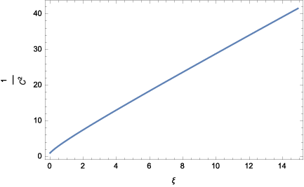
Figure 1: 1/𝒞21/{\cal C}^{2} as a function of ξ\xi.

We numerically solved Eq. (77) for different values of ξ\xi to fix 𝒞⁡(ξ){\cal C}(\xi). From Fig. 1 it is found that

𝒞2≃11+s​ξ,\displaystyle{\cal C}^{2}\simeq\frac{1}{1+s\xi}, (80)

where ss is nearly constant even for larger ξ\xi than plotted and s≳2.4s\gtrsim 2.4. Thus, the primordial tensor spectrum is evaluated as

𝒫h≃1A+s​β​H2​2​H2π2.\displaystyle{\cal P}_{h}\simeq\frac{1}{A+s\beta H^{2}}\frac{2H^{2}}{\pi^{2}}. (81)

It is worth emphasizing that this result is obtained without assuming any particular form of the function f⁡(R,Rμ​ν2,Cμ​ν​ρ​σ2)f(R,R_{\mu\nu}^{2},C_{\mu\nu\rho\sigma}^{2}).

V Discussion and Conclusions

In this paper, we have extended the work of Ref. [21] to more general theories of gravity on a less symmetric background, and shown that cosmological perturbations in f⁡(R,Rμ​ν2,Rμ​ν​ρ​σ2)f(R,R_{\mu\nu}^{2},R_{\mu\nu\rho\sigma}^{2}) gravity can be stabilized by adding constraints to the theory at the level of the quadratic action. We have found that the stabilized theory has two tensor and one scalar polarizations. This indicates that the propagating degrees of freedom are the same as those in scalar-tensor theories, though it involves safe higher spatial derivatives of the metric fluctuations such as ∂t∂2δ​gμ​ν\partial_{t}\partial^{2}\delta g_{\mu\nu} and ∂2∂2δ​gμ​ν\partial^{2}\partial^{2}\delta g_{\mu\nu}. It would therefore be intriguing if one could identify the corresponding scalar-tensor theory. We expect that the ADM description of scalar-tensor theories in the unitary gauge is the optimal way for this purpose, following and generalizing the recently developed approach toward single-scalar theories beyond Horndeski [14, 15]. Helpful hints for guessing the corresponding scalar-tensor description would be obtained by going beyond the quadratic action or by examining perturbations on more general backgrounds such as Kasner spacetime. We hope to report our developments in this direction soon.

We have focused on the universal structure of the action for the tensor perturbations during inflation, and derived the power spectrum of primordial gravitational waves from the stabilized theory. It would be interesting to evaluate the power spectrum of the curvature perturbation to confront the stabilized theory with observations. We will come back to this issue in a future publication.

Acknowledgements.
This work was supported in part by JSPS Grant-in-Aid for Young Scientists (B) No. 24740161 (T.K.).

Appendix A Coefficients cic_{i} in the quadratic action

The following is the list of the coefficients cic_{i} in the action for the scalar perturbations:

c1\displaystyle c_{1} :⁣=\displaystyle:= −6​f1​a2​ℋ2+36​f11​[4​ℋ4−2​ℋ​ℋ′′+(ℋ′)2+ℋ2​ℋ′]+24​f2​[3​ℋ4−2​ℋ​ℋ′′+(ℋ′)2]\displaystyle-6f_{1}a^{2}\mathcal{H}^{2}+36f_{11}\left[4\mathcal{H}^{4}-2\mathcal{H}\mathcal{H}^{\prime\prime}+\left(\mathcal{H}^{\prime}\right)^{2}+\mathcal{H}^{2}\mathcal{H}^{\prime}\right]+24f_{2}\left[3\mathcal{H}^{4}-2\mathcal{H}\mathcal{H}^{\prime\prime}+\left(\mathcal{H}^{\prime}\right)^{2}\right]
+72a2​f12​[22​ℋ6+4​(ℋ′)3+19​ℋ4​ℋ′−8​ℋ3​ℋ′′−14​ℋ​ℋ′​ℋ′′+11​ℋ2​(ℋ′)2]\displaystyle+\frac{72}{a^{2}}f_{12}\left[22\mathcal{H}^{6}+4\left(\mathcal{H}^{\prime}\right)^{3}+19\mathcal{H}^{4}\mathcal{H}^{\prime}-8\mathcal{H}^{3}\mathcal{H}^{\prime\prime}-14\mathcal{H}\mathcal{H}^{\prime}\mathcal{H}^{\prime\prime}+11\mathcal{H}^{2}\left(\mathcal{H}^{\prime}\right)^{2}\right]
+216a2​f111​ℋ​(ℋ2+ℋ′)​(2​ℋ3−ℋ′′)\displaystyle+\frac{216}{a^{2}}f_{111}\mathcal{H}\left(\mathcal{H}^{2}+\mathcal{H}^{\prime}\right)\left(2\mathcal{H}^{3}-\mathcal{H}^{\prime\prime}\right)
+288a4f22[12ℋ8+2(ℋ′)4+21ℋ6ℋ′−4ℋ5ℋ′′+11ℋ4(ℋ′)2\displaystyle+\frac{288}{a^{4}}f_{22}\left[12\mathcal{H}^{8}+2\left(\mathcal{H}^{\prime}\right)^{4}+21\mathcal{H}^{6}\mathcal{H}^{\prime}-4\mathcal{H}^{5}\mathcal{H}^{\prime\prime}+11\mathcal{H}^{4}\left(\mathcal{H}^{\prime}\right)^{2}\right.
−10ℋ(ℋ′)2ℋ′′+11ℋ2(ℋ′)3−10ℋ3ℋ′ℋ′′]\displaystyle\qquad\qquad\left.-10\mathcal{H}\left(\mathcal{H}^{\prime}\right)^{2}\mathcal{H}^{\prime\prime}+11\mathcal{H}^{2}\left(\mathcal{H}^{\prime}\right)^{3}-10\mathcal{H}^{3}\mathcal{H}^{\prime}\mathcal{H}^{\prime\prime}\right]
+864a4​f112​ℋ​[5​ℋ7+ℋ​(ℋ′)3+7​ℋ5​ℋ′−2​ℋ4​ℋ′′+5​ℋ3​(ℋ′)2−4​ℋ2​ℋ′​ℋ′′−3​(ℋ′)2​ℋ′′]\displaystyle+\frac{864}{a^{4}}f_{112}\mathcal{H}\left[5\mathcal{H}^{7}+\mathcal{H}\left(\mathcal{H}^{\prime}\right)^{3}+7\mathcal{H}^{5}\mathcal{H}^{\prime}-2\mathcal{H}^{4}\mathcal{H}^{\prime\prime}+5\mathcal{H}^{3}\left(\mathcal{H}^{\prime}\right)^{2}-4\mathcal{H}^{2}\mathcal{H}^{\prime}\mathcal{H}^{\prime\prime}-3\left(\mathcal{H}^{\prime}\right)^{2}\mathcal{H}^{\prime\prime}\right]
+864a6f122ℋ[16ℋ9+8ℋ(ℋ′)4+32ℋ7ℋ′−5ℋ6ℋ′′+34ℋ5(ℋ′)2+18ℋ3(ℋ′)3\displaystyle+\frac{864}{a^{6}}f_{122}\mathcal{H}\left[16\mathcal{H}^{9}+8\mathcal{H}\left(\mathcal{H}^{\prime}\right)^{4}+32\mathcal{H}^{7}\mathcal{H}^{\prime}-5\mathcal{H}^{6}\mathcal{H}^{\prime\prime}+34\mathcal{H}^{5}\left(\mathcal{H}^{\prime}\right)^{2}+18\mathcal{H}^{3}\left(\mathcal{H}^{\prime}\right)^{3}\right.
−20ℋ2(ℋ′)2ℋ′′−12(ℋ′)3ℋ′′−17ℋ4ℋ′ℋ′′]\displaystyle\qquad\qquad\quad\left.-20\mathcal{H}^{2}\left(\mathcal{H}^{\prime}\right)^{2}\mathcal{H}^{\prime\prime}-12\left(\mathcal{H}^{\prime}\right)^{3}\mathcal{H}^{\prime\prime}-17\mathcal{H}^{4}\mathcal{H}^{\prime}\mathcal{H}^{\prime\prime}\right]
+3456a8​f222​ℋ​[ℋ6+2​(ℋ′)3+3​ℋ4​ℋ′+3​ℋ2​(ℋ′)2]​[4​ℋ5−ℋ2​ℋ′′+2​ℋ​(ℋ′)2−2​ℋ′​ℋ′′],\displaystyle+\frac{3456}{a^{8}}f_{222}\mathcal{H}\left[\mathcal{H}^{6}+2\left(\mathcal{H}^{\prime}\right)^{3}+3\mathcal{H}^{4}\mathcal{H}^{\prime}+3\mathcal{H}^{2}\left(\mathcal{H}^{\prime}\right)^{2}\right]\left[4\mathcal{H}^{5}-\mathcal{H}^{2}\mathcal{H}^{\prime\prime}+2\mathcal{H}\left(\mathcal{H}^{\prime}\right)^{2}-2\mathcal{H}^{\prime}\mathcal{H}^{\prime\prime}\right],
c2\displaystyle c_{2} :⁣=\displaystyle:= 2​(2​f2+3​f11)​(4​ℋ2+3​ℋ′)+24a2​f12​[10​ℋ4−3​ℋ​ℋ′′+6​(ℋ′)2+11​ℋ2​ℋ′]\displaystyle 2\left(2f_{2}+3f_{11}\right)\left(4\mathcal{H}^{2}+3\mathcal{H}^{\prime}\right)+\frac{24}{a^{2}}f_{12}\left[10\mathcal{H}^{4}-3\mathcal{H}\mathcal{H}^{\prime\prime}+6\left(\mathcal{H}^{\prime}\right)^{2}+11\mathcal{H}^{2}\mathcal{H}^{\prime}\right] (83)
+36a2​f111​ℋ​(2​ℋ3−ℋ′′)\displaystyle+\frac{36}{a^{2}}f_{111}\mathcal{H}\left(2\mathcal{H}^{3}-\mathcal{H}^{\prime\prime}\right)
+24a4​f22​[20​ℋ6+12​(ℋ′)3+35​ℋ4​ℋ′−6​ℋ3​ℋ′′−12​ℋ​ℋ′​ℋ′′+32​ℋ2​(ℋ′)2]\displaystyle+\frac{24}{a^{4}}f_{22}\left[20\mathcal{H}^{6}+12\left(\mathcal{H}^{\prime}\right)^{3}+35\mathcal{H}^{4}\mathcal{H}^{\prime}-6\mathcal{H}^{3}\mathcal{H}^{\prime\prime}-12\mathcal{H}\mathcal{H}^{\prime}\mathcal{H}^{\prime\prime}+32\mathcal{H}^{2}\left(\mathcal{H}^{\prime}\right)^{2}\right]
+72a4​f112​ℋ​[8​ℋ5−3​ℋ2​ℋ′′+2​ℋ​(ℋ′)2+8​ℋ3​ℋ′−6​ℋ′​ℋ′′]\displaystyle+\frac{72}{a^{4}}f_{112}\mathcal{H}\left[8\mathcal{H}^{5}-3\mathcal{H}^{2}\mathcal{H}^{\prime\prime}+2\mathcal{H}\left(\mathcal{H}^{\prime}\right)^{2}+8\mathcal{H}^{3}\mathcal{H}^{\prime}-6\mathcal{H}^{\prime}\mathcal{H}^{\prime\prime}\right]
+144a6​f122​ℋ​(ℋ2+2​ℋ′)​[10​ℋ5−3​ℋ2​ℋ′′+4​ℋ​(ℋ′)2+4​ℋ3​ℋ′−6​ℋ′​ℋ′′]\displaystyle+\frac{144}{a^{6}}f_{122}\mathcal{H}\left(\mathcal{H}^{2}+2\mathcal{H}^{\prime}\right)\left[10\mathcal{H}^{5}-3\mathcal{H}^{2}\mathcal{H}^{\prime\prime}+4\mathcal{H}\left(\mathcal{H}^{\prime}\right)^{2}+4\mathcal{H}^{3}\mathcal{H}^{\prime}-6\mathcal{H}^{\prime}\mathcal{H}^{\prime\prime}\right]
+288a8​f222​ℋ​(ℋ2+2​ℋ′)2​[4​ℋ5−ℋ2​ℋ′′+2​ℋ​(ℋ′)2−2​ℋ′​ℋ′′],\displaystyle+\frac{288}{a^{8}}f_{222}\mathcal{H}\left(\mathcal{H}^{2}+2\mathcal{H}^{\prime}\right)^{2}\left[4\mathcal{H}^{5}-\mathcal{H}^{2}\mathcal{H}^{\prime\prime}+2\mathcal{H}\left(\mathcal{H}^{\prime}\right)^{2}-2\mathcal{H}^{\prime}\mathcal{H}^{\prime\prime}\right]~,
c3\displaystyle c_{3} :⁣=\displaystyle:= −4​f1​a2​ℋ+12​f11​(8​ℋ3−ℋ′′)+8​f2​(6​ℋ3−ℋ′′−2​ℋ​ℋ′)\displaystyle-4f_{1}a^{2}\mathcal{H}+12f_{11}\left(8\mathcal{H}^{3}-\mathcal{H}^{\prime\prime}\right)+8f_{2}\left(6\mathcal{H}^{3}-\mathcal{H}^{\prime\prime}-2\mathcal{H}\mathcal{H}^{\prime}\right) (84)
+48a2​f12​[26​ℋ5−8​ℋ2​ℋ′′+ℋ​(ℋ′)2+11​ℋ3​ℋ′−2​ℋ′​ℋ′′]+216a2​f111​(2​ℋ5−ℋ2​ℋ′′)\displaystyle+\frac{48}{a^{2}}f_{12}\left[26\mathcal{H}^{5}-8\mathcal{H}^{2}\mathcal{H}^{\prime\prime}+\mathcal{H}\left(\mathcal{H}^{\prime}\right)^{2}+11\mathcal{H}^{3}\mathcal{H}^{\prime}-2\mathcal{H}^{\prime}\mathcal{H}^{\prime\prime}\right]+\frac{216}{a^{2}}f_{111}\left(2\mathcal{H}^{5}-\mathcal{H}^{2}\mathcal{H}^{\prime\prime}\right)
+48a4f22[60ℋ7+4ℋ(ℋ′)3+70ℋ5ℋ′−19ℋ4ℋ′′\displaystyle+\frac{48}{a^{4}}f_{22}\left[60\mathcal{H}^{7}+4\mathcal{H}\left(\mathcal{H}^{\prime}\right)^{3}+70\mathcal{H}^{5}\mathcal{H}^{\prime}-19\mathcal{H}^{4}\mathcal{H}^{\prime\prime}\right.
+22ℋ3(ℋ′)2−28ℋ2ℋ′ℋ′′−4(ℋ′)2ℋ′′]\displaystyle\qquad\qquad\left.+22\mathcal{H}^{3}\left(\mathcal{H}^{\prime}\right)^{2}-28\mathcal{H}^{2}\mathcal{H}^{\prime}\mathcal{H}^{\prime\prime}-4\left(\mathcal{H}^{\prime}\right)^{2}\mathcal{H}^{\prime\prime}\right]
+144a4​f112​ℋ2​[28​ℋ5−11​ℋ2​ℋ′′+6​ℋ​(ℋ′)2+20​ℋ3​ℋ′−16​ℋ′​ℋ′′]\displaystyle+\frac{144}{a^{4}}f_{112}\mathcal{H}^{2}\left[28\mathcal{H}^{5}-11\mathcal{H}^{2}\mathcal{H}^{\prime\prime}+6\mathcal{H}\left(\mathcal{H}^{\prime}\right)^{2}+20\mathcal{H}^{3}\mathcal{H}^{\prime}-16\mathcal{H}^{\prime}\mathcal{H}^{\prime\prime}\right]
+288a6f122ℋ2[42ℋ7+20ℋ(ℋ′)3+68ℋ5ℋ′−13ℋ4ℋ′′+32ℋ3(ℋ′)2\displaystyle+\frac{288}{a^{6}}f_{122}\mathcal{H}^{2}\left[42\mathcal{H}^{7}+20\mathcal{H}\left(\mathcal{H}^{\prime}\right)^{3}+68\mathcal{H}^{5}\mathcal{H}^{\prime}-13\mathcal{H}^{4}\mathcal{H}^{\prime\prime}+32\mathcal{H}^{3}\left(\mathcal{H}^{\prime}\right)^{2}\right.
−40ℋ2ℋ′ℋ′′−28(ℋ′)2ℋ′′]\displaystyle\qquad\qquad\qquad\left.-40\mathcal{H}^{2}\mathcal{H}^{\prime}\mathcal{H}^{\prime\prime}-28\left(\mathcal{H}^{\prime}\right)^{2}\mathcal{H}^{\prime\prime}\right]
+576a8​f222​ℋ2​[5​ℋ4+8​(ℋ′)2+14​ℋ2​ℋ′]​[4​ℋ5−ℋ2​ℋ′′+2​ℋ​(ℋ′)2−2​ℋ′​ℋ′′],\displaystyle+\frac{576}{a^{8}}f_{222}\mathcal{H}^{2}\left[5\mathcal{H}^{4}+8\left(\mathcal{H}^{\prime}\right)^{2}+14\mathcal{H}^{2}\mathcal{H}^{\prime}\right]\left[4\mathcal{H}^{5}-\mathcal{H}^{2}\mathcal{H}^{\prime\prime}+2\mathcal{H}\left(\mathcal{H}^{\prime}\right)^{2}-2\mathcal{H}^{\prime}\mathcal{H}^{\prime\prime}\right]~,
c4\displaystyle c_{4} :⁣=\displaystyle:= 2​(2​f2+3​f11)​(3​ℋ2−ℋ′)+8a2​f12​[29​ℋ4−8​ℋ​ℋ′′−5​(ℋ′)2+10​ℋ2​ℋ′]\displaystyle 2\left(2f_{2}+3f_{11}\right)\left(3\mathcal{H}^{2}-\mathcal{H}^{\prime}\right)+\frac{8}{a^{2}}f_{12}\left[29\mathcal{H}^{4}-8\mathcal{H}\mathcal{H}^{\prime\prime}-5\left(\mathcal{H}^{\prime}\right)^{2}+10\mathcal{H}^{2}\mathcal{H}^{\prime}\right] (85)
+36a2​f111​ℋ​(2​ℋ3−ℋ′′)\displaystyle+\frac{36}{a^{2}}f_{111}\mathcal{H}\left(2\mathcal{H}^{3}-\mathcal{H}^{\prime\prime}\right)
+8a4​f22​[69​ℋ6−8​(ℋ′)3+71​ℋ4​ℋ′−20​ℋ3​ℋ′′−28​ℋ​ℋ′​ℋ′′+18​ℋ2​(ℋ′)2]\displaystyle+\frac{8}{a^{4}}f_{22}\left[69\mathcal{H}^{6}-8\left(\mathcal{H}^{\prime}\right)^{3}+71\mathcal{H}^{4}\mathcal{H}^{\prime}-20\mathcal{H}^{3}\mathcal{H}^{\prime\prime}-28\mathcal{H}\mathcal{H}^{\prime}\mathcal{H}^{\prime\prime}+18\mathcal{H}^{2}\left(\mathcal{H}^{\prime}\right)^{2}\right]
+24a4​f112​ℋ​[28​ℋ5−11​ℋ2​ℋ′′+6​ℋ​(ℋ′)2+20​ℋ3​ℋ′−16​ℋ′​ℋ′′]\displaystyle+\frac{24}{a^{4}}f_{112}\mathcal{H}\left[28\mathcal{H}^{5}-11\mathcal{H}^{2}\mathcal{H}^{\prime\prime}+6\mathcal{H}\left(\mathcal{H}^{\prime}\right)^{2}+20\mathcal{H}^{3}\mathcal{H}^{\prime}-16\mathcal{H}^{\prime}\mathcal{H}^{\prime\prime}\right]
+48a6f122ℋ[42ℋ7+20ℋ(ℋ′)3+68ℋ5ℋ′−13ℋ4ℋ′′\displaystyle+\frac{48}{a^{6}}f_{122}\mathcal{H}\left[42\mathcal{H}^{7}+20\mathcal{H}\left(\mathcal{H}^{\prime}\right)^{3}+68\mathcal{H}^{5}\mathcal{H}^{\prime}-13\mathcal{H}^{4}\mathcal{H}^{\prime\prime}\right.
+32ℋ3(ℋ′)2−40ℋ2ℋ′ℋ′′−28(ℋ′)2ℋ′′]\displaystyle\qquad\qquad\quad\left.+32\mathcal{H}^{3}\left(\mathcal{H}^{\prime}\right)^{2}-40\mathcal{H}^{2}\mathcal{H}^{\prime}\mathcal{H}^{\prime\prime}-28\left(\mathcal{H}^{\prime}\right)^{2}\mathcal{H}^{\prime\prime}\right]
+96a8​f222​ℋ​[5​ℋ4+8​(ℋ′)2+14​ℋ2​ℋ′]​[4​ℋ5−ℋ2​ℋ′′+2​ℋ​(ℋ′)2−2​ℋ′​ℋ′′].\displaystyle+\frac{96}{a^{8}}f_{222}\mathcal{H}\left[5\mathcal{H}^{4}+8\left(\mathcal{H}^{\prime}\right)^{2}+14\mathcal{H}^{2}\mathcal{H}^{\prime}\right]\left[4\mathcal{H}^{5}-\mathcal{H}^{2}\mathcal{H}^{\prime\prime}+2\mathcal{H}\left(\mathcal{H}^{\prime}\right)^{2}-2\mathcal{H}^{\prime}\mathcal{H}^{\prime\prime}\right].
c5\displaystyle c_{5} :⁣=\displaystyle:= 4​(2​f2+3​f11)​ℋ+16a2​f12​(2​ℋ3+7​ℋℋ′)+16a4​f22​[5​ℋ5+14​ℋ3​ℋ′+8​ℋ​(ℋ′)2].\displaystyle 4\left(2f_{2}+3f_{11}\right){\cal H}+\frac{16}{a^{2}}f_{12}\left(2{\cal H}^{3}+7{\cal H}{\cal H}^{\prime}\right)+\frac{16}{a^{4}}f_{22}\left[5{\cal H}^{5}+14{\cal H}^{3}{\cal H}^{\prime}+8{\cal H}({\cal H}^{\prime})^{2}\right]. (86)

References

  • [1] M. Ostrogradski, Mem. Ac. St. Petersbourg VI 4 (1850) 385.
  • [2] R. P. Woodard, “Avoiding dark energy with 1/r modifications of gravity,” Lect. Notes Phys. 720, 403 (2007) [astro-ph/0601672].
  • [3] R. P. Woodard, “The Theorem of Ostrogradsky,” arXiv:1506.02210 [hep-th].
  • [4] T. j. Chen, M. Fasiello, E. A. Lim and A. J. Tolley, “Higher derivative theories with constraints: Exorcising Ostrogradski’s Ghost,” JCAP 1302, 042 (2013) [arXiv:1209.0583 [hep-th]].
  • [5] A. A. Starobinsky, “A New Type of Isotropic Cosmological Models Without Singularity,” Phys. Lett. B 91, 99 (1980).
  • [6] T. P. Sotiriou and V. Faraoni, “f(R) Theories Of Gravity,” Rev. Mod. Phys. 82, 451 (2010) [arXiv:0805.1726 [gr-qc]].
  • [7] A. De Felice and S. Tsujikawa, “f(R) theories,” Living Rev. Rel. 13, 3 (2010) [arXiv:1002.4928 [gr-qc]].
  • [8] A. Nicolis, R. Rattazzi and E. Trincherini, “The Galileon as a local modification of gravity,” Phys. Rev. D 79, 064036 (2009) [arXiv:0811.2197 [hep-th]].
  • [9] C. Deffayet, G. Esposito-Farese and A. Vikman, “Covariant Galileon,” Phys. Rev. D 79, 084003 (2009) [arXiv:0901.1314 [hep-th]].
  • [10] C. Deffayet, S. Deser and G. Esposito-Farese, “Generalized Galileons: All scalar models whose curved background extensions maintain second-order field equations and stress-tensors,” Phys. Rev. D 80, 064015 (2009) [arXiv:0906.1967 [gr-qc]].
  • [11] G. W. Horndeski, “Second-order scalar-tensor field equations in a four-dimensional space,” Int. J. Theor. Phys. 10, 363 (1974).
  • [12] C. Deffayet, X. Gao, D. A. Steer and G. Zahariade, “From k-essence to generalised Galileons,” Phys. Rev. D 84, 064039 (2011) [arXiv:1103.3260 [hep-th]].
  • [13] T. Kobayashi, M. Yamaguchi and J. Yokoyama, “Generalized G-inflation: Inflation with the most general second-order field equations,” Prog. Theor. Phys. 126, 511 (2011) [arXiv:1105.5723 [hep-th]].
  • [14] J. Gleyzes, D. Langlois, F. Piazza and F. Vernizzi, “Healthy theories beyond Horndeski,” Phys. Rev. Lett. 114, no. 21, 211101 (2015) [arXiv:1404.6495 [hep-th]].
  • [15] X. Gao, “Unifying framework for scalar-tensor theories of gravity,” Phys. Rev. D 90, no. 8, 081501 (2014) [arXiv:1406.0822 [gr-qc]].
  • [16] J. Gleyzes, D. Langlois, F. Piazza and F. Vernizzi, “Exploring gravitational theories beyond Horndeski,” JCAP 1502, 018 (2015) [arXiv:1408.1952 [astro-ph.CO]].
  • [17] C. Lin, S. Mukohyama, R. Namba and R. Saitou, “Hamiltonian structure of scalar-tensor theories beyond Horndeski,” JCAP 1410, no. 10, 071 (2014) [arXiv:1408.0670 [hep-th]].
  • [18] X. Gao, “Hamiltonian analysis of spatially covariant gravity,” Phys. Rev. D 90, no. 10, 104033 (2014) [arXiv:1409.6708 [gr-qc]].
  • [19] C. Deffayet, G. Esposito-Farese and D. A. Steer, “Counting the degrees of freedom of generalized Galileons,” arXiv:1506.01974 [gr-qc].
  • [20] M. Zumalacárregui and J. García-Bellido, “Transforming gravity: from derivative couplings to matter to second-order scalar-tensor theories beyond the Horndeski Lagrangian,” Phys. Rev. D 89, 064046 (2014) [arXiv:1308.4685 [gr-qc]].
  • [21] T. j. Chen and E. A. Lim, “Stabilization of Linear Higher Derivative Gravity with Constraints,” JCAP 1405, 010 (2014) [arXiv:1311.3189 [hep-th]].
  • [22] K. S. Stelle, “Renormalization of Higher Derivative Quantum Gravity,” Phys. Rev. D 16, 953 (1977).
  • [23] A. Hindawi, B. A. Ovrut and D. Waldram, “Consistent spin two coupling and quadratic gravitation,” Phys. Rev. D 53, 5583 (1996) [hep-th/9509142].
  • [24] A. Hindawi, B. A. Ovrut and D. Waldram, “Nontrivial vacua in higher derivative gravitation,” Phys. Rev. D 53, 5597 (1996) [hep-th/9509147].
  • [25] S. M. Carroll, A. De Felice, V. Duvvuri, D. A. Easson, M. Trodden and M. S. Turner, “The Cosmology of generalized modified gravity models,” Phys. Rev. D 71, 063513 (2005) [astro-ph/0410031].
  • [26] A. Nunez and S. Solganik, “Ghost constraints on modified gravity,” Phys. Lett. B 608, 189 (2005) [hep-th/0411102].
  • [27] T. Chiba, “Generalized gravity and ghost,” JCAP 0503, 008 (2005) [gr-qc/0502070].
  • [28] G. Calcagni, S. Tsujikawa and M. Sami, “Dark energy and cosmological solutions in second-order string gravity,” Class. Quant. Grav. 22, 3977 (2005) [hep-th/0505193].
  • [29] I. Navarro and K. Van Acoleyen, “Consistent long distance modification of gravity from inverse powers of the curvature,” JCAP 0603, 008 (2006) [gr-qc/0511045].
  • [30] A. De Felice, M. Hindmarsh and M. Trodden, “Ghosts, Instabilities, and Superluminal Propagation in Modified Gravity Models,” JCAP 0608, 005 (2006) [astro-ph/0604154].
  • [31] A. De Felice and T. Suyama, “Vacuum structure for scalar cosmological perturbations in Modified Gravity Models,” JCAP 0906, 034 (2009) [arXiv:0904.2092 [astro-ph.CO]].
  • [32] A. D. Felice and T. Tanaka “Inevitable ghost and the degrees of freedom in f⁡(R,𝒢)f(R,\mathcal{G}) gravity,” Prog. Theor. Phys. 124 (3) (2010) [arXiv:1006.4399v2[astro-ph.CO]]
  • [33] M. Lagos, M. Bañados, P. G. Ferreira and S. García-Sáenz, “Noether Identities and Gauge-Fixing the Action for Cosmological Perturbations,” Phys. Rev. D 89, 024034 (2014) [arXiv:1311.3828 [gr-qc]].
  • [34] P. Horava, “Quantum Gravity at a Lifshitz Point,” Phys. Rev. D 79, 084008 (2009) [arXiv:0901.3775 [hep-th]].