Flip the Cloud: Cyber-physical Signaling Games in the Presence of Advanced Persistent Threats
Abstract
Access to the cloud has the potential to provide scalable and cost effective enhancements of physical devices through the use of advanced computational processes run on apparently limitless cyber infrastructure. On the other hand, cyber-physical systems and cloud-controlled devices are subject to numerous design challenges; among them is that of security. In particular, recent advances in adversary technology pose Advanced Persistent Threats (APTs) which may stealthily and completely compromise a cyber system. In this paper, we design a framework for the security of cloud-based systems that specifies when a device should trust commands from the cloud which may be compromised. This interaction can be considered as a game between three players: a cloud defender/administrator, an attacker, and a device. We use traditional signaling games to model the interaction between the cloud and the device, and we use the recently proposed FlipIt game to model the struggle between the defender and attacker for control of the cloud. Because attacks upon the cloud can occur without knowledge of the defender, we assume that strategies in both games are picked according to prior commitment. This framework requires a new equilibrium concept, which we call Gestalt Equilibrium, a fixed-point that expresses the interdependence of the signaling and FlipIt games. We present the solution to this fixed-point problem under certain parameter cases, and illustrate an example application of cloud control of an unmanned vehicle. Our results contribute to the growing understanding of cloud-controlled systems.
1 Introduction
Advances in computation and information analysis have expanded the capabilities of the physical plants and devices in cyber-physical systems (CPS)[4, 13]. Fostered by advances in cloud computing, CPS have garnered significant attention from both industry and academia. Access to the cloud gives administrators the opportunity to build virtual machines that provide to computational resources with precision, scalability, and accessibility.
Despite the advantages that cloud computing provides, it also has some drawbacks. They include - but are not limited to - accountability, virtualization, and security and privacy concerns. In this paper, we focus especially on providing accurate signals to a cloud-connected device and deciding whether to accept those signals in the face of security challenges.
Recently, system designers face security challenges in the form of Advanced Persistent Threats (APTs) [19]. APTs arise from sophisticated attackers who can infer a user’s cryptographic key or leverage zero-day vulnerabilities in order to completely compromise a system without detection by the system administrator [16]. This type of stealthy and complete compromise has demanded new types of models [6, 20] for prediction and design.
In this paper, we propose a model in which a device decides whether to trust commands from a cloud which is vulnerable to APTs and may fall under adversarial control. We synthesize a mathematical framework that enables devices controlled by the cloud to intelligently decide whether to obey commands from the possibly-compromised cloud or to rely on their own lower-level control.
We model the cyber layer of the cloud-based system using the recently proposed FlipIt game [6, 20]. This game is especially suited for studying systems under APTs. We model the interaction between the cloud and the connected device using a signaling game, which provides a framework for modeling dynamic interactions in which one player operates based on a belief about the private information of the other. A significant body of research has utilized this framework for security [7, 9, 15, 21, 8]. The signaling and FlipIt games are coupled, because the outcome of the FlipIt game determines the likelihood of benign and malicious attackers in the robotic signaling game. Because the attacker is able to compromise the cloud without detection by the defender, we consider the strategies of the attacker and defender to be chosen with prior commitment. The circular dependence in our game requires a new equilibrium concept which we call a Gestalt equilibrium11 1 Gestalt is a noun which means something that is composed of multiple parts and yet is different from the combination of the parts [2].. We specify the parameter cases under which the Gestalt equilibrium varies, and solve a case study of the game to give an idea of how the Gestalt equilibrium can be found in general. Our proposed framework has versatile applications to different cloud-connected systems such as urban traffic control, drone delivery, design of smart homes, etc. We study one particular application in this paper:ef control of an unmanned vehicle under the threat of a compromised cloud.
Our contributions are summarized as follows:
- i)
-
We model the interaction of the attacker, defender/cloud administrator, and cloud-connected device by introducing a novel game consisting of two coupled games: a traditional signaling game and the recently proposed FlipIt game.
- ii)
-
We provide a general framework by which a device connected to a cloud can decide whether to follow its own limited control ability or to trust the signal of a possibly-malicious cloud.
- iii)
-
We propose a new equilibrium definition for this combined game: Gestalt equilibrium, which involves a fixed-point in the mappings between the two component games.
- iv)
-
Finally, we apply our framework to the problem of unmanned vehicle control.
In the sections that follow, we first outline the system model, then describe the equilibrium concept. Next, we use this concept to find the equilibria of the game under selected parameter regimes. Finally, we apply our results to the control of an unmanned vehicle. In each of these sections, we first consider the signaling game, then consider the FlipIt game, and last discuss the synthesis of the two games. Finally, we conclude the paper and suggest areas for future research.
2 System Model
We model a cloud-based system in which a cloud is subject to APTs. In this model, an attacker, denoted by , capable of APTs can pay an attack cost to completely compromise the cloud without knowledge of the cloud defender. The defender, or cloud administrator, denoted by , does not observe these attacks, but has the capability to pay a cost to reclaim control of the cloud. The cloud transmits a message to a robot or other device, denoted by . The device may follow this command, but it is also equipped with an on-board control system for autonomous operation. It may elect to use its autonomous operation system rather than obey commands from the cloud.
This scenario involves two games: the FlipIt game introduced in [20], and the well-known signaling game. The FlipIt game takes place between the attacker and cloud defender, while the signaling game takes place between the possibly-compromized cloud and the device. For brevity, denote the FlipIt game by , the signaling game by , and the combined game - call it CloudControl - by as shown in Fig. 1. In the next subsections, we formalize this game model.
2.1 Cloud-Device Signaling Game
Let denote the type of the cloud. Denote compromized and safe types of clouds by and in the set . Denote the probabilities that and that by and . Signaling games typically give these probabilities apriori, but in CloudControl they are determined by the equilibrium of the FlipIt game .
Let and denote messages of high and low risk, respectively, and let represent a message in general. After receives the message, it chooses an action, , where represents trusting the cloud and represents not trusting the cloud.
For the device , let , where . is a utility function such that gives the device’s utility when the type is , the message is , and the action is . Let and be utility functions for the attacker and defender. Note that these players only receive utility in if their own type controls the cloud in , so that type is not longer a necessary argument for and .
Denote the strategy of by , such that gives the mixed-strategy probability that plays action when the message is . The role of the sender may be played by or depending on the state of the cloud, determined by . Let denote the strategy that plays when she controls the cloud, so that gives the probability that sends message . (The superscript specifies that this strategy concerns the signaling game.) Similarly, let denote the strategy played by when he controls the cloud. Then gives the probability that sends message . Let , , and denote the sets of mixed strategies for each player.
For , define functions , such that gives the expected utility to sender when he or she plays mixed-strategy and the receiver plays mixed-strategy . Equation (1) gives .
| (1) |
Next, let represent the belief of , such that gives the likelihood with which believes that a sender who issues message is of type . Then define such that gives the expected utility for when it has belief , the message is , and it plays strategy . is given by
| (2) |
The expected utilities to the sender and receiver will determine their incentives to control the cloud in the game described in the next subsection.
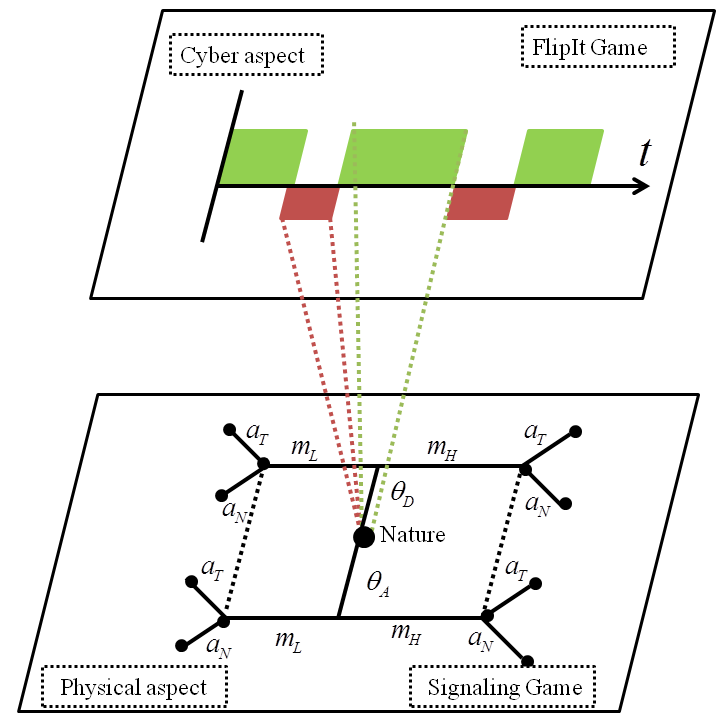
2.2 FlipIt Game for Cloud Control
The basic version of FlipIt [20]22 2 See [20] for a more comprehensive definition of the players, time, game state, and moves in FlipIt. Here, we move on to describing aspects of our game important for analyzing . is played in continuous time. Assume that the defender controls the resource - here, the cloud - at . Moves for both players obtain control of the cloud if it is under the other player’s control. In this paper, we limit our analysis to periodic strategies, in which the moves of the attacker and the moves of the defender are both spaced equally apart, and their phases are chosen randomly from a uniform distribution. Let and (where represents non-negative real numbers) denote the attack and renewal frequencies, respectively.
Players benefit from controlling the cloud, and incur costs from moving. Let denote the average proportion of the time that player has controlled the cloud up to time . Denote the number of moves up to per unit time of player by . Let and represent the costs of each defender and attacker move. In the original formulation of FlipIt, the authors consider a fixed benefit for controlling the cloud. In our formulation, the benefit depends on the equilibrium outcomes of the signaling game . Denote these equilibrium utilities of and by and . These give the expected benefit of controlling the cloud. Finally, let and denote the time-averaged benefit of and up to time in . Then
| (3) |
and, as time continues to evolve, the average benefits over all time become
| (4) |
We next express these expected utilities over all time as a function of periodic strategies that and employ. Let , be expected utility functions such that and give the average utility to and , respectively, when they play with frequencies and . If , it can be shown that
| (5) |
| (6) |
while if , then
| (7) |
| (8) |
and if , we have
| (9) |
3 Solution Concept
In this section, we develop a new equilibrium concept for our CloudControl game . We study the equilibria of the FlipIt and signaling games individually, and then show how they can be related through a fixed-point equation in order to obtain an overall equilibrium for
3.1 Signaling Game Equilibrium
Signaling games are a class of dynamic Bayesian games. Applying the concept of perfect Bayesian equilibrium (as it e.g., [10]) to , we have Definition 1.
Definition 1
Next, let , , and be the utilities for the defender, attacker, and device, respectively, when they play according to a strategy profile and belief that satisfy the conditions for a perfect Bayesian equilibrium. Define a set-valued mapping such that gives the set of equilibrium utilities of the defender and attacker when the prior probabilities are and and the signaling game utilities are parameterized by 33 3 Since does not take part in , it is not necessary to include as an output of the mapping. . We have
| (14) |
We will employ as part of the definition of an overall equilibrium for after examining the equilibrium of the FlipIt game.
3.2 FlipIt Game Equilibrium
The appropriate equilibrium concept for the FlipIt game, when and are restricted to periodic strategies, is Nash equilibrium [14]. Definition 2 applies the concept of Nash Equilibrim to .
Definition 2
To find an overall equilibrium of , we are interested in the proportion of time that and control the cloud. As before, denote these proportions by and , respectively. These proportions (as in [6]) can be found from the equilibrium frequencies by
| (17) |
Let parameterize the FlipIt game. Now, we can define a mapping such that the expression gives the proportion of time that the attacker controls the cloud in equilibrium from the values of controlling the cloud for the defender and the attacker. This mapping gives
| (18) |
In addition to interpreting as the proportion of time that the attacker controls the cloud, we can view it as the likelihood that, at any random time, the cloud will be controlled by the attacker. Of course, this is precisely the value of interest in . Clearly, and are coupled by Equations (14) and (18). These two equations specify the overall equilibrium for the CloudControl game through a fixed-point equation, which we describe next.
3.3 Gestalt Equilibrium of
When the CloudControl game is in equilibrium the mapping from the parameters of to that game’s equilibrium and the mapping from the parameters of to that game’s equilibrium are simultaneously satisfied as shown in Fig. 2. Definition 3 formalizes this equilibrium, which we call Gestalt equilibrium.
Definition 3
(Gestalt equilibrium) The cloud control ratio and equilibrium signaling game utilities and constitute a Gestalt equilibrium of the game composed of coupled games and if the two components of Equation (19) are simultaneously satisfied.
| (19) |
In short, the signaling game utilities must satisfy the fixed-point equation
| (20) |
Solving for the equilibrium of requires a fixed-point equation essentially because the games and are played according to prior committment. Prior commitment specifies that players in do not know the outcome of . This structure prohibits us from using a sequential concept such as sub-game perfection and suggests instead a fixed-point equation.
4 Analysis
In this section, we analyze the game proposed in Section 2 based on our solution concept in Section 3. First, we analyze the signaling game and calculate the corresponding equilibria. Then, we solve the game for different values of expected payoffs resulting from signaling game. Finally, we describe the solution of the combined game.
4.1 Signaling Game Analysis
The premise of allows us to make some basic assumptions about the utility parameters that simplifies the search for equilibria. We expect these assumptions to be true across many different contexts.
- A1)
-
: It is beneficial for the receiver to trust a low risk message from the defender.
- A2)
-
: It is harmful for the receiver to trust a high risk message from the attacker.
- A3)
-
and : Both types of sender prefer that either of their messages is trusted rather than that either of their messages is rejected.
- A4)
-
: The attacker prefers an outcome in which the receiver trusts his high risk message to an outcome in which the receiver trusts his low risk message.
Pooling equilibria of the signaling game differ depending on the prior probabilities and . Specifically, the messages on which and pool and the equilibrium action of depend on quantities in Equations (21) and (22) which we call trust benefits.
| (21) |
| (22) |
and give the benefit of trusting (compared to not trusting) high and low messages, respectively, when the prior probability is . These quantities specify whether will trust a message that it receives in a pooling equilibrium. If (respectively, ) is positive, then, in equilibrium, will trust all messages when the senders pool on (respectively, ).
We illustrate the different possible combinations of and in the quadrants of Fig. 3. The labeled messages and actions for the sender and receiver, respectively, in each quadrant denote these pooling equilibria. These pooling equilibria apply throughout each entire quadrant. Note that we have not listed the requirements on belief here. These are addressed in the Appendix 0.A.2, and become especially important for various equilibrium refinement procedures.
The shaded regions of Fig. 3 denote additional special equilibria which only occur under the additional parameter constraints listed within the regions. (The geometrical shapes of the shaded regions are not meaningful, but their overlap and location relative to the four quadrants are accurate.) The dotted and uniformly shaded zones contain equilibria similar to those already denoted in the equilibria for each quadrant, except that they do not require restrictions on . The zone with horizontal bars denotes the game’s only separating equilibrium. It is a rather unproductive one for and , since their messages are not trusted. (See the derivation in Appendix 0.A.1.) The equilibria depicted in Fig. 3 will become the basis of analyzing the mapping , which will be crucial for forming our fixed-point equation that defines the Gestalt equilibrium. Before studying this mapping, however, we first analyze the equilibria of the FlipIt game on its own.
4.2 FlipIt Analysis
In this subsection, we calculate the Nash equilibrium in the FlipIt game. Equations (5)-(9) represent both players’ utilities in FlipIt game. The solution of this game is similar to what has presented in [20, 6], except that the reward of controlling the resource may vary. To calculate Nash equilibrium, we normalize both players’ benefit with respect to the reward of controlling the resource. For different cases, the frequencies of move at Nash equilibrium are:
and :
| (23) |
and :
| (24) |
and :
| (25) |
:
| (26) |
and :
| (27) |
In the case that , the attacker has no incentive to attack the cloud. In this case, the defender need not move since we assume that she controls the cloud initially. In the case that and , only the attacker has an incentive to control the cloud. We use to signify that the attacker moves only once. Since the defender never moves, the attacker’s single move is enough to retain control of the cloud at all times.
Next, we put together the analysis of and in order to study the Gestalt equilibria of the entire game.
4.3 Analysis
To identify the Gestalt Equilibrium of , it is necessary to examine the mapping for all . As noted in Section 4.1, this mapping depends on and . From assumptions A1-A4, it is possible to verify that must fall in Quadrant I or Quadrant IV and that must lie in Quadrant III or Quadrant IV. There are numerous ways in which the set can transverse different parameter regions. Rather than enumerating all of them, we consider one here.
Consider parameters such that and but 44 4 These parameters must satisfy and . Here, we give them specific values in order to plot the data.. This leads to an that will traverse from Quadrant I to Quadrant IV. Let us also assume that , so that Equilibrium 5 is not feasible. In Fig. 4, we give specific values of parameters that satisfy these conditions, and we plot for . Then, in Table 1, we give the equilibria in each region that the line segment traverses. The equilibrium numbers refer to the derivations in the Appendix 0.A.2.
| Region | Equilibria |
|---|---|
| Quadrant I | |
| Axis | |
| Quadrant IV |
If is such that the signaling game is played in Quadrant I, then both senders prefer pooling on . By the first mover advantage, they will select Equilibrium 8. On the border between Quadrant I and Quadrant IV, and both prefer an equilibrium in which plays . If they pool on , this is guaranteed. If they pool on , however, receives equal utility for playing and ; thus, the senders cannot guarantee that the receiver will play . Here, we assume that the senders maximize their worst-case utility, and thus pool on . This is Equilibrium 3. Finally, in Quadrant IV, both senders prefer to be trusted, and so select Equilibrium 3. From the table, we can see that the utilities will have a jump at the border between Quadrant I and Quadrant IV. The solid line in Fig. 5 plots the ratio of the utilities as a function of .
Next, consider the mapping . As we have noted, depends only on the ratio 55 5 When , we define that ratio to be equal to zero, since this will yield and , as in Equations (9) and (17). When and , it is convenient to consider the ratio to be positively infinite since this is consistent with . . Indeed, it is continuous in that ratio when the outcome at the endpoints is appropriately defined. This mapping is represented by the dashed line in Fig. 5, with the independent variable on the vertical axis.
We seek a fixed-point, in which and . This shown by the intersection of the solid and dashed curves plotted in Fig. 5. At these points, the mappings between the signaling and the FlipIt games are mutually satisfied, and we have a Gestalt equilibrium.66 6 Note that this example featured a discontinuity in signaling game utilities on the border between equilibrium regions. Interestingly, even when the pooling equilibria differ between regions, it is possible that the equilibrium on the border admits a mixed strategy that provides continuity between the different equilibria in the two regions, and thus makes continuous. This could allow to have multiple Gestalt equilibria.
5 Cloud Control Application
In this section, we describe one possible application of our model: a cyber-physical system composed of autonomous vehicles with some on-board control but also with the ability to trust commands from the cloud. Access to the cloud can offer automated vehicles several benefits [12]. First, it allows access to massive computational resources - i.e., infrastructure as a service (IaaS). (See [5].) Second, it allows access to large datasets. These datasets can offer super-additive benefits to the sensing capabilities of the vehicle itself, as in the case of the detailed road and terrain maps that automated cars such as those created by Google and Delphi combine with data collected by lidar, radar and vision-based cameras [1, 11]. Third, interfacing with the cloud allows access to data collected or processed by humans through crowd-sourcing applications; consider, for instance, location-based services [17, 18] that feature recommendations from other users. Finally, the cloud can allow vehicles to collectively learn through experience [12].
Attackers may attempt to influence cloud control of the vehicle through several means. In one type of attack, adversaries may be able to steal or infer cryptographic keys that allow them authorization into the network. These attacks are of the complete compromise and stealth types that are studied in the FlipIt framework [20], [6] and thus are appropriate for a CloudControl game. FlipIt also provides the ability to model zero-day exploits, vulnerabilities for which a patch is not currently available. Each of these types of attacks on the cloud pose threats to unmanned vehicle security and involve the complete compromise and steathiness that motivate the FlipIt framework.
5.1 Dynamic Model for Cloud Controlled Unmanned Vehicles
In this subsection, we use a dynamic model of an autonomous car to illustrate one specific context in which a cloud-connected device could be making a decision of whether to trust the commands that it would receive or to follow its own on-board control.
We consider a car moving in two-dimensional space with a fixed speed but with steering that can be controlled. (See Fig. 6, which illustrates the “bicycle model” of steering control from [3].) For simplicity, assume that we are interested in the car’s deviation from a straight line. (This line might, e.g., run along the center of the proper driving lane.) Let denote the car’s vertical distance from the horizontal line, and let denote the heading of the car at time . The state of the car can be represented by a two-dimensional vector . Let denote the angle between the orientation of the front wheel - which implements steering - and the orientation of the length of the car. We can consider to be the input to the system. Finally, let represent a vector of outputs available to the car’s control system. The self-driving cars of both Google and Delphi employ radar, lidar, and vision-based cameras for localization. Assume that these allow accurate measurement of both states, such that and . If the car stays near , then we can approximate the system with a linear model. Let and denote the distances from the rear wheel to the center of gravity and the rear wheel to the front wheel of the car, respectively. Then the linearized system is given in [3] by the equations:
| (28) |
| (29) |
5.2 Control of Unmanned Vehicle
Assume that the unmanned car has some capacity for automatic control without the help of the cloud, but that the cloud typically provides more advanced navigation.
Specifically, consider a control system onboard the unmanned vehicle designed to return it to the equilibrium . Because the car has access to both of the states, it can implement a state-feedback control. Consider a linear, time-invariant control of the form
| (30) |
This proportional control results in the closed-loop system
| (31) |
The unmanned car may also elect to obtain data or computational resources from the cloud. Typically, this additional access would improve the control of the car. The cloud administrator (defender ), however, may issue faulty commands or there may be a breakdown in communication of the desired signals. In addition, the cloud may be compromised by in a way that is stealthy. Because of these factors, sometimes benefits from rejecting the cloud’s command and relying on its own navigational abilities. Denote the command issued by the cloud at time by , depending on who controls the cloud. With this command, the system is given by
| (32) |
5.3 Filter for High Risk Cloud Commands
In cloud control of an unmanned vehicle, the self-navigation state feedback input given by in Equation (30) represents the control that is expected by the vehicle given its state. If the signal from the cloud differs significantly from the signal given by the self-navigation system, then the vehicle may classify the message as “high-risk.” Specifically, define a difference threshold , and let
| (33) |
Equation (33) translates the actual command from the cloud (controlled by or ) into a message in the cloud signaling game.
Equations (31) and (32) give the dynamics of the unmanned car electing to trust and not trust the cloud. Based on these equations, Fig. 7 illustrates the combined self-navigating and cloud controlled system for vehicle control.

6 Conclusion and Future Work
In this paper, we have proposed a general framework for the interaction between an attacker, cloud administrator/defender, and cloud-connected device. We have described the struggle for control of the cloud using the FlipIt game and the interaction between the cloud and the connected device using a traditional signaling game. Because these two games are played by prior commitment, they are coupled. We have defined a new equilibrium concept - i.e., Gestalt equilibrium, which defines a solution to the combined game using a fixed-point equation. After illustrating various parameter regions under which the game may be played, we solved the game in a sample parameter region. Finally, we showed how the framework may be applied to unmanned vehicle control.
Several directions remain open for future work. First, the physical component of the cyber-physical system can be further examined. Tools from optimal control such as the linear-quadratic regulator could offer a rigerous framework for defining the costs associated with the physical dynamic system, which in turn would define the payoffs of the signaling game. Second, future work could search for conditions under which a Gestalt equilibrium of the CloudControl game is guaranteed to exist. Finally, devices that use this framework should be equipped to learn online. Towards that end, a learning algorithm could be developed that is guaranteed to converge to the Gestalt equilibrium. Together with the framework developed in the present paper, these directions would help to advance our ability to secure cloud-connected and cyber-physical systems.
References
- [1] Delphi drive, Delphi Automotive, [Online]. Available: http://www.delphi.com/delphi-drive.
- [2] Gestalt, Mirium-Webster, [Online]. Available: http://www.merriam-webster.com/dictionary/gestalt.
- [3] K.l J. Aström and R. M. Murray, Feedback systems: an introduction for scientists and engineers, Princeton university press, 2010.
- [4] R. Baheti and H. Gill, Cyber-physical systems, The impact of control technology 12 (2011), 161–166.
- [5] S. Bhardwaj, L. Jain, and S. Jain, Cloud computing: A study of infrastructure as a service (iaas), International Journal of engineering and information Technology 2 (2010), no. 1, 60–63.
- [6] K. D. Bowers, M. Van Dijk, R. Griffin, A. Juels, A. Oprea, R. L. Rivest, and N. Triandopoulos, Defending against the unknown enemy: Applying flipit to system security, Decision and Game Theory for Security, Springer, 2012, pp. 248–263.
- [7] Thomas E Carroll and Daniel Grosu, A game theoretic investigation of deception in network security, Security and Communication Networks 4 (2011), no. 10, 1162–1172.
- [8] William Casey, Jose A. Morales, Thomson Nguyen, Jonathan Spring, Rhiannon Weaver, Evan Wright, Leigh Metcalf, and Bud Mishra, Cyber security via signaling games: Toward a science of cyber security, Distributed Computing and Internet Technology (Raja Natarajan, ed.), Lecture Notes in Computer Science, vol. 8337, Springer International Publishing, 2014, pp. 34–42 (English).
- [9] S. Farhang, M. H. Manshaei, M. N. Esfahani, and Q. Zhu, A dynamic bayesian security game framework for strategic defense mechanism design, Decision and Game Theory for Security, Springer, 2014, pp. 319–328.
- [10] D. Fudenberg and J. Tirole, Game theory. 1991, Cambridge, Massachusetts 393 (1991).
- [11] E. Guizzo, How google’s self-driving car works, IEEE Spectrum Online, October 18 (2011).
- [12] B. Kehoe, S. Patil, P. Abbeel, and K. Goldberg, A survey of research on cloud robotics and automation, Automation Science and Engineering, IEEE Transactions on 12 (2015), no. 2, 398–409.
- [13] E. A. Lee, Cyber physical systems: Design challenges, Object Oriented Real-Time Distributed Computing (ISORC), 2008 11th IEEE International Symposium on, IEEE, 2008, pp. 363–369.
- [14] John F Nash et al., Equilibrium points in n-person games, Proc. Nat. Acad. Sci. USA 36 (1950), no. 1, 48–49.
- [15] J. Pawlick and Q. Zhu, Deception by design: Evidence-based signaling games for network defense, arXiv preprint arXiv:1503.05458 (2015).
- [16] G. Portokalidis, A. Slowinska, and H. Bos, Argos: an emulator for fingerprinting zero-day attacks for advertised honeypots with automatic signature generation, ACM SIGOPS Operating Systems Review, vol. 40, ACM, 2006, pp. 15–27.
- [17] K. Sampigethaya, L. Huang, M. Li, R. Poovendran, K. Matsuura, and K. Sezaki, Caravan: Providing location privacy for vanet, Tech. report, DTIC Document, 2005.
- [18] K. Sampigethaya, M. Li, L. Huang, and R. Poovendran, Amoeba: Robust location privacy scheme for vanet, Selected Areas in Communications, IEEE Journal on 25 (2007), no. 8, 1569–1589.
- [19] C. Tankard, Advanced persistent threats and how to monitor and deter them, Network security 2011 (2011), no. 8, 16–19.
- [20] M. van Dijk, A. Juels, A. Oprea, and R. L. Rivest, Flipit: The game of “stealthy takeover”, Journal of Cryptology 26 (2013), no. 4, 655–713.
- [21] J. Zhuang, V. M. Bier, and O. Alagoz, Modeling secrecy and deception in a multiple-period attacker–defender signaling game, European Journal of Operational Research 203 (2010), no. 2, 409–418.
Appendix 0.A Derivation of Signaling Game Equilibria
In this appendix, we solve for the equilibria of .
0.A.1 Separating Equilibria
First, we search for separating equilibria of . In separating equilibria, knows with certainty the type of the cloud.
plays and plays
If plays (as a pure strategy) and plays , then the receiver rejects any according to assumption A2. The best action for is to deviate to . Thus, this is not an equilibrium.
plays and plays
If plays and plays , the ’s best response depends on the utility parameters. If and , then plays in response to both messages. There is no incentive to deviate. Denote this separating equilibrium as Equilibrium #2.
If and , then is within the set of best responses to , whereas is the unique best response to . Assuming that he prefers to certainty receive a higher utility, deviates to .
If and , then is within the set of best responses to , whereas is the unique best response to . Thus, deviates to .
If and , then plays in response to both messages. We have assumed, however, that prefers to be trusted on compared to being trusted on (A4), so deviates and this is not an equilibrium.
0.A.2 Pooling Equilibria
Next, we search for pooling equilibria of . In pooling equilibria, relies only on the prior probabilities and in order to form his belief about the type of the cloud. The existence of pooling equilibria depend essentially on the trust benefits and
Pooling on
If , then ’s best response is . This will only be an equilibrium if his best response to would also be . This is the case only when the belief satisfies
| (34) |
Moreover, this can only be an equilibrium when neither nor have an incentive to deviate: i.e., when
| (35) |
If these conditions are satisfied, then denote this equilibrium by Equilibrium #1.
If , then ’s best response us . Whether this represents an equilibrium depends on if or have incentives to deviate from . If and , then neither has an incentive to deviate. This is Equilibrium #5. If one of these inequalities does not hold, then the player who prefers to will deviate if would play in response to the deviation. The equilibrium condition is narrowed to when the belief makes not trust ; when Equation (34) is satisfied. Call this Equilibrium #3.
Pooling on
The pattern of equilibria for pooling on follows a similar structure to the pattern of equilibria for pooling on .
If , then ’s best response is . This will only be an equilibrium if his best response to would also be . This is the case only when the belief satisfies
| (36) |
To guarantee that and do not deviate, we require
| (37) |
If these conditions are satisfied, then we have Equilibrium #6.
If , then ’s best response is . If and , then neither nor have an incentive to deviate. Call this Equilibrium #8. If one of these inequalities does not hold, then the belief must satisfy Equation (36) for an equilibrium to be sustained. Denote this equilibrium by Equilibrium #7.