Computing the Size of Intervals in the Weak Bruhat Order

A permutation of $n$ is a bijective function from $[n]=\{1,2,\ldots,n\}$ onto itself; we write ${\mathcal{S}}_{n}$ for the set of all permutations of $n$. We denote the composition of two permutations, $f$ and $g$, by $fg$, i.e., $fg(x)=f(g(x))$. A permutation $\sigma$ is sometimes identified with the string $\sigma(1)\sigma(2)\ldots\sigma(n)$, its expression in so-called one-line notation. The width of a permutation $\sigma$ is the length of its longest decreasing subsequence, denoted $\width(\sigma)$. A transposition reversing $k$ and $l$ in $[n]$ is a permutation $\sigma$ with $\sigma(k)=l$, $\sigma(l)=k$, and $\sigma(i)=i$ for $i\not\in\{l,k\}$. If $|k-l|=1$, then we say that $\sigma$ is an adjacent transposition.

A poset of size $n$ is a pair $P=(S,\prec)$ where $S$ is a set of cardinality $n$, and $\prec$ is a partial order relation, that is, a binary relation which is reflexive, transitive, and antisymmetric. If $p\prec q$ or $q\prec p$, then we say that $p$ and $q$ are comparable, and incomparable otherwise. Given a poset $P=(S,\prec)$, a linear extension of $P$ is a total order $\prec^{\prime}$ on $S$ such that, for all $p,q\in S$, $p\prec q$ implies $p\prec^{\prime}q$. Equivalently, $\prec^{\prime}$ is a total order with $\prec\subseteq\prec^{\prime}$ as relations. The set of all linear extensions of $P$ is denoted ${\mathcal{L}}(P)$. An interval $[p,q]$ of a poset $P=(S,\prec)$ is the set $\{r\in S|p\prec r\prec q\}$. A chain $C\subseteq S$ is a subset of pairwise comparable elements, and an antichain $A\subseteq S$ is a set of pairwise incomparable elements. The width of a poset $P$ is the cardinality of its largest antichain.

Given a poset $P=(S,\prec)$, a collection of linear extensions ${\mathcal{R}}=\{\prec_{1},\prec_{2},\ldots,\prec_{k}\}$ is called a realizer of $P$ if $\prec=\bigcap_{i=1}^{k}\prec_{k}$, where each relation $\prec_{i}$ is interpreted as a set of ordered pairs. Equivalently, ${\mathcal{R}}$ is a realizer of $P$ if, for all $p,q\in S$, $p\prec q$ if and only if $p\prec_{i}q$ for all $1\leq i\leq k$. A realizer is said to be minimal if it has the smallest possible cardinality among all realizers of $P$. The dimension of $P$ is the cardinality of any minimal realizer.

We now define the weak Bruhat order on permutations of $n$, an important structure in algebraic combinatorics and elsewhere. Given two permutations $\sigma_{1}$ and $\sigma_{2}$, we have the covering relation $\sigma_{1}\lessdot\sigma_{2}$ if and only if there is an adjacent transposition $\tau$ reversing $k$ and $l$ with $\sigma_{1}=\sigma_{2}\tau$, $k<l$, and $\sigma_{1}(k)<\sigma_{1}(l)$. The reflexive and transitive closure of $\lessdot$ gives the partial ordering relation for the weak Bruhat order. The weak Bruhat order on ${\mathcal{S}}_{3}$ is depicted in Figure 1.

The present work investigates computational complexity questions regarding the structures we have just defined. We refer to standard texts in computational complexity theory to precisely define hardness of decision and functional complexity problems (e.g., [2]). Roughly, a decision problem is in ${\bf P}$ if the answer can be computed in polynomial time (in the size of the input instance); it is in ${\bf NP}$ if the answer can be certified in polynomial time; it is ${\bf NP}$-hard if every problem in ${\bf NP}$ can be reduced to it in polynomial time (i.e., it is at least as hard as all problems in ${\bf NP}$). Similarly, a function problem (a computational problem whose output is an integer instead of only a single bit) is in ${\bf FP}$ if the answer can be computed in polynomial time (in the size of the input instance); it is in $\#{\bf P}$ if it consists of computing the number of correct solutions to a problem in ${\bf NP}$; it is $\#{\bf P}$-hard if the problem of computing the number of correct solutions to any problem in ${\bf NP}$ can be reduced to this problem in polynomial time.

These two ideas, the weak Bruhat order on ${\mathcal{S}}_{n}$ and poset linear extensions, give rise to many computational complexity questions. We address two in particular. First, how hard is it to compute interval sizes in the weak Bruhat order? In particular, given permutations $\sigma_{1}$ and $\sigma_{2}$ of $n$, what is the computational complexity of computing the size of the interval $[\sigma_{1},\sigma_{2}]$ in the weak Bruhat order on ${\mathcal{S}}_{n}$? Wei gives an explicit formula for the case when $\sigma_{2}\sigma_{1}^{-1}$ is a separable permutation [11], proving that the size of such intervals can be computed in polynomial time. Second, given a poset, can we compute the number of linear extensions? In general, this task is known to be $\#{\bf P}$-hard [5]. However, several restricted cases of this task are known to be possible in polynomial time. For example, if $P$ has bounded width or bounded intrinsic width, then the number of linear extensions of $P$ can be computed in polynomial time [6]. We apply results on linear extension enumeration to the computation of the sizes of intervals in the weak Bruhat order. In particular, we prove the polynomial time computability of a much larger set of intervals than the set addressed by Wei [11]. Most generally, we are able to calculate in polynomial time the size of $[\sigma_{1},\sigma_{2}]$ whenever $\sigma_{1}^{-1}\sigma_{2}$ has bounded intrinsic width.

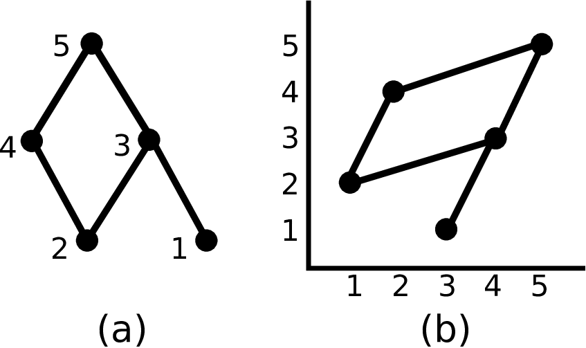
One crucial tool we use is a bijection between permutations of $n$ and two-dimensional posets with ground set $[n]$, where the labeling provided by the ground set is a linear extension (which Björner and Wachs in [4] call a natural labeling). Let ${\mathcal{P}}_{n}$ be the set of all such posets. We define $\Phi:{\mathcal{S}}_{n}\rightarrow{\mathcal{P}}_{n}$ as follows. Let $\sigma$ be a permutation of $n$, and consider $\sigma$ written in one-line notation. Interpret $\sigma$ as one chain in a realizer, reading left-to-right. For the other chain, take $[n]$ with the usual $\leq$ ordering. This realizer yields a two-dimensional poset, $\Phi(\sigma)$. As an example, consider the permutation $\sigma=24135$. To construct $\Phi(\sigma)$, we consider the realizer composed of the two chains $1\prec 2\prec 3\prec 4\prec 5$ and $2\prec 4\prec 1\prec 3\prec 5$. Their intersection gives the poset whose Hasse diagram is pictured in Figure 2 (a). Note that this poset can also be obtained from the graph of $\sigma$ as a function, as depicted in Figure 2 (b).

Some other key relationships between posets and permutations are discussed at the beginning of Section 2. This material builds toward the main result of Section 2, that $|[\sigma_{1},\sigma_{2}]|$ is polynomial-time computable whenever $\sigma_{1}^{-1}\sigma_{2}$ has bounded width. Section 3 defines intrinsic width in order to generalize the argument of Section 2 to include the more general case where $\sigma_{1}^{-1}\sigma_{2}$ has bounded intrinsic width. Finally, Section 4 applies the ideas of previous sections to random permutations.

A central question that remains is the following.

We make significant use of a result of Björner and Wachs relating the linear extensions of a two-dimensional poset to an interval in the weak Bruhat order.

The following lemma is implicit in the work of Björner and Wachs. It is stated separately here to lend clarity to subsequent proofs.

To understand this lemma, it is helpful to look at an example. The weak Bruhat order on ${\mathcal{S}}_{n}$ is shown in Figure 1. Let $\sigma=312$. Then, $\Phi(\sigma)$ has linear extensions $1\prec 2\prec 3$, $1\prec 3\prec 2$, and $3\prec 1\prec 2$. Notice that these are exactly the elements of $[\id,\sigma]$.

Before we begin considering the complexity of interval size computations, we present a simple lemma relating permutation width and poset width.

In order to extend Wei’s result on the computability of interval sizes in the weak Bruhat order, we make use of the connection between two-dimensional posets and intervals. We are able to handle a larger collection of intervals because of the following theorem about the computational complexity of linear extension counting, which was proved in previous work. This theorem is actually a weaker version of Theorem 9 in [6]. We use of the full result in Section 3 of this paper, where it appears as Theorem 13.

As stated, Theorem 4 assumes that $k$ is fixed, but we in fact need to understand the dependence of the constant in the big O on $k$. By retracing the proof of this theorem and keeping track of the constants, we obtain the following corollary.

One additional lemma allows us to generalize the previous theorem to intervals which do not necessarily contain the identity.

We now extend the results from the previous section to encompass a larger set of permutations, namely those of bounded intrinsic width. Before defining intrinsic width, we need to give some definitions related to the Gallai decomposition of a poset.

Given $P=(S,\prec)$, define a subset $T\subset S$ to be a module of $P$ if, for all $u,v\in T$ and $x\in S\setminus T$, $u\prec x$ iff $v\prec x$ and $x\prec u$ iff $x\prec v$. A module $T$ is strong if, for any module $U\subset S$, $U\cap T\neq\emptyset$ implies $U\subset T$ or $T\subset U$. Thus, the nonempty strong modules of $P$ form a tree order, called the (Gallai) modular decomposition of $P$. A strong module or poset is said to be indecomposable if its only proper submodules are singletons and the empty set. It is a result of Gallai ([8]) that the maximal proper strong modules of $P$ are a partition $\Gal(P)$ of $S$. We define the quotient poset $P/\Gal(P)$ as the poset with ground set consisting of the strong modules of $P$ and partial ordering relation defined by $T_{1}\prec T_{2}$ if and only if $t_{1}\prec t_{2}$ for some $t_{1}\in T_{1}$ and $t_{2}\in T_{2}$. For example, consider the poset $P=([9],\prec)$ shown in Figure 3 (a). The poset has four maximal proper strong modules, namely $\{1,4,5,6\}$, $\{2,3\}$, $\{7\}$, and $\{8,9\}$. (It also has the strong, but not maximal strong, module $\{4,5,6\}$.) Note that these strong modules form a partition of $P$. The quotient $P/\Gal(P)$ is shown in Figure 3 (b).

Furthermore, Gallai showed the following. The comparability graph $G(P)$ of a poset $P$ has as its vertex set the ground set of $P$ and has an edge $\{x,y\}$ for $x\neq y$ if and only if $x$ and $y$ are comparable.

Figure 3 only captures the quotient construction for the first level of the Gallai Modular Decomposition. The full decomposition (represented only as subsets without the quotient posets) is shown in figure 4.

Define the intrinsic width $\iw(P)$ of a poset as the maximum width of the posets $P|_{T}/\Gal(P|_{T})$ over all indecomposable-type nodes $T$ of the tree order given by the Gallai modular decomposition of $P$. So, for example, series-parallel posets are characterized by having intrinsic width $1$. The example given in Figure 3 has intrinsic width $2$.

To parallel the concept of poset intrinsic width, we introduce the concept of intrinsic width for permutations. First, we describe a systematic way of building permutations, which parallels the Gallai decomposition for posets. Let $\sigma\in{\mathcal{S}}_{n}$ be a permutation. Let $(\tau_{i})_{i=1}^{n}$ be a sequence of permutations with $\tau_{i}\in{\mathcal{S}}_{m_{i}}$. Define $M=\sum_{i=1}^{n}m_{i}$ and define the interval $A_{j}=[1+\sum_{i=1}^{j-1}m_{i},\sum_{i=1}^{j}m_{i}]$. Finally, we define the inflation of $\sigma$, which is denoted $\sigma[\tau_{1},\tau_{2},\ldots,\tau_{n}]$. For each $x\in A_{j}$, define

To help provide intuition for this definition, consider the following example. Let $\sigma=132$, $\tau_{1}=2314$, $\tau_{2}=12$, and $\tau_{3}=321$. Then $\sigma[\tau_{1},\tau_{2},\tau_{3}]=231489765$. This permutation is represented graphically in Figure 5, and its construction as an inflation is indicated by the three light gray boxes.

We use this notion of inflation to decompose permutations in a manner similar to the Gallai decomposition. First, we need a couple of additional definitions. Given a permutation $\pi\in{\mathcal{S}}_{n}$ a block in $\pi$ is a set of consecutive indices $\{i,i+1,\ldots,i+k\}$ such that the set of images $\{\pi(i),\pi(i+1),\ldots,\pi(i+k)\}$ is a contiguous subset of $[n]$. Note that blocks in the permutation $\pi$ correspond to intervals in the poset $\Phi(\pi)$. It is easy to see that all permutations have blocks of size $1$ and $n$. If $\pi$ has no other blocks, then it is simple. Notice that $\pi$ is simple if and only if $\Phi(\pi)$ is indecomposable. Furthermore, Albert and Atkinson have shown that the decomposition of $\pi=\sigma[\tau_{1},\tau_{2},\ldots,\tau_{k}]$ is unique in the case where $\sigma$ must be a simple permutation.

Albert and Atkinson prove this result directly by considering the blocks of $\pi$. However, the lemma can also be obtained by applying the Gallai decomposition to the two-dimensional poset $\Phi(\pi)$. Viewed in this light, the above lemma is in fact a restricted case of Theorem 10. The case where $\sigma=12$ corresponds to a series-type node, and the case where $\sigma=21$ corresponds to a parallel-type node. There is one minor disagreement between the two decompositions: Albert and Atkinson would term a monotone permutation of size more than two decomposable, whereas the Gallai decomposition tree of its corresponding poset has height only two. This is due to a slight difference in the handling of series-type and parallel-type nodes, where more than two child nodes are allowed in the Gallai decomposition, but not in the permutation block decomposition.

Like the Gallai decomposition, we can recursively apply Lemma 11 to each of $\tau_{1},\tau_{2},\ldots,\tau_{k}$ to obtain a complete block decomposition of $\pi$. Since Lemma 11 precisely corresponds to Theorem 10, for a given permutation $\pi$ the block decomposition of $\pi$ and the Gallai decomposition of $\Phi(\pi)$ have identical structure, up to the partitioning of monotone blocks.

We define intrinsic width for permutations recursively. First, any monotone permutation has intrinsic width $1$, and any simple non-monotone permutation of width $k$ has intrinsic width $k$. Then

Notice that this definition makes the set of all permutations with intrinsic width bounded by $k$ a “substitution-closed class”.

The following theorem, which is an extension of Theorem 4, bounds the computational complexity of enumerating linear extensions in the case of bounded intrinsic width.

By applying this to dimension-two posets, we obtain an extension of Wei’s result ([11]).

Thanks to well-known results on the width of random permutations, we are able to conclude that, for all but an exponentially small fraction of $\sigma\in{\mathcal{S}}_{n}$, the quantity $|[\id,\sigma]|$ can be computed with a sub-exponential time algorithm. We begin by introducing the relevant known results on random permutations. Vershik and Kerov [9], and Logan and Shepp [10] showed the following.

The following concentration result is due to Frieze.

Several similar but stronger results of this type exist, but the above theorem is sufficient for our purposes. Since permutations with an increasing subsequence of a given length are in bijection with permutations having a decreasing subsequence of the same length, we can read both of these theorems as statements about expected permutation width. Combining these results with Theorem 6 provides the following.

Of course, the previous theorem can be recast in terms of dimension two posets, demonstrating that, for large enough $n$, most two-dimensional posets with $n$ elements have a sub-exponential time algorithm which computes the number of linear extensions.

References

- [1] M.H. Albert and M.D. Atkinson. Simple permutations and pattern restricted permutations. Discrete Mathematics, 300(13):1 – 15, 2005.
- [2] Sanjeev Arora and Boaz Barak. Computational complexity: a modern approach. Cambridge University Press, 2009.
- [3] Anders Björner and Michelle L Wachs. Generalized quotients in Coxeter groups. Transactions of the American Mathematical Society, 308(1):1–37, 1988.
- [4] Anders Björner and Michelle L. Wachs. Permutation statistics and linear extensions of posets. J. Combin. Theory Ser. A, 58(1):85–114, 1991.
- [5] Graham Brightwell and Peter Winkler. Counting linear extensions. Order, 8(3):225–242, 1991.
- [6] Joshua Cooper and Anna Kirkpatrick. The complexity of counting poset and permutation patterns. arXiv preprint arXiv:1409.4368, 2014.
- [7] Alan Frieze. On the length of the longest monotone subsequence in a random permutation. Ann. Appl. Probab., 1(2):301–305, 1991.
- [8] T. Gallai. Transitiv orientierbare Graphen. Acta Math. Acad. Sci. Hungar, 18:25–66, 1967.
- [9] SV Kerov and AM Vershik. Asymptotics of the Plancherel measure of the symmetric group and the limiting form of Young tableaux. In Soviet Math. Dokl, volume 18, pages 527–531, 1977.
- [10] Benjamin F Logan and Larry A Shepp. A variational problem for random Young tableaux. Advances in mathematics, 26(2):206–222, 1977.
- [11] Fan Wei. The weak Bruhat order and separable permutations. arXiv preprint arXiv:1009.5740, 2010.