On Estimating the Perimeter Using the Alpha-Shape
Abstract
We consider the problem of estimating the perimeter of a smooth domain in the plane based on a sample from the uniform distribution over the domain. We study the performance of the estimator defined as the perimeter of the alpha-shape of the sample. Some numerical experiments corroborate our theoretical findings.
Keywords: perimeter estimation; -shape; -convex hull; rolling condition; sets with positive reach.
1 Introduction
The problem of recovering topological and geometric information about the support of a distribution based on a sample has received a considerable amount of attention in a number of fields, such as computational geometry, computer vision, image analysis, clustering or pattern recognition. This includes, for example, estimating of the number of connected components (Biau et al., 2007), the intrinsic dimensionality (Levina and Bickel, 2005) and, more generally, the homology (Niyogi et al., 2008; Carlsson, 2009; Zomorodian and Carlsson, 2005; Chazal and Lieutier, 2005; Robins, 1999), the Minkowski content (Cuevas et al., 2007a), as well as the perimeter and area (Bräker and Hsing, 1998; Rényi and Sulanke, 1964). The estimation of the support or, more generally, level sets of a density is itself a rich line of research (Polonik, 1995; Singh et al., 2009; Cadre, 2006; Tsybakov, 1997; Walther, 1997; Rodríguez Casal, 2007). A closely related topic is that of set estimation (Mammen and Tsybakov, 1995; Cuevas and Fraiman, 2010). We refer the reader to the classic book of Korostelëv and Tsybakov (1993), which treats a number of these topics.
We focus here on the problem of estimating the perimeter of the support. Concretely, we are given a set of points , which we assume are independently sampled uniformly at random from an unknown compact set , and our goal is to estimate the perimeter of , by which we mean the length of its boundary. Let denote the boundary of a set , namely , where denotes the closure of and is the complement of .
1.1 Related work
Rényi and Sulanke (1964) address this problem under the assumption that is convex and estimate its perimeter by the perimeter of the convex hull of the sample . They obtain the precise rate of convergence in expectation, which is of order when the boundary has bounded curvature. They also obtain an analogous result for the problem of estimating the area of . Bräker and Hsing (1998) extend their results to other sampling distributions. See (Reitzner, 2010) for a review on more recent results on the convex hull of a random sample.
There is a series of papers that consider the problem of estimating the surface area of the boundary of a more general class of supports but under a different sampling scheme where two samples are given, one from the uniform distribution on and another from the uniform distribution on , where is a bounded set containing . In that line, Cuevas et al. (2007b) aim at estimating the Minkowski content of , and introduce an estimator that is proved to be consistent under weak assumptions on the set . They obtain a convergence rate of in dimension 2 when has bounded curvature—in which case the Minkowski content coincides with the perimeter. Pateiro-López and Rodríguez-Casal (2009); Pateiro-López and Rodríguez-Casal (2008) follow their work and propose a different estimator, which is very closely related to the one we study here, obtaining an improved rate convergence of in dimension 2. Continuing this line of work, Jiménez and Yukich (2011) propose an estimator of the perimeter of based on a Delaunay triangulation, which is shown to be consistent under mild assumptions on .
Also closely related is the work of Kim and Korostelev (2000) in the context of binary images, which includes the estimation of the length of the boundary of a horizon of the form , where is a function with Hölder regularity. See Section 6 for further comments.
1.2 The -rolling condition
A set is said to fulfill the -rolling condition if for any there is a open ball with radius , , such that and . In this paper, we work under the assumption that satisfies the following condition:
is a compact subset of such that both and satisfy the -rolling condition.
From a geometrical point of view, we are assuming that a ball of radius can roll inside and . This rolling condition implies that, for any , there are two open balls and such that , and . In fact, it can be easily seen (Pateiro-Lopez, 2008, Lemma A.0.1) that this is only possible if there is a (unique) unit vector (the unit normal vector at pointing outward) such that and , where denotes the open ball with radius and center . See (Walther, 1999) for a comprehensive discussion, including a relation to Serra’s regular model and mathematical morphology. The -rolling condition is closely linked to the notion of -convexity. A set is said to be -convex if for any point there is a open ball of radius such that and (Perkal, 1956; Walther, 1997). It is known that, if both and satisfy the -rolling condition, then and are -convex; see (Pateiro-Lopez, 2008, Lemma A.0.8) and also (Walther, 1999).
The -rolling condition is also connected with the idea of sets of positive reach introduced in the seminal paper (Federer, 1959). For a nonempty set and , define
where stands for the Euclidean norm. The reach of a set , denoted , is the supremum over such that there is a unique point realizing on the set For twice differentiable submanifolds (e.g., curves), the reach bounds the radius of curvature from above (Federer, 1959, Lem. 4.17). Also, if and satisfy the -rolling condition then ; see (Pateiro-Lopez, 2008, Lemma A.0.6). Conversely, using results in (Cuevas et al., 2012), it follows easily that the converse is true if, in addition, is equal to the closure of its interior.
1.3 The estimator
Our estimator for the perimeter of is the perimeter of the -shape of , for some fixed . The -shape of is the polygon, denoted , whose edges—which we call -edges—are defined as follows (Edelsbrunner et al., 1983). A pair forms an -edge if there is an open ball of radius such that and . If is large enough, the -shape coincides with the convex hull of the sample. For a smaller , the -shape is not necessarily convex. See Figure 1 for an illustration. The -shape is well known in the computational geometry literature for producing good global reconstructions if the sample points are (approximately) uniformly distributed in the set . Moreover, it can be computed efficiently in time . See (Edelsbrunner, 2010) for a survey.
Cuevas et al. (2012) estimate the perimeter of by the outer Minskowski content of the -convex hull of the sample, defined as the smallest -convex set that contains the sample. Since the boundary of that set is smooth except at a finite number of points, the outer Minskowski coincides with the perimeter. See (Ambrosio et al., 2008) for a broader correspondence between these two quantities. Cuevas et al. (2012) show that this estimator is consistent, but no convergence rate is provided. Note that, for large sample sizes, both estimators are quite similar; see Proposition 2 for a formal statement. From the computational point of view, the -shape of the sample tends to be more stable with respect to the value of , and is faster to compute over a range of values of —the latter can be done in time, since the -shape changes a finite number of times with . The -convex hull of the sample does not enjoy such properties.
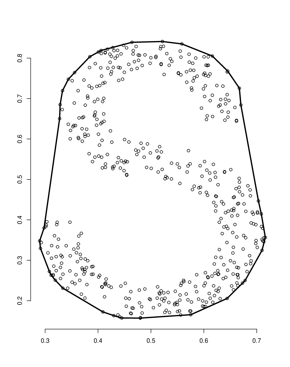
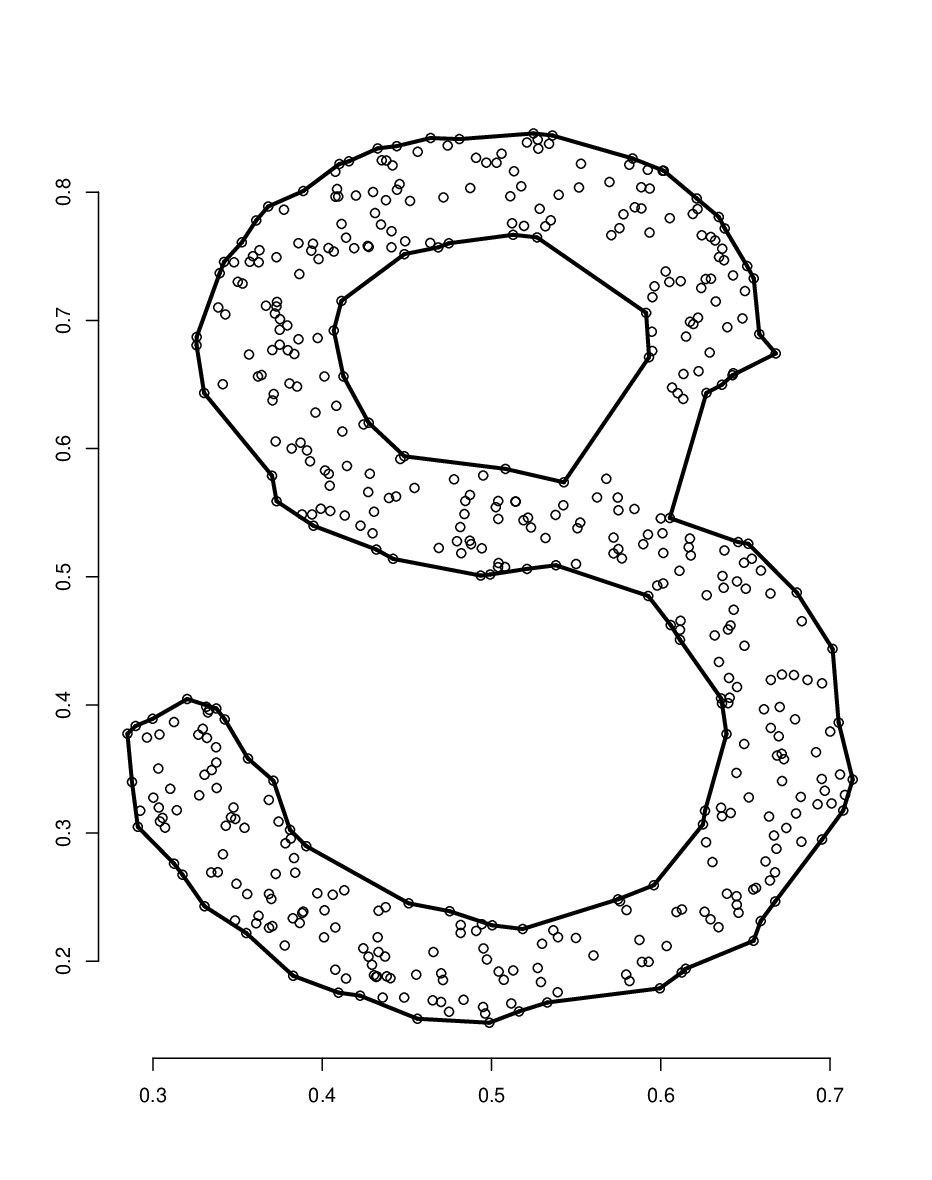
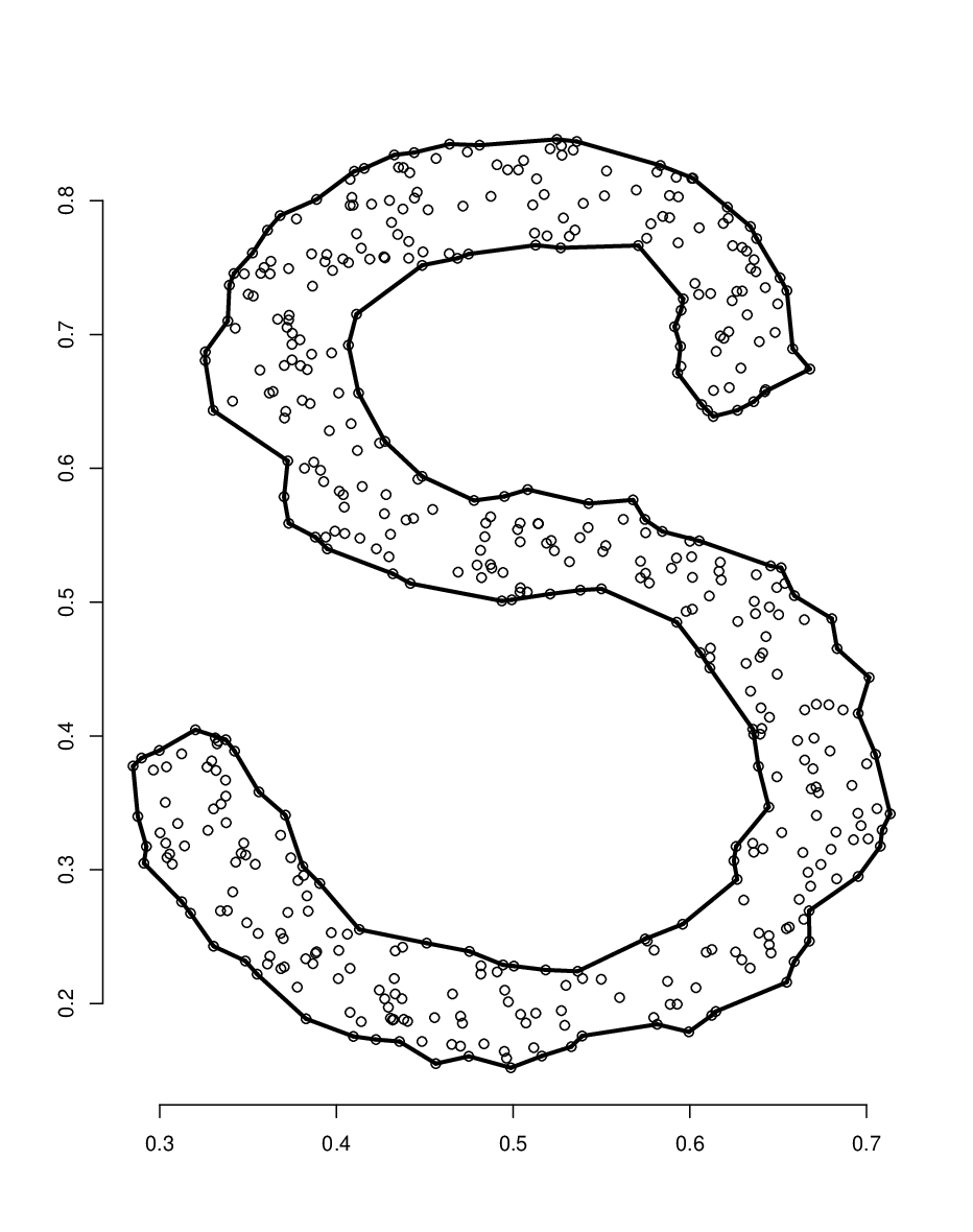
1.4 Main results
Let denote the one-dimensional Hausdorff measure in , normalized so that it equals 1 for a line segment of length 1, and let denote the diameter of a set .
Theorem 1.
Let be an independent sample from the uniform distribution on a compact set such that and satisfy the -rolling condition. Fix . There is a constant depending only on and depending only on such that, for all ,
| (1) |
Remark 1.
In particular, defining , with probability one,
eventually, by applying the Borel-Cantelli lemma. So, the convergence rate of as an estimator of is, up to a log factor, of order .
Remark 2.
We will argue later on that the same result holds also for the perimeter of the -convex hull of the sample, refining, thus, the convergence established in (Cuevas et al., 2012). See the discussion in Section 6.
1.5 Content
The remaining of the paper is largely devoted to proving Theorem 1. In Section 2 we establish some auxiliary geometrical results. Section 3 is dedicated to the study of -edges. Theorem 1 is proved in Section 4. Some numerical experiments are presented in Section 5. We discuss some extensions and open problems in Section 6.
1.6 Notation and preliminaries
We start by introducing some notation and some general concepts. Let denote the Lebesgue measure of a measurable set . For a pair of distinct points , let denote the line passing through and , and let denote the line segment with endpoints and . For a non empty set and , define
If is a singleton we use the notation (resp. ) instead of for denoting the open (resp. closed) ball of radius and center . Let denote the metric projection onto a set , i.e., , which is a singleton when . For two nonempty sets , let denote their Hausdorff distance, defined as
For a curve and , denotes the tangent subspace of at when it exists. For two curves, and , respectively differentiable almost everywhere and differentiable, and such that and , define the deviation angle of with respect to as
where denotes the angle between the tangent spaces of and at and , respectively (Morvan, 2008). Note that it is not symmetric in and .
Where they appear, and are fixed. Everywhere in the proof, a constant only depends (at most) on and the diameter of . We will leave this dependence implicit most of the time.
We let denote the sample size throughout. We say that an event holds with high probability if it happens with probability at least for some constant .
2 Some geometrical results
In this section we gather a few geometrical results that we will use later on in the paper.
Lemma 1.
Let such that and satisfy the -rolling condition. Any ball of radius with center in contains a ball of radius included in .
Proof.
Let be a shorthand for . First, we will analyze the case . If satisfies , then . Now, take such that and let be the metric projection of onto , which is well-defined since . By the -rolling property, there is an open ball of radius tangent to at that contains and . Therefore contains the ball of radius tangent to at that contains . See Figure 2 for an illustration. This concludes the proof for . If , the ball of radius contains the ball of radius with same center. By what we just did, that ball contains a ball of radius which belongs to .
4,3.5)(2,1)(0,0)(4,3.5)
∎
Recall that denotes the Lebesgue measure on .
Lemma 2.
Let be measurable and such that and satisfy the -rolling condition. For any , there is a numeric constant depending only on such that, for any ,
Proof.
Let be a shorthand for . It suffices to consider such that . Let be the metric projection of onto , which is well-defined since , and let be the open ball of radius tangent to at and contained within . It is clear that . The intersection is the union of two spherical caps symmetric with respect to line joining the two points at the intersection . See Figure 3 for an illustration. If denotes one of them, we therefore have , with a spherical cap of radius and height . Its area is equal to
Using the bound , valid for , and the bound , valid for , we obtain with .
4,3.5)(2,1)(0,0)(4,3.5)
∎
For the following result, we use some heavy machinery from the seminal work of Federer (1959). For a set , let denote its Euler-Poincaré characteristic, and recall that denotes its length.
Lemma 3.
Suppose is compact, with both and satisfying the -rolling condition. There are constants depending only on and such that and .
Proof.
Let and , and assume, without loss of generality, that . For a given such that , let denote the th curvature measure associated with , as defined in (Federer, 1959, Def. 5.7). In (Federer, 1959, Rem. 5.10) we find that
| (2) |
where is the total variation of over . Now, by (Federer, 1959, Rem. 6.14), coincides with the one-dimensional Hausdorff measure, so that . From this, we deduce the existence of . By (Federer, 1959, Th. 5.19), coincides with and, by (2) for , we get that there is some constant such that . ∎
We define an -net of a set as any subset of points such that when , and that, for any , for some . Note that any bounded set admits an -net of finite cardinality.
Lemma 4.
For any bounded , there is a constant depending only on such that, for any , any -net for has cardinality bounded by . If, in addition, both and satisfy the -rolling condition, then there is a constant depending only on and such that any -net for has cardinality bounded by .
Proof.
Assume without loss of generality that where . Let be an -net of . Since when , we have
using Lemma 1 in the last inequality. We therefore have . This proves the first part.
For the second part, let . It is enough to show the results for . Note that by the -rolling condition on . Let be an -net of . Since when , we have
| (3) |
By (Federer, 1959, Th. 5.6), we have
where (Federer, 1959, Rem. 6.14) and is the Euler-Poincaré characteristic of (Federer, 1959, Th. 5.19). By Lemma 3, there are positive constants depending only on and such that and , yielding
where , using the fact that . Plugging this into (3), we conclude the proof of the second part. ∎
Next, we establish some basic properties of a line segment joining two points on a circle which barely intersects a set with smooth boundary.
Lemma 5.
Proof.
Let be a shorthand for . Define , and let denote the canonical basis vectors of . Since , is well-defined. Without loss of generality, assume that is the origin and that the tangent of at is the line spanned by . Note that the line is perpendicular to the tangent at , so that is on the line defined by and without loss of generality we assume . Let be a shorthand for and let (resp. ) be the open ball centered at (resp. ) with radius . Since and satisfy the -rolling condition, and . Let . By construction belongs to . See Figure 4 for an illustration.
4,4.25)(2,2)(0,0)(4,4)
For any point ,
Direct calculations show that is given by the points , where
So, using the fact that , we have
| (7) |
To prove (4), take . If , then and we saw that . If , let be the closure of the intersection of with the half-plane above the line . Since and , necessarily , which in turn implies that since is convex. In particular, , so that . And since (by symmetry), we conclude with the triangle inequality that
| (8) |
for . This is valid for any , and proves (4) for any .
To prove (5), we use the fact that , so that , and when , which is the case since our assumptions that and imply , which forces by (7). Continuing, we then have
by (8). From this we get
| (9) |
where . This proves (5) for any .
We turn to proving (6). We first note that is well-defined. Indeed, by assumption , with , and , so that by (4), and we conclude with the fact that . For any we can therefore compute the point . Using the triangle inequality for angles, we have
| (10) |
We first bound . Direct trigonometric calculations show that
where the last inequality comes from (9). We use the fact that for all , we get , where . It remains to bound in (10). We have and , and by construction, and also because of (4). Hence, by (Federer, 1959, Th. 4.8(8)), we get
Using the fact that , and then (9), we have Now, if we denote by and the outward pointing unit normal vector of at and respectively, (Walther, 1997, Th. 1) ensures that
Since , we get
We arrive at
As before, this implies that , where . We conclude that
which proves (6) for any . ∎
The following is a technical result involving two line segments, one on each of two intersecting circles of same radius, and a line passing through these line segments.
Lemma 6.
Let such that , and let and . Let be any line intersecting both and . Then there is a constant depending only on such that
5,3.5)
Proof.
Let and be a shorthand for and , respectively. Since the maximum above is bounded by , it is enough to prove the inequality when
Let , and let and denote the two half-spaces defined by . Let denote the intersection point , and define analogously. Let denote the intersection point , and define analogously. See Figure 5 for an illustration.
We claim that, when , the points are either all in or all in . Indeed, when and are on opposite sides of , then either and , or and . (For two points , denotes the shorter arc defined on by and .) The distance between a point in and a point in is not smaller than the minimum of and , since . Therefore, assume without loss of generality that .
Let be the point in furthest from , so the tangent of at is parallel to . Define similarly, with in place of . We claim that and . We prove this for , without loss of generality, and consider the two possible cases:
- •
If , then
- •
If , let us define , and . By the Pythagoras theorem,
From this we get , where the inequality is due to . But . Hence, , as claimed.
By the fact that is convex, the angle between and is bounded from above by the maximum angle between and the tangent of at any point in . Moreover, by direct calculations, similar to that on Lemma 5, for any point on such that , the angle between and the tangent of at is bounded by . Hence, by the fact that , we have
Similarly,
By an analogous convexity argument, coupled with the fact that all the action is in half-space , is bounded from above by the maximum of any angle between and a tangent of at any point in , or any angle between and a tangent of at any point in . Hence, as before, we get
All the bounds combined, together with the triangle inequality, yield
and similarly for . ∎
The following result is useful when comparing the length of two curves in terms of their Hausdorff distance and their deviation angle.
Lemma 7 (Th. 43 in (Morvan, 2008)).
Let be a compact curve in such that and let be another curve in , differentiable almost everywhere, such that and is one-to-one on . Then
Proof.
The result is an immediate consequence of (Morvan, 2008, Th. 43) and the fact that the reach bounds the radius of curvature from above (Federer, 1959, Lem. 4.17). ∎
3 Some properties of -edges
Our standing assumption in this section is the following:
- ()
The data points are independently sampled from a uniformly distribution with compact support such that both and satisfy the -rolling condition.
For any pair of distinct data points within distance from each other, there are only two circles of radius passing through them, symmetric with respect to the line joining the two points. In the special case of an -edge, at least one of the two circles is empty of data points inside. The following result implies that, with probability tending to one, the center of such a circle lies outside of .
Proposition 1.
Assume ( ⋆ ) ‣ 3. For any , there is a constant depending only on such that, with probability at least , there are no open balls of radius with center in empty of data points.
Proof.
Let and assume without loss of generality that . We will focus on the case . The case can be analyzed similarly. By Lemma 1, if there is a ball of radius with center in empty of data points, then there is a ball of radius included within that is empty of data points. By Lemma 4, there is an -net of , denoted , satisfying , where depends only on and . By the triangle inequality any ball of radius included within contains a ball of the form . Hence,
where in the second inequality we used the union bound and in the third we used the fact that and . Therefore the result holds with . ∎
Remark 3.
We say that a data point is -isolated if there are no other data points within distance from it. Suppose that is -isolated so that . By the -convexity of , there is an open ball with radius such that , which in particular satisfies . Let be an open ball of radius such that . By construction, is included within and is empty of data points. We conclude by Proposition 1 that, under ( ⋆ ) ‣ 3, with high probability, there are no -isolated data points.
Proposition 2.
Take and finite set of points such that there are no -isolated points. Then the vertices of the -shape of and the vertices of the -convex hull of coincide.
Proof.
Let and denote the -shape of and the -convex hull of , respectively. Note in particular that where is the set of open balls of radius that do not intersect . First, take such that . By (Cuevas et al., 2012, Prop. 2), there is a open ball of radius such that but . Let pivot on . Since is not -isolated, the ball will eventually hit another data point, denoted . Then and belong to the boundary of an open ball of radius that does not contain any other data point by construction—for otherwise the ball would have hit that another data point before —so forms an -edge. This implies that is a vertex of . By definition of above, . Therefore , and since , we have . ∎
The next proposition bounds the expected number of -edges.
Proposition 3.
Assume ( ⋆ ) ‣ 3. For any , there is a constant depending only on such that the expected number of -edges is bounded by .
Proof.
Let and denote the number of vertices of the -shape and -convex hull, respectively, and let denote the event that there are no -isolated points. By Proposition 2, on , so that , and consequently
On the one hand, for some constant , by Proposition 1 and Remark 3. On the other hand, by (Pateiro-López and Rodríguez-Casal, 2013, Th. 3), , for some constant . From this, we conclude. ∎
Remark 4.
For , let be the event that forms an -edge. By the fact that the points are iid, is independent of . Hence, the expected number of -edges and Proposition 3 implies that for some constant .
The next result ensures that, with high probability, for each connected component of there is at least one -edge within distance .
Proposition 4.
Assume ( ⋆ ) ‣ 3. For any , there is a constant depending only on such that, with probability at least , for any connected component of , there is an -edge with an endpoint within distance of that component.
Proof.
Suppose that all the open balls of radius centered at a point in intersect the sample. By Proposition 1 this happens with probability at least for some constant . We saw in Remark 3 that this implies that there are no -isolated data points. Let be a connected component of . Fix and let denote the normal unit vector of at pointing away from . For , define and let . Notice that and, therefore, it is empty of data points. Hence, . Moreover, we also have , since we are assuming that contains at least one data point (since ). By construction, there exists a data point . Now, pivot the ball on as we did in the proof of Proposition 2. Since is not -isolated, the ball will eventually hit another data point, denoted , and will form an -edge. And, since and (remember ), there is such that . We now use the fact that is contractible (Federer, 1959, Rem. 4.15), and since , we must have , which in turn implies that and, therefore, . ∎
Next, we prove some quantitative results about -edges. In plain English, we show that, with probability tending to one, -edges are near the boundary of , have small length and their deviation angle with the boundary of is small.
Proposition 5.
Assume ( ⋆ ) ‣ 3. For , let denote the event that is an -edge, and for , let denote the event that
| (11) |
For any , there is a constant depending only on such that, for any , .
Proof.
Let be a shorthand for . For any two distinct points such that , define
where and denotes the rotation at angle . By construction, , and are the only two points with this property. Let be short for , if , and , otherwise.
Let be the event that there are no open balls of radius with center in empty of data points. We studied this event in Proposition 1. With denoting the constant of Lemma 5, we have
Therefore, the union bound gives
With denoting the constant of Lemma 2, for any deterministic point such that , we have
for some constant which depends only on and . Hence, conditioning on , we have
Together with Proposition 1, we arrive at
for some constant , again depending only on . ∎
The next two results combined imply that, with high probability, the -edges form a simple polygon in one-to-one correspondence with . The first result shows that, with high probability, two distinct points in the union of all -edges do not project on the same point on . We also show that -edges are all one-sided in the sense that at least one of the two open balls of radius that circumscribes an -edge contains a data point.
Proposition 6.
Assume ( ⋆ ) ‣ 3. For any , there is a constant depending only on such that, with probability at least : (i) all -edges are one-sided; and (ii) the metric projection onto is injective on the union of all -edges.
Proof.
Let be a shorthand for and . Assume there are no balls of radius with center in empty of data points and that, for fixed (and chosen small enough in what follows), all the -edges satisfy (11). Both events happen together with probability at least , for some constant , by Propositions 1 and 5.
We first show that, if is small enough, all -edges are one-sided. Let () be an arbitrary -edge. Let be the midpoint of that -edge and . If there is a ball of radius , , such that , then the center of is either or , where is the unit vector orthogonal to such that , being the outward pointing unit normal vector at , which is well-defined when . Notice that the vector is well defined when , since in that case is not orthogonal to . We will prove that, for even smaller, and therefore is not empty of sample points. Define and . By the -rolling property, . By the triangle inequality and (11), we have
with, for small enough,
using (11) (i.e., ) and the fact that for any . Using the triangle inequality and (11), again, we get
for small enough, in which case .
Now we prove that the metric projection onto is injective on the union of all -edges. Indeed, assume that this is not the case, so there are two distinct points belonging to some (necessarily distinct) -edges, and , with the same metric projection onto , denoted . Let be the outward pointing unit normal vector at . For short, let , , , . By the triangle inequality and the fact that , and then (11), we have
| (12) |
when is small enough. Also by the triangle inequality for angles and (11),
| (13) |
Let and denote the open balls of radius circumscribing and , respectively, and empty of data points. Since all -edges are one-sided, these balls are uniquely defined. Also, define and analogously to and above, but based on and , instead of and . Using the same notation as above, we have and and
| (14) |
Reasoning as in (12) above, we have . Also,
Using (11), and, similarly, . Moreover, by (13) and using again the inequality for any , we get . Hence,
Hence, the bound in (14) leads to when is small enough, where is a constant. Combining this bound with that in (13), and applying Lemma 6, we obtain that
where is a constant. By the fact that is parallel to (Federer, 1959, Th. 4.18(12)) and using (11), we also have
We therefore have a contradiction when is small enough that all the derivations above apply and, in addition, . ∎
Remark 5.
Any one-sided -edge shares each one of its endpoints with another -edge. Indeed, suppose is an -edge, so that there exists such that and . In that case, let pivot on , as we did in the proof of Proposition 4 away from . Let denote the first data point that the ball hits. Then is an -edge by construction. If is not shared with any other -edge, then the ball pivots on away from until it touches from the other side. That (open) ball is empty of data points inside, and together with the ball we started with, makes two-sided.
Proposition 7.
Assume ( ⋆ ) ‣ 3. For any , there is a constant depending only on such that, with probability at least , the union of all -edges is in one-to-one correspondence with via the metric projection onto .
Proof.
Let be a shorthand for and , and let denote the union of all -edges. Since is a (compact) one dimensional manifold (Walther, 1999), it is well-known that each connected component of is a closed curve homeomorphic to the unit circle, see (Lee, 2011, Thm. 5.27). We prove that this is also the case for each connected component of . We assume that the metric projection onto , meaning , is injective on , that all -edges are one-sided, that —so that is well-defined on —and that for any connected component of . This event happens with probability at least for some constant , by Propositions 5, 4 and 6. We prove that, under these circumstances, is in one-to-one correspondence with via . Indeed, let be a connected component of . Let be an -edge such that . By assumption, there is a data point such that is also an -edge. Having constructed , let be a data point such that is an -edge. Since —where the union is of disjoint sets by (Federer, 1959, Rem. 4.15, (1))— and the polygon is connected, necessarily, . Also, since the sequence is made of finitely many data points, and for all , there is such that , and we further may assume that are all distinct. Therefore, by construction, is a simple polygon made of -edges such that . In particular, the latter implies that , and since is homeomorphic to the unit circle and is continuous and injective on , is also homeomorphic to the unit circle. This forces , due to being homeomorphic to the unit circle too. Since all this is true for any , meaning any connected component of , we conclude therefore that is not only injective, but also surjective. ∎
4 Proof of Theorem 1
We are now in a position to prove the main result, meaning, Theorem 1. Let be a shorthand for and let denote the union of all -edges.
By Proposition 5 together with the union bound, and then Proposition 7, for any , with probability at least , for some constant depending only on , is in one-to-one correspondence with via the metric projection onto , and satisfies and . Note that, because and are in one-to-one correspondence, implies that , so that . We now apply Lemma 7, combined with the simple bounds , for , and , valid when . Assuming , this yields
and
We get
Hence, if , we have
Then a change of variable concludes the proof of Theorem 1.
5 Numerical experiments
In order to numerically check the conclusions of Theorem 1 we performed a small simulation study. For the set we chose the corona . In this case the value of is equal to (the radius of the hole) and . The selected sample sizes were . For each sample size , we simulated samples from the uniform distribution on and calculated the -shape for each sample. The values of were , and the limit case . Given , , and sample , we computed the sample -shape, denoted , using the R-package alphahull of Pateiro-López and Rodrıguez-Casal (2010), and then its perimeter . We estimated the expected error and bias by
respectively. Let denote the sample standard deviation of .
- •
Among the ’s that we tried, the estimator performs best at . It does not seem that, asymptotically, the best converges to . For instance, the ratio is around 6.7 for .
- •
Figure 6 shows the error versus sample size in log-log scale for . It can be seen that the error corresponding to does no go to zero whereas always outperform the other considered values of . The trend for large values of is clearly linear and the slope is close to as Theorem 1 predicts. This is particularly true when (our best choice), where fitting a line by least squares yields a slope of , with (Student) 95%-confidence interval of , and an R-squared exceeding 0.99.
- •
For the limit case , the bias, does not go to zero as the sample size increases. The error is approximately equal to 0.18; see Figure 6. This shows, from the numerical point of view, that the perimeter of the -shape is not a consistent estimator of the for . The main problem here is that the length of the -edges does not go to zero, as Proposition 5 states for .
- •
The convergence rate of the standard deviation seems to be higher that . In fact, we have reasons to believe that the slope is of order . This is confirmed numerically. Indeed, if we fit a line to the log-log plot of , we get a slope with (Student) 95%-confidence interval of . So, asymptotically, it seems that the error is dominated by the bias. This suggests that reducing the bias of the estimator could lead to improve the convergence rate of the method.
- •
The random variable seems to be asymptotically normal. For the greatest considered , the sample passes the Shapiro-Wilks normality test for several values of . For instance, for , we got a p-value of 0.82.
6 Discussion
We discuss a number of extensions and open problems.
Extensions. Our arguments extend more or less trivially to other sampling distributions. It is completely straightforward to see that Theorem 1 applies verbatim to a sampling distribution which has a density with respect to the uniform distribution which is bounded away from zero near the boundary of . A little less obvious is an extension to the case where this density converges to zero at some given rate near the boundary, which ends up impacting the rate of convergence of our estimator. In any case, our estimator remains consistent. The same results carry over to the case where has a finite number of ‘kinks’, i.e., points where the reach is infinite.
Choice of tuning parameter. The estimator depends on knowledge of , or at least a lower bound on , since any fixed appears to yield the convergence rate in . Choosing automatically, therefore, requires an estimate on the size of . This is done in recent work by Rodríguez-Casal and Saavedra-Nieves (2014). Suppose we have an estimator such that with high probability. We speculate that the convergence bound obtained in Theorem 1 with chosen equal to remains valid, albeit with a different multiplicative constant.
Finer asymptotics. Bräker and Hsing (1998) were able to compute the exact asymptotic expected value and variance of the perimeter of the convex hull of a sample, and also to show an asymptotic normal limit. An open problem would be to do the same here. Our numerical experiments lead us to speculate that our estimator is also normal in the large-sample limit.
Minimax rate. We conjecture that the rate that our estimator achieves, i.e., , is not minimax optimal, not even in the exponent. Indeed, we learn in (Korostelëv and Tsybakov, 1993, Chap 8) that for the problem of estimating the area (in the context of binary images), an estimator obtained from computing the area of an optimal set estimator (for the symmetric difference metric, and the -convex hull is such an estimator) only achieves the rate , while the optimal rate is with the assumptions we make here. It is very reasonable to infer that the same is true for the more delicate problem of perimeter estimation. In fact, Kim and Korostelev (2000) show that is (up to a poly-logarithmic factor) the minimax rate for perimeter estimation of a horizon (also in the context of binary images).
Higher dimensions. Our setting is that of a set in two dimensions. How about higher dimensions? The problem would be to estimate the -volume of the boundary of a set , under the same conditions, and the estimator would be the -volume of the -shape of , which is the union of all the -faces. We say that form an -face if they are affine-independent and there is an open ball of radius such that and . Most of the auxiliary lemmas and propositions can be extended to the general framework. However, we have no idea how to extend Proposition 7.
The -convex hull. Our results apply to the -convex hull of the sample. This is because, with high probability, it shares the same vertices as the -shape (by Proposition 2). When this is the case, the former is the union of arcs of radius with base the -edges. In particular, if an -edge is of length , then the length of that arc is . By Proposition 5 and an application of the union bound, the largest -edge is of order . We conclude that the ratio between the perimeters of the -convex hull and of the -shape is of order . We note, however, that the perimeter of the -convex hull is consistent while the perimeter of the -shape is not necessarily so. Our results require .
Acknowledgements
EAC was partially supported by a grant from the US National Science Foundation (DMS-0915160). ARC was partially supported by Project MTM2008–03010 and MTM2013-41383-P from the Spanish Ministry of Science and Innovation, and by the IAP network StUDyS (Developing crucial Statistical methods for Understanding major complex Dynamic Systems in natural, biomedical and social sciences) of the Belgian Science Policy.
References
- Ambrosio et al. (2008) Ambrosio, L., A. Colesanti, and E. Villa (2008). Outer minkowski content for some classes of closed sets. Mathematische Annalen 342(4), 727–748.
- Biau et al. (2007) Biau, G., B. Cadre, and B. Pelletier (2007). A graph-based estimator of the number of clusters. ESAIM Probab. Stat. 11, 272–280.
- Bräker and Hsing (1998) Bräker, H. and T. Hsing (1998). On the area and perimeter of a random convex hull in a bounded convex set. Probab. Theory Related Fields 111(4), 517–550.
- Cadre (2006) Cadre, B. (2006). Kernel estimation of density level sets. J. Multivariate Anal. 97(4), 999–1023.
- Carlsson (2009) Carlsson, G. (2009). Topology and data. Bull. Amer. Math. Soc. (N.S.) 46(2), 255–308.
- Chazal and Lieutier (2005) Chazal, F. and A. Lieutier (2005). Weak feature size and persistant homology: computing homology of solids in from noisy data samples. In Computational geometry (SCG’05), pp. 255–262. New York: ACM.
- Cuevas and Fraiman (2010) Cuevas, A. and R. Fraiman (2010). Set estimation. In New perspectives in stochastic geometry, pp. 374–397. Oxford: Oxford Univ. Press.
- Cuevas et al. (2012) Cuevas, A., R. Fraiman, and B. Pateiro-López (2012). On statistical properties of sets fulfilling rolling-type conditions. Adv. Appl. Probab. 44(2), 311–329.
- Cuevas et al. (2007a) Cuevas, A., R. Fraiman, and A. Rodríguez-Casal (2007a). A nonparametric approach to the estimation of lengths and surface areas. Ann. Statist. 35(3), 1031–1051.
- Cuevas et al. (2007b) Cuevas, A., R. Fraiman, and A. Rodríguez-Casal (2007b). A nonparametric approach to the estimation of lengths and surface areas. Ann. Statist. 35(3), 1031–1051.
- Edelsbrunner (2010) Edelsbrunner, H. (2010). Alpha shapes-a survey. Tessellations in the Sciences.
- Edelsbrunner et al. (1983) Edelsbrunner, H., D. G. Kirkpatrick, and R. Seidel (1983). On the shape of a set of points in the plane. IEEE Trans. Inform. Theory 29(4), 551–559.
- Federer (1959) Federer, H. (1959). Curvature measures. Trans. Amer. Math. Soc. 93, 418–491.
- Jiménez and Yukich (2011) Jiménez, R. and J. E. Yukich (2011). Nonparametric estimation of surface integrals. Ann. Statist. 39(1), 232–260.
- Kim and Korostelev (2000) Kim, J.-C. and A. Korostelev (2000). Estimation of smooth functionals in image models. Mathematical Methods of Statistics 9(2), 140–159.
- Korostelëv and Tsybakov (1993) Korostelëv, A. P. and A. B. Tsybakov (1993). Minimax theory of image reconstruction, Volume 82 of Lecture Notes in Statistics. New York: Springer-Verlag.
- Lee (2011) Lee, J. M. (2011). Introduction to topological manifolds (Second ed.), Volume 202 of Graduate Texts in Mathematics. New York: Springer.
- Levina and Bickel (2005) Levina, E. and P. Bickel (2005). Maximum likelihood estimation of intrinsic dimension. In Advances in Neural Information Processing Systems, Volume 17, pp. 777–784. Cambridge, Massachusetts: MIT Press.
- Mammen and Tsybakov (1995) Mammen, E. and A. B. Tsybakov (1995). Asymptotical minimax recovery of sets with smooth boundaries. Ann. Statist. 23(2), 502–524.
- Morvan (2008) Morvan, J.-M. (2008). Generalized Curvatures. Springer Publishing.
- Niyogi et al. (2008) Niyogi, P., S. Smale, and S. Weinberger (2008). Finding the homology of submanifolds with high confidence from random samples. Discrete Comput. Geom. 39(1-3), 419–441.
- Pateiro-Lopez (2008) Pateiro-Lopez, B. (2008). Set estimation under convexity type restrictions. Ph. D. thesis, Universidad de Santiago de Compostela.
- Pateiro-López and Rodríguez-Casal (2008) Pateiro-López, B. and A. Rodríguez-Casal (2008). Length and surface area estimation under smoothness restrictions. Adv. in Appl. Probab. 40(2), 348–358.
- Pateiro-López and Rodríguez-Casal (2009) Pateiro-López, B. and A. Rodríguez-Casal (2009). Surface area estimation under convexity type assumptions. J. Nonparametr. Stat. 21(6), 729–741.
- Pateiro-López and Rodrıguez-Casal (2010) Pateiro-López, B. and A. Rodrıguez-Casal (2010). Generalizing the convex hull of a sample: The r package alphahull. Journal of Statistical software 34(5), 1–28.
- Pateiro-López and Rodríguez-Casal (2013) Pateiro-López, B. and A. Rodríguez-Casal (2013). Recovering the shape of a point cloud in the plane. TEST 22(1), 19–45.
- Perkal (1956) Perkal, J. (1956). Sur les ensembles -convexes. Colloq. Math. 4, 1–10.
- Polonik (1995) Polonik, W. (1995). Measuring mass concentrations and estimating density contour clusters—an excess mass approach. Ann. Statist. 23(3), 855–881.
- Reitzner (2010) Reitzner, M. (2010). Random polytopes. In New perspectives in stochastic geometry, pp. 45–76. Oxford: Oxford Univ. Press.
- Rényi and Sulanke (1964) Rényi, A. and R. Sulanke (1964). Über die konvexe Hülle von zufällig gewählten Punkten. II. Z. Wahrscheinlichkeitstheorie und Verw. Gebiete 3, 138–147 (1964).
- Robins (1999) Robins, V. (1999). Towards computing homology from finite approximations. In Proceedings of the 14th Summer Conference on General Topology and its Applications (Brookville, NY, 1999), Volume 24, pp. 503–532.
- Rodríguez Casal (2007) Rodríguez Casal, A. (2007). Set estimation under convexity type assumptions. Ann. Henri Poincaré 43(6), 763–774.
- Rodríguez-Casal and Saavedra-Nieves (2014) Rodríguez-Casal, A. and P. Saavedra-Nieves (2014). A fully data-driven method for estimating the shape of a point cloud. arXiv:1404.7397.
- Singh et al. (2009) Singh, A., C. Scott, and R. Nowak (2009). Adaptive Hausdorff estimation of density level sets. Ann. Statist. 37(5B), 2760–2782.
- Tsybakov (1997) Tsybakov, A. B. (1997). On nonparametric estimation of density level sets. Ann. Statist. 25(3), 948–969.
- Walther (1997) Walther, G. (1997). Granulometric smoothing. The Annals of Statistics 25(6), pp. 2273–2299.
- Walther (1999) Walther, G. (1999). On a generalization of Blaschke’s rolling theorem and the smoothing of surfaces. Math. Methods Appl. Sci. 22(4), 301–316.
- Zomorodian and Carlsson (2005) Zomorodian, A. and G. Carlsson (2005). Computing persistent homology. Discrete Comput. Geom. 33(2), 249–274.