跳到论文正文
W Papers独立论文阅读器 arXiv:1507.00001 论文正文 计算阅读时间 · 0%
引用这篇论文根据当前论文元数据生成,正式投稿前建议核对。


License: arXiv.org perpetual non-exclusive license
arXiv:1507.00001v1 [physics.bio-ph] 29 Jun 2015

A multi-pathway model for Photosynthetic reaction center

M. Qin1,2, H. Z Shen1,2, and X. X. Yi2 Note: Corresponding address: yixx@nenu.edu.cn Affiliation: 1School of Physics and Optoelectronic Technology
Dalian University of Technology, Dalian 116024, China
2Center for Quantum Sciences and School of Physics, Northeast Normal University, Changchun 130024, China
Abstract

Charge separation in light-harvesting complexes occurs in a pair of tightly coupled chlorophylls at the heart of photosynthetic reaction centers of both plants and bacteria. Recently it has been shown that quantum coherence can, in principle, enhance the efficiency of a solar cell, working like a quantum heat engine (QHE). Here, we propose a biological quantum heat engine (BQHE) motivated by Photosystem II reaction center (PSII RC) to describe the charge separation. Our model mainly considers two charge-separation pathways more than that in the published literature. The two pathways can interfere via cross-couplings and work together to enhance the charge-separation yields. We explore how these cross-couplings increase the current and voltage of the charge separation and discuss the advantages of multiple pathways in terms of current and power. The robustness of the BQHE against the charge recombination in natural PSII RC and dephasing induced by environments is also explored, and extension from two pathways to multiple pathways is made. These results suggest that nature-mimicking architectures with engineered multiple pathways for charge separations might be better for artificial solar energy devices.

pacs
42.50.Gy, 42.50.Nn, 84.60.Jt, 82.39.Jn

I Introduction

Photosynthesis begins with the absorption of a photon which creates an excited state on a pigment molecule. The excitation is transferred between the pigments of light-harvesting complexes until it arrives at a reaction center (RC) in the pigment-protein complex, where the photon energy is used for the later dark stages of charge separation and conversion of energy from physical into chemical one. The efficiency of the energy transfer is very high, with a near unity yield [1]. This sparks the long-standing and increasing interest in the understanding of the physics behind the energy conversion within photosynthesis [2]. Recently, much attention has been paid to the role of quantum coherence: growing experimental evidence [3, 4, 5, 6, 7, 8, 9] and theoretical models [10, 11, 12, 13, 14, 15, 16, 17, 18, 19, 20, 21, 22] reveal that quantum coherence contributes beneficially to the high efficiency. Understanding the underlying mechanism of such natural system can assist us in designing novel nanofabricated structures for quantum transport and optimized solar cells.

Viewing the photosynthetic reaction center as a quantum heat engine (QHE), the authors of Ref.[23] analyzed the charge separation in light-harvesting complexes. This treatment bridges the two seemingly unrelated effects attributed to quantum coherence in natural(photosynthesis) and artificial(photovoltaics) light-harvesting systems. The common ground between photovoltaics and photosynthesis has also been investigated recently in [24, 25]. In analogy with a continuous Carnot-like cycle, Dorfman e​tet a​l.al. showed that the power of a photocell based on Photosystem II reaction center (PSII RC) can be increased by 27%27\% attributed to noise-induced quantum coherence—Fano interference [26, 27], which was found in artificial photocells and lasing without inversion. Creatore e​tet a​l.al. proposed the other mechanism and showed that the dipole-dipole interaction between two neighboring electron donors play a key role in enhancing the current and power of the photocell [28]. They claimed that this increasing can be up to 35%35\%.

In these studies, only one charge-separation pathway is considered. Identifying the primary electron donors and dominating charge-separation pathways has been a question of recent extensive research and debate. At the moment, there is much evidence that two main pathways make significant contribution under ambient condition [29, 30, 31, 32]. This motivates us to ask the question that whether a multi-pathway scheme is more beneficial to designing artificial light-harvesting devices? In this paper, we will answer this question via numerical simulation for the current and power as well as the robustness of the current and power against the charge recombination and dephasing.

The remainder of the paper is organized as follows. In Sec. II, we introduce a model of a quantum heat engine inspired by PSII RC to describe the charge separation, which includes a second pathway in comparison with the model proposed in [23, 28]. A master equation describing the evolution of the two-pathway system is also derived in this section. In Sec. III, the concepts of effective voltage VV and power are introduced and used to characterize the charge separation, new results due to the second pathway are discussed. In Sec. IV, we focus on how the multiple pathways affect the behavior of j−Vj-V and P−VP-V features. We explain the advantage of multiple pathways over simply increasing the decay rates and cross-couplings. In Sec. V, we take the charge recombination and dephasing that might coexist in natural PSII RC into consideration. Numerical results of one- and multi-pathway models are shown, from which we further see the advantage of multiple pathways. Sec. VI is devoted to concluding remarks.

II Model

To present the model, we first illustrate the structure of the Photosystem II reaction center complex in Fig. 1. The six pigment

Refer to caption
Figure 1: (Color online) Arrangement of six core-pigments in the PSII RC. It consists of the special pair PD1{{\rm{P}}_{{\rm{D1}}}}, PD2{{\rm{P}}_{{\rm{D2}}}}, the two accessory chlorophylls AccD1{\rm{Ac}}{{\rm{c}}_{{\rm{D1}}}}, AccD2{\rm{Ac}}{{\rm{c}}_{{\rm{D2}}}}, and the two pheophytins PheD1{\rm{Ph}}{{\rm{e}}_{{\rm{D1}}}}, PheD2{\rm{Ph}}{{\rm{e}}_{{\rm{D2}}}}.
Refer to caption
Figure 2: (Color online) Schemes of the BQHE model based on the photosynthetic reaction center. HTR denotes the high-temperature photon reservoir, while LTR1 and LTR2 stand for the low-temperature phonon reservoirs. HTR induces transition from the ground state |b⟩\left|b\right\rangle to the single-exciton states |a1⟩\left|{{a_{1}}}\right\rangle and/or |a2⟩\left|{{a_{2}}}\right\rangle. LTR1 induces transition from |a1⟩\left|{{a_{1}}}\right\rangle and/or |a2⟩\left|{{a_{2}}}\right\rangle to the charge-separated state |α⟩\left|\alpha\right\rangle (|α1⟩\left|{{\alpha_{1}}}\right\rangle and |α2⟩\left|{{\alpha_{2}}}\right\rangle for (b), |αi⟩\left|{{\alpha_{i}}}\right\rangle (i=1,2,3​…i=1,2,3...) for (c)). LTR2 induces transition from the ionized state |β⟩\left|\beta\right\rangle (|β1⟩\left|{{\beta_{1}}}\right\rangle and |β2⟩\left|{{\beta_{2}}}\right\rangle for (b), |βi⟩\left|{{\beta_{i}}}\right\rangle (i=1,2,3​…i=1,2,3...) for (c)) to the ground state. The three models differ in the number of donor, i.e., pathway.

molecules are closely spaced in particular positions and orientations, and coupled by the dipole-dipole interactions resulting in exciton states. These pigments are distributed in two branches of protein matrix: D​1D1 and D​2D2. PD​1P_{D1} and PD​2P_{D2}, a special pair of coupled chlorophylls, is located at the center of the PSII RC. They contribute mostly to the lowest energy states and are the primary electron donors, forming two exciton states which are denoted as |a1⟩\left|{{a_{1}}}\right\rangle and |a2⟩\left|{{a_{2}}}\right\rangle. These two pairs of molecules are also coupled to the accessory chlorophylls A​c​cD​1Acc_{D1} and A​c​cD​2Acc_{D2} located in the two different branches D​1D1 and D​2D2, respectively. P​h​eD​1Ph{e_{D1}} and P​h​eD​2Ph{e_{D2}} are the remaining two pheophytin pigments coupled to the rest of the molecules, and act as the electron acceptors. Photosynthetic antennae transfer energy of the absorbed solar photons to the RC where the transmembrane charge separation takes place. Charge separation in the core of pigment-protein RC complexes is the first energy conversion step in photosynthesis. The consequent electrochemical potential drives a chain of chemical reactions, including the reduction of NADP to NADPH, the synthesis of ATP and the oxidized part of the RC splits water, releasing molecular oxygen, all these leading eventually to the stable storage of solar energy.

The photosynthetic reaction center may be analyzed as a biological quantum heat engine(BQHE) that transforms high-energy thermal photon radiation into low-entropy electron flux. As shown in Fig. 2 (a), a five-level QHE scheme describes the photoinduced charge separation between the donor and the acceptor molecules interacting with thermal light. State |b⟩\left|b\right\rangle represents the lowest energy configuration in which both donors and acceptor molecules are in the ground state. States |a1⟩\left|{{a_{1}}}\right\rangle and |a2⟩\left|{{a_{2}}}\right\rangle correspond to single-exciton states in the first and second donors, respectively. |α⟩\left|\alpha\right\rangle is the charge-separated state with the excited electron transferred from the donors to the acceptor molecules. And |β⟩\left|\beta\right\rangle describes the ionized state in which the system is positively charged (the excited electron is assumed to have been used to perform work). The heat engine cycle begins with the excited electron promoted from |b⟩\left|b\right\rangle to |a1⟩\left|{{a_{1}}}\right\rangle and/or |a2⟩\left|{{a_{2}}}\right\rangle after the absorption of a solar photon. This excited electron is then transferred to the acceptor by emission of a phonon (transition from |a1⟩\left|{{a_{1}}}\right\rangle and/or |a2⟩\left|{{a_{2}}}\right\rangle to |α⟩\left|\alpha\right\rangle, corresponding to the formation of a radical pair PD​2+​A​c​cD​2−P_{D2}^{+}Acc_{D2}^{-} in Fig. 1). Furthermore, the electron can be released from state |α⟩\left|\alpha\right\rangle with a rate Γ\Gamma, resulting in a current from |α⟩\left|\alpha\right\rangle to |β⟩\left|\beta\right\rangle driving a chain of chemical reactions, leading eventually to the stable storage of solar energy. The current j=e​Γ​ρα​αj=e\Gamma{\rho_{\alpha\alpha}} is thus determined by the relaxation rate Γ\Gamma and the population of |α⟩\left|\alpha\right\rangle. The acceptor-to-donor charge recombination represented by the decay rate Γα→b=χ​Γ{\Gamma_{\alpha\to b}}=\chi\Gamma, with χ\chi a dimensionless fraction, brings the system back to the ground state |b⟩\left|b\right\rangle but does not produce current, limiting the power output of our QHE [28, 33]. Finally, to complete the cycle, we allow another population transfer to take place, emitting a phonon with excess energy, bringing the electron back to the neutral ground state |b⟩\left|b\right\rangle with a rate Γc{\Gamma_{c}}. We also assume that the donor excited states |a1⟩\left|{{a_{1}}}\right\rangle and |a2⟩\left|{{a_{2}}}\right\rangle undergo a dephasing process (via a rate Γd​e​p{\Gamma_{dep}}), which will influence the current and power generated. This model including one charge-separation pathway (|α⟩→|β⟩\left|\alpha\right\rangle\to\left|\beta\right\rangle) can exhibit noise-induced quantum coherence due to Fano interference, which originates from the coupling of two levels to a common reservoir and thus the effect can be revealed by the cross-couplings. Fano interference can minimize the acceptor-to-donor charge recombination by inducing coherence between |a1⟩\left|{{a_{1}}}\right\rangle and |a2⟩\left|{{a_{2}}}\right\rangle. This brings about enhanced current and power output as we will show in section II.

Although electron transfer in the PSII RC has been thoroughly investigated and several charge-separation pathways that involve the formation of several different radical pairs were identified, works on the effect of multiple charge-separation pathways are rarely found. At the moment, much evidence shows that two main pathways make significant contributions under ambient conditions [29, 30, 31, 32]. Therefore we emphatically study two pathways, i.e., we add another acceptor molecule that consists of a charged-separated state and an ionized state to the model in Fig. 2 (a). As shown in Fig. 2 (b), the initial excitation of states |a1⟩\left|{{a_{1}}}\right\rangle and |a2⟩\left|{{a_{2}}}\right\rangle can be transferred to the two acceptor molecules in states |α1⟩\left|{{\alpha_{1}}}\right\rangle and |α2⟩\left|{{\alpha_{2}}}\right\rangle, respectively, with the excess energy radiated as a phonon, and further produce electric current and returning back to |b⟩\left|b\right\rangle via |β1⟩\left|{{\beta_{1}}}\right\rangle and/or |β2⟩\left|{{\beta_{2}}}\right\rangle. Here, the total current in the two pathways is given by j=e​Γ1​ρα1​α1+e​Γ2​ρα2​α2j=e{\Gamma_{1}}{{\rho}_{{\alpha_{1}}{\alpha_{1}}}}+e{\Gamma_{2}}{{\rho}_{{\alpha_{2}}{\alpha_{2}}}}. The structures of RCs from green plants, algae, and bacteria differ in the nature and precise orientation of the constituent pigments, resulting in different spectroscopic and dynamical parameters. Nevertheless, our six-level scheme may be applied to all RCs as discussed below.

With this knowledge, the dynamics of our heat engine can be described by the following master equation,

d​ρ^Sd​t=−i⁡[HS,ρ^S]+L​ρ^S,\displaystyle\frac{{d{{\hat{\rho}}_{S}}}}{{dt}}=-i[{H_{S}},{{\hat{\rho}}_{S}}]+L{{\hat{\rho}}_{S}}, (1)

where HS=∑j=b,a1,a2,α1,α2,β1,β2Ej|j⟩⟨j|{H_{S}}=\sum\limits_{\scriptstyle j=b,{a_{1}},{a_{2}},\hfill\atop\scriptstyle{\alpha_{1}},{\alpha_{2}},{\beta_{1}},{\beta_{2}}\hfill}{{E_{j}}\left|j\right\rangle\left\langle j\right|} is the system Hamiltonian, with Ej{{E_{j}}} the energy of the iith level. The superoperator LL describing the effect of reservoirs and acceptor-donor recombinations can be decomposed as

L​ρ^S=Lh​ρ^S+Lc​1​ρ^S+Lc​2​ρ^S+Lr​e​l​ρ^S+Ld​e​p​ρ^S+Lr​e​c​ρ^S.\displaystyle\begin{aligned} L{{\hat{\rho}}_{S}}=&{L_{h}}{{\hat{\rho}}_{S}}+{L_{c1}}{{\hat{\rho}}_{S}}+{L_{c2}}{{\hat{\rho}}_{S}}+{L_{rel}}{{\hat{\rho}}_{S}}\\ &+{L_{dep}}{{\hat{\rho}}_{S}}+{L_{rec}}{{\hat{\rho}}_{S}}.\end{aligned} (2)

For the high temperature photon reservoir (HTR), its effects can be described by

Lh​ρ^S=∑k,l=1,2γk​l​h2[(nh+1)(σh​lρ^Sσh​k†+σh​kρ^Sσh​l†OPEN−σh​l†​σh​k​ρ^S−ρ^S​σh​k†​σh​l)+nh​(σh​k†​ρ^S​σh​lCLOSE+σh​l†ρ^Sσh​k−σh​kσh​l†ρ^S−ρ^Sσh​lσh​k†)],\displaystyle\begin{aligned} {L_{h}}{{\hat{\rho}}_{S}}=&\sum\limits_{k,l=1,2}{\frac{{{\gamma_{klh}}}}{2}}[({n_{h}}+1)({\sigma_{hl}}{{\hat{\rho}}_{S}}\sigma_{hk}^{\dagger}+{\sigma_{hk}}{{\hat{\rho}}_{S}}\sigma_{hl}^{\dagger}\\ &-\sigma_{hl}^{\dagger}{\sigma_{hk}}{{\hat{\rho}}_{S}}-{{\hat{\rho}}_{S}}\sigma_{hk}^{\dagger}{\sigma_{hl}})+{n_{h}}(\sigma_{hk}^{\dagger}{{\hat{\rho}}_{S}}{\sigma_{hl}}\\ &+\sigma_{hl}^{\dagger}{{\hat{\rho}}_{S}}{\sigma_{hk}}-{\sigma_{hk}}\sigma_{hl}^{\dagger}{{\hat{\rho}}_{S}}-{{\hat{\rho}}_{S}}{\sigma_{hl}}\sigma_{hk}^{\dagger})],\end{aligned} (3)

where σ^h​k=|b⟩⟨ak|{{\hat{\sigma}}_{hk}}=\left|b\right\rangle\left\langle{{a_{k}}}\right| (k=1,2)(k=1,2), and nh{n_{h}} is the average number of solar photons. γk​l​h{\gamma_{klh}} (k=lk=l) denotes the decay rate, where γ11​h=γ1​h{\gamma_{11h}}={\gamma_{1h}} and γ22​h=γ2​h{\gamma_{22h}}={\gamma_{2h}} represents the spontaneous decay from the upper level |a1⟩\left|{{a_{1}}}\right\rangle and |a2⟩\left|{{a_{2}}}\right\rangle to level |b⟩\left|b\right\rangle, respectively. The noise-induced quantum coherence is closely related to the terms with γk​l​h{\gamma_{klh}} (k≠lk\neq l), which we will refer to as cross-couplings. They describe the effect of interference, and we will assume γ12​h=γ21​h{\gamma_{12h}}={\gamma_{21h}}, and γk​l​h=ηh​γk​h​γl​h{\gamma_{klh}}={\eta_{h}}\sqrt{{\gamma_{kh}}{\gamma_{lh}}} (k≠lk\neq l) where ηh=1{\eta_{h}}=1 represents the maximal coherence and ηh=0{\eta_{h}}=0 the minimal coherence. It is worth noting that ηh=0{\eta_{h}}=0 represents a case in which the two donor molecules interact with their own (independent) reservoirs. Thus there is no coherence induced by noise [34] in this situation.

Superoperator Lc​2{L_{{c2}}} corresponding to the second low temperature phonon reservoir (LTR2) has the form

Lc​2​ρ^S=∑k,l=1,2Γk​l​c2[(nc​2+1)(σc​lρ^Sσc​k†+σc​kρ^Sσc​l†OPEN−σc​l†​σc​k​ρ^S−ρ^S​σc​k†​σc​l)+nc​2​(σc​k†​ρ^S​σc​lCLOSE+σc​l†ρ^Sσc​k−σc​kσc​l†ρ^S−ρ^Sσc​lσc​k†)],\displaystyle\begin{aligned} {L_{c2}}{{\hat{\rho}}_{S}}=&\sum\limits_{k,l=1,2}{\frac{{{\Gamma_{klc}}}}{2}}[({n_{c2}}+1)({\sigma_{cl}}{{\hat{\rho}}_{S}}\sigma_{ck}^{\dagger}+{\sigma_{ck}}{{\hat{\rho}}_{S}}\sigma_{cl}^{\dagger}\\ &-\sigma_{cl}^{\dagger}{\sigma_{ck}}{{\hat{\rho}}_{S}}-{{\hat{\rho}}_{S}}\sigma_{ck}^{\dagger}{\sigma_{cl}})+{n_{c2}}(\sigma_{ck}^{\dagger}{{\hat{\rho}}_{S}}{\sigma_{cl}}\\ &+\sigma_{cl}^{\dagger}{{\hat{\rho}}_{S}}{\sigma_{ck}}-{\sigma_{ck}}\sigma_{cl}^{\dagger}{{\hat{\rho}}_{S}}-{{\hat{\rho}}_{S}}{\sigma_{cl}}\sigma_{ck}^{\dagger})],\end{aligned} (4)

where σ^c​k=|b⟩⟨βk|{{\hat{\sigma}}_{ck}}=\left|b\right\rangle\left\langle{{\beta_{k}}}\right| (k=1,2)(k=1,2) denotes the lower operator. nc​2{n_{c2}} is the average phonon number of the cold (phonon) reservoir LTR2. Γk​l​c{\Gamma_{klc}} (k=lk=l) is the corresponding decay rate, with Γ11​c=Γ1​c{\Gamma_{11c}}={\Gamma_{1c}} and Γ22​c=Γ2​c{\Gamma_{22c}}={\Gamma_{2c}} representing the spontaneous decay from the upper level |β1⟩\left|{{\beta_{1}}}\right\rangle and |β2⟩\left|{{\beta_{2}}}\right\rangle to level |b⟩\left|b\right\rangle, respectively; and Γk​l​c{\Gamma_{klc}} (k≠lk\neq l) is a cross-coupling that describes the effect of interference, with Γ12​c=Γ21​c{\Gamma_{12c}}={\Gamma_{21c}}. In numerical simulations, we will set Γk​l​c=ηc2​Γk​c​Γl​c{\Gamma_{klc}}={\eta_{{c_{2}}}}\sqrt{{\Gamma_{kc}}{\Gamma_{lc}}} (k≠lk\neq l) with ηc2=1{\eta_{{c_{2}}}}=1 representing the maximal coherence and ηc2=0{\eta_{{c_{2}}}}=0 the minimal coherence.

The quantum coherence induced by the low temperature phonon reservoir (LTR1) can be described by,

Lc​1​ρ^S=∑k,l,m,n=1,2γk​l​m​n2[(nc​1+1)(σk​lρ^Sσm​n†OPEN+σm​n​ρ^S​σk​l†−σk​l†​σm​n​ρ^S−ρ^S​σm​n†​σk​l)+nc​1​(σm​n†​ρ^S​σk​l+σk​l†​ρ^S​σm​n−σm​n​σk​l†​ρ^SCLOSE−ρ^Sσk​lσm​n†)],\displaystyle\begin{aligned} {L_{c1}}{{\hat{\rho}}_{S}}=&\sum\limits_{k,l,m,n=1,2}{\frac{{{\gamma_{klmn}}}}{2}}[({n_{c1}}+1)({\sigma_{kl}}{{\hat{\rho}}_{S}}\sigma_{mn}^{\dagger}\\ &+{\sigma_{mn}}{{\hat{\rho}}_{S}}\sigma_{kl}^{\dagger}-\sigma_{kl}^{\dagger}{\sigma_{mn}}{{\hat{\rho}}_{S}}-{{\hat{\rho}}_{S}}\sigma_{mn}^{\dagger}{\sigma_{kl}})\\ &+{n_{c1}}(\sigma_{mn}^{\dagger}{{\hat{\rho}}_{S}}{\sigma_{kl}}+\sigma_{kl}^{\dagger}{{\hat{\rho}}_{S}}{\sigma_{mn}}-{\sigma_{mn}}\sigma_{kl}^{\dagger}{{\hat{\rho}}_{S}}\\ &-{{\hat{\rho}}_{S}}{\sigma_{kl}}\sigma_{mn}^{\dagger})],\end{aligned} (5)

where σ^k​l=|αk⟩⟨al|{{\hat{\sigma}}_{kl}}=\left|{{\alpha_{k}}}\right\rangle\left\langle{{a_{l}}}\right| (k,l=1,2)(k,l=1,2) or σ^m​n=|αm⟩⟨an|(m,n=1,2){{\hat{\sigma}}_{mn}}=\left|{{\alpha_{m}}}\right\rangle\left\langle{{a_{n}}}\right|(m,n=1,2), and nc​1{n_{c1}} is the average phonon numbers of LTR1. γk​l​m​n​(k​l=m​n){\gamma_{klmn}}(kl=mn) are decay rates from the upper levels |a1⟩\left|{{a_{1}}}\right\rangle and |a2⟩\left|{{a_{2}}}\right\rangle to the lower levels |α1⟩\left|{{\alpha_{1}}}\right\rangle and |α2⟩\left|{{\alpha_{2}}}\right\rangle, respectively. For k​l≠m​nkl\neq mn, terms with γk​l​m​n{\gamma_{klmn}} would induce quantum coherence leading to the interference. Note that the cross-couplings here are complicated more than those of HTR or LTR2. There are two types of cross-couplings due LTR1. One is the same as that in previous works [23, 34], defined as γk​l​m​n=ηc11​γk​l​γm​n{\gamma_{klmn}}=\eta_{{c_{1}}}^{1}\sqrt{{\gamma_{kl}}{\gamma_{mn}}} (k​l≠m​nkl\neq mn), including γ1121{\gamma_{1121}} and γ1222{\gamma_{1222}}. These two cross-couplings represented by terms with γ12​c{\gamma_{12c}} in the model shown in Fig. 2 (a). The other one is defined as γk​l​m​n=ηc12​γk​l​γm​n{\gamma_{klmn}}=\eta_{{c_{1}}}^{2}\sqrt{{\gamma_{kl}}{\gamma_{mn}}} (k​l≠m​nkl\neq mn), including terms with γ1112{\gamma_{1112}}, γ1122{\gamma_{1122}}, γ1221{\gamma_{1221}}, γ2122{\gamma_{2122}}. These terms are not considered in the model depicted in Fig. 2 (a). The first type of cross-couplings couple |a1⟩|a_{1}\rangle and |a2⟩|a_{2}\rangle with the same lower lever. Namely, terms with γ1121{\gamma_{1121}} couple |a1⟩|a_{1}\rangle and |a2⟩|a_{2}\rangle to |α1⟩\left|{{\alpha_{1}}}\right\rangle, while terms with γ1222{\gamma_{1222}} to |α2⟩\left|{{\alpha_{2}}}\right\rangle. In contrast, the second type of cross-couplings, the lower levels are different. In the later numerical simulations, we will choose ηc11,2=1\eta_{{c_{1}}}^{1,2}=1 representing the maximal coherence and 00 the minimal coherence. We will discuss the effects caused by these cross-couplings in section IV{\rm{{\rm I}V}}.

Lr​e​l{L_{rel}} describes a process that the system in state |α1⟩(|α2⟩)\left|{{\alpha_{1}}}\right\rangle{\rm{(}}\left|{{\alpha_{2}}}\right\rangle{\rm{)}} decays to state |β1⟩(|β2⟩)\left|{{\beta_{1}}}\right\rangle(\left|{{\beta_{2}}}\right\rangle). It leads to the electronic current proportional to the relaxation rates Γ1{\Gamma_{1}} and Γ2{\Gamma_{2}} as defined later.

Lr​e​l​ρ^S=∑k=1,2Γk2(|βk⟩⟨αk|ρ^S|αk⟩⟨βk|−|αk⟩⟨αk|ρ^S−ρ^S|αk⟩⟨αk|).\displaystyle\begin{aligned} {L_{rel}}{{\hat{\rho}}_{S}}=&\sum\limits_{k=1,2}{\frac{{{\Gamma_{k}}}}{2}}(\left|{{\beta_{k}}}\right\rangle\left\langle{{\alpha_{k}}}\right|{{\hat{\rho}}_{S}}\left|{{\alpha_{k}}}\right\rangle\left\langle{{\beta_{k}}}\right|\\ &-\left|{{\alpha_{k}}}\right\rangle\left\langle{{\alpha_{k}}}\right|{{\hat{\rho}}_{S}}-{{\hat{\rho}}_{S}}\left|{{\alpha_{k}}}\right\rangle\left\langle{{\alpha_{k}}}\right|).\end{aligned} (6)

We describe the dephasing of the system on states |a1⟩\left|{{a_{1}}}\right\rangle and |a2⟩\left|{{a_{2}}}\right\rangle by

Ld​e​p​ρ^S=∑k=1,2Γd​e​p2(|ak⟩⟨ak|ρ^S|ak⟩⟨ak|−|ak⟩⟨ak|ρ^S−ρ^S|ak⟩⟨ak|).\displaystyle\begin{aligned} {L_{dep}}{{\hat{\rho}}_{S}}=&\sum\limits_{k=1,2}{\frac{{{\Gamma_{dep}}}}{2}}(\left|{{a_{k}}}\right\rangle\left\langle{{a_{k}}}\right|{{\hat{\rho}}_{S}}\left|{{a_{k}}}\right\rangle\left\langle{{a_{k}}}\right|\\ &-\left|{{a_{k}}}\right\rangle\left\langle{{a_{k}}}\right|{{\hat{\rho}}_{S}}-{{\hat{\rho}}_{S}}\left|{{a_{k}}}\right\rangle\left\langle{{a_{k}}}\right|).\end{aligned} (7)

with Γd​e​p{{\Gamma_{dep}}} being the dephasing rate.

Finally, the loss channel due to acceptor-to-donor charge recombination is described by,

Lr​e​c​ρ^S=∑k=1,2χ​Γk2(|b⟩⟨αk|ρ^S|αk⟩⟨b|−|αk⟩⟨αk|ρ^S−ρ^S|αk⟩⟨αk|).\displaystyle\begin{aligned} {L_{rec}}{{\hat{\rho}}_{S}}=&\sum\limits_{k=1,2}{\frac{{\chi{\Gamma_{k}}}}{2}}(\left|b\right\rangle\left\langle{{\alpha_{k}}}\right|{{\hat{\rho}}_{S}}\left|{{\alpha_{k}}}\right\rangle\left\langle b\right|\\ &-\left|{{\alpha_{k}}}\right\rangle\left\langle{{\alpha_{k}}}\right|{{\hat{\rho}}_{S}}-{{\hat{\rho}}_{S}}\left|{{\alpha_{k}}}\right\rangle\left\langle{{\alpha_{k}}}\right|).\end{aligned} (8)

Here the dimensionless χ\chi stands for the recombination rate.

III Effects of cross-couplings

Table 1: Parameters used in the numerical simulations.
[Uncaptioned image]

In the present system, the current generated can be thought to flow across a load connecting the acceptor levels |α⟩\left|\alpha\right\rangle and |β⟩\left|\beta\right\rangle. Introducing an effective voltage VV as a drop of the electrostatic potential across the load, we obtain e​V=Eα−Eβ+kB​T​ln⁡(ρ^α​αρ^β​β)eV={E_{\alpha}}-{E_{\beta}}+{k_{B}}T\ln(\frac{{{{\hat{\rho}}_{\alpha\alpha}}}}{{{{\hat{\rho}}_{\beta\beta}}}}) for the model in Fig. 2 (a), where ee is the electric charge and Ei{E_{i}} is the energy of state |i⟩\left|i\right\rangle.

In our model shown in Fig. 2 (b), choosing Ei1=Ei2{E_{{i_{1}}}}={E_{{i_{2}}}} (i=a,α,βi=a,\alpha,\beta) and setting all parameters the same for the two pathways, we have e​V=Eα1−Eβ1+kB​T​ln⁡(ρα1​α1ρβ1​β1),eV={E_{{\alpha_{1}}}}-{E_{{\beta_{1}}}}+{k_{B}}T\ln(\frac{{{{\rho}_{{\alpha_{1}}{\alpha_{1}}}}}}{{{{\rho}_{{\beta_{1}}{\beta_{1}}}}}}), and e​V=Eα2−Eβ2+kB​T​ln⁡(ρα2​α2ρβ2​β2)eV={E_{{\alpha_{2}}}}-{E_{{\beta_{2}}}}+{k_{B}}T\ln(\frac{{{{\rho}_{{\alpha_{2}}{\alpha_{2}}}}}}{{{{\rho}_{{\beta_{2}}{\beta_{2}}}}}}), which define the voltage VV. The current, accordingly, is defined by j=e​Γ1​ρα1​α1+e​Γ2​ρα2​α2j=e{\Gamma_{1}}{{\rho}_{{\alpha_{1}}{\alpha_{1}}}}+e{\Gamma_{2}}{{\rho}_{{\alpha_{2}}{\alpha_{2}}}}. It is similar to the parallel circuit in classical electromagnetism. Based on the current and the voltage, we easily obtain the power output P=j⋅VP=j\cdot V. We apply this to the steady-state of the system to characterize the performance of our BQHE and the photovoltaic properties of the complex, i.e., the steady-state current-voltage (j−Vj-V) and power-voltage (P−VP-V) characteristics. Using the steady-state solution of Eq. (1), we plot the j−Vj-V curve and power with different Γ\Gamma, while keep the other parameters fixed. Note that Γ→0\Gamma\to 0 (j→0j\to 0) corresponds to the open-circuit case, and in the short-circuit case, V→0V\to 0.

The parameters used in our simulation are listed in Table I{\rm I}. These parameters are chosen from recent literature, e.g., [23, 35, 36, 37] and they are used in the simulation in [28, 23, 34]. The energy differences are defined as Eai​b=Eai−Eb{E_{{a_{i}}b}}={E_{{a_{i}}}}-{E_{b}}, Eβi​b=Eβi−Eb{E_{{\beta_{i}}b}}={E_{{\beta_{i}}}}-{E_{b}} and Eai​αj=Eai−Eαj{E_{{a_{i}}{\alpha_{j}}}}={E_{{a_{i}}}}-{E_{{\alpha_{j}}}}, where i,j=1,2i,j=1,2. Parameters in the brackets of Table I{\rm I} are used in the one-pathway model in Fig. 2 (a). In the following, we will discuss the effect of cross-couplings separately.

III.1 Cross-coupling Γ12​c{\Gamma_{12c}} induced by LTR2

Refer to caption
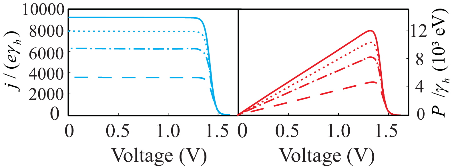
Figure 3: (Color online) Fig. 3 (a)-(d) show the time evolution of the population on each level of two-pathway model corresponding to Fig. 2 (b) at room temperature T=300​KT=300{\rm{K}}: ρb​b{\rho_{bb}} in red-dashed, ρa1​a1{\rho_{{a_{1}}{a_{1}}}} (ρa2​a2{\rho_{{a_{2}}{a_{2}}}}) in orange-dot-dashed, ρα1​α1{\rho_{{\alpha_{1}}{\alpha_{1}}}} (ρα2​α2{\rho_{{\alpha_{2}}{\alpha_{2}}}}) in green-solid, and ρβ1​β1{\rho_{{\beta_{1}}{\beta_{1}}}} (ρβ2​β2{\rho_{{\beta_{2}}{\beta_{2}}}}) in black-dotted line. The cross-coupling Γ12​c=ηc2​Γ1​c​Γ2​c{\Gamma_{12c}}={\eta_{{c_{2}}}}\sqrt{{\Gamma_{1c}}{\Gamma_{2c}}} takes ηc2=0,0.3,0.6,1{\eta_{{c_{2}}}}=0,0.3,0.6,1 for (a), (b), (c) and (d), respectively. The other cross-couplings γ12​h=ηh​γ1​h​γ2​h{\gamma_{12h}}={\eta_{h}}\sqrt{{\gamma_{1h}}{\gamma_{2h}}}, γk​l​m​n=ηc11​γk​l​γm​n{\gamma_{klmn}}=\eta_{{c_{1}}}^{1}\sqrt{{\gamma_{kl}}{\gamma_{mn}}} (k​l≠m​nkl\neq mn) and γk​l​m​n=ηc12​γk​l​γm​n{\gamma_{klmn}}=\eta_{{c_{1}}}^{2}\sqrt{{\gamma_{kl}}{\gamma_{mn}}} (k​l≠m​nkl\neq mn) take the maximal values, i.e., ηh=ηc11=ηc12=1{\eta_{h}}=\eta_{{c_{1}}}^{1}=\eta_{{c_{1}}}^{2}=1. (e) and (f) are plotted for the current and power generated as a function of effective voltage VV at room temperature: ηc2=0{\eta_{{c_{2}}}}=0 in solid, ηc2=0.3{\eta_{{c_{2}}}}=0.3 in dotted, ηc2=0.6{\eta_{{c_{2}}}}=0.6 in dot-dashed and ηc2=0.9{\eta_{{c_{2}}}}=0.9 in dashed line.

Interestingly, the j−Vj-V and P−VP-V behaviors demonstrate that as cross-coupling strength Γ12​c{\Gamma_{12c}} increases, the current and power decrease, see Fig. 3 (e) and (f). This is different from the results in previous works [23, 34]. Note that, the parameters chosen for the two pathways are the same (see, Table I{\rm I}), thus the population on |a1⟩\left|{{a_{1}}}\right\rangle and |a2⟩\left|{{a_{2}}}\right\rangle is the same, so is the population on |α1⟩\left|{{\alpha_{1}}}\right\rangle and |α2⟩\left|{{\alpha_{2}}}\right\rangle, |β1⟩\left|{{\beta_{1}}}\right\rangle and |β2⟩\left|{{\beta_{2}}}\right\rangle. From Fig. 3 (d), we see that, the maximal Γ12​c{\Gamma_{12c}} (ηc2=1{\eta_{{c_{2}}}}=1) benefits the population on |β1⟩\left|{{\beta_{1}}}\right\rangle and |β2⟩\left|{{\beta_{2}}}\right\rangle and leads this population dominant over the others. Therefore we cannot plot j−Vj-V characteristics in this case as ρα1​α1=ρα2​α2=0{\rho_{{\alpha_{1}}{\alpha_{1}}}}={\rho_{{\alpha_{2}}{\alpha_{2}}}}=0. It was shown in Ref. [23, 34] that the power is increased and the current-voltage characteristic of the heat engine gets better with Fano interference. Here Fano interference characterized by Γ12​c{\Gamma_{12c}}, however, shows an opposite effect. We will explain this observation in subsection D. So, in the following numerical simulations, we will take Γ12​c=0{\Gamma_{12c}}=0.

III.2 Cross-couplings induced by LTR1

Fig. 4 shows that, current and power are enhanced as γ11,21{\gamma_{11,21}} and γ12,22{\gamma_{12,22}} increase, which coincides with the results predicted by Dorfman e​tet a​lal. This gives rise to a question that why does Γ12​c{\Gamma_{12c}} exhibit effects different from that by γ11,21{\gamma_{11,21}} and γ12,22{\gamma_{12,22}}?

Refer to caption
Figure 4: (Color online) Fig. 4 (a) - (d) show the time evolution of the population on each level in the two-pathway model shown in Fig. 2 (b) at room temperature T=300​KT=300{\rm{K}}. ρb​b{\rho_{bb}} was plotted in red-dashed, ρa1​a1{\rho_{{a_{1}}{a_{1}}}} (ρa2​a2{\rho_{{a_{2}}{a_{2}}}}) in orange-dot-dashed, ρα1​α1{\rho_{{\alpha_{1}}{\alpha_{1}}}} (ρα2​α2{\rho_{{\alpha_{2}}{\alpha_{2}}}}) in green-solid, and ρβ1​β1{\rho_{{\beta_{1}}{\beta_{1}}}} (ρβ2​β2{\rho_{{\beta_{2}}{\beta_{2}}}}) in black-dotted line. ηc11\eta_{{c_{1}}}^{1} in the cross-couplings γk​l​m​n=ηc11​γk​l​γm​n{\gamma_{klmn}}=\eta_{{c_{1}}}^{1}\sqrt{{\gamma_{kl}}{\gamma_{mn}}} (k​l≠m​nkl\neq mn) takes ηc11=0,0.3,0.6,1\eta_{{c_{1}}}^{1}=0,0.3,0.6,1 for (a), (b), (c) and (d), respectively. The other cross-couplings γ12​h=ηh​γ1​h​γ2​h{\gamma_{12h}}=\eta_{{h}}\sqrt{{\gamma_{1h}}{\gamma_{2h}}} and γk​l​m​n=ηc12​γk​l​γm​n{\gamma_{klmn}}=\eta_{{c_{1}}}^{2}\sqrt{{\gamma_{kl}}{\gamma_{mn}}} (k​l≠m​nkl\neq mn) take the maximal values, i.e., ηh=ηc12=1{\eta_{h}}=\eta_{{c_{1}}}^{2}=1. As mentioned in the last subsection, Γ12​c=0{\Gamma_{12c}}=0. (e) and (f) are plotted for the current and power generated as a function of effective voltage VV at room temperature. Dashed line is for ηc11=0\eta_{{c_{1}}}^{1}=0, dot-dashed for ηc11=0.3\eta_{{c_{1}}}^{1}=0.3, dotted line for ηc11=0.6\eta_{{c_{1}}}^{1}=0.6, and ηc11=1\eta_{{c_{1}}}^{1}=1 is ploted in thin-solid line.

Fig. 5 shows that, population in each state seems no difference for any values of the second type of cross-couplings γk​l​m​n=ηc12​γk​l​γm​n{\gamma_{klmn}}=\eta_{{c_{1}}}^{2}\sqrt{{\gamma_{kl}}{\gamma_{mn}}} (k​l≠m​nkl\neq mn). Thus different from couplings with γ1121{\gamma_{1121}} (γ1222{\gamma_{1222}}) and γ12​c{\gamma_{12c}}, the second type of cross-couplings has marginal effects on the current and power. This is analogous to quantum beats, which can occur in a VV type atom, but can not in a Λ\Lambda type atom based on the theory of quantum electrodynamics (QED)[38], as shown in Fig. 6.

Refer to caption
Figure 5: (Color online) Fig. 5 (a)-(d) show the time evolution of the population on each level of the system depicted in Fig. 2 (b) at room temperature T=300​KT=300{\rm{K}}: ρb​b{\rho_{bb}} in red-dashed, ρa1​a1{\rho_{{a_{1}}{a_{1}}}} (ρa2​a2{\rho_{{a_{2}}{a_{2}}}}) in orange-dot-dashed, ρα1​α1{\rho_{{\alpha_{1}}{\alpha_{1}}}} (ρα2​α2{\rho_{{\alpha_{2}}{\alpha_{2}}}}) in green-solid, and ρβ1​β1{\rho_{{\beta_{1}}{\beta_{1}}}} (ρβ2​β2{\rho_{{\beta_{2}}{\beta_{2}}}}) in black-dotted line. The cross-couplings γk​l​m​n=ηc12​γk​l​γm​n{\gamma_{klmn}}=\eta_{{c_{1}}}^{2}\sqrt{{\gamma_{kl}}{\gamma_{mn}}} (k​l≠m​nkl\neq mn) take ηc12=0,0.3,0.6,1\eta_{{c_{1}}}^{2}=0,0.3,0.6,1 for (a), (b), (c) and (d), respectively. The other cross-couplings γ12​h=ηh​γ1​h​γ2​h{\gamma_{12h}}=\eta_{h}\sqrt{{\gamma_{1h}}{\gamma_{2h}}} and γk​l​m​n=ηc11​γk​l​γm​n{\gamma_{klmn}}=\eta_{{c_{1}}}^{1}\sqrt{{\gamma_{kl}}{\gamma_{mn}}} (k​l≠m​nkl\neq mn) take the maximal values, i.e., ηh=ηc11=1{\eta_{h}}=\eta_{{c_{1}}}^{1}=1. Γ12​c=0{\Gamma_{12c}}=0. (e) and (f) are plotted for the current and power as a function of effective voltage VV at room temperature T=300​KT=300{\rm{K}}. Actually, we plot four curves in (e) and (f) with ηc12=0,0.3,0.6,1\eta_{{c_{1}}}^{2}=0,0.3,0.6,1, respectively, although all them overlap. Since (a)-(d) do not show any difference for different ηc12\eta_{{c_{1}}}^{2}, the j−Vj-V and P−VP-V behaviors are exactly the same for different ηc12\eta_{{c_{1}}}^{2}.
Refer to caption
Figure 6: (Color online) Three-level atomic structures for (a) VV-type and (b) Λ\Lambda-type quantum beat.

VV-type atom in excited states decays via the emission of a photon with frequency ν1{\nu_{1}} or ν2{\nu_{2}}. Since both emissions lead to the same final state, we cannot determine along w​h​i​c​hwhich p​a​t​hpath, ν1{\nu_{1}} or ν2{\nu_{2}}, the atom decays. This uncertainty leads to an interference between ν1{\nu_{1}} and ν2{\nu_{2}}, exhibiting quantum beats. A Λ\Lambda-type atom also decays via the emission of a photon with frequency ν1{\nu_{1}} or ν2{\nu_{2}}. However, an observation of atom at a long time after the emission can tell us which channel (1 or 2) was taken (atom in |b1⟩\left|{{b_{1}}}\right\rangle or |b2⟩\left|{{b_{2}}}\right\rangle). Consequently, we expect no beats in this case. For the model of Fig. 2 (b), transitions described by the second type of cross-couplings lead to different lower states, which do not induce interference. Thus the second type of cross-couplings has no effect on the j−Vj-V and P−VP-V behaviors.

With this consideration, in the following numerical simulations, we take γk​l​m​n=ηc12​γk​l​γm​n=0{\gamma_{klmn}}=\eta_{{c_{1}}}^{2}\sqrt{{\gamma_{kl}}{\gamma_{mn}}}=0.

III.3 Cross-couplings induced by HTR

As expected, γ12​h{\gamma_{12h}} benefits the transition as seen from Fig. 7. Inspired by the physics behind the quantum beat, we claim that interference can play an important role in the current and power only when the upper two levels |a1⟩\left|{{a_{1}}}\right\rangle and |a2⟩\left|{{a_{2}}}\right\rangle are coherently excited at the initial time. When the coherence between |a1⟩\left|{{a_{1}}}\right\rangle and |a2⟩\left|{{a_{2}}}\right\rangle is absent, i.e., seting γ12​h=0{\gamma_{12h}}=0, γ12​c{\gamma_{12c}} itself may suppress the exciton transfer. Equivalently, setting γ12​c=0{\gamma_{12c}}=0, γ12​h{\gamma_{12h}} itself may inhibit the current and power. In terms of steady-state solution to Eq. 1, we further confirm this observation, and it shows how these two types of interference work together to affect the transitions.

Refer to caption
Figure 7: (Color online) Fig. 7 (a)-(d) show the time evolution of the population on each level of the system in Fig. 2 (b) at room temperature T=300​KT=300{\rm{K}}. ρb​b{\rho_{bb}} is shown in red-dashed, ρa1​a1{\rho_{{a_{1}}{a_{1}}}} (ρa2​a2{\rho_{{a_{2}}{a_{2}}}}) in orange-dot-dashed, ρα1​α1{\rho_{{\alpha_{1}}{\alpha_{1}}}} (ρα2​α2{\rho_{{\alpha_{2}}{\alpha_{2}}}}) in green-solid, and ρβ1​β1{\rho_{{\beta_{1}}{\beta_{1}}}} (ρβ2​β2{\rho_{{\beta_{2}}{\beta_{2}}}}) in black-dotted line. The cross-couplings γ12​h=ηh​γ1​h​γ2​h{\gamma_{12h}}=\eta_{h}\sqrt{{\gamma_{1h}}{\gamma_{2h}}} take ηh=0,0.3,0.6,1\eta_{h}=0,0.3,0.6,1 for (a), (b), (c) and (d), respectively. The other cross-couplings γk​l​m​n=ηc11​γk​l​γm​n{\gamma_{klmn}}=\eta_{{c_{1}}}^{1}\sqrt{{\gamma_{kl}}{\gamma_{mn}}} (k​l≠m​nkl\neq mn) takes the maximal value, i.e., ηc11=1\eta_{{c_{1}}}^{1}=1. γk​l​m​n=ηc12​γk​l​γm​n=0{\gamma_{klmn}}=\eta_{{c_{1}}}^{2}\sqrt{{\gamma_{kl}}{\gamma_{mn}}}=0 (k​l≠m​nkl\neq mn) and Γ12​c=0{\Gamma_{12c}}=0. (e) and (f) are plotted for the current and power as a function of effective voltage VV at room temperature. ηh=0\eta_{h}=0 is plotted in dashed, ηh=0.3\eta_{h}=0.3 in dot-dashed, ηh=0.6\eta_{h}=0.6 in dotted and ηh=1\eta_{h}=1 in thin-solid line.

III.4 Combined effects of HTR and LTR1

For simplicity, we plot the steady-state j−Vj-V characteristic and power for one-pathway model in Fig. 8. We set γ12​c=ηc1′​γ1​c​γ2​c{\gamma_{12c}}={\eta^{\prime}_{{c_{1}}}}\sqrt{{\gamma_{1c}}{\gamma_{2c}}} and γ12​h=ηh​γ1​h​γ2​h{\gamma_{12h}}={\eta_{h}}\sqrt{{\gamma_{1h}}{\gamma_{2h}}}, thus ηc1′=1{\eta^{\prime}_{{c_{1}}}}=1 (ηh=1{\eta_{h}}=1) corresponds to the maximal coherence and ηc1′=0{\eta^{\prime}_{{c_{1}}}}=0 (ηh=0{\eta_{h}}=0) the minimal coherence.

Refer to caption
Figure 8: (Color online) Counter plot of the current as a function of cross-couplings γ12​c{\gamma_{12c}} and γ12​h{\gamma_{12h}}. As γ12​c=η′c1​γ1​c​γ2​c{\gamma_{12c}}={{\eta^{\prime}}_{{c_{1}}}}\sqrt{{\gamma_{1c}}{\gamma_{2c}}} (γ12​h=ηh​γ1​h​γ2​h)({\gamma_{12h}}={\eta_{h}}\sqrt{{\gamma_{1h}}{\gamma_{2h}}}), η′c1=1{{\eta^{\prime}}_{{c_{1}}}}=1 (ηh=1){\rm{({\eta_{h}}=1)}} corresponds to the maximal coherence and η′c1=0{{\eta^{\prime}}_{{c_{1}}}}=0 (ηh=0){\rm{({\eta_{h}}=0)}} the minimal coherence.

We observe that, when γ12​h{\gamma_{12h}} is very small, the current and power decrease with the increasing of γ12​c{\gamma_{12c}}. Similarly, when γ12​c{\gamma_{12c}} is very small, large γ12​h{\gamma_{12h}} inhibits the transitions. Recall the quantum beats, if one of γ12​h{\gamma_{12h}} and γ12​c{\gamma_{12c}} is very small, |a1⟩\left|{{a_{1}}}\right\rangle and |a2⟩\left|{{a_{2}}}\right\rangle are almost independently excited. For this reason, when one cross-coupling term becomes very large, the current and power will be suppressed. When both γ12​h{\gamma_{12h}} and γ12​c{\gamma_{12c}} increase to a certain value, strong cross-couplings can enhance the current and power. This conclusion holds for γ1121{\gamma_{1121}} and γ1222{\gamma_{1222}} in the two-pathway model. For the terms with Γ12​c{\Gamma_{12c}} discussed in subsection A, |β1⟩\left|{{\beta_{1}}}\right\rangle and |β2⟩\left|{{\beta_{2}}}\right\rangle obviously, are not in a coherent state. As a result, the transition process is suppressed as Γ12​c{\Gamma_{12c}} increases.

IV Effect of Multiple pathways

Electron transfer in the PSII RC has been thoroughly studied and several charge-separation pathways were identified. In this section, we investigate the role of multiple pathways on the behavior of j−Vj-V and P−VP-V. The simulation results are presented in Fig. 9. From Fig. 9 we find that as the number of pathways increases, the BQHE produces stronger current and power. Especially, the model of two pathways, corresponding to Fig. 2 (b), shows a current enhancement of 76.8%76.8\%, comparing with the case of only one pathway shown in Fig. 2 (a). Nevertheless, with the number of pathways increase further, the enhancement rate decreases. The current of three-pathway model shows 25.9%25.9\% more than that of two-pathway model, and the current of four-pathway model just 16.7%16.7\% more than that of three-pathway one.

Refer to caption
Figure 9: (Color online) The current and power as a function of effective voltage VV at room temperature for different numbers of pathway. The results for one pathway are shown in dashed, two pathways in dot-dashed, three in dotted, four in thin-solid line. Cross-couplings corresponding to LTR2 and the second type of cross-couplings corresponding to LTR1 are set to 00. All the other cross-couplings take their maximal values.

The observations can be understood as follows: the current and power of the BQHE sharply depends on the rate of transition from the ground state |b⟩\left|b\right\rangle to state |a1⟩\left|{{a_{1}}}\right\rangle or |a2⟩\left|{{a_{2}}}\right\rangle, i.e., the decay rate in HTR. More pathways mathematically equal to increasing the strength of the decay rate in LTR1 and LTR2. When γ1​h{\gamma_{1h}}, γ2​h{\gamma_{2h}} and γ12​h{\gamma_{12h}} take a fixed value, the energy flux density is fixed. The strength of the decay rate in LTR1 and LTR2, or rather the number of pathways should match the transport rate in HTR, otherwise, excessive pathways can not significantly improve the transition process. We further propose that in order to accelerate the transfer process, multiple pathways in the BQHE (or similar structure in the natural photosynthetic reaction center) are a better choice comparing with simply increasing the strength of the decay rates and cross-couplings related to LTR1 and LTR2 within one-pathway model. As shown in Appendix, the decay rates or cross-couplings are given by γk​l​m​n=2​p2​Vp​h​n​gk​l​p​gm​n​pπ​c{\gamma_{klmn}}=\frac{{2{p^{2}}{V_{phn}}{g_{klp}}{g_{mnp}}}}{{\pi c}}, from which we know that these rates are determined by the ambient phonon reservoir and the diploe moment of |a1,2⟩↔|b⟩\left|{{a_{1,2}}}\right\rangle\leftrightarrow\left|b\right\rangle for LTR1 (|β1,2⟩↔|b⟩\left|{{\beta_{1,2}}}\right\rangle\leftrightarrow\left|b\right\rangle for LTR2). The natural condition of reservoir is hot and wet, and generally unstable. And the structure of RC complexes is born fixed, resulting in constant diploe moment between different states of pigment molecules. Therefore, these factors cannot be utilized to enhance the reaction efficiency. Nevertheless, more charge-separation pathways means increasing reaction channels. This seems easy to achieve. In the next section, considering acceptor-to-donor charge recombination and noise-induced dephasing, we will show that multiple pathways is still a better choice in contrast with increasing the strength of the decay rate in LTR1 and LTR2.

Refer to caption
Figure 10: (Color online) (a) is plotted for the current ratio defined by (j⁡(χ=0)−j⁡(χ))/j⁡(χ=0)({j(\chi=0)-j(\chi)})/{j(\chi=0)} as a function of the recombination rate for one- and two-pathway models. The blue-solid and red-dashed lines are for the maximal coherence, i.e., all the cross-couplings take the maximal values, except that cross-couplings induced by LTR2 and the second type of cross-couplings induced by LTR1 are set to 00. The blue-dot-dashed and red-dotted lines are for the minimal coherence, i.e., all the cross-couplings take the minimal values 0. The blue lines stand for one-pathway model with the strength of the decay rates in LTR1 and LTR2 and the relaxation rate doubled and the other parameters fixed. The red lines stand for two-pathway one. (b) is the case of one- and three-pathway models. The blue-solid and red-dashed lines are for the maximal coherence while the blue-dot-dashed and red-dotted lines are for the minimal coherence. The blue lines stand for one-pathway model with the strength of the decay rates in LTR1 and LTR2 and the relaxation rate tripled and the other parameters fixed. The red lines stand for three-pathway one.

V Effects of recombination and dephasing

In this section, we examine how charge recombination at the acceptor/donor interface and dephasing of |a1⟩\left|{{a_{1}}}\right\rangle and |a2⟩\left|{{a_{2}}}\right\rangle affects the current and power. In Fig. 10 (a), we plot the relative change of current as a function of the recombination rate χ\chi. The relative change of current is defined by (j⁡(χ=0)−j⁡(χ))​/​j​(χ=0){{\left({j(\chi=0)-j(\chi)}\right)}\mathord{\left/{\vphantom{{\left({j(\chi=0)-j(\chi)}\right)}{j(\chi=0)}}}\right.\kern-1.2pt}{j(\chi=0)}}. We calculate this relative change for both cases of maximal coherence and minimal coherence with one and two pathways, respectively. To determine which one, multiple pathways or large decay rates in LTR1 and LTR2, is a better choice, we double these decay rates and the relaxation rate in one-pathway model with the other parameters fixed. Fig. 10 (b) shows the relative current change for both cases of maximal coherence and minimal coherence with one and three pathways, respectively. Similarly, we triple these decay rates and the relaxation rate in one-pathway model with the other parameters fixed. Fig. 10 (a) and Fig. 10 (b) show that as the recombination rate increases, the current decreases monotonically as expected. Nevertheless, the set-up with maximal coherence can better reduce the impact of acceptor-to-donor charge recombination. Therefore, noise-induced coherence between |a1⟩\left|{{a_{1}}}\right\rangle and |a2⟩\left|{{a_{2}}}\right\rangle due to Fano interference can diminish the influence of recombination. Besides, we observe that the larger number of the pathways is, the more robust the system against the recombination. Therefore, in the presence of the additional loss mechanism due to acceptor-to-donor charge recombination, the maximal coherence scheme/multi-pathway set-up is more efficient than the minimal coherence scheme/one-pathway one.

Next we explore whether, in the presence of dephasing, the multi-pathway set-up can still benefit the current and power. We calculate the relative change of current as a function of the dephasing rate Γd​e​p{\Gamma_{dep}} and present the results in Fig. 11. The relative change of current has also been calculated for different numbers of pathways. Similarly, to compare the two choices of multiple pathways and increasing the strength of the decay rate in LTR1 and LTR2, we modify these decay rates and the relaxation rate in one-pathway model with the other parameters fixed, just as in the case of the relaxation rate discussed above. Observing the results, we find that the current decreases monotonically as the dephasing rate increases. Besides, the more pathways, the more robust against the dephasing. Therefore, the multiple-pathway model is more efficient than the one-pathway one even in the presence of depasing process mechanism.

Refer to caption
Figure 11: (Color online) (a) is the relative current change (defined by (j⁡(Γd​e​p=0)−j⁡(Γd​e​p))/j⁡(Γd​e​p=0)(j({\Gamma_{dep}}=0)-j({\Gamma_{dep}}))/j({\Gamma_{dep}}=0)) as a function of dephasing rate. The blue-dashed line is for one-pathway model with the strength of the decay rates in LTR1 and LTR2 and the relaxation rate doubled and the other parameters fixed. The red-solid line is for two-pathway one. (b) is the case of one- and three-pathway model. The blue-dashed line is for one-pathway model with the strength of the decay rates in LTR1 and LTR2 and the relaxation rate tripled and the other parameters fixed. The red-solid line is for three-pathway one. The dimensionless parameter χ=0.2\chi=0.2 as in Table I{\rm I}.

VI Conclusion

In conclusion, we have studied the dynamics of two-pathway biological quantum heat engine and calculated the steady-state current-voltage (j−Vj-V) and power-voltage (P−VP-V) characteristics. We explored the effect of various cross-couplings, and found that only the cross-couplings describing transitions between high levels and the same lower energy level have effects on the j−Vj-V and P−VP-V behaviors. We explained the physics behind this observation using the concept of quantum beat. Furthermore we find that the current and power can be increased due to Fano interference when the upper two levels are in a coherent supposition. Finally, we calculate the j−Vj-V and P−VP-V characteristics subjected to acceptor-to-donor charge recombination and dephasing, and show that noise-induced quantum coherence helps in the suppression of the influence of the acceptor-to-donor charge recombination. These results suggest that multi-pathway BQHE can benefit the charge separation and the light-harvesting yields, and it is a better choice in contrast with increasing the strength of decay rates and cross-couplings.

VII acknowledgments

This work is supported by National Natural Science Foundation of China (NSFC) under Grants No. 11175032, and No. 61475033.

Appendix A The derivation of Eq. (1)

In this part, we will present a derivation for the master equation used in the maintext. We consider a total Hamiltonian

H^=H^S+H^R+H^S​R,\displaystyle\begin{aligned} \hat{H}={{\hat{H}}_{S}}+{{\hat{H}}_{R}}+{{\hat{H}}_{SR}},\end{aligned} (9)

where the system Hamiltonian

H^S=ℏωb|b⟩⟨b|+ℏωa1|a1⟩⟨a1|+ℏωa2|a2⟩⟨a2|,\displaystyle\begin{aligned} {{\hat{H}}_{S}}=\hbar{\omega_{b}}\left|b\right\rangle\left\langle b\right|+\hbar{\omega_{{a_{1}}}}\left|{{a_{1}}}\right\rangle\left\langle{{a_{1}}}\right|+\hbar{\omega_{{a_{2}}}}\left|{{a_{2}}}\right\rangle\left\langle{{a_{2}}}\right|,\end{aligned} (10)

with ℏ​ωai,b=Eai,b\hbar{\omega_{{a_{i}},b}}={E_{{a_{i}},b}} (i=1,2)(i=1,2) being the energy of states |ai⟩\left|{{a_{i}}}\right\rangle, |b⟩\left|b\right\rangle.

H^R{{\hat{H}}_{R}} represents the Hamiltonian of the high temperature photon reservoir (HTR)

H^R=∑pℏ​νp​b^p†​b^p.\displaystyle\begin{aligned} {{\hat{H}}_{R}}=\sum\limits_{p}{\hbar{\nu_{p}}\hat{b}_{p}^{\dagger}{{\hat{b}}_{p}}}.\end{aligned} (11)

Here b^p†{\hat{b}_{p}^{\dagger}} and b^p{{{\hat{b}}_{p}}} denote the creation and destruction operators. The interaction Hamiltonian in the rotating-wave approximation (RWA) is

H^S​R=ℏ​∑pg1​p​σ^h​1​b^p†+ℏ​∑qg2​q​σ^h​2​b^q†+H.c.,\displaystyle\begin{aligned} {{\hat{H}}_{SR}}=\hbar\sum\limits_{p}{{g_{1p}}{{\hat{\sigma}}_{h1}}\hat{b}_{p}^{\dagger}}+\hbar\sum\limits_{q}{{g_{2q}}{{\hat{\sigma}}_{h2}}{\hat{b}_{q}^{\dagger}}}+{\rm{H}}{\rm{.c}}{\rm{.}},\end{aligned} (12)

with σ^h​1=|b⟩⟨a1|{{\hat{\sigma}}_{h1}}=\left|b\right\rangle\langle{a_{1}}| and σ^h​2=|b⟩⟨a2|{{\hat{\sigma}}_{h2}}=\left|b\right\rangle\langle{a_{2}}| being the lower operators. The coupling constant g1​p=−℘a1​b⋅ϵ^p​ℰpℏg_{1p}=-\frac{{{\wp_{{a_{1}}b}}}\cdot\hat{\epsilonup}_{p}\mathscr{E}_{p}}{\hbar} and g2​q=−℘a2​b⋅ϵ^q​ℰpℏg_{2q}=-\frac{{{\wp_{{a_{2}}b}}}\cdot\hat{\epsilonup}_{q}\mathscr{E}_{p}}{\hbar}, where ℘a1​b{{\wp_{{a_{1}}b}}} (℘a2​b{{\wp_{{a_{2}}b}}}) is the dipole moment of |a1⟩↔|b⟩\left|{{a_{1}}}\right\rangle\leftrightarrow\left|b\right\rangle (|a2⟩↔|b⟩\left|{{a_{2}}}\right\rangle\leftrightarrow\left|b\right\rangle ). ϵ^p\hat{\epsilonup}_{p} (ϵ^q\hat{\epsilonup}_{q}) is the polarization of the field. The electric field per photon is ℰp,q=(ℏ​νp,q2​ϵ0​V)12\mathscr{E}_{p,q}=(\frac{\hbar{\nu_{p,q}}}{2{\epsilonup}_{0}V})^{\frac{1}{2}}.

It is convenient to work in the interaction picture. The Hamiltonian, in the interaction picture, is given by

V^​(t)=ℏ​∑kg1​p​b^p†​σ^h​1​e−i⁡(ωa1​b−νp)​t+ℏ∑qg2​qb^q†σ^h​2e−i⁡(ωa2​b−νq)​t+H.c..\displaystyle\begin{aligned} \hat{V}(t)=&\hbar\sum\limits_{k}{{g_{1p}}\hat{b}_{p}^{\dagger}{{\hat{\sigma}}_{h1}}{e^{-i({\omega_{{a_{1}}b}}-{\nu_{p}})t}}}\\ &+\hbar\sum\limits_{q}{{g_{2q}}\hat{b}_{q}^{\dagger}{{\hat{\sigma}}_{h2}}{e^{-i({\omega_{{a_{2}}b}}-{\nu_{q}})t}}}+{\rm{H}}{\rm{.c}}{\rm{.}}.\end{aligned} (13)

The equation of motion for the system density operator ρ^S{\hat{\rho}_{S}} is

d​ρ^S​(t)d​t=−iℏ​TrR​[V^​(t),ρ^S​(0)⊗ρ^R​(0)]−1ℏ2TrR∫0t[V^(t),[V^(t′),ρ^S(t′)⊗ρ^R(0)]]dt′.\displaystyle\begin{aligned} \frac{{d{{\hat{\rho}}_{S}}(t)}}{{dt}}=&-\frac{i}{\hbar}{\rm{T}}{{\rm{r}}_{R}}[\hat{V}(t),{{\hat{\rho}}_{S}}(0)\otimes{{\hat{\rho}}_{R}}(0)]\\ &-\frac{1}{{{\hbar^{2}}}}{\rm{T}}{{\rm{r}}_{R}}\int_{0}^{t}{[\hat{V}(t),[\hat{V}(t^{\prime}),{{\hat{\rho}}_{S}}(t^{\prime})\otimes{{\hat{\rho}}_{R}}(0)]]dt^{\prime}}.\end{aligned} (14)

Substituting V^​(t)\hat{V}(t) into Eq. (14), we have,

d​ρ^S​(t)d​t=−∫0tdt′{∑p,p′g1​pg1​p′ei⁡(ωa1​b−νp)​t−i⁡(ωa1​b−νp′)​t′TrR[σ^h​1+b^p,[b^p′†σ^h​1,ρ^S(t′)⊗ρ^R(0)]]+∑p,q′g1​pg2​q′ei⁡(ωa1​b−νp)​t−i⁡(ωa2​b−νq′)​t′TrR[σ^h​1+b^p,[b^q′†σ^h​2,ρ^S(t′)⊗ρ^R(0)]]+∑q,p′g2​qg1​p′ei⁡(ωa2​b−νq)​t−i⁡(ωa1​b−νp′)​t′TrR[σ^h​2+b^q,[b^p′†σ^h​1,ρ^S(t′)⊗ρ^R(0)]]+∑q,q′g2​qg2​q′ei⁡(ωa2​b−νq)​t−i⁡(ωa2​b−νq′)​t′TrR[σ^h​2+b^q,[b^q′†σ^h​2,ρ^S(t′)⊗ρ^R(0)]]+∑p,p′g1​pg1​p′e−i⁡(ωa1​b−νp)​t+i⁡(ωa1​b−νp′)​t′TrR[b^p†σ^h​1,[σ^h​1+b^p′,ρ^S(t′)⊗ρ^R(0)]]+∑p,q′g1​pg2​q′e−i⁡(ωa1​b−νp)​t+i⁡(ωa2​b−νq′)​t′TrR[b^p†σ^h​1,[σ^h​2+b^q′,ρ^S(t′)⊗ρ^R(0)]]+∑q,p′g2​qg1​p′e−i⁡(ωa2​b−νq)​t+i⁡(ωa1​b−νp′)​t′TrR[b^q†σ^h​2,[σ^h​1+b^p′,ρ^S(t′)⊗ρ^R(0)]]+∑q,q′g2​qg2​q′e−i⁡(ωa2​b−νq)​t+i⁡(ωa2​b−νq′)​t′TrR[b^q†σ^h​2,[σ^h​2+b^q′,ρ^S(t′)⊗ρ^R(0)]]}.\displaystyle\begin{aligned} \frac{{d{{\hat{\rho}}_{S}}(t)}}{{dt}}=&-\int_{0}^{t}{dt^{\prime}}\left\{{\sum\limits_{p,p^{\prime}}{{g_{1p}}{g_{1p^{\prime}}}}}\right.{e^{i({\omega_{{a_{1}}b}}-{\nu_{p}})t-i({\omega_{{a_{1}}b}}-{\nu_{p^{\prime}}})t^{\prime}}}{\rm{T}}{{\rm{r}}_{R}}\left[{\hat{\sigma}_{h1}^{+}{{\hat{b}}_{p}},\left[{\hat{b}_{p^{\prime}}^{\dagger}{{\hat{\sigma}}_{h1}},{{\hat{\rho}}_{S}}(t^{\prime})\otimes{{\hat{\rho}}_{R}}(0)}\right]}\right]\\ &+\sum\limits_{p,q^{\prime}}{{g_{1p}}{g_{2q^{\prime}}}{e^{i({\omega_{{a_{1}}b}}-{\nu_{p}})t-i({\omega_{{a_{2}}b}}-{\nu_{q^{\prime}}})t^{\prime}}}}{\rm{T}}{{\rm{r}}_{R}}\left[{\hat{\sigma}_{h1}^{+}{{\hat{b}}_{p}},\left[{\hat{b}_{q^{\prime}}^{\dagger}{{\hat{\sigma}}_{h2}},{{\hat{\rho}}_{S}}(t^{\prime})\otimes{{\hat{\rho}}_{R}}(0)}\right]}\right]\\ &+\sum\limits_{q,p^{\prime}}{{g_{2q}}{g_{1p^{\prime}}}{e^{i({\omega_{{a_{2}}b}}-{\nu_{q}})t-i({\omega_{{a_{1}}b}}-{\nu_{p^{\prime}}})t^{\prime}}}}{\rm{T}}{{\rm{r}}_{R}}\left[{\hat{\sigma}_{h2}^{+}{{\hat{b}}_{q}},\left[{\hat{b}_{p^{\prime}}^{\dagger}{{\hat{\sigma}}_{h1}},{{\hat{\rho}}_{S}}(t^{\prime})\otimes{{\hat{\rho}}_{R}}(0)}\right]}\right]\\ &+\sum\limits_{q,q^{\prime}}{{g_{2q}}{g_{2q^{\prime}}}{e^{i({\omega_{{a_{2}}b}}-{\nu_{q}})t-i({\omega_{{a_{2}}b}}-{\nu_{q^{\prime}}})t^{\prime}}}}{\rm{T}}{{\rm{r}}_{R}}\left[{\hat{\sigma}_{h2}^{+}{{\hat{b}}_{q}},\left[{\hat{b}_{q^{\prime}}^{\dagger}{{\hat{\sigma}}_{h2}},{{\hat{\rho}}_{S}}(t^{\prime})\otimes{{\hat{\rho}}_{R}}(0)}\right]}\right]\\ &+\sum\limits_{p,p^{\prime}}{{g_{1p}}{g_{1p^{\prime}}}{e^{-i({\omega_{{a_{1}}b}}-{\nu_{p}})t+i({\omega_{{a_{1}}b}}-{\nu_{p^{\prime}}})t^{\prime}}}}{\rm{T}}{{\rm{r}}_{R}}\left[{\hat{b}_{p}^{\dagger}{{\hat{\sigma}}_{h1}},\left[{\hat{\sigma}_{h1}^{+}{{\hat{b}}_{p^{\prime}}},{{\hat{\rho}}_{S}}(t^{\prime})\otimes{{\hat{\rho}}_{R}}(0)}\right]}\right]\\ &+\sum\limits_{p,q^{\prime}}{{g_{1p}}{g_{2q^{\prime}}}{e^{-i({\omega_{{a_{1}}b}}-{\nu_{p}})t+i({\omega_{{a_{2}}b}}-{\nu_{q^{\prime}}})t^{\prime}}}}{\rm{T}}{{\rm{r}}_{R}}\left[{\hat{b}_{p}^{\dagger}{{\hat{\sigma}}_{h1}},\left[{\hat{\sigma}_{h2}^{+}{{\hat{b}}_{q^{\prime}}},{{\hat{\rho}}_{S}}(t^{\prime})\otimes{{\hat{\rho}}_{R}}(0)}\right]}\right]\\ &+\sum\limits_{q,p^{\prime}}{{g_{2q}}{g_{1p^{\prime}}}{e^{-i({\omega_{{a_{2}}b}}-{\nu_{q}})t+i({\omega_{{a_{1}}b}}-{\nu_{p^{\prime}}})t^{\prime}}}}{\rm{T}}{{\rm{r}}_{R}}\left[{\hat{b}_{q}^{\dagger}{{\hat{\sigma}}_{h2}},\left[{\hat{\sigma}_{h1}^{+}{{\hat{b}}_{p^{\prime}}},{{\hat{\rho}}_{S}}(t^{\prime})\otimes{{\hat{\rho}}_{R}}(0)}\right]}\right]\\ &+\left.{\sum\limits_{q,q^{\prime}}{{g_{2q}}{g_{2q^{\prime}}}{e^{-i({\omega_{{a_{2}}b}}-{\nu_{q}})t+i({\omega_{{a_{2}}b}}-{\nu_{q^{\prime}}})t^{\prime}}}}{\rm{T}}{{\rm{r}}_{R}}\left[{\hat{b}_{q}^{\dagger}{{\hat{\sigma}}_{h2}},\left[{\hat{\sigma}_{h2}^{+}{{\hat{b}}_{q^{\prime}}},{{\hat{\rho}}_{S}}(t^{\prime})\otimes{{\hat{\rho}}_{R}}(0)}\right]}\right]}\right\}.\end{aligned} (15)

The sum over pp may be replaced by an integral through

∑p→Vp​h​tπ2∫0∞dpp2.\displaystyle\begin{aligned} \sum\limits_{p}{}\to\frac{{{V_{pht}}}}{{{\pi^{2}}}}\int_{0}^{\infty}{dp{p^{2}}}.\end{aligned} (16)

where Vp​h​t{{V_{pht}}} is the volume. Neglecting all memory effects and assuming that the density matrix is a slowly varying function of time, i.e., ρ^​(t′)≈ρ^​(t){\hat{\rho}}(t^{\prime})\approx{\hat{\rho}}(t), we obtain the integration over time as

∫0∞d​t′​ei⁡(ω−νk)​(t−t′)=π​δ​(ω−νk).\displaystyle\begin{aligned} \int_{0}^{\infty}{dt^{\prime}{e^{i(\omega-{\nu_{k}})(t-t^{\prime})}}}=\pi\delta(\omega-{\nu_{k}}).\end{aligned} (17)

Substitute (16) and (17) into (15) and note that ⟨b^p⟩=⟨b^p†⟩=0\left\langle{{{\hat{b}}_{p}}}\right\rangle=\left\langle{\hat{b}_{p}^{\dagger}}\right\rangle=0, ⟨b^p​b^p′⟩=⟨b^p†​b^p′†⟩=0\left\langle{{{\hat{b}}_{p}}{{\hat{b}}_{p^{\prime}}}}\right\rangle=\left\langle{\hat{b}_{p}^{\dagger}\hat{b}_{p^{\prime}}^{\dagger}}\right\rangle=0, ⟨b^p†​b^p′⟩=n¯p​δp​p′\left\langle{\hat{b}_{p}^{\dagger}{{\hat{b}}_{p^{\prime}}}}\right\rangle={{\bar{n}}_{p}}{\delta_{pp^{\prime}}}, and ⟨b^p​b^p′†⟩=(n¯p+1)​δp​p′\left\langle{{{\hat{b}}_{p}}\hat{b}_{p^{\prime}}^{\dagger}}\right\rangle=({{\bar{n}}_{p}}+1){\delta_{pp^{\prime}}}. The master equation reduces to

d​ρ^S​(t)d​t=Vp​h​tπ​c{p2g1​p2[(n¯p+1)(2σ^h​1ρ^S(t)σ^h​1†−σ^h​1†σ^h​1ρ^S(t)−ρ^S(t)σ^h​1†σ^h​1)]+p2​g1​p2​[n¯p​(2​σ^h​1†​ρ^S​(t)​σ^h​1−σ^h​1​σ^h​1†​ρ^S​(t)−ρ^S​(t)​σ^h​1​σ^h​1†)]+p2​g2​p2​[(n¯p+1)​(2​σ^h​2​ρ^S​(t)​σ^h​2†−σ^h​2†​σ^h​2​ρ^S​(t)−ρ^S​(t)​σ^h​2†​σ^h​2)]+p2​g2​p2​[n¯p​(2​σ^h​2†​ρ^S​(t)​σ^h​2−σ^h​2​σ^h​2†​ρ^S​(t)−ρ^S​(t)​σ^h​2​σ^h​2†)]+p2​g1​p​g2​p​[(n¯p+1)​(σ^h​1​ρ^S​(t)​σ^h​2†+σ^h​2​ρ^S​(t)​σ^h​1†)]+p2​g1​p​g2​p​[n¯p​(σ^h​1†​ρ^S​(t)​σ^h​2+σ^h​2†​ρ^S​(t)​σ^h​1)]+p2​g1​p​g2​p​[(n¯p+1)​(σ^h​2​ρ^S​(t)​σ^h​1†+σ^h​1​ρ^S​(t)​σ^h​2†)]+p2g1​pg2​p[n¯p(σ^h​2†ρ^S(t)σ^h​1+σ^h​1†ρ^S(t)σ^h​2)]}.\displaystyle\begin{aligned} \frac{{d{{\hat{\rho}}_{S}}(t)}}{{dt}}=&\frac{{{V_{pht}}}}{{\pi c}}\left\{{{p^{2}}g_{1p}^{2}\left[{\left({{{\bar{n}}_{p}}+1}\right)\left({2{{\hat{\sigma}}_{h1}}{{\hat{\rho}}_{S}}(t)\hat{\sigma}_{h1}^{\dagger}-\hat{\sigma}_{h1}^{\dagger}{{\hat{\sigma}}_{h1}}{{\hat{\rho}}_{S}}(t)-{{\hat{\rho}}_{S}}(t)\hat{\sigma}_{h1}^{\dagger}{{\hat{\sigma}}_{h1}}}\right)}\right]}\right.\\ &+{p^{2}}g_{1p}^{2}\left[{{{\bar{n}}_{p}}\left({2\hat{\sigma}_{h1}^{\dagger}{{\hat{\rho}}_{S}}(t){{\hat{\sigma}}_{h1}}-{{\hat{\sigma}}_{h1}}\hat{\sigma}_{h1}^{\dagger}{{\hat{\rho}}_{S}}(t)-{{\hat{\rho}}_{S}}(t){{\hat{\sigma}}_{h1}}\hat{\sigma}_{h1}^{\dagger}}\right)}\right]\\ &+{p^{2}}g_{2p}^{2}\left[{\left({{{\bar{n}}_{p}}+1}\right)\left({2{{\hat{\sigma}}_{h2}}{{\hat{\rho}}_{S}}(t)\hat{\sigma}_{h2}^{\dagger}-\hat{\sigma}_{h2}^{\dagger}{{\hat{\sigma}}_{h2}}{{\hat{\rho}}_{S}}(t)-{{\hat{\rho}}_{S}}(t)\hat{\sigma}_{h2}^{\dagger}{{\hat{\sigma}}_{h2}}}\right)}\right]\\ &+{p^{2}}g_{2p}^{2}\left[{{{\bar{n}}_{p}}\left({2\hat{\sigma}_{h2}^{\dagger}{{\hat{\rho}}_{S}}(t){{\hat{\sigma}}_{h2}}-{{\hat{\sigma}}_{h2}}\hat{\sigma}_{h2}^{\dagger}{{\hat{\rho}}_{S}}(t)-{{\hat{\rho}}_{S}}(t){{\hat{\sigma}}_{h2}}\hat{\sigma}_{h2}^{\dagger}}\right)}\right]\\ &+{p^{2}}{g_{1p}}{g_{2p}}\left[{\left({{{\bar{n}}_{p}}+1}\right)\left({{{\hat{\sigma}}_{h1}}{{\hat{\rho}}_{S}}(t)\hat{\sigma}_{h2}^{\dagger}+{{\hat{\sigma}}_{h2}}{{\hat{\rho}}_{S}}(t)\hat{\sigma}_{h1}^{\dagger}}\right)}\right]\\ &+{p^{2}}{g_{1p}}{g_{2p}}\left[{{{\bar{n}}_{p}}\left({\hat{\sigma}_{h1}^{\dagger}{{\hat{\rho}}_{S}}(t){{\hat{\sigma}}_{h2}}+\hat{\sigma}_{h2}^{\dagger}{{\hat{\rho}}_{S}}(t){{\hat{\sigma}}_{h1}}}\right)}\right]\\ &+{p^{2}}{g_{1p}}{g_{2p}}\left[{\left({{{\bar{n}}_{p}}+1}\right)\left({{{\hat{\sigma}}_{h2}}{{\hat{\rho}}_{S}}(t)\hat{\sigma}_{h1}^{\dagger}+{{\hat{\sigma}}_{h1}}{{\hat{\rho}}_{S}}(t)\hat{\sigma}_{h2}^{\dagger}}\right)}\right]\\ &+{p^{2}}{g_{1p}}{g_{2p}}\left.{\left[{{{\bar{n}}_{p}}\left({\hat{\sigma}_{h2}^{\dagger}{{\hat{\rho}}_{S}}(t){{\hat{\sigma}}_{h1}}+\hat{\sigma}_{h1}^{\dagger}{{\hat{\rho}}_{S}}(t){{\hat{\sigma}}_{h2}}}\right)}\right]}\right\}.\end{aligned} (18)

The indicator pp here is redefined as p=ωa1,2​bcp=\frac{{{\omega_{{a_{1,2}}b}}}}{c}. Introducing notations

γk​l​h=2​p2​Vp​h​t​gk​p​gl​pπ​c,\displaystyle\begin{aligned} {\gamma_{klh}}=\frac{{2{p^{2}}{V_{pht}}{g_{kp}}{g_{lp}}}}{{\pi c}},\end{aligned} (19)

where k,l=1,2k,l=1,2, gk,l​pg_{k,lp} is the coupling constant corresponding to transition with frequency ωa1,2​b\omega_{a_{1,2}b}, and the average occupation numbers of photons nh=n¯p{n_{h}}={\bar{n}}_{p}, we rewrite Eq. (18) in a simple form as

d​ρ^S​(t)d​t=∑k,l=1,2γk​l​h2[(nh+1)(σh​lρ^Sσh​k†+σh​kρ^Sσh​l†−σh​l†σh​kρ^S−ρ^Sσh​k†σh​l)+nh(σh​k†ρ^Sσh​l+σh​l†ρ^Sσh​k−σh​kσh​l†ρ^S−ρ^Sσh​lσh​k†)].\displaystyle\begin{aligned} \frac{{d{{\hat{\rho}}_{S}}(t)}}{{dt}}=&\sum\limits_{k,l=1,2}{\frac{{{\gamma_{klh}}}}{2}}[({n_{h}}+1)({\sigma_{hl}}{{\hat{\rho}}_{S}}\sigma_{hk}^{\dagger}+{\sigma_{hk}}{{\hat{\rho}}_{S}}\sigma_{hl}^{\dagger}-\sigma_{hl}^{\dagger}{\sigma_{hk}}{{\hat{\rho}}_{S}}-{{\hat{\rho}}_{S}}\sigma_{hk}^{\dagger}{\sigma_{hl}})\\ &+{n_{h}}(\sigma_{hk}^{\dagger}{{\hat{\rho}}_{S}}{\sigma_{hl}}+\sigma_{hl}^{\dagger}{{\hat{\rho}}_{S}}{\sigma_{hk}}-{\sigma_{hk}}\sigma_{hl}^{\dagger}{{\hat{\rho}}_{S}}-{{\hat{\rho}}_{S}}{\sigma_{hl}}\sigma_{hk}^{\dagger})].\end{aligned} (20)

The cross-couplings γk​l​h{{\gamma_{klh}}} for k≠lk\neq l corresponds to the strength of the Fano interference, and γk​k​h=γk​h{\gamma_{kkh}}={\gamma_{kh}} denotes the spontaneous decay rate. With this consideration, we finally obtain Eq. (3).

By the same procedure outlined for the transition |b⟩↔|a1,2⟩\left|b\right\rangle\leftrightarrow\left|{{a_{1,2}}}\right\rangle induced by the high temperature photon reservoir (HTR), we easily obtain the Lindblad term describing the transition process |b⟩↔|β1,2⟩\left|b\right\rangle\leftrightarrow\left|{{\beta_{1,2}}}\right\rangle induced by the second low temperature reservoir (LTR2) in Eq. (4), where σ^c​k=|b⟩⟨βk|{\hat{\sigma}_{ck}}=\left|b\right\rangle\left\langle{{\beta_{k}}}\right| (k=1,2)(k=1,2) is the lower operator. nc​2{n_{c2}} is the average phonon numbers of LTR2. The spontaneous decay rates and the cross-couplings are connected by,

Γk​l​c=2​p2​Vp​h​n​gk​p​gl​pπ​c.\displaystyle\begin{aligned} {\Gamma_{klc}}=\frac{{2{p^{2}}{V_{phn}}{g_{kp}}{g_{lp}}}}{{\pi c}}.\end{aligned} (21)

where the indicator pp is defined as p=ωβ1,2​bcp=\frac{\omega_{\beta_{1,2}b}}{c}, gk,l​p{g_{k,lp}} is the coupling constant for transition with frequency ωβ1,2​b\omega_{\beta_{1,2}b} Vp​h​nV_{phn} is the phonon volume.

For the transition |a1,2⟩↔|α1,2⟩\left|{{a_{1,2}}}\right\rangle\leftrightarrow\left|{{\alpha_{1,2}}}\right\rangle induced by the first low temperature phonon reservoir (LTR1), derivation is tedious but similar to the presented one. The complicity comes from the extra charge-separated states. The Hamiltonian describing the coupling of the system to the LTR1 in the interaction picture reads,

V^​(t)=ℏ​∑pg11​p​σ^11†​b^p​ei⁡(ωa1​α1−νp)​t+ℏ​∑qg12​q​σ^12†​b^q​ei⁡(ωa1​α2−νq)​t+ℏ∑rg21​rσ^21†b^rei⁡(ωa2​α1−νr)​t+ℏ∑sg22​sσ^22†b^sei⁡(ωa2​α2−νs)​t+H.c..\displaystyle\begin{aligned} \hat{V}(t)=&\hbar\sum\limits_{p}{{g_{11p}}\hat{\sigma}_{11}^{\dagger}{{\hat{b}}_{p}}{e^{i({\omega_{{a_{1}}{\alpha_{1}}}}-{\nu_{p}})t}}}+\hbar\sum\limits_{q}{{g_{12q}}\hat{\sigma}_{12}^{\dagger}{{\hat{b}}_{q}}{e^{i({\omega_{{a_{1}}{\alpha_{2}}}}-{\nu_{q}})t}}}\\ &+\hbar\sum\limits_{r}{{g_{21r}}\hat{\sigma}_{21}^{\dagger}{{\hat{b}}_{r}}{e^{i({\omega_{{a_{2}}{\alpha_{1}}}}-{\nu_{r}})t}}+\hbar\sum\limits_{s}{{g_{22s}}\hat{\sigma}_{22}^{\dagger}{{\hat{b}}_{s}}{e^{i({\omega_{{a_{2}}{\alpha_{2}}}}-{\nu_{s}})t}}}+}{\rm{H}}{\rm{.c}}{\rm{.}}.\end{aligned} (22)

Following the same procedure summarized above, we obtain Eq. (5), where σ^k​l=|αk⟩⟨al|{{\hat{\sigma}}_{kl}}=\left|{{\alpha_{k}}}\right\rangle\left\langle{{a_{l}}}\right| (k,l=1,2)(k,l=1,2) or σ^m​n=|αm⟩⟨an|{{\hat{\sigma}}_{mn}}=\left|{{\alpha_{m}}}\right\rangle\left\langle{{a_{n}}}\right| (m,n=1,2)(m,n=1,2) is the corresponding lower operator. nc​1{n_{c1}} is the average phonon numbers of LTR1. The spontaneous decay rates are

γk​l​m​n=2​p2​Vp​h​n​gk​l​p​gm​n​pπ​c.\displaystyle\begin{aligned} {\gamma_{klmn}}=\frac{{2{p^{2}}{V_{phn}}{g_{klp}}{g_{mnp}}}}{{\pi c}}.\end{aligned} (23)

with Vphn{V_{{\rm{phn}}}} the phonon volume. The indicator pp is defined as p=ωai​αicp=\frac{{{\omega_{{a_{i}}{\alpha_{i}}}}}}{c} (i=1,2i=1,2). gk​l,m​n​p{g_{kl,mnp}} is the coupling constant. γk​l​m​n​(k​l=m​n){\gamma_{klmn}}(kl=mn) are the decay rates from the upper levels |a1⟩\left|{{a_{1}}}\right\rangle and |a2⟩\left|{{a_{2}}}\right\rangle to the lower levels |α1⟩\left|{{\alpha_{1}}}\right\rangle and |α2⟩\left|{{\alpha_{2}}}\right\rangle, respectively. The cross-couplings γk​l​m​n{\gamma_{klmn}} (k​l≠m​nkl\neq mn) would lead to interferences. As the involved levels (coupled to LTR1) here are more than those to HTR or LTR2, there are additional cross-couplings that do not exist in the case of HTR or LTR2. We obtain two types of cross-couplings in the case of LTR1. One is the same with that of HTR or LTR2, including γ11,21{\gamma_{11,21}} and γ12,22{\gamma_{12,22}}. The other type includes γ11,12{\gamma_{11,12}}, γ11,22{\gamma_{11,22}}, γ12,21{\gamma_{12,21}}, γ21,22{\gamma_{21,22}}. The first type describes transitions to the same lower state, i.e., |α1⟩\left|{{\alpha_{1}}}\right\rangle for γ11,21{\gamma_{11,21}} and |α2⟩\left|{{\alpha_{2}}}\right\rangle for γ12,22{\gamma_{12,22}}. But the second type is different.

References

  • [1] R. E. Blankenship, Molecular Mechanisms of Photosynthesis (Blackwell Science Ltd, Oxford, UK, 2002)
  • [2] H. van Amerongen, L. Valkunas, and R. van Grondelle, Photosynthetic Excitons (World Scientific, Singapore, 2000).
  • [3] T. Brixner, J. Stenger, H. M. Vaswani, M. Cho, R. E. Blankenship, and G. R. Fleming, Nature 434, 625 (2005).
  • [4] G. S. Engel, T.R. Calhoun, E. L. Read, T.-K. Ahn, T. Mančal, Y.-C. Cheng, R. E. Blankenship, and G. R. Fleming, Nature (London) 446, 782 (2007).
  • [5] T. R. Calhoun, N. S. Ginsberg, G. S. Schlau-Cohen, Y.-C. Cheng, M. Ballottari, R. Bassi, and G. R. Fleming, J. Phys. Chem. B 113, 16291 (2009).
  • [6] G. Panitchayangkoon, D. Hayes, K.A. Fransted, J. R. Caram, E. Harel, J. Wen, R. E. Blankenship, and G. S. Engel, Proc. Natl. Acad. Sci. U.S.A. 107, 12766 (2010).
  • [7] D. Hayes, G. Panitchayangkoon, K.A. Fransted, J. R. Caram, J. Wen, K. F. Freed, and G. S. Engel, New J. Phys. 12, 065042 (2010).
  • [8] E. Collini, C. Y. Wong, K. E. Wilk, P. M. G. Curmi, P. Brumer, and G. D. Scholes, Nature (London) 463, 644 (2010).
  • [9] E. Harel and G. S. Engel, Proc. Natl. Acad. Sci. U.S.A. 109, 706 (2012)
  • [10] M. B. Plenio and S. F. Huelga, New J. Phys. 10, 113019 (2008).
  • [11] M. Mohseni, P. Rebentrost, S. Lloyd, and A. Aspuru- Guzik, J. Chem. Phys. 129, 174106 (2008).
  • [12] A. Olaya-Castro, C. F. Lee, F. F. Olsen, and N. F. Johnson, Phys. Rev. B 78, 085115 (2008).
  • [13] A. Ishizaki and G. R. Fleming, Proc. Natl. Acad. Sci. USA 106, 17255 (2009).
  • [14] F. Caruso, A. W. Chin, A. Datta, S. F. Huelga, and M. B. Plenio, J. Chem. Phys. 131, 105106 (2009).
  • [15] P. Rebentrost, M. Mohseni, I. Kassal, S. Lloyd, and A. Aspuru-Guzik, New J. Phys. 11, 033003 (2009).
  • [16] G. D. Scholes, J. Phys. Chem. Lett. 1, 2 (2010).
  • [17] A. W. Chin, A. Datta, F. Caruso, S. F. Huelga, and M.B. Plenio, New J. Phys. 12, 065002 (2010).
  • [18] S. Lloyd and M. Mohseni, New J. Phys. 12, 075020 (2010).
  • [19] J. Strumpfer, M. Sener, and K. Schulten, J. Phys. Chem. Lett. 3, 536 (2012).
  • [20] H. Dong, D.-Z. Xu, J.-F. Huang, and C.-P. Sun, Light: Sci. Appl. 1, e2 (2012).
  • [21] A. W. Chin, J. Prior, R. Rosenbach, F. Caycedo-Soler, S. F. Huelga, and M. B. Plenio, Nat. Phys. 9, 113 (2013).
  • [22] M. del Rey, A. W. Chin, S. F. Huelga, and M. B. Plenio, J. Phys. Chem. Lett. 4, 903 (2013).
  • [23] K. E. Dorfman, D. V. Voronine, S. Mukamel, and M. O. Scully, Proc. Natl. Acad. Sci. U.S.A. 110, 2746 (2013).
  • [24] B. P. Fingerhut, W. Zinth and R. de Vivie-Riedle, Phys. Chem. Chem. Phys. 12, 422 (2010).
  • [25] R. E. Blankenship, D. M. Tiede, J. Barber, G. W. Brudvig, G. Fleming, M. Ghirardi, M. R. Gunner, W. Junge, D. M. Kramer, A. Melis, T. A. Moore, C. C. Moser, D. G. Nocera, A. J. Nozik, D. R. Ort, W. W. Parson, R. C. Prince, and R. T. Sayre, Science 332, 805 (2011).
  • [26] M. O. Scully, K. R. Chapin, K. E. Dorfman, M. B. Kim, and A. Svidzinsky, Proc. Natl. Acad. Sci. U.S.A. 108, 15097 (2011).
  • [27] A. A. Svidzinsky, K. E. Dorfman, and M. O. Scully, Phys. Rev. A 84, 053818 (2011).
  • [28] C. Creatore, M. A. Parker, S. Emmott, and A. W. Chin, Phys. Rev. Lett. 111, 253601 (2013).
  • [29] V. Novoderezhkin, J. Dekker, and R. van Grondelle, Biophys. J. 93, 1293 (2007).
  • [30] E. Romero, I. H. M. van Stokkum, V. I. Novoderezhkin, J. P. Dekker and R. van Grondelle, Biochemistry 49, 4300 (2010).
  • [31] V. I. Novoderezhkin, E. Romero, J. P. Dekker, and R. van Grondelle, ChemPhysChem 12, 681 (2011).
  • [32] T. Cardona, A. Sedouda, N. Cox and A. W. Rutherford, Biochim Biophys Acta 1817 26 (2012).
  • [33] J.-L. Bredas, J. E. Norton, J. Cornil, and V. Coropceanu, Acc. Chem. Res. 42, 1691 (2009).
  • [34] Y. Y. Xu and J. Liu, Phys. Rev. E. 90, 052131 (2014).
  • [35] D. Abramavicius and S. Mukamel, J. Chem. Phys. 133, 184501 (2010).
  • [36] M. E. Madjet, A. Abdurahman, and T. Renger, J. Phys. Chem. B 110, 17268 (2006).
  • [37] D. Abramavicius and S. Mukamel, J. Chem. Phys. 133, 064510 (2010)
  • [38] M. O. Scully and M. S. Zubairy, Quantum Optics (Cambridge University Press, Cambridge, UK, 1997).