Forming A Random Field via Stochastic Cliques: From Random Graphs to Fully Connected Random Fields
Abstract
Random fields have remained a topic of great interest over past decades for the purpose of structured inference, especially for problems such as image segmentation. The local nodal interactions commonly used in such models often suffer the short-boundary bias problem, which are tackled primarily through the incorporation of long-range nodal interactions. However, the issue of computational tractability becomes a significant issue when incorporating such long-range nodal interactions, particularly when a large number of long-range nodal interactions (e.g., fully-connected random fields) are modeled.
In this work, we introduce a generalized random field framework based around the concept of stochastic cliques, which addresses the issue of computational tractability when using fully-connected random fields by stochastically forming a sparse representation of the random field. The proposed framework allows for efficient structured inference using fully-connected random fields without any restrictions on the potential functions that can be utilized. Several realizations of the proposed framework using graph cuts are presented and evaluated, and experimental results demonstrate that the proposed framework can provide competitive performance for the purpose of image segmentation when compared to existing fully-connected and principled deep random field frameworks.
Index Terms:
Fully Connected Random Field, Random Graph, Stochastic Cliques, Graph Cuts, Markov Random FieldsI Introduction
Probabilistic graphical modeling using random fields such as Markov random fields (MRFs) and conditional random fields (CRFs) have become very prominent and widely used for structured inference. A particular structured inference challenge often tackled using random fields given the promising results is that of image segmentation [1, 2, 3], where the use of random fields facilitates for the incorporation of spatial information to improve modeling accuracy. Conventional random field models used to incorporate such spatial information have typically made use of short-range, local nodal interactions.
The pairwise potential in such models is formulated with a label compatibility function which penalizes the assignment of different labels within small locally-connected nodal neighborhoods, leading to the short-boundary bias problem [4] that exhibits itself in the form of excessively smoothed segmentation results when applied to the problem of image segmentation.
Strong evidence [5, 6, 7] has shown that increasing the number of long-range interactions in the model can attenuate the short-boundary bias problem, with the extreme case being fully-connected nodal interactions [8] which computationally is intractable.
Motivated by this, the short-boundary bias problem associated with conventional random field models have been tackled in two different directions: i) the use of fully-connected random fields via a new data representation (i.e, dense conditional random fields (DCRFs)) and specific potential function restrictions to achieve computational tractability, and ii) introduction of new higher-order pairwise penalty functions to account for elongated boundaries.
The first direction for tackling the short-boundary bias problem (i.e., the excessive smoothness over boundaries), first proposed by Krähenbühl and Koltun [9], involves the use of fully-connected CRFs within an efficient structured inference framework to account for all possible nodal interactions. This new structured inference framework (DCRF) addressed the computational tractability problem associated with fully-connected random fields by restricting to specific potential functions (i.e., mainly Gaussian) and incorporating a new data representation (i.e, Permutohedral lattices) [10]. Further extensions [11, 12, 13] to this framework were proposed to relax certain assumptions and limitations associated with [9], but required feature space transformations such that a pairwise potential under a Gaussian kernel is obtained in order to take advantage of Permutohedral lattices for efficient inference. As such, this approach limits a major advantage of CRFs, which is the ability to use arbitrary potential functions when modeling.
The second direction, as proposed by Jegelka and Bilmes [14] and Kohli et al. [15] (which is known as the principled deep random field model), involves the introduction of new higher-order pairwise penalty functions that change the cost of the edges that constitute a cut in the segmentation. As such, these models penalized the number of types of label discontinuities instead of penalizing the number of label discontinuities (which is used in conventional CRFs). A potential limitation of this second approach is that it does not leverage long-range nodal interactions to the same extent as the first approach where all possible nodal interactions are taken into account, and as such may be more limiting compared to the first approach when dealing with complex scenes where complex boundary structures with similar characteristics manifests themselves at large distances away from each other.
While both directions hold significant promise, here we investigate a different direction to addressing the short-boundary bias problem through the use of fully-connected CRFs (thus taking advantage of all possible nodal interactions) in a computationally tractable manner without being restricted to specific potential functions when modeling. This approach proposes an efficient structured inference using fully-connected CRFs that attempts to combine random graph theory [16] with random field theory. More specifically, we are motivated by fundamental work [17, 18] in graph sampling and random graph theory where it was shown that it is possible to extract sufficient information from dense graphs by examining stochastic sparsified versions of such graphs. As such, here we introduce a novel approach to probabilistic graphical modeling where the underlying dense graph of a fully-connected CRF is stochastically sparsified, thus addressing the computational complexity associated with structured inference using fully-connected CRFs without needing any additional restrictions or assumptions that can limit modeling power.
The work presented here extends significantly beyond our preliminary works [19, 20] in the following manner. Although the previous works [19, 20] introduced and analyzed the concept of the stochastic clique in specific situations, here a generalized probabilistic graphical modeling framework is introduced that unifies all previous and preliminary works based on the concept of stochastic cliques, where a fully-connected CRF is stochastically sparsified through the stochastic formation of a subset of cliques within the fully connected random field to be harnessed in the inference procedure. It will be illustrated that such stochastically sparsified representations will yield approximately the same behaviors as that of the fully-connected CRF from which they came from, and as such should provide approximately the same results when applied to the problem of image segmentation while yielding significantly reduced computational costs. Furthermore,
- •
A number of different realizations of the proposed modeling framework is introduced based on different f-divergences, within which our preliminary works are limited, special cases.
- •
A novel abstraction strategy is introduced to improve computational efficiency when computing f-divergences in the stochastic sparsification process to further improve computational efficiency within the proposed realizations.
This paper is organized as follows. The proposed probabilistic graphical modeling framework based on the concept of stochastic cliques is presented and discussed in Section II. Experimental results in the context of image segmentation are presented and discussed in Section III. Finally, conclusions are drawn and future work is discussed in Section IV.
II Methodology
In this section, the theory behind the proposed probabilistic graphical modeling framework based on the concept of stochastic cliques will be explained as follows. First, CRFs and random graph theory is explained in relation to stochastic cliques. Second, the fundamental theory behind stochastic cliques will be presented. The conditions satisfied by the stochastically sparsified representation of the fully-connected CRF produced by the proposed framework such that its behavior is approximately the same as the fully-connected CRF from which it came from is discussed. Third, realizations of the proposed framework based on different f-divergences are introduced. Fourth, the abstraction strategy used to improve computational efficiency when computing f-divergences in the stochastic sparsification process is presented.
II-A Conditional Random Fields
In the context of CRFs, the problem of image segmentation is typically formulated as a Maximum A Posteriori (MAP) problem, where the probability of random field given observations is factorized by potential functions considering the Hammersley–Clifford theorem [21] and Gibbs distribution [22]:
| (1) |
where is a subset of random variables in the random field defined by the clique structure and is the observations. The potential function is an arbitrary non-negative function [23] defining the relationship among random variables based on observations . The exponential representation can satisfy the non-negative constraint and take advantage of arbitrary potential function simultaneously; hence (1) can be formulated as
| (2) |
where is the partition function or normalization constant and is the potential function (also referred to as the energy function in some random fields literatures [24, 22]).
The potential function is factorized based upon clique structures as a combination of single cliques (i.e., unary potential function) and higher-order cliques:
| (3) |
where is the unary potential function and is the spatial potential function with being the set of higher-order clique structures. The higher-order cliques can contain several random variables based on the neighborhood size. However, the pairwise clique (i.e., the corresponding term is called pairwise potential function) is a commonly-used clique structure in literature [25, 26, 27]. The unary potential encodes the likelihood model of each random variable and its corresponding measurement, while the pairwise potential represents the relationship between random variables within a clique structure and incorporates the spatial information into the model. The pairwise potential penalizes the assignment of different labels to random variables in a clique based on some associated properties (e.g., in the case of image segmentation, based on appearance cues such as color similarity). The main problem of this approach in conventional (local) random field models is the excessive smoothing of object boundaries due to the use of only local, short-range nodal interactions in the model (e.g., 4- or 8-connected local neighborhoods). The pairwise potential penalizes the energy function if two neighbor nodes are assigned different labels which causes the smoothing problem known as short-boundary bias [4]. A promising approach for addressing this issue is the use of long-range nodal interactions. However, long-range nodal interactions increase computational complexity exponentially, and as such should be utilized intelligently to manage computational complexity.
Here, we explore tackling the problem of computational complexity by constructing a sparse graph representation stochastically from the fully-connected random field by randomly sampling the most informative nodal interactions. Inspired by random graph theory [28], active cliques are formed stochastically in the inference step to represent the fully-connected CRF with a sparse graph model that provides approximately the same results as the fully-connected CRF. By combining random graph theory with random field theory in such a way, the resulting sparse graph retains all of the properties of a CRF, and as such can be used in all of the same structured inference scenarios that CRFs are used for. It will be shown that the constructed sparse graph model should have the same behavioral as the fully connected CRF and generates approximately the same results.
II-B Random Graphs
Here, the underlying sparse graph representation is constructed stochastically from the fully-connected CRF based on distribution probabilities, and as such generates a random graph structure. In general, a random graph can be defined as the probability distribution over graphs [16], and there are several approaches to generate a random graph. Gilbert [16] represented a random graph as –, such that each edge connectivity is determined independently based on the selection probability . The Erdös–Rényi model [28] represents a random graph as where determines the number of connected edges of the graph, and the selection probability is computed to provide the exact edges for the graph. The Erdös–Rényi model is an effective model for extracting the essential behavior of various graph properties, which are explained in this section.
The generated random graph achieves specific structures [29] based on the selection probability . Some interesting cases based on include:
- :
-
is the disjoint union of trees.
- :
-
contains cycles with different sizes for . All connected components are either trees or unicyclic components and almost all nodes are in components that are trees.
- :
-
is dramatically different, compared to when . The largest component has size when , while most of the small components merge to a giant component with the size and the remaining components are of size when . It is called double jump when .
- :
-
All nodes in are almost all connected with .
- :
-
All nodes in are almost all connected and the degrees of almost all nodes are asymptotically equal when where .

Figure 1 presents example realizations of random graph behavior illustrating the structural behavior of the aforementioned cases based on different values of selection probability . The effect of on the behavior of the random graph structure such that when the graph is connected (i.e., ) and when the number of connectivities are adequate to model the fully connected graph sparsely are the interesting properties incorporated to define the proposed stochastic clique structure and represent the fully-connected CRF by a sparse random graph model for using within the proposed probabilistic graphical modeling framework.
The random graph model was generalized by Kovalenko [30], in which the graph can be encoded by where are two different nodes in the graph. By this new model the connectivity of each possible nodal pair is determined based on an individual probability . The stochastic clique structure presented here is inspired by this generalized random graph model such that a clique is formed based on a distribution created based on the corresponding observation on its endpoint nodes.
II-C Stochastic Cliques
The stochastic clique structure presented within the proposed generalized probabilistic graphical framework provides a new approach to representing the underlying graph of a fully-connected CRF with a sparse random graph model while preserving the properties of the original fully-connected CRF. First explored as in a preliminary, special-case form in [19], the generalized, unified theory behind stochastic cliques can be described as follows. Given a fully-connected CRF where each node is neighbor with all other nodes in the graph:
| (4) |
where , is the number of random variables of the random field, the set of active clique structures is stochastically defined as
| (5) |
where is a node in the underlying graph of the random field, is the powerset of (i.e., the neighbors of node and is an element of ), and represents a stochastic indicator function determining whether the subset of nodes can form a clique. Here, node is guaranteed an element of the clique while the other nodes of the clique are stochastically selected based on the th element of .
The stochastic clique indicator function is a sparsifier function which transforms the underlying fully-connected graph of the random field to a sparsified graph such that the informative nodal interactions are preserved for the inference procedure. In other words, samples informative cliques from the set of all cliques in a fully-connected CRF to determine the active cliques for the inference step. The proposed indicator function extracts a distribution probability from the observations to decide whether the clique should be constructed and can be formulated as
| (6) |
where is Iverson bracket [31], is a sparsity factor, and is a uniform distribution over the unit interval. is a connectivity measure among the random variables in the clique .
II-C1 Condition Satisfaction
In this work, the inference framework is implemented in a graph cuts framework (i.e., s-t minimum cut) [32]. Due to the randomness involved in representing the underlying graph of the fully-connected CRF with a sparse graph representation via the concept of stochastic cliques, it is important to show that the sparse graph representation is at least connected (Connectedness) to satisfy the Gibbs distribution [22]. It is also important to show that the nodes in the sparse graph representation of the fully-connected CRF obtained via the aforementioned stochastic clique formation process can be partitioned into approximately the same sets of nodes as the original fully-connected graph of the fully-connected CRF by the use of s-t minimum cut approach with a limited variation range on the min cuts values (Minimum Cut), since the goal of the proposed framework is to address the computational complexity associated with structured inference using fully connected CRFs without impeding performance.
- •
Connectedness. It was asserted by Kovalenko [30] that the connectedness of the graph is satisfied if all probabilities are at least as large as . It is worth noting that the value of is very small if the random field is constructed for tackling problems where the number of random variables is large, such as the problem of image segmentation. As an example, for an image that is , only needs to be greater than to satisfy the connectedness condition which corresponds to having 12 neighbours per pixel. As such, the connectedness condition is easily satisfied for the purpose of image segmentation.
- •
Minimum Cut. Karger [17], Benczúr and Karger [18] proposed random sampling techniques for approximating problems that involve cuts and flows in graphs. They proved that given dense graph and an error parameter , there is a sparse graph which has edges and the value of each cut in is within times the value of corresponding cut in .
As such, this theorem asserts that the upper bound of the sampling probability should be to obtain a sparse graph with a bounded minimum cut error of . This theorem introduces a trade-off between the computational complexity of the graph and the minimum cut error, . Therefore, it is possible to sparsify a fully connected graph, by specifying a fixed error rate for the cut accuracy. Using the previous example of an image that is , to represent a fully connected random field as a sparse representation via stochastic sparsification with an error parameter of , the number of edges in the underlying sparse graph should be less than or equal to (or alternatively a random graph generated with a selection probability of ) to satisfy the minimum condition. The implications of said theorem leads us to the interesting idea that a random field with an underlying sparse graph randomly sampled from a fully-connected CRF can result in the same s-t minimum cut partitioning as the original fully-connected CRF.
The two aforementioned conditions determine the lower (connectedness condition ) and upper (minimum cut condition ) bounds of the probability considering a limited error for the result; within which the resulting sparse graph representation obtained via stochastic clique formation is a good approximation of the fully-connected CRF with a limited error bound. It is noted that there is an adjustment between the accuracy and computational complexity of the sparse graph which should be optimized based on the application.
II-C2 Graph Representation
Let us now mathematically define the sparse graphical representation of the fully-connected CRF obtained via stochastic clique formation. Graph is the realization of the original underlying graph of the fully-connected CRF, where is the set of nodes in the graph which represent the states , is the set of edges of the graph with , and is the number of nodes. Each node in the graph represents a random variable associated with an observation . Corresponding to graph , there is a graph with the same set of nodes and the set of edges , constructed via stochastic clique formation. is the realization of a random graph [16] based on the underlying behavior of the stochastic clique indicator [19].
As demonstrated in Figure 2, each node in the graph is connected to all other nodes while the active cliques participating in the inference procedure are determined based on probability distributions. The probability of two nodes forming a clique is different for each pair of nodes. For example, two nodes with higher values of (recall that is a connectivity measure between two nodes) have a higher probability to construct an active clique in the inference step than two nodes with lower values of . However, there is still a possibility for two nodes and with lower to form a clique, as illustrated in Figure 2.

II-D Realizations
While the proposed framework is a general approach that can be applied to a large number of structured inference problems, here we examine a realization of the framework for the purpose of image segmentation.
For tackling the image segmentation problem, assume that is a combination of pairwise cliques in the random field; therefore, each consists of only one random variable of the random field. Let each node be characterized based on the observations of the spatially surrounding neighbors of node , as encoded by a distribution function. Based on these assumptions, (6) can be reformulated as
| (7) |
where and are the encoded neighborhood statistics for two nodes and in the pairwise clique , respectively. Since the utilized observation is the statistical information, in (6) can be a f-divergence measure between two distributions and . This approach is useful for the problem of image segmentation as it enables the stochastic clique indicator function to sample informative cliques as active cliques based on their encoded neighborhood statistics, which in the case of images can characterize textural information, in the inference step.
Changing the connectivity measure in the stochastic clique indicator can change the behavior of the stochastic clique indicator. Here, we present three different realizations of the proposed generalized probabilistic framework based on different f-divergence measures.
II-D1 Bregman Divergence
For the first realization, a Bregman divergence [33] is utilized to formulate in (7) such that
| (8) |
where is a continuously-differentiable real-valued and strictly convex function.
A limited, special case of this realization of the proposed framework was first explored in [19], where and is encoded by a Dirac delta distribution:
| (9) |
with returning the measurement corresponding to node . This derivation guides the computation to a Euclidean distance between two nodes (pixels) in the random field [19]. This similarity measure is the popular one utilized in random field approaches [9, 15].
II-D2 Kullback-Leibler Divergence
For the second realization, a Kullback-Leibler divergence is utilized to formulate in (7) such that
| (10) |
The nodes surrounded by similar structures should have higher probability to be connected in the underlying graph. Therefore, each node can be affected by other nodes with similar structure and pixel intensity properties. The similarity can be encoded by statistics extracted from neighbor nodes.
In several situations the underlying neighborhood statistics may not be well characterized using a parametric distribution model. Therefore, in this realization, we assume that the neighborhood statistics follow a non-parametric distribution (e.g., histogram) which characterize the surrounding appearance of the pixel (node). We introduce the second realization based on a non-parametric variant of the Kullback-Leibler divergence, where and are represented using discrete histograms:
| (11) |
where is the number of histogram bins and and are th discrete bins of histograms and .
II-D3 Hellinger Distance
The Kullback-Leibler divergence is a f-divergence, when :
| (12) |
To show the impact of different functions on the results, as the last realization, is modeled within a f-divergence framework such that . The new function turns the f-divergence to a Hellinger distance which, where and are represented using discrete histograms, can be formulated as:
| (13) |
where is the number of histogram bins and and are th discrete bins of histograms and .
II-E Connectivity Computation via Abstraction
To construct the sparse graph representation of the fully-connected CRF based on the stochastic clique structure within the proposed framework, the one-to-one connectivity measure must be computed for all nodes in the fully-connected CRF. The computational complexity of this procedure increases exponentially based on the number of random variables (e.g., number of pixels in the case of image modeling). However some of these similarity evaluations are redundant since there can be many similar nodes in the random field which they have the same one-to-one similarity value with other nodes in the random field. To significantly reduce the computational complexity of computing connectivity measures, we are inspired by the work of Nagamochi and Ibaraki [34, 35], where it was shown that if an edge in the graph is not in the minimum cut, then its corresponding nodes must be on the same side of the minimum cut result. Figure 3 demonstrates the aforementioned theorem visually. As such, the connectivity measures between a node and connected nodes that are similar to each other on the opposite side of the cut can be approximated as the same such that the resulting graph has the same minimum cut value as the original graph. Motivated by this, we propose an abstraction strategy where we approximate the one-to-one connectivity measures at significantly reduced computational complexity when compared to directly computing all connectivity measures.
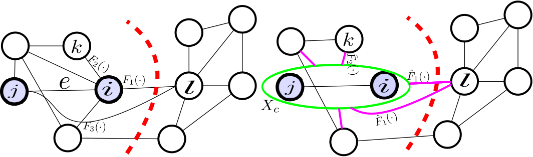
Instead of computing the one-to-one connectivity measure between a node and all other nodes, the abstraction strategy computes the expected value of of the node and a group of nodes that are similar to each other:
| (14) | ||||
| (15) |
where is the set of nodes in the graph, is a particular node in the group of similar nodes , and encodes the expectation function. The value of is approximately equal to the actual value of since the is the combination of nodes that are similar to each other. Furthermore, even if this approximation does deviate from the actual value of , the nodes that are similar to each other are on the same side of the cut with high probability since they are grouped together as and have zero value of between each other while have larger values (greater than zero or zero for exactly similar ones) of with outside nodes of . As such computing the expected value instead of the actual value does not change the relationship amongst the nodes inside the set and the outside nodes; therefore, the individual final cut edges are not changed based on the aforementioned theorem. It is worth noting that the intra-edges in the group of similar nodes have very large connectivity measures such that their corresponding edges have very low probability to be a cut edge. Therefore, the proposed abstraction strategy has a very low probability of changing the actual cut edges of the problem.
As shown in the right graph of Figure 3, instead of computing the connectivity measure between node and nodes and respectively, the abstraction strategy approximates these functions as , the expected value based on a set of the nodes which consists nodes and . Using this strategy, only one computation is done to approximate the connectivity measure between node and all nodes in the set .
III Results & Discussion
The performance of the proposed probabilistic graphical modeling framework was compared with that of different state-of-the-art random field inference frameworks for the problem of interactive image segmentation. The three different realizations of the proposed framework as discussed in Section II-D were evaluated to investigate the tradeoff between the use of different f-divergence measures. Natural images from the complex scene saliency dataset (CSSD) [36], the Microsoft research interactive dataset (MRIS) [37], and the fine structures dataset (MSRA-FS) [20] were used in this evaluation. The CSSD, MRIS and MSRA-FS datasets contain 200, 50 and 30 images respectively. The segmentation procedure is conducted based on user-specified areas as seed points corresponding to the object of interest and the background.
The MSRA-FS images were chosen as the validation set to find the optimal parameters through a grid search procedure. The same parameters are used for different realizations of the proposed framework for the purpose of comparison to maintain consistency. To investigate the performance of the proposed framework compared to existing state-of-the-art random field inference frameworks, we also tested the principled deep random field (PD) framework [15], which utilizes higher-order pairwise penalty functions, and the dense CRF (DCRF) [25], which utilizes fully-connected CRFs via Permutohedral lattices. The implementations of these two frameworks are provided by the corresponding authors via the source code their authors had provided publicly. The reported optimal parameters of the PD framework were consistent with the optimal solution of the tested datasets. However, the reported optimal parameters of DCRF had not produced the best result for the tested datasets and so the parameters were selected based on a grid search procedure to find the optimal solution.
For the proposed framework, we utilize the following pairwise potential function :
| (16) |
where is defined as follows for 4-connected cliques:
| (17) |
where is a controlling parameter, and is defined as follows for long-range cliques:
| (18) |
where the is the controlling parameter. The use of such a potential function illustrates the ability of the proposed framework to utilize arbitrary potential functions without limitations to specific potential functions (e.g., Gaussian potentials).
The neighborhood statistics of each node in the image was computed based on a neighborhood size of centered by the interested node in all realizations of the proposed framework.
The reported results in section III-A were conducted based on the configuration of the proposed framework where the expected number of connectivities per node is 30 cliques. It is worth noting that this number of cliques per node satisfies the conditions discussed in section II-C1
As described in Section II-E it is necessary to determine the set of () for approximating connectivity measures using the abstraction strategy. Here, for the problem of image segmentation and for the sake of computational efficiency, a set of sets (denoted by ) is determined by finding the optimal sets of nodes such that the -norm between the encoded statistics and relative positions of the nodes within the sets and their corresponding set means is minimized
| (19) |
where and are the encoded statistics and relative position corresponding to node , respectively, and and denote the means of the encoded statistics and relative positions of the nodes within the set , respectively. Based on empirical testing, sets was found to provide strong segmentation performance.
All methods are examined and compared quantitatively using three different performance metrics: i) Region F1-Score, ii) Boundary F1-score, and iii) Intersection over union (IOU) [38]. The F1-score is formulated as
| (20) |
where , and are the number of true positives, false negatives, and false positives, respectively. Note that the boundary F1-score [39] is evaluated based on a 2-pixel tolerance. IOU is the intersection of the estimated segmentation result per class and the ground truth, divided by the union:
| (21) |
All realizations of the proposed framework were implemented in a graph cuts framework. The connectivity measure is computed by use of the proposed abstraction approach (section II-E) for all realizations of the proposed framework with the exception of the Bregman Divergence realization, which is realized based on that presented in our preliminary work [19] as a baseline reference. From this point on, BD, HD, and KLD will denote the Bregman Divergence, Hellinger Distance, and KL-Divergence realizations of the proposed framework.
III-A Experimental Results
Tables I and II show quantitative comparisons of the tested methods in terms of the region F1-score and the boundary F1-score. As seen, the different realizations of the proposed framework achieve competitive performance when compared to the tested state-of-the-art PD and DCRF frameworks, and even outperforms them in certain datasets. As illustrated in Table II, the different realizations of the proposed framework was able to preserve boundaries as well as the regions of interest with good accuracy when compared to the other frameworks. From Table III, it can be seen that the reported results of the intersection over union (IOU) show a similar trend as the region F1-score results of Table I. The average score rows in Tables I, II and III illustrate that the proposed framework provides strong overall performance when compared to other compared state-of-the-art approaches based on the different quantitative performance metrics.
Table I reports the computational run-time of the compared frameworks. By comparing the computational complexity of the BD realization and two other realizations, it can be concluded that utilizing the abstraction strategy helps to capture more informative cliques while also decreasing the computational complexity of the graph cuts procedure. It can be observed that all realizations of the proposed framework achieved lower running times when compared to the PD framework which is implemented using a combination of MATLAB with MEX as with the proposed framework. It can be concluded that the proposed framework is efficient and reasonably fast enough according to its implementation.
| DCRF [9] | PD [15] | BD [19] | HD | KLD | |
|---|---|---|---|---|---|
| CSSD | 0.8551 | 0.8286 | 0.8268 | 0.8625 | 0.8624 |
| MRIS | 0.8717 | 0.9032 | 0.8756 | 0.8862 | 0.8861 |
| MSRA-FS | 0.8764 | 0.8592 | 0.8618 | 0.8702 | 0.8707 |
| Average | 0.8677 | 0.8636 | 0.8547 | 0.8729 | 0.8730 |
| Implement. | C++ | M+M | M+M | M+M | M+M |
| Time (s) | 0.48 | 17.512 | 5.275 | 2.431 | 2.494 |
| DCRF [9] | PD [15] | BD [19] | HD | KLD | |
|---|---|---|---|---|---|
| CSSD | 0.5212 | 0.5349 | 0.5235 | 0.5659 | 0.5655 |
| MRIS | 0.5452 | 0.6389 | 0.6175 | 0.6133 | 0.6121 |
| MSRA-FS | 0.5991 | 0.5413 | 0.5371 | 0.5731 | 0.5746 |
| Average | 0.5551 | 0.5715 | 0.5593 | 0.5841 | 0.5840 |
Example segmentation results produced by the tested frameworks for the different datasets are shown in Figure 4. It can be seen that the PD framework has difficulties in preserving boundaries in the test cases shown, with either the background being merged with the object or parts of the object being classified as background (particularly in the “Tree” image (sixth row) and the “Reclining Girl” image (second row). DCRF was able to preserve boundaries better than PD for both the “Standing girl” (fifth row) and “Reclining girl” images; however, the results produced by DCRF exhibited additional segmentation artifacts seen in “Monk” image (third row) and the ”Man with hat” image (fourth row). It can be observed that the proposed framework is capable of preserving narrow and elongated boundaries, as evident by the preservation of the tree stem in the ”Tree” image by the KLD and HD realizations and the dog’s eye and nose in the ”Dog” image (first row) by all realizations of the proposed framework. Furthermore, it can be observed that the proposed framework is capable of dealing with scenarios characterized by complex and cluttered backgrounds, as evident by ”Tree” and “Man with hat” images.
| DCRF [9] | PD [15] | BD [19] | HD | KLD | |
|---|---|---|---|---|---|
| CSSD | 0.7626 | 0.7306 | 0.7328 | 0.7740 | 0.7739 |
| MRIS | 0.7912 | 0.8320 | 0.8057 | 0.8091 | 0.8092 |
| MSRA-FS | 0.7953 | 0.7287 | 0.7737 | 0.7846 | 0.7852 |
| Average | 0.7830 | 0.7637 | 0.7707 | 0.7892 | 0.7894 |
 |
 |
 |
 |
 |
 |
 |
 |
 |
 |
 |
 |
 |
 |
 |
 |
 |
 |
 |
 |
 |
 |
 |
 |
 |
 |
 |
 |
 |
 |
 |
 |
 |
 |
 |
 |
 |
 |
 |
 |
 |
 |
| (a) Image | (b) Ground Truth | (c) DCRF | (d) PD | (e) BD | (g) KLD | (h) HD |
IV Conclusion
In this work, a generalized probabilistic modeling framework based on the concept of stochastic cliques was proposed to facilitate for the use of fully-connected CRFs for structured inference in a computationally tractable manner without additional restrictions or limitations on potential functions being imposed. It is illustrated that the proposed framework provides competitive performance for the purpose of image segmentation when compared to existing fully-connected random field frameworks and the principled deep random field framework, which are considered to be state-of-the-art in the random field frameworks for image segmentation. Although the reported results are based on the use of the standard graph cuts inference approach, the proposed framework can be utilized within different inference approaches, which is a worthy direction for future investigations.
Acknowledgment
This work was supported by the Natural Sciences and Engineering Research Council of Canada, Canada Research Chairs Program, and the Ontario Ministry of Research and Innovation.
References
- [1] B. Fulkerson, A. Vedaldi, and S. Soatto, “Class segmentation and object localization with superpixel neighborhoods,” in International Conference on Computer Vision (ICCV). IEEE, 2009.
- [2] J. Shotton, J. Winn, C. Rother, and A. Criminisi, “Textonboost for image understanding: Multi-class object recognition and segmentation by jointly modeling texture, layout, and context,” International Journal of Computer Vision (IJCV). Springer, 2009.
- [3] A. Blake, P. Kohli, and C. Rother, Markov random fields for vision and image processing. Mit Press, 2011.
- [4] V. Lempitsky and Y. Boykov, “Global optimization for shape fitting,” in Computer Vision and Pattern Recognition, 2007. CVPR’07. IEEE Conference on. IEEE, 2007, pp. 1–8.
- [5] L. Ladicky, C. Russell, P. Kohli, and P. Torr, “Associative hierarchical crfs for object class image segmentation,” in International Conference on Computer Vision (ICCV). IEEE, 2009.
- [6] P. Kohli, P. Torr et al., “Robust higher order potentials for enforcing label consistency,” International Journal of Computer Vision. Springer, 2009.
- [7] X. He, R. Zemel, and M. Carreira-Perpindn, “Multiscale conditional random fields for image labeling,” in Conference on Computer vision and pattern recognition (CVPR). IEEE, 2004.
- [8] A. Rabinovich, A. Vedaldi, C. Galleguillos, E. Wiewiora, and S. Belongie, “Objects in context,” in International Conference on Computer Vision. IEEE, 2007.
- [9] P. Krähenbühl and V. Koltun, “Efficient inference in fully connected CRFs with gaussian edge potentials,” in Advances in Neural Information Processing Systems (NIPS), 2011.
- [10] A. Adams, J. Baek, and M. Davis, “Fast high-dimensional filtering using the permutohedral lattice,” in Computer Graphics Forum. Wiley Online Library, 2010.
- [11] K. Ristovski, V. Radosavljevic, S. Vucetic, and Z. Obradovic, “Continuous conditional random fields for efficient regression in large fully connected graphs,” in Conference on Artificial Intelligence (AAAI), 2013.
- [12] Y. Zhang and T. Chen, “Efficient inference for fully-connected CRFs with stationarity,” in Conference on Computer Vision and Pattern Recognition (CVPR). IEEE, 2012.
- [13] S. Zheng, M. Cheng, J. Warrell, P. Sturgess, V. Vineet, C. Rother, and P. Torr, “Dense semantic image segmentation with objects and attributes,” in International Conference on Computer Vision (ICCV). IEEE, 2014.
- [14] S. Jegelka and J. Bilmes, “Submodularity beyond submodular energies: coupling edges in graph cuts,” in Conference on Computer Vision and Pattern Recognition (CVPR). IEEE, 2011.
- [15] P. Kohli, A. Osokin, and S. Jegelka, “A principled deep random field model for image segmentation,” in Conference on Computer Vision and Pattern Recognition (CVPR). IEEE, 2013.
- [16] B. Bollobás and F. Chung, Probabilistic combinatorics and its applications. American Mathematical Soc., 1991.
- [17] D. Karger, “Random sampling in graph optimization problems,” stanford university, 1995.
- [18] A. Benczúr and D. Karger, “Randomized approximation schemes for cuts and flows in capacitated graphs,” SIAM Journal on Computing, vol. 44, no. 2, pp. 290–319, 2015.
- [19] M. J. Shafiee, A. Wong, P. Siva, and P. Fieguth, “Efficient bayesian inference using fully connected conditional random fields with stochastic cliques,” in IEEE International Conference on Image Processing (ICIP)., 2014, pp. 1–5.
- [20] M. J. Shafiee, A. G. Chung, A. Wong, and P. Fieguth, “Improved fine structure modeling via guided stochastic clique formation in fully connected conditional random fields,” in IEEE International Conference on Image Processing (ICIP)., 2015, pp. 1–5.
- [21] P. Clifford, “Markov random fields in statistics,” Disorder in physical systems: A volume in honour of John M. Hammersley, pp. 19–32, 1990.
- [22] S. Geman and D. Geman, “Stochastic relaxation, gibbs distributions, and the bayesian restoration of images,” Pattern Analysis and Machine Intelligence, IEEE Transactions on, no. 6, pp. 721–741, 1984.
- [23] R. Klinger and K. Tomanek, Classical probabilistic models and conditional random fields. TU, Algorithm Engineering, 2007.
- [24] A. Blake, P. Kohli, and C. Rother, Markov random fields for vision and image processing. Mit Press, 2011.
- [25] P. Krähenbühl and V. Koltun, “Efficient inference in fully connected crfs with gaussian edge potentials,” in Advances in Neural Information Processing Systems, 2011.
- [26] Y. Zhang and T. Chen, “Efficient inference for fully-connected crfs with stationarity,” in Computer Vision and Pattern Recognition (CVPR), 2012 IEEE Conference on. IEEE, 2012, pp. 582–589.
- [27] K. Ristovski, V. Radosavljevic, S. Vucetic, and Z. Obradovic, “Continuous conditional random fields for efficient regression in large fully connected graphs,” in Twenty-Seventh AAAI Conference on Artificial Intelligence, 2013.
- [28] P. Erdos and A. Renyi, “On random graphs i.” Publ. Math. Debrecen, 1959.
- [29] F. Chung and L. Lu, Complex graphs and networks. American mathematical society Providence, 2006.
- [30] I. N. Kovalenko, “The structure of random directed graph,” Probab. Math. Statist., 1975.
- [31] K. Iverson, “A programming language,” in Proceedings of the May 1-3, 1962, spring joint computer conference. ACM, 1962, pp. 345–351.
- [32] Y. Boykov and M.-P. Jolly, “Interactive graph cuts for optimal boundary & region segmentation of objects in nd images,” in International Conference on Computer Vision (ICCV). IEEE, 2001.
- [33] F. Liese and I. Vajda, “On divergences and informations in statistics and information theory,” Information Theory, IEEE Transactions on, vol. 52, no. 10, pp. 4394–4412, 2006.
- [34] H. Nagamochi and T. Ibaraki, “A linear-time algorithm for finding a sparsek-connected spanning subgraph of ak-connected graph,” Algorithmica, vol. 7, no. 1-6, pp. 583–596, 1992.
- [35] ——, “Computing edge-connectivity in multigraphs and capacitated graphs,” SIAM Journal on Discrete Mathematics, vol. 5, no. 1, pp. 54–66, 1992.
- [36] Q. Yan, L. Xu, J. Shi, and J. Jia, “Hierarchical saliency detection,” in Computer Vision and Pattern Recognition (CVPR). IEEE, 2013.
- [37] C. Rother, V. Kolmogorov, and A. Blake, “Grabcut: Interactive foreground extraction using iterated graph cuts,” ACM Transactions on Graphics (TOG), vol. 23, no. 3, pp. 309–314, 2004.
- [38] M. Everingham, A. Eslami, L. Van Gool, C. Williams, J. Winn, and A. Zisserman, “The pascal visual object classes challenge: A retrospective,” International Journal of Computer Vision, vol. 111, no. 1, pp. 98–136, 2014.
- [39] P. Arbelaez, M. Maire, C. Fowlkes, and J. Malik, “Contour detection and hierarchical image segmentation,” IEEE Transactions on Pattern Analysis and Machine Intelligence, vol. 33, no. 5, pp. 898–916, 2011.