跳到论文正文
W Papers独立论文阅读器 arXiv:1506.08793 论文正文 计算阅读时间 · 0%
引用这篇论文根据当前论文元数据生成,正式投稿前建议核对。


License: arXiv.org perpetual non-exclusive license
arXiv:1506.08793v1 [math.AG] 29 Jun 2015

Projectivity of Bridgeland Moduli Spaces on Del Pezzo Surfaces of Picard Rank 2

Daniele Arcara    Eric Miles
Abstract

We prove that, for a natural class of Bridgeland stability conditions on ℙ1×ℙ1{\mathbb{P}}^{1}\times{\mathbb{P}}^{1} and the blow-up of ℙ2{\mathbb{P}}^{2} at a point, the moduli spaces of Bridgeland semistable objects are projective. Our technique is to find suitable regions of stability conditions with hearts that are (after “rotation”) equivalent to representations of a quiver. The helix and tilting theory is well-behaved on Del Pezzo surfaces and we conjecture that this program (begun in [ABCH13]) runs successfully for all Del Pezzo surfaces, and the analogous Bridgeland moduli spaces are projective.

1 Introduction

Let SS be a smooth projective complex surface and D​(S)=Db​(Coh ​S)D(S)=D^{b}({\textrm{Coh\,}}S) be its associated bounded derived category. A Bridgeland stability condition σ\sigma gives a notion of stability for objects of D⁡(S)D(S) and it is interesting to study the moduli space ℳσ​(v){\mathcal{M}}_{\sigma}(v) of σ\sigma-semistable objects of Chern character vv.

Unlike Mumford and Gieseker stability, Bridgeland stability conditions are not a priori tied to Geometric Invariant Theory (GIT), and consequently the structure of Bridgeland moduli spaces ℳσ​(v){\mathcal{M}}_{\sigma}(v) is not fully understood in general, e.g., are they projective? A general approach to this question is taken in [BM14] where Bayer and Macrì construct nef divisors on Bridgeland moduli spaces and show that for K3 surfaces, the divisors are ample.

Another method to deduce structure for these moduli spaces is to find particular stability conditions that have ties to GIT, and exploit this connection. For example, the first author and Bertram [AB13] define a class of stability condition defined by a choice of general and ample divisor in SS. When SS has Picard rank 1, the space of these stability conditions is parameterized by real variables, s,ts,t with t>0t>0, and for large tt Bridgeland stability is equivalent to Gieseker stability (e.g. [ABCH13, Proposition 6.2]) and thus the corresponding Bridgeland moduli spaces have a GIT interpretation and are projective.

For SS a principally polarized abelian surface, Maciocia and Meachan [MM13] use this connection to deduce projectivity for other Bridgeland stability conditions by “sliding down the wall”: for invariants corresponding to twisted ideal sheaves, they show that one can move a stability condition (taken from a 1-parameter family of stability conditions) so that tt is arbitrarily small without crossing any walls for those invariants (the walls are nested semi-circles centered on the ss-axis). They conclude projectivity by relating stability conditions with small tt to those with large tt via a Fourier-Mukai transform.

For S=ℙ2S={\mathbb{P}}^{2}, the first author, Bertram, Coskun, and Huizenga [ABCH13] find stability conditions with small tt where Bridgeland stability for complexes of sheaves is equivalent to King’s χ\chi-stability for representations of a quiver [Kin94]. By a result of King, it follows that the associated Bridgeland moduli spaces are projective. To extend this structure to other stability conditions, they show that for invariants satisfying the Bogomolov inequality, one can “slide down the wall” and see the original Bridgeland moduli space as isomorphic to one associated to a stability condition with small tt.

The quivers involved in [ABCH13] are associated to certain exceptional collections of objects in Db​(ℙ2)D^{b}({\mathbb{P}}^{2}). These exceptional collections exist on other surfaces, e.g., Del Pezzo surfaces, but the “quiver regions” associated to the most natural exceptional collections are too small. Furthermore, determining new exceptional collections is difficult, as the action of the Artin braid group on the set of exceptional collections for ℙ2{\mathbb{P}}^{2} does not apply when dimK⁡(S)⊗ℂ>1+dimS\dim K(S)\otimes{\mathbb{C}}>1+\dim S, which is the case for all other Del Pezzos.

However, Bridgeland and Stern [BS10] describe an operation (called mutation defined by a height function) which produces new exceptional collections in this more general setting (and matches the action of the braid group when S=ℙ2S={\mathbb{P}}^{2}). This operation is applicable for any smooth Fano variety, but works in an ideal way on Del Pezzo surfaces. We look to extend the techniques of [ABCH13] to the other Del Pezzo surfaces.

Conjecture 1.

The program of [ABCH13] can be carried out on any Del Pezzo surface SS, yielding the projectivity of the spaces ℳσ​(v){\mathcal{M}}_{\sigma}(v).

For the Del Pezzo surfaces of Picard rank 2, S=ℙ1×ℙ1S={\mathbb{P}}^{1}\times{\mathbb{P}}^{1} and S=B​lp​ℙ2S=Bl_{p}{\mathbb{P}}^{2}, we find stability conditions that, after an operation called “rotation,” have their hearts equivalent to a category of quiver representations. These hearts are generated by (shifts of) line bundles for S=ℙ1×ℙ1S={\mathbb{P}}^{1}\times{\mathbb{P}}^{1} and (shifts of) line bundles and a torsion sheaf for S=B​lp​ℙ2S=Bl_{p}{\mathbb{P}}^{2}. Understanding the Bridgeland stability of these objects is essential to finding these “quiver stability conditions,” and while the stability of line bundles is fully understood for these surfaces [AM14], a full characterization of their stability is not known when the surface has Picard rank greater than 2.

Following [ABCH13], Bridgeland stability for these quiver stability conditions is equivalent to King’s stability of representations of a quiver and we deduce projectivity for the associated moduli spaces of Bridgeland semi-stable objects. To extend this structure to moduli spaces associated to other stability conditions we “slide down the wall,” using a result of Maciocia on the nestedness of walls in certain vertical planes in the space of stability conditions.

Our main theorem is the following.

Theorem 1.1.

The conjecture is true for S=ℙ1×ℙ1S={\mathbb{P}}^{1}\times{\mathbb{P}}^{1} and S=B​lp​ℙ2S=Bl_{p}{\mathbb{P}}^{2}, which are Del Pezzo surfaces of Picard Rank 22. In particular, every moduli space ℳσ​(v){\mathcal{M}}_{\sigma}(v) is equivalent to a moduli space of representations of a quiver, and is therefore projective.

The paper is organized as follows. In Section 2, we recall some of the definitions and tools that are needed in the rest of the paper. In Section 3 we describe our strategy. In Section 4 we prove the conjecture for S=ℙ1×ℙ1S={\mathbb{P}}^{1}\times{\mathbb{P}}^{1}. Finally, in Section 5, we prove the conjecture for S=B​lp​ℙ2S=Bl_{p}{\mathbb{P}}^{2}.

2 Useful definitions

In this section, we recall definitions and tools that we need in the rest of the paper.

2.1 Bridgeland stability conditions on surfaces

For SS a smooth projective complex surface, [AB13] define a natural class of Bridgeland stability conditions that depend on a choice of ample and general divisor. We denote the set of such Bridgeland stability conditions Stabd​i​v​(S)\text{Stab}_{div}(S) (the “div” stands for “divisor”). We omit a general introduction to Bridgeland stability conditions and instead point out where the [AB13] construction meets the requirements “as we go.” For full generality, the interested reader should see [Bri07].

Let SS be a smooth projective surface. Given two ℝ{\mathbb{R}}-divisors D,HD,H with HH ample, we define a stability condition σD,H\sigma_{D,H}. To do so, we must specify a heart 𝒜D,H{\mathcal{A}}_{D,H} of a bounded tt-structure on D⁡(S)D(S) and a function ZD,H:Kn​u​m​(S)→ℂZ_{D,H}:K_{num}(S)\to{\mathbb{C}} (called the central charge) satisfying certain positivity, filtration, and non-degenerate conditions.

Our heart is generated by torsion sheaves, Mumford HH-stable sheaves of “high slope,” and shifts of Mumford HH-stable sheaves of “low slope,” where the Mumford HH-slope is

μH​(G)=c1​(G).Hrk​(G)​H2.\mu_{H}(G)=\displaystyle\frac{c_{1}(G).H}{{\textrm{rk}}(G)H^{2}}.

Specifically, let 𝒜D,H{\mathcal{A}}_{D,H} be the tilt of the standard tt-structure on D⁡(S)D(S) at μH​(D)=D.HH2\mu_{H}(D)=\displaystyle\frac{D.H}{H^{2}} defined by 𝒜D,H={G∈D(S)∣Hi(G)=0 for i≠−1,0,H−1(G)∈ℱD,H,H0(G)∈𝒯D,H}{\mathcal{A}}_{D,H}=\{G\in D(S)\mid H^{i}(G)=0\text{ for }i\neq-1,0,\ H^{-1}(G)\in{\mathcal{F}}_{D,H},\ H^{0}(G)\in{\mathcal{T}}_{D,H}\} where

  • •

    𝒯D,H⊂Coh ​(S){\mathcal{T}}_{D,H}\subset{\textrm{Coh\,}}(S) is the full subcategory closed under extensions generated by torsion sheaves and μH\mu_{H}-stable sheaves GG with μH​(G)>D.HH2\mu_{H}(G)>\displaystyle\frac{D.H}{H^{2}}.

  • •

    ℱD,H⊂Coh ​(S){\mathcal{F}}_{D,H}\subset{\textrm{Coh\,}}(S) is the full subcategory closed under extensions generated by μH\mu_{H}-stable sheaves GG with μH​(G)≤D.HH2\mu_{H}(G)\leq\displaystyle\frac{D.H}{H^{2}}.

Now define ZD,HZ_{D,H} by ZD,H(G)=−∫e−(D+i​H)ch(G).Z_{D,H}(G)=-\displaystyle\int{e^{-(D+iH)}{\textrm{ch}}(G)}. It is equal to

ZD,H(G)=(−ch2(G)+c1(G).D−rk​(G)2(D2−H2))+i(c1(G).H−rk(G)D.H)Z_{D,H}(G)=\left(-{\textrm{ch}}_{2}(G)+c_{1}(G).D-\frac{{\textrm{rk}}(G)}{2}(D^{2}-H^{2})\right)+i\left(c_{1}(G).H-{\textrm{rk}}(G)D.H\right)

The central charge ZD,HZ_{D,H} satisfies the following positivity property: for 0≠G∈𝒜D,H0\neq G\in{\mathcal{A}}_{D,H} we have Im ​Z​(G)≥0{\textrm{Im\,}}Z(G)\geq 0 and if Im ​Z​(G)=0{\textrm{Im\,}}Z(G)=0 then Re ​Z​(G)<0{\textrm{Re\,}}Z(G)<0. This property allows us to define stability for an object G∈𝒜D,HG\in{\mathcal{A}}_{D,H} using the “Bridgeland slope” function

β(G)=−Re ​Z​(G)Im ​Z​(G)∈(−∞,∞]\beta(G)=-\frac{{\textrm{Re\,}}Z(G)}{{\textrm{Im\,}}Z(G)}\in(-\infty,\infty]

(Note that if Z⁡(G)=−1Z(G)=-1 then β⁡(G)=∞\beta(G)=\infty, and if Z⁡(G)=−1Z(G)=\sqrt{-1} then β⁡(G)=0\beta(G)=0.) We say that G∈𝒜D,HG\in{\mathcal{A}}_{D,H} is σD,H\sigma_{D,H}-stable (resp. σD,H\sigma_{D,H}-semistable) if for all nontrivial G′⊂GG^{\prime}\subset G in 𝒜D,H{\mathcal{A}}_{D,H} we have β⁡(G)>β⁡(G′)\beta(G)>\beta(G^{\prime}) (resp. β⁡(G)≥β⁡(G′)\beta(G)\geq\beta(G^{\prime})). We extend the notion of stability to all objects of the derived category: G∈D⁡(S)G\in D(S) is σD,H\sigma_{D,H}-(semi)stable if some shift G⁡[k]∈𝒜D,HG[k]\in{\mathcal{A}}_{D,H} and G⁡[k]G[k] is σD,H\sigma_{D,H}-(semi)stable.

There exist Harder-Narasimhan filtrations of objects G∈𝒜D,HG\in{\mathcal{A}}_{D,H} with respect to σD,H\sigma_{D,H}-semistable objects, defined analogously to Harder-Narasimhan filtrations of coherent sheaves with respect to Mumford HH-semistable sheaves. By [AB13, Corollary 2.1] and [Tod13, Sections 3.6 & 3.7], σD,H\sigma_{D,H} is a full, numerical stability condition on SS.

2.2 Exceptional collections and associated hearts

Here we describe the heart and quiver associated to a full, strong exceptional collection, as well as an operation that (in certain circumstances) yields new collections from others. We use E⋆E_{\star} instead of EE to denote a particular exceptional object since in Section 5 we use EE for the exceptional divisor of B​lp​ℙ2Bl_{p}{\mathbb{P}}^{2}.

An exceptional object E⋆∈D⁡(S)E_{\star}\in D(S) is one with Hom0​(E⋆,E⋆)=ℂ\text{Hom}^{0}(E_{\star},E_{\star})={\mathbb{C}} and Homi​(E⋆,E⋆)=0\text{Hom}^{i}(E_{\star},E_{\star})=0 for all i≠0i\neq 0. For a Del Pezzo surface SS, Kuleshov and Orlov show that any exceptional object EE is either a Mumford −KS-K_{S}-stable locally-free sheaf or a torsion sheaf of the form 𝒪C​(d){\mathcal{O}}_{C}(d) with C⊂SC\subset S an irreducible rational curve satisfying C2=−1C^{2}=-1 and d∈ℤd\in{\mathbb{Z}} an integer (see, e.g. [GK04] or [BS10, Theorem 8.1]). Note that the Del Pezzo condition is not necessary for much of the following discussion (we will make a note where it is used).

An exceptional collection 𝔼⊂D⁡(S){\mathbb{E}}\subset D(S) is a sequence (E1,…,En)(E_{1},\ldots,E_{n}) such that each EiE_{i} is an exceptional object and i<ji<j implies Hom∙​(Ej,Ei)=0\text{Hom}^{\bullet}(E_{j},E_{i})=0. An exceptional collection 𝔼{\mathbb{E}} is called full if the smallest full triangulated subcategory of D⁡(S)D(S) containing 𝔼{\mathbb{E}} is D⁡(S)D(S) itself, and 𝔼{\mathbb{E}} is called strong if for i<ji<j we have Homk​(Ei,Ej)=0\text{Hom}^{k}(E_{i},E_{j})=0 unless k=0k=0.

Bridgeland and Stern show that a full strong exceptional collection yields a heart 𝒜𝔼∈D⁡(S){\mathcal{A}}_{\mathbb{E}}\in D(S) (of a bounded tt-structure) that is equivalent to the module category of a quiver algebra, which in turn is equivalent to the category of finite-dimensional representations of a quiver (possibly with relations) [BS10, Theorem 2.4]. Furthermore, the heart 𝒜𝔼{\mathcal{A}}_{\mathbb{E}} is the smallest full extension-closed subcategory of D⁡(S)D(S) containing the dual collection 𝔽=(Fn,…,F1){\mathbb{F}}=(F_{n},\ldots,F_{1}) to 𝔼{\mathbb{E}} (for this reason we often denote 𝒜𝔼{\mathcal{A}}_{\mathbb{E}} by 𝒜𝔽{\mathcal{A}}_{\mathbb{F}}). The objects FiF_{i} are defined by Fi=LE1LE2⋯LEi−1(Ei)F_{i}=L_{E_{1}}L_{E_{2}}\cdots L_{E_{i-1}}(E_{i}), where LA​BL_{A}B is the left mutation of BB through AA defined by the canonical evaluation triangle:

Hom∙​(A,B)⊗A→B→LA​B.\text{Hom}^{\bullet}(A,B)\otimes A\to B\to L_{A}B.

The quiver associated to the heart 𝒜𝔼{\mathcal{A}}_{\mathbb{E}} has a vertex associated to each EiE_{i}. The number of arrows ni​jn_{ij} from vertex ii to vertex jj can be obtained using either irreducible hom’s between objects in 𝔼{\mathbb{E}} or extensions of objects in 𝔽{\mathbb{F}}:

  • •

    ni​j=dim coker ​⨁i<k<jHom​(Ei,Ek)⊗Hom​(Ek,Ej)→Hom​(Ei,Ej)n_{ij}=\dim\text{ coker }\displaystyle\bigoplus_{i<k<j}\text{Hom}(E_{i},E_{k})\otimes\text{Hom}(E_{k},E_{j})\to\text{Hom}(E_{i},E_{j})

  • •

    ni​j=dimHom1​(Fj,Fi)n_{ij}=\dim\text{Hom}^{1}(F_{j},F_{i})

The objects FiF_{i} correspond to the simple representation over the ithi^{\text{th}} vertex.

Given a full exceptional collection 𝔼=(E1,…,En){\mathbb{E}}=(E_{1},\ldots,E_{n}) one may generate the helix ℍ=(Ei)i∈ℤ{\mathbb{H}}=(E_{i})_{i\in{\mathbb{Z}}} using the rule Ei−n=Ei⊗ωSE_{i-n}=E_{i}\otimes\omega_{S}. (This generates a helix of type (n,3)(n,3) in the notation of [BS10].) The helix ℍ{\mathbb{H}} is said to be geometric if i<ji<j implies Homk​(Ei,Ej)=0\text{Hom}^{k}(E_{i},E_{j})=0 unless k=0k=0. If ℍ{\mathbb{H}} is a geometric helix then each “thread” (Ek,…,Ek+n)(E_{k},\ldots,E_{k+n}) is a full strong exceptional collection.

Bridgeland and Stern define an operation on exceptional collections (resp. helices) called mutation defined by a height function for E⋆E_{\star}, which constructs a new exceptional collection 𝔼′{\mathbb{E}}^{\prime} (resp. helix ℍ′{\mathbb{H}}^{\prime}) from a given one 𝔼{\mathbb{E}} (resp. ℍ{\mathbb{H}}) and choice of object E⋆∈𝔼E_{\star}\in{\mathbb{E}} (resp. OPENℍ){\mathbb{H}}). If ℍ{\mathbb{H}} is geometric then so is ℍ′{\mathbb{H}}^{\prime} and it is shown that, if SS is a Del Pezzo surface, then for any choice of object E⋆∈ℍE_{\star}\in{\mathbb{H}} there is an associated height function. We do not formally define this operation here, but direct the interested reader to Appendix A for the precise definition as well as an interpretation using the quiver associated to a thread containing E⋆E_{\star}.

Because the quiver algebra associated to 𝔼′{\mathbb{E}}^{\prime} is the left tilt of that associated to 𝔼{\mathbb{E}} ([BS10, Proposition 7.3]) and since for Del Pezzos the mutation by a height function operation is determined solely by the choice of object EE (see Proposition A.1), we refer to a mutation defined by a height function for EE as a left tilt at EE.

3 Discussion of the strategy

Let us now discuss the specifics of our strategy.

From Section 2.2, a full, strong exceptional collection 𝔼=(E1,…,En){\mathbb{E}}=(E_{1},\ldots,E_{n}) with dual collection 𝔽=(Fn,…,F1){\mathbb{F}}=(F_{n},\ldots,F_{1}) yields a heart 𝒜𝔽⊂D⁡(S){\mathcal{A}}_{\mathbb{F}}\subset D(S) that is generated by extensions of the objects FiF_{i}, and equivalent to finite-dimensional representations of a quiver. The exceptional collection 𝔽{\mathbb{F}} is “Ext” in the sense of [Mac07, Definition 3.10] and so by [Mac07, Lemma 3.16], if σ=(Z,𝒜)∈Stabd​i​v​(S)\sigma=(Z,{\mathcal{A}})\in\text{Stab}_{div}(S) and 𝔽⊂𝒜{\mathbb{F}}\subset{\mathcal{A}} then 𝒜=𝒜𝔽{\mathcal{A}}={\mathcal{A}}_{\mathbb{F}}.

A choice of invariants vv corresponds to a choice of dimension vector and following the proof of [ABCH13, Proposition 8.1] we see that σ\sigma-stability is equivalent to King’s χ\chi-stability [Kin94]. Thus the moduli space ℳσ​(v){\mathcal{M}}_{\sigma}(v) of Bridgeland semistable objects is projective when semistable objects are considered (and if only stable objects are considered, the space is quasi-projective).

We want to use the above observations to deduce that ℳσ​(v){\mathcal{M}}_{\sigma}(v) is projective for all σ∈Stabd​i​v​(S)\sigma\in\text{Stab}_{div}(S) and (Bogomolov) vv. The first issue with this strategy is that there is no σ∈Stabd​i​v​(S)\sigma\in\text{Stab}_{div}(S) with 𝔽⊂𝒜{\mathbb{F}}\subset{\mathcal{A}}. This is because all dual collections we consider have objects G⁡[2]G[2] where GG is a sheaf, and these objects cannot belong to any 𝒜{\mathcal{A}} by definition. However, there are stability conditions such that, after a gentle operation called “rotation” (which does not affect stability, but does affect what shift of certain objects belong in the heart), the rotated stability condition σ⁡[ϕ]=(Z⁡[ϕ],𝒜⁡[ϕ])\sigma[\phi]=(Z[\phi],{\mathcal{A}}[\phi]) has 𝔽⊂𝒜⁡[ϕ]{\mathbb{F}}\subset{\mathcal{A}}[\phi].

A rotation is defined as follows: Given σ=(Z,𝒜)∈Stabd​i​v​(S)\sigma=(Z,{\mathcal{A}})\in\text{Stab}_{div}(S) and ϕ∈(0,1)\phi\in(0,1), a rotation by ϕ\phi yields the Bridgeland stability condition σ⁡[ϕ]=(Z⁡[ϕ],𝒜⁡[ϕ])\sigma[\phi]=(Z[\phi],{\mathcal{A}}[\phi]) where Z⁡[ϕ]​(G)=e−ϕ​π​i​Z​(G)Z[\phi](G)=e^{-\phi\pi i}Z(G) and 𝒜⁡[ϕ]{\mathcal{A}}[\phi] is the subcategory closed under extensions generated by the objects

  • •

    GG such that G∈𝒜G\in{\mathcal{A}} is σ\sigma-semistable and arg ​Z​(G)/π>ϕ\text{arg }Z(G)/\pi>\phi,

  • •

    G⁡[1]G[1] such that G∈𝒜G\in{\mathcal{A}} is σ\sigma-semistable and arg ​Z​(G)/π≤ϕ\text{arg }Z(G)/\pi\leq\phi.

In particular, if G∈𝒜G\in{\mathcal{A}} is a σ\sigma-semistable object with arg Z⁡(G)/π≤ϕZ(G)/\pi\leq\phi, then GG is “replaced” by G⁡[1]G[1] in 𝒜⁡[ϕ]{\mathcal{A}}[\phi].

We emphasize that rotation does not affect stability: GG is σ\sigma-(semi)stable iff GG is σ⁡[ϕ]\sigma[\phi]-(semi)stable (recall that GG is σ\sigma-(semi)stable iff G⁡[k]G[k] is σ\sigma-(semi)stable for all kk).

In Sections 4 and 5 we find regions R𝔽R_{\mathbb{F}} associated to a dual collection 𝔽{\mathbb{F}} (where after a rotation by ϕ\phi, we have 𝒜⁡[ϕ]=𝒜𝔽{\mathcal{A}}[\phi]={\mathcal{A}}_{\mathbb{F}}). We call R𝔽R_{\mathbb{F}} a quiver region and any σ∈R𝔽\sigma\in R_{\mathbb{F}} a quiver stability condition. We find R𝔽R_{\mathbb{F}} by determining the stability conditions σ\sigma such that each object (or shift of an object) in 𝔽{\mathbb{F}} is σ\sigma-semistable and where the objects have the correct Bridgeland slopes relative to each other so that after rotating we have 𝔽⊂𝒜⁡[ϕ]{\mathbb{F}}\subset{\mathcal{A}}[\phi].

After finding a quiver region R𝔽R_{\mathbb{F}}, any choice of line bundle LL yields the quiver region R𝔽⊗LR_{{\mathbb{F}}\otimes L} associated to the exceptional collection 𝔼⊗L=(E1⊗L,…,En⊗L){\mathbb{E}}\otimes L=(E_{1}\otimes L,\ldots,E_{n}\otimes L). Our discussion above shows that for any quiver stability condition σ\sigma and choice of invariants vv, we have ℳσ​(v){\mathcal{M}}_{\sigma}(v) projective. To extend this projectivity to other stability conditions, we “slide down the wall” in the following sense.

In [Mac14], Maciocia presents real 3-dimensional slices of Stabd​i​v​(S)\text{Stab}_{div}(S) determined by a choice of an ample ℝ{\mathbb{R}}-divisor HH and a divisor orthogonal to HH. When SS has Picard rank 2, these slices are determined solely by HH, and are defined as

𝒮H={σD,t​H|Dℝ-divisor,t>0}.{\mathcal{S}}_{H}=\{\sigma_{D,tH}|D\ {\mathbb{R}}\text{-divisor},t>0\}.

We parametrize 𝒮H{\mathcal{S}}_{H} with the coordinates (x,y,t)(x,y,t) where the x​yxy-plane is a parametrization of DD in N​S​(S)⊗ℝNS(S)\otimes{\mathbb{R}}.

To determine σ\sigma-stability of objects and relative Bridgeland slopes, we must consider walls

𝒲⁡(G,G′)={σ∈Stabd​i​v​(S)|β⁡(G)=β⁡(G′)}.{\mathcal{W}}(G,G^{\prime})=\{\sigma\in\text{Stab}_{div}(S)|\beta(G)=\beta(G^{\prime})\}.

Maciocia shows that there are disjoint vertical11 1 By “vertical” we mean defined by an equation involving only xx and yy. planes Πu⊂𝒮H\Pi_{u}\subset{\mathcal{S}}_{H} depending on a real parameter uu such that ⋃u∈ℝΠu=𝒮H\bigcup_{u\in{\mathbb{R}}}\Pi_{u}={\mathcal{S}}_{H}, and such that for any object GG whose Chern characters satisfy the Bogomolov inequality, the walls 𝒲⁡(G,_)∩Πu{\mathcal{W}}(G,\_)\cap\Pi_{u} are nested semi-circles (or vertical lines) [Mac14, Proposition 2.6].

Refer to caption
Figure 1: Nested walls in Πu⊂𝒮H\Pi_{u}\subset{\mathcal{S}}_{H}

Any σ∈Πu\sigma\in\Pi_{u} lies on at most one of these nested semi-circles, say 𝒲=𝒲⁡(G,G′)∩Πu{\mathcal{W}}={\mathcal{W}}(G,G^{\prime})\cap\Pi_{u}. Since moving along 𝒲{\mathcal{W}} crosses no other walls 𝒲⁡(G,_){\mathcal{W}}(G,\_), for σ,σ′∈𝒲\sigma,\sigma^{\prime}\in{\mathcal{W}} we have GG σ\sigma-(semi)stable iff GG σ′\sigma^{\prime}-(semi)stable. More generally, since the walls 𝒲⁡(G,_)=𝒲⁡(v,_){\mathcal{W}}(G,\_)={\mathcal{W}}(v,\_) are determined by the invariants of the objects involved, for σ,σ′∈𝒲\sigma,\sigma^{\prime}\in{\mathcal{W}} we have ℳσ​(v)=ℳσ′​(v){\mathcal{M}}_{\sigma}(v)={\mathcal{M}}_{\sigma^{\prime}}(v).

Thus, if 𝒲⊂Πu{\mathcal{W}}\subset\Pi_{u} intersects a quiver region, then ℳσ​(v)=ℳσ′​(v){\mathcal{M}}_{\sigma}(v)={\mathcal{M}}_{\sigma^{\prime}}(v) for some quiver stability condition σ′\sigma^{\prime} and hence ℳσ​(v){\mathcal{M}}_{\sigma}(v) is projective. For each of S=ℙ1×ℙ1S={\mathbb{P}}^{1}\times{\mathbb{P}}^{1} and S=B​lp​ℙ2S=Bl_{p}{\mathbb{P}}^{2} we find a quiver region R𝔽R_{\mathbb{F}} such that the quiver regions ℝ𝔽⊗L{\mathbb{R}}_{{\mathbb{F}}\otimes L} cover the entire x​yxy-plane for each 𝒮H{\mathcal{S}}_{H}. Since each σ∈𝒮H\sigma\in{\mathcal{S}}_{H} is in a Πu\Pi_{u} plane, we obtain the projectivity of ℳσ​(v){\mathcal{M}}_{\sigma}(v) for all Bogomolov vv and σ∈Stabd​i​v​(S)\sigma\in\text{Stab}_{div}(S) and thus prove Conjecture 1 in these cases.

We also use the fact that walls 𝒲⁡(v,_){\mathcal{W}}(v,\_) in Πu\Pi_{u} are nested semi-circles for simplification: To understand the geometry of a wall in 𝒮H{\mathcal{S}}_{H} it suffices to consider its intersection with the x​yxy-plane.

4 Proof of the conjecture for S=ℙ1×ℙ1S={\mathbb{P}}^{1}\times{\mathbb{P}}^{1}

In this section, we determine a suitable22 2 Suitable in the sense that the entire x​yxy-plane of 𝒮H{\mathcal{S}}_{H} is covered by tensoring with line bundles. quiver region in Stabd​i​v​(S)\text{Stab}_{div}(S) for S=ℙ1×ℙ1S={\mathbb{P}}^{1}\times{\mathbb{P}}^{1} and use the region to conclude projectivity for the Bridgeland moduli spaces ℳσ​(v){\mathcal{M}}_{\sigma}(v) where the invariants vv satisfy the Bogomolov inequality (following the discussion of Section 3).

We shall denote by 𝒪S​(a,b){\mathcal{O}}_{S}(a,b) the line bundle p1∗​𝒪ℙ1​(a)⊗p2∗​𝒪ℙ1​(b)p_{1}^{*}{\mathcal{O}}_{{\mathbb{P}}^{1}}(a)\otimes p_{2}^{*}{\mathcal{O}}_{{\mathbb{P}}^{1}}(b) with p1,p2p_{1},p_{2} the natural projections from ℙ1×ℙ1{\mathbb{P}}^{1}\times{\mathbb{P}}^{1} to the two copies of ℙ1{\mathbb{P}}^{1}, respectively. Also, we shall denote by D1D_{1} and D2D_{2} the divisors corresponding to 𝒪S​(1,0){\mathcal{O}}_{S}(1,0) and 𝒪S​(0,1){\mathcal{O}}_{S}(0,1), respectively. These are the generators of the cone of effective curves, and every other divisor can be written as x​D1+y​D2xD_{1}+yD_{2} for some x,y∈ℝx,y\in{\mathbb{R}}. Note that D12=D22=0D_{1}^{2}=D_{2}^{2}=0, and D1.D2=1D_{1}.D_{2}=1.

A Bridgeland stability condition σD,H∈Stabd​i​v​(S)\sigma_{D,H}\in\text{Stab}_{div}(S) is determined by real divisor classes D=x​D1+y​D2D=xD_{1}+yD_{2} and H=a​D1+b​D2H=aD_{1}+bD_{2}, with HH ample. By the Nakai-Moishezon criterion, HH is ample iff a,b>0a,b>0.

For a fixed D,HD,H pair, the corresponding Bridgeland stability condition σD,H=σ=(𝒜,Z)\sigma_{D,H}=\sigma=({\mathcal{A}},Z) (we now drop the subscript D,HD,H) has heart 𝒜{\mathcal{A}} generated by μH\mu_{H}-stable sheaves GG of slope μH​(G)>b​x+a​y\mu_{H}(G)>bx+ay, torsion sheaves, and objects of the from G⁡[1]G[1], where GG is a μH\mu_{H}-stable sheaf of slope μH​(G)≤b​x+a​y\mu_{H}(G)\leq bx+ay.

The central charge ZZ is defined as

Z⁡(G)=−ch2​(G)+d2​x+d1​y+r⁡(a​b−x​y)+i⁡(d2​a+d1​b−r⁡(b​x+a​y)),Z(G)=-{\textrm{ch}}_{2}(G)+d_{2}x+d_{1}y+r(ab-xy)+i\left(d_{2}a+d_{1}b-r(bx+ay)\right),

where rk​(G)=r{\textrm{rk}}(G)=r, and c1​(G)=d1​D1+d2​D2c_{1}(G)=d_{1}D_{1}+d_{2}D_{2}.

The slices 𝒮H⊂Stabd​i​v​(S){\mathcal{S}}_{H}\subset\text{Stab}_{div}(S) defined in Section 3 are given here by 𝒮H={σD,t​H|D=x​D1+y​D2​ and ​t>0}{\mathcal{S}}_{H}=\{\sigma_{D,tH}|D=xD_{1}+yD_{2}\text{ and }t>0\}. We identify the Bridgeland stability condition σ=σD,t​H\sigma=\sigma_{D,tH} where D=x​D1+y​D2D=xD_{1}+yD_{2} with the coordinates (x,y,t)(x,y,t). Often we need only consider the xx and yy coordinates, and we project to the the x​yxy-plane.

4.1 A suitable exceptional collection

In the following, we rely on the definitions given in Section 2.2 and the specifics of the “left tilt” operation given in Appendix A.

The natural exceptional collection

𝔼=(𝒪S,𝒪S​(1,0),𝒪S​(0,1),𝒪S​(1,1)){\mathbb{E}}=({\mathcal{O}}_{S},\ {\mathcal{O}}_{S}(1,0),\ {\mathcal{O}}_{S}(0,1),\ {\mathcal{O}}_{S}(1,1))

on ℙ1×ℙ1{\mathbb{P}}^{1}\times{\mathbb{P}}^{1} is full and strong (and in fact generates a geometric helix), but does not have a large enough quiver region for our purposes, so we find another exceptional collection. The quiver associated to 𝔼{\mathbb{E}} is

∙𝒪S{\lx@inpgf@ignorespaces\overset{{\mathcal{O}}_{S}}{\bullet}}∙𝒪S​(1,0){\lx@inpgf@ignorespaces\overset{{\mathcal{O}}_{S}(1,0)}{\bullet}}∙𝒪S​(0,1){\lx@inpgf@ignorespaces\overset{{\mathcal{O}}_{S}(0,1)}{\bullet}}∙𝒪S​(1,1){\lx@inpgf@ignorespaces\overset{{\mathcal{O}}_{S}(1,1)}{\bullet}}

and we use this information to left tilt33 3 For details on performing the left tilt operation, see Proposition A.1. 𝔼{\mathbb{E}} at 𝒪S​(1,1){\mathcal{O}}_{S}(1,1) and obtain the exceptional collection

𝔼′=(𝒪S,L𝒪S​(1,0)​L𝒪S​(0,1)​(𝒪S​(1,1))​[−1],𝒪S​(1,0),𝒪S​(0,1)).{\mathbb{E}}^{\prime}=({\mathcal{O}}_{S},\ L_{{\mathcal{O}}_{S}(1,0)}L_{{\mathcal{O}}_{S}(0,1)}({\mathcal{O}}_{S}(1,1))[-1],\ {\mathcal{O}}_{S}(1,0),\ {\mathcal{O}}_{S}(0,1)).

Straightforward calculations yield44 4 See Appendix B.2 for the calculations.

𝔼′=(E1,E2,E3,E4)=(𝒪S,G,𝒪S​(1,0),𝒪S​(0,1)),{\mathbb{E}}^{\prime}=(E_{1},E_{2},E_{3},E_{4})=({\mathcal{O}}_{S},\ G,\ {\mathcal{O}}_{S}(1,0),\ {\mathcal{O}}_{S}(0,1)),

where GG is a sheaf of rank 3, c1​(G)=c1​(𝒪S​(1,1))c_{1}(G)=c_{1}({\mathcal{O}}_{S}(1,1)), and ch2​(G)=−1{\textrm{ch}}_{2}(G)=-1. The dual collection to 𝔼′{\mathbb{E}}^{\prime} is is55 5 See Appendix B.3 for the calculations.

𝔽′=(F4,F3,F2,F1)=(𝒪S​(−2,−1)​[2],𝒪S​(−1,−2)​[2],𝒪S​(−1,−1)​[1],𝒪S).{\mathbb{F}}^{\prime}=(F_{4},F_{3},F_{2},F_{1})=({\mathcal{O}}_{S}(-2,-1)[2],\ {\mathcal{O}}_{S}(-1,-2)[2],\ {\mathcal{O}}_{S}(-1,-1)[1],\ {\mathcal{O}}_{S}).

Note that 𝔽′{\mathbb{F}}^{\prime} is indeed an “Ext” exceptional collection in the sense of [Mac07, Definition 3.10]. The heart 𝒜𝔽′{\mathcal{A}}_{{\mathbb{F}}^{\prime}} is naturally equivalent to finite-dimensional (contravariant) representations of the quiver

∙𝒪S{\lx@inpgf@ignorespaces\overset{{\mathcal{O}}_{S}}{\bullet}}∙𝐺{\lx@inpgf@ignorespaces\overset{G}{\bullet}}∙𝒪S​(1,0){\lx@inpgf@ignorespaces\overset{{\mathcal{O}}_{S}(1,0)}{\bullet}}∙𝒪S​(0,1){\lx@inpgf@ignorespaces\overset{{\mathcal{O}}_{S}(0,1)}{\bullet}}

This quiver remains constant for any tensor of 𝔼′{\mathbb{E}}^{\prime} and 𝔽′{\mathbb{F}}^{\prime} by line bundles (with the labels above the vertices adjusted appropriately). We now locate the quiver region associated to 𝔽′{\mathbb{F}}^{\prime}.

4.2 The associated quiver region

It follows from [AM14, Theorem 1.1] that all objects appearing in 𝔽′{\mathbb{F}}^{\prime} (and their shifts) are σ\sigma-stable for all σ∈Stabd​i​v​(S)\sigma\in\text{Stab}_{div}(S). Therefore, to find the associated quiver region, we need only find the stability conditions that can be rotated so the new heart contains 𝒪S​(−2,−1)​[2]{\mathcal{O}}_{S}(-2,-1)[2], 𝒪S​(−1,−2)​[2]{\mathcal{O}}_{S}(-1,-2)[2], 𝒪S​(−1,−1)​[1]{\mathcal{O}}_{S}(-1,-1)[1], and 𝒪S{\mathcal{O}}_{S}. We prove the following, where we restrict to a slice 𝒮H⊂Stabd​i​v​(S).{\mathcal{S}}_{H}\subset\text{Stab}_{div}(S).

Lemma 4.1.

The quiver region R𝔽′⊂𝒮H⊂Stabd​i​v​(S)R_{{\mathbb{F}}^{\prime}}\subset{\mathcal{S}}_{H}\subset\text{Stab}_{div}(S) associated to

𝔽′=(𝒪S​(−2,−1)​[2],𝒪S​(−1,−2)​[2],𝒪S​(−1,−1)​[1],𝒪S){\mathbb{F}}^{\prime}=({\mathcal{O}}_{S}(-2,-1)[2],\ {\mathcal{O}}_{S}(-1,-2)[2],\ {\mathcal{O}}_{S}(-1,-1)[1],\ {\mathcal{O}}_{S})

is the region strictly inside both of the ellipsoidal walls 𝒲⁡(𝒪S,𝒪S​(−2,−1)​[1]){\mathcal{W}}({\mathcal{O}}_{S},{\mathcal{O}}_{S}(-2,-1)[1]) and 𝒲⁡(𝒪S,𝒪S​(−1,−2)​[1]){\mathcal{W}}({\mathcal{O}}_{S},{\mathcal{O}}_{S}(-1,-2)[1]).

Proof.

By the definition of the hearts 𝒜{\mathcal{A}} associated to σ=(Z,𝒜)∈Stabd​i​v​(S)\sigma=(Z,{\mathcal{A}})\in\text{Stab}_{div}(S), if LL is a line bundle on SS then either LL or L⁡[1]L[1] is in 𝒜{\mathcal{A}}. Also, if G∈𝒜G\in{\mathcal{A}} is σ\sigma-stable, then after rotating σ\sigma with 0<ϕ<10<\phi<1, we have either GG or G⁡[1]G[1] in 𝒜⁡[ϕ]{\mathcal{A}}[\phi]. Thus, to rotate σ\sigma to σ⁡[ϕ]\sigma[\phi] and have 𝒪S,𝒪S​(−2,−1)​[2],𝒪S​(−1,−2)​[2]∈𝒜⁡[ϕ]{\mathcal{O}}_{S},\ {\mathcal{O}}_{S}(-2,-1)[2],\ {\mathcal{O}}_{S}(-1,-2)[2]\in{\mathcal{A}}[\phi] we must have

𝒪S,𝒪S​(−2,−1)​[1],𝒪S​(−1,−2)​[1]∈𝒜.{\mathcal{O}}_{S},\ {\mathcal{O}}_{S}(-2,-1)[1],\ {\mathcal{O}}_{S}(-1,-2)[1]\in{\mathcal{A}}. (1)

To ensure that rotating does not force 𝒪S​[1]∈𝒜ϕ{\mathcal{O}}_{S}[1]\in{\mathcal{A}}_{\phi} we must also have

β⁡(𝒪S)>β⁡(𝒪S​(−2,−1)​[1]),β⁡(𝒪S​(−1,−2)​[1]).\beta({\mathcal{O}}_{S})>\beta({\mathcal{O}}_{S}(-2,-1)[1]),\ \beta({\mathcal{O}}_{S}(-1,-2)[1]). (2)

For any such σ\sigma, either 𝒪S​(−1,−1){\mathcal{O}}_{S}(-1,-1) or 𝒪S​(−1,−1)​[1]{\mathcal{O}}_{S}(-1,-1)[1] is in 𝒜{\mathcal{A}}. If 𝒪S​(−1,−1)∈𝒜{\mathcal{O}}_{S}(-1,-1)\in{\mathcal{A}}, then we must rotate so that 𝒪S​(−1,−1)​[1]∈𝒜⁡[ϕ]{\mathcal{O}}_{S}(-1,-1)[1]\in{\mathcal{A}}[\phi]. But then to ensure (as above) that rotating does not force 𝒪S​[1]∈𝒜​[ϕ]{\mathcal{O}}_{S}[1]\in{\mathcal{A}}[\phi] we must have

β⁡(𝒪S)>β⁡(𝒪S​(−1,−1))\beta({\mathcal{O}}_{S})>\beta({\mathcal{O}}_{S}(-1,-1)) (3)

Similarly, if 𝒪S​(−1,−1)​[1]∈𝒜{\mathcal{O}}_{S}(-1,-1)[1]\in{\mathcal{A}}, then we must rotate so that 𝒪S​(−1,−1)​[1]∈𝒜ϕ{\mathcal{O}}_{S}(-1,-1)[1]\in{\mathcal{A}}_{\phi}. To ensure that rotating does not force 𝒪S​(−1,−1)​[2]∈𝒜⁡[ϕ]{\mathcal{O}}_{S}(-1,-1)[2]\in{\mathcal{A}}[\phi] we must have

β⁡(𝒪S​(−1,−1)​[1])>β⁡(𝒪S​(−2,−1)​[1]),β⁡(𝒪S​(−1,−2)​[1])\beta({\mathcal{O}}_{S}(-1,-1)[1])>\beta({\mathcal{O}}_{S}(-2,-1)[1]),\ \beta({\mathcal{O}}_{S}(-1,-2)[1]) (4)

If σ\sigma satisfies conditions (1), (2), and (3) or if σ\sigma satisfies conditions (1), (2), and (4), then we may rotate σ\sigma to σ⁡[ϕ]\sigma[\phi] so that 𝔽′⊂𝒜⁡[ϕ]{\mathbb{F}}^{\prime}\subset{\mathcal{A}}[\phi]. Then [Mac07, Lemma 3.16] implies 𝒜⁡[ϕ]=𝒜𝔽′{\mathcal{A}}[\phi]={\mathcal{A}}_{{\mathbb{F}}^{\prime}} and so σ\sigma is a quiver stability condition.

We now restrict to a particular slice 𝒮H⊂Stabd​i​v​(S){\mathcal{S}}_{H}\subset\text{Stab}_{div}(S) and determine the region R𝔽′⊂𝒮HR_{{\mathbb{F}}^{\prime}}\subset{\mathcal{S}}_{H} consisting of the σ\sigma that satisfy one of these two sets of conditions.

From the definition of the hearts 𝒜{\mathcal{A}}, condition (1) states that for σ↔(x,y,t)\sigma\leftrightarrow(x,y,t) we must have (x,y)(x,y) to the left of the line a​y+b​x=0ay+bx=0 and on or to the right of the lines a⁡(y+1)+b⁡(x+2)=0a(y+1)+b(x+2)=0 and a⁡(y+2)+b⁡(x+1)=0a(y+2)+b(x+1)=0. Note that a,b>0a,b>0 implies that these lines are both diagonal (in fact, negatively sloped), so that the notions “to the left” and “to the right” are sensible. (For the pictures below, we chose a=2a=2 and b=1b=1.)

Refer to caption
Figure 2: Lines in x​yxy-plane which determine the inclusion of 𝒪S,𝒪S​(−2,−1){\mathcal{O}}_{S},\ {\mathcal{O}}_{S}(-2,-1) and 𝒪S​(−1,−2){\mathcal{O}}_{S}(-1,-2) in 𝒜{\mathcal{A}}.

To understand condition (2), let us look at the walls 𝒲⁡(𝒪S,𝒪S​(−2,−1)​[1]){\mathcal{W}}({\mathcal{O}}_{S},{\mathcal{O}}_{S}(-2,-1)[1]) and 𝒲⁡(𝒪S,𝒪S​(−1,−2)​[1]){\mathcal{W}}({\mathcal{O}}_{S},{\mathcal{O}}_{S}(-1,-2)[1]). We are working in 𝒮H{\mathcal{S}}_{H}, which means that we have fixed an ample H=a​D1+b​D2H=aD_{1}+bD_{2}, and we are considering stability conditions σ\sigma depending on D=x​D1+y​D2D=xD_{1}+yD_{2} and t​H=t​a​D1+t​b​D2tH=taD_{1}+tbD_{2}. We have that

Z⁡(𝒪S)=(t2​a​b−x​y)−i​t​(b​x+a​y), and Z({\mathcal{O}}_{S})=(t^{2}ab-xy)-it(bx+ay),\textrm{ and }
Z⁡(𝒪S​(−2,−1)​[1])=2+x+2​y−(t2​a​b−x​y)+i​t​(a+2​b+b​x+a​y).Z({\mathcal{O}}_{S}(-2,-1)[1])=2+x+2y-(t^{2}ab-xy)+it(a+2b+bx+ay).

The equation of the wall 𝒲⁡(𝒪S,𝒪S​(−2,−1)​[1]){\mathcal{W}}({\mathcal{O}}_{S},{\mathcal{O}}_{S}(-2,-1)[1]), which is given by β⁡(𝒪S)=β⁡(𝒪S​(−2,−1)​[1])\beta({\mathcal{O}}_{S})=\beta({\mathcal{O}}_{S}(-2,-1)[1]), simplifies to

t2​a​b​(a+2​b)+2​a​(y2+y)+b⁡(x2+2​x)=0,t^{2}ab(a+2b)+2a(y^{2}+y)+b(x^{2}+2x)=0,

which is an ellipsoid in the space 𝒮H{\mathcal{S}}_{H} parametrized by x,y,tx,y,t. The region where β⁡(𝒪S)>β⁡(𝒪S​(−2,−1)​[1])\beta({\mathcal{O}}_{S})>\beta({\mathcal{O}}_{S}(-2,-1)[1]) is the region inside the ellipsoid. A similar calculation gives us the following equation for 𝒲⁡(𝒪S,𝒪S​(−1,−2)​[1]){\mathcal{W}}({\mathcal{O}}_{S},{\mathcal{O}}_{S}(-1,-2)[1]):

t2​a​b​(2​a+b)+a⁡(y2+2​y)+2​b​(x2+x)=0.t^{2}ab(2a+b)+a(y^{2}+2y)+2b(x^{2}+x)=0.

The intersections of the ellipsoidal walls with the x​yxy-plane are the ellipses 2​a​(y2+y)+b⁡(x2+2​x)=02a(y^{2}+y)+b(x^{2}+2x)=0 and a⁡(y2+2​y)+2​b​(x2+x)=0a(y^{2}+2y)+2b(x^{2}+x)=0, respectively. The line a​y+b​x=0ay+bx=0 is tangent to both ellipses at (0,0)(0,0), and the line a⁡(y+1)+b⁡(x+2)=0a(y+1)+b(x+2)=0 [resp. a⁡(y+2)+b⁡(x+1)=0a(y+2)+b(x+1)=0] is tangent to the ellipse of 𝒲⁡(𝒪S,𝒪S​(−2,−1)​[1]){\mathcal{W}}({\mathcal{O}}_{S},{\mathcal{O}}_{S}(-2,-1)[1]) [resp. 𝒲⁡(𝒪S,𝒪S​(−1,−2)​[1]){\mathcal{W}}({\mathcal{O}}_{S},{\mathcal{O}}_{S}(-1,-2)[1])] at (−2,−1)(-2,-1) [resp. (−1,−2)(-1,-2)]. Note that the vertical planes in 𝒮H{\mathcal{S}}_{H} over these lines do not intersect the region inside the two ellipsoidal walls, so any (x,y,t)(x,y,t) in the region inside both walls automatically satisfies condition (1) (see Figure 3).

Refer to caption
Figure 3: Restriction of the walls 𝒲⁡(𝒪S,𝒪S​(−2,−1)​[1]){\mathcal{W}}({\mathcal{O}}_{S},{\mathcal{O}}_{S}(-2,-1)[1]) and 𝒲⁡(𝒪S,𝒪S​(−1,−2)​[1]){\mathcal{W}}({\mathcal{O}}_{S},{\mathcal{O}}_{S}(-1,-2)[1]) to the x​yxy-plane.

We now show that conditions (3) and (4) add no other restrictions. If 𝒪S​(−1,−1)∈𝒜{\mathcal{O}}_{S}(-1,-1)\in{\mathcal{A}} then 𝒪S∈𝒜{\mathcal{O}}_{S}\in{\mathcal{A}}, and since 𝒪S​(−1,−1)⊆𝒪S{\mathcal{O}}_{S}(-1,-1)\subseteq{\mathcal{O}}_{S} and 𝒪S{\mathcal{O}}_{S} is σ\sigma-stable, we must have that β⁡(𝒪S)>β⁡(𝒪S​(−1,−1))\beta({\mathcal{O}}_{S})>\beta({\mathcal{O}}_{S}(-1,-1)), as needed in condition (3). Similarly, if 𝒪S​(−1,−1)​[1]∈𝒜{\mathcal{O}}_{S}(-1,-1)[1]\in{\mathcal{A}}, then 𝒪S​(−2,−1)​[1],𝒪S​(−1,−2)​[1]∈𝒜{\mathcal{O}}_{S}(-2,-1)[1],\ {\mathcal{O}}_{S}(-1,-2)[1]\in{\mathcal{A}}. Moreover, since 𝒪S​(−1,−1)​[1]{\mathcal{O}}_{S}(-1,-1)[1] is σ\sigma-stable, and 𝒪S​(−2,−1)​[1]{\mathcal{O}}_{S}(-2,-1)[1] and has 𝒪S​(−1,−2)​[1]{\mathcal{O}}_{S}(-1,-2)[1] as subobjects, we must have β⁡(𝒪S​(−1,−1)​[1])>β⁡(𝒪S​(−2,−1)​[1])\beta({\mathcal{O}}_{S}(-1,-1)[1])>\beta({\mathcal{O}}_{S}(-2,-1)[1]) and β⁡(𝒪S​(−1,−1)​[1])>β⁡(𝒪S​(−1,−2)​[1])\beta({\mathcal{O}}_{S}(-1,-1)[1])>\beta({\mathcal{O}}_{S}(-1,-2)[1]) as needed in condition (4).

Therefore the quiver region R𝔽′⊂𝒮HR_{{\mathbb{F}}^{\prime}}\subset{\mathcal{S}}_{H} is the intersection of the ellipsoidal regions bounded by the walls 𝒲⁡(𝒪S,𝒪S​(−2,−1)​[1]){\mathcal{W}}({\mathcal{O}}_{S},{\mathcal{O}}_{S}(-2,-1)[1]) and 𝒲⁡(𝒪S,𝒪S​(−1,−2)​[1]){\mathcal{W}}({\mathcal{O}}_{S},{\mathcal{O}}_{S}(-1,-2)[1]), as we set out to show. ∎

The projection of the quiver region R𝔽′R_{{\mathbb{F}}^{\prime}} onto the x​yxy-plane is a region containing a unit square with three corners cut off: U=[−1,0]×[−1,0]∖{(0,0),(−1,0),(0,−1)}U=[-1,0]\times[-1,0]\smallsetminus\{(0,0),(-1,0),(0,-1)\}. The analogous region U⁡(p,q)U(p,q) associated to the quiver region R𝔽′⊗𝒪S​(p,q)R_{{\mathbb{F}}^{\prime}\otimes{\mathcal{O}}_{S}(p,q)} is U+(p,q)U+(p,q), where the ++ indicates component-wise addition, and together the regions U⁡(p,q)U(p,q) cover the entire x​yxy-plane. Recalling the argument given in Section 3, we have shown the following.

Proposition 4.2.

Conjecture 1 holds for S=ℙ1×ℙ1S={\mathbb{P}}^{1}\times{\mathbb{P}}^{1}. In particular, if the invariants vv satisfy the Bogomolov inequality, then every moduli space ℳσ​(v){\mathcal{M}}_{\sigma}(v) is isomorphic to a moduli space ℳσ′​(v){\mathcal{M}}_{\sigma^{\prime}}(v) where σ′\sigma^{\prime} is in a quiver region R𝔽′⊗𝒪S​(p,q)R_{{\mathbb{F}}^{\prime}\otimes{\mathcal{O}}_{S}(p,q)}, and hence ℳσ​(v){\mathcal{M}}_{\sigma}(v) is projective.

5 Proof of the conjecture for S=B​lp​ℙ2S=Bl_{p}{\mathbb{P}}^{2}

In this section, we determine a suitable quiver region in Stabd​i​v​(S)\text{Stab}_{div}(S) for S=B​lp​ℙ2S=Bl_{p}{\mathbb{P}}^{2}. The considerations are similar to those for S=ℙ1×ℙ1S={\mathbb{P}}^{1}\times{\mathbb{P}}^{1}, but with two exceptions: First, instead of a single quiver region, we find two quiver regions that together cover a “unit region,” and second, since the relevant hearts contain a torsion sheaf as one of the generators, the stability of those sheaves must be understood.

Let HH be the strict transform of the hyperplane class in ℙ2{\mathbb{P}}^{2}, let EE be the exceptional divisor, and let F=H−EF=H-E. We then have H2=1H^{2}=1, E2=−1E^{2}=-1, H.E=0H.E=0, F2=0F^{2}=0, and E.F=1E.F=1. The cone of effective curves on SS is the cone of non-negative linear combinations of EE and FF.

A Bridgeland stability condition σD,H∈Stabd​i​v​(S)\sigma_{D,H}\in\text{Stab}_{div}(S) is determined by real divisor classes D=x​E+y​FD=xE+yF and H=a​E+b​FH=aE+bF, with HH ample. By the Nakai-Moishezon criterion, HH is ample iff b>a>0b>a>0.

For a fixed D,HD,H pair, the corresponding Bridgeland stability condition σD,H=σ=(Z,𝒜)\sigma_{D,H}=\sigma=(Z,{\mathcal{A}}) has heart 𝒜{\mathcal{A}} generated by μH\mu_{H}-stable sheaves GG of slope μH​(G)>b​x+a​y−a​x\mu_{H}(G)>bx+ay-ax, torsion sheaves, and objects of the from G⁡[1]G[1], where GG is a μH\mu_{H}-stable sheaf of slope μH​(G)≤b​x+a​y−a​x\mu_{H}(G)\leq bx+ay-ax.

The central charge ZZ is defined as

Z⁡(G)=−ch2​(G)+dF​x+dE​y−dE​x+r⁡(a​b−x​y)+r2​(x2−a2)Z(G)=-{\textrm{ch}}_{2}(G)+d_{F}x+d_{E}y-d_{E}x+r(ab-xy)+\frac{r}{2}(x^{2}-a^{2})
+i⁡(dF​a+dE​b−dE​a−r⁡(b​x+a​y−a​x)).+i\left(d_{F}a+d_{E}b-d_{E}a-r(bx+ay-ax)\right).

where rk​(G)=r{\textrm{rk}}(G)=r, and c1​(G)=dE​E+dF​Fc_{1}(G)=d_{E}E+d_{F}F.

The slices 𝒮H⊂Stabd​i​v​(S){\mathcal{S}}_{H}\subset\text{Stab}_{div}(S) defined in Section 3 are given here by 𝒮H={σD,t​H|D=x​E+y​F​ and ​t>0}{\mathcal{S}}_{H}=\{\sigma_{D,tH}|D=xE+yF\text{ and }t>0\}. We identify the Bridgeland stability condition σ=σD,t​H\sigma=\sigma_{D,tH} where D=x​E+y​FD=xE+yF with the coordinates (x,y,t)(x,y,t). As before, we often project to the the x​yxy-plane and only consider the xx and yy coordinates.

5.1 Finding two suitable exceptional collections

In [BS10], Bridgeland and Stern give an exceptional collection

𝔼=(𝒪S,𝒪S​(H−E),𝒪S​(H),𝒪S​(2​H−E)),{\mathbb{E}}=({\mathcal{O}}_{S},\ {\mathcal{O}}_{S}(H-E),\ {\mathcal{O}}_{S}(H),\ {\mathcal{O}}_{S}(2H-E)),

which we rewrite as

𝔼=(𝒪S,𝒪S​(F),𝒪S​(E+F),𝒪S​(E+2​F)).{\mathbb{E}}=({\mathcal{O}}_{S},\ {\mathcal{O}}_{S}(F),\ {\mathcal{O}}_{S}(E+F),\ {\mathcal{O}}_{S}(E+2F)).

The quiver for 𝔼{\mathbb{E}} is

∙𝒪S{\lx@inpgf@ignorespaces\overset{{\mathcal{O}}_{S}}{\bullet}}∙𝒪S​(F){\lx@inpgf@ignorespaces\overset{{\mathcal{O}}_{S}(F)}{\bullet}}∙𝒪S​(E+F){\lx@inpgf@ignorespaces\overset{{\mathcal{O}}_{S}(E+F)}{\bullet}}∙𝒪S​(E+2​F){\lx@inpgf@ignorespaces\overset{{\mathcal{O}}_{S}(E+2F)}{\bullet}}

and the dual collection 𝔽{\mathbb{F}} to 𝔼{\mathbb{E}} is

𝔽=(𝒪S​(−E−F)​[2],𝒪S​(−E)​[1],𝒪S​(−F)​[1],𝒪S).{\mathbb{F}}=({\mathcal{O}}_{S}(-E-F)[2],\ {\mathcal{O}}_{S}(-E)[1],\ {\mathcal{O}}_{S}(-F)[1],\ {\mathcal{O}}_{S}).

The quiver region associated to this exceptional collection turns out to be too small for our purposes, i.e., it does not cover a “unit region” in the x​yxy-plane of 𝒮H{\mathcal{S}}_{H}. To cover a unit region, we combine the quiver regions from two exceptional collections.

The first of these exceptional collections is found replacing 𝔼{\mathbb{E}} (which generates a geometric helix) with its left tilt at 𝒪S​(E+2​F){\mathcal{O}}_{S}(E+2F):

𝔼′=(𝒪S,L𝒪S​(F)​L𝒪S​(E+F)​(𝒪S​(E+2​F))​[−1],𝒪S​(F),𝒪S​(E+F)).{\mathbb{E}}^{\prime}=({\mathcal{O}}_{S},\ L_{{\mathcal{O}}_{S}(F)}L_{{\mathcal{O}}_{S}(E+F)}({\mathcal{O}}_{S}(E+2F))[-1],\ {\mathcal{O}}_{S}(F),\ {\mathcal{O}}_{S}(E+F)).

Straightforward calculations show that66 6 See Appendix B.5 for the calculations.

𝔼′=(𝒪S,G1,𝒪S​(F),𝒪S​(E+F)),{\mathbb{E}}^{\prime}=({\mathcal{O}}_{S},\ G_{1},\ {\mathcal{O}}_{S}(F),\ {\mathcal{O}}_{S}(E+F)),

where G1G_{1} is a sheaf of rank 2 with c1​(G1)=E+Fc_{1}(G_{1})=E+F and ch2(G1)=−1/2{\textrm{ch}}_{2}(G_{1})=-1/2. The dual collection 𝔽′{\mathbb{F}}^{\prime} to 𝔼′{\mathbb{E}}^{\prime} is77 7 See Appendix B.6 for the calculations.

𝔽′=(𝒪S​(−E−2​F)​[2],𝒪S​(E)|E​[1],𝒪S​(−E−F)​[1],𝒪S).{\mathbb{F}}^{\prime}=({\mathcal{O}}_{S}(-E-2F)[2],\ {\mathcal{O}}_{S}(E)|_{E}[1],\ {\mathcal{O}}_{S}(-E-F)[1],\ {\mathcal{O}}_{S}).

The second exceptional collection is obtained from 𝔼{\mathbb{E}} in three steps. We first move 𝔼{\mathbb{E}} one position forward along the helix it generates to obtain the exceptional collection

𝔼^=(𝒪S​(F),𝒪S​(E+F),𝒪S​(E+2​F),𝒪S​(2​E+3​F)).\hat{{\mathbb{E}}}=({\mathcal{O}}_{S}(F),\ {\mathcal{O}}_{S}(E+F),\ {\mathcal{O}}_{S}(E+2F),\ {\mathcal{O}}_{S}(2E+3F)).

We then twist 𝔼^\hat{{\mathbb{E}}} by 𝒪S​(−F){\mathcal{O}}_{S}(-F) to obtain the exceptional collection

𝔼^⊗𝒪S​(−F)=(𝒪S,𝒪S​(E),𝒪S​(E+F),𝒪S​(2​E+2​F))\hat{{\mathbb{E}}}\otimes{\mathcal{O}}_{S}(-F)=({\mathcal{O}}_{S},\ {\mathcal{O}}_{S}(E),\ {\mathcal{O}}_{S}(E+F),\ {\mathcal{O}}_{S}(2E+2F))

which has the folowing quiver:

∙𝒪{\lx@inpgf@ignorespaces\overset{{\mathcal{O}}}{\bullet}}∙𝒪⁡(E){\lx@inpgf@ignorespaces\overset{{\mathcal{O}}(E)}{\bullet}}∙𝒪⁡(E+F){\lx@inpgf@ignorespaces\overset{{\mathcal{O}}(E+F)}{\bullet}}∙𝒪⁡(2​E+2​F){\lx@inpgf@ignorespaces\overset{{\mathcal{O}}(2E+2F)}{\bullet}}

Our (second) desired exceptional collection is the left tilt of 𝔼^⊗𝒪S​(−F)\hat{{\mathbb{E}}}\otimes{\mathcal{O}}_{S}(-F) at 𝒪S​(2​E+2​F){\mathcal{O}}_{S}(2E+2F),

𝔼′′=(𝒪S,𝒪S​(E),L𝒪S​(E+F)​(𝒪S​(2​E+2​F))​[−1],𝒪S​(E+F)),{\mathbb{E}}^{\prime\prime}=({\mathcal{O}}_{S},\ {\mathcal{O}}_{S}(E),\ L_{{\mathcal{O}}_{S}(E+F)}({\mathcal{O}}_{S}(2E+2F))[-1],\ {\mathcal{O}}_{S}(E+F)),

which is equal to88 8 See Appendix B.7 for the calculations.

𝔼′′=(𝒪S,𝒪S​(E),G2,𝒪S​(E+F)),{\mathbb{E}}^{\prime\prime}=({\mathcal{O}}_{S},\ {\mathcal{O}}_{S}(E),\ G_{2},\ {\mathcal{O}}_{S}(E+F)),

where G2G_{2} is a sheaf of rank 2 with c1​(G2)=E+Fc_{1}(G_{2})=E+F and ch2(G2)=−1/2{\textrm{ch}}_{2}(G_{2})=-1/2. The dual collection 𝔽′′{\mathbb{F}}^{\prime\prime} to 𝔼′′{\mathbb{E}}^{\prime\prime} is99 9 See Appendix B.8 for the calculations.

𝔽′′=(𝒪S​(−E−2​F)​[2],𝒪S​(−F)​[1],𝒪S​(E)|E,𝒪S).{\mathbb{F}}^{\prime\prime}=({\mathcal{O}}_{S}(-E-2F)[2],\ {\mathcal{O}}_{S}(-F)[1],\ {\mathcal{O}}_{S}(E)|_{E},\ {\mathcal{O}}_{S}).

Notice the dual collections 𝔽′{\mathbb{F}}^{\prime} and 𝔽′′{\mathbb{F}}^{\prime\prime} contain not only (shifts of) line bundles, but also the torsion sheaf 𝒪S​(E)|E{\mathcal{O}}_{S}(E)|_{E} (and its shift 𝒪S​(E)|E​[1]{\mathcal{O}}_{S}(E)|_{E}[1]).

5.2 Bridgeland stability of 𝒪S​(E)|E{\mathcal{O}}_{S}(E)|_{E}

In order to find the quiver regions for the exceptional collections 𝔼′{\mathbb{E}}^{\prime} and 𝔼′′{\mathbb{E}}^{\prime\prime}, we need to understand the Bridgeland stability of 𝒪S​(E)|E{{\mathcal{O}}_{S}(E)|_{E}} (the stability of line bundles is already understood from [AM14]). We prove that 𝒪S​(E)|E{{\mathcal{O}}_{S}(E)|_{E}} is Bridgeland semistable for all σ∈Stabd​i​v​(S)\sigma\in\text{Stab}_{div}(S). To do this, we first study subobjects of 𝒪S​(E)|E{{\mathcal{O}}_{S}(E)|_{E}} in 𝒜{\mathcal{A}} and show that the corresponding walls in 𝒮H⊂Stabd​i​v​(S){\mathcal{S}}_{H}\subset\text{Stab}_{div}(S) are hyperboloids or cones. This tells us that our walls must cross certain vertical planes associated to subobjects or quotients, and using Bertram’s Lemma we obtain a contradiction.

5.2.1 Subobjects and walls for 𝒪S​(E)|E{\mathcal{O}}_{S}(E)|_{E}

Let G⊆𝒪S​(E)|E∈𝒜G\subseteq{\mathcal{O}}_{S}(E)|_{E}\in{\mathcal{A}}. Then there exists a short exact sequence

0⟶G⟶𝒪S​(E)|E⟶Q⟶00\longrightarrow G\longrightarrow{\mathcal{O}}_{S}(E)|_{E}\longrightarrow Q\longrightarrow 0

in 𝒜{\mathcal{A}}, where QQ is the quotient. The corresponding long exact sequence of cohomologies tells us that H−1​(G)=0H^{-1}(G)=0, and therefore, G=H0​(G)G=H^{0}(G) is a sheaf. In particular, we have the long exact sequence of coherent sheaves

0⟶H−1​(Q)⟶G⟶𝒪S​(E)|E⟶H0​(Q)⟶0.0\longrightarrow H^{-1}(Q)\longrightarrow G\longrightarrow{{\mathcal{O}}_{S}(E)|_{E}}\longrightarrow H^{0}(Q)\longrightarrow 0.

We summarize a few useful consequences:

  • •

    H0​(Q)H^{0}(Q) is either 0 or a torsion sheaf supported in dimension 00. Otherwise, GG and H−1​(Q)H^{-1}(Q) would have the same rank and c1c_{1} (and thus the same Mumford HH-slope), making it impossible for GG to be in 𝒜{\mathcal{A}} and H−1​(Q)​[1]H^{-1}(Q)[1] to also be in 𝒜{\mathcal{A}}.

  • •

    In particular, if rk​(G)=0{\textrm{rk}}(G)=0, then GG is a torsion sheaf supported on EE.

  • •

    If rk​(G)>0{\textrm{rk}}(G)>0, then GG must be torsion-free. Indeed, since H−1​(Q)H^{-1}(Q) is torsion-free, any torsion that GG had would map to 𝒪S​(E)|E{{\mathcal{O}}_{S}(E)|_{E}}, and tors(G)(G) would have to be supported on EE. Then, G/G/tors(G)(G) and H−1​(Q)H^{-1}(Q) would have the same c1c_{1} and rank, making it impossible for G∈𝒜G\in{\mathcal{A}} and H−1​(Q)​[1]∈𝒜H^{-1}(Q)[1]\in{\mathcal{A}}.

In a given slice 𝒮H⊂Stabd​i​v​(S){\mathcal{S}}_{H}\subset\text{Stab}_{div}(S) for a fixed ample divisor H=a​E+b​FH=aE+bF, we are working with stability conditions σ\sigma depending on D=x​E+y​FD=xE+yF and t​H=t​a​E+t​b​FtH=taE+tbF. We have that

Z⁡(𝒪S​(E)|E)=12+y−x+i​t​(b−a),Z({\mathcal{O}}_{S}(E)|_{E})=\frac{1}{2}+y-x+it(b-a),

and the equation for the wall 𝒲⁡(G,𝒪S​(E)|E){\mathcal{W}}(G,{{\mathcal{O}}_{S}(E)|_{E}}) simplifies into

t2​r​(a⁡(b−a)​(2​b−a))+(a−b)​r​x2−2​a​r​x​y+2​a​r​y2+t^{2}r(a(b-a)(2b-a))+(a-b)rx^{2}-2arxy+2ary^{2}+
+(2​b​dF+(b−a)​r)​x+(r−2​dF)​a​y+2​a​c+a​dE−a​dF−2​b​c−b​dE=0,+(2bd_{F}+(b-a)r)x+(r-2d_{F})ay+2ac+ad_{E}-ad_{F}-2bc-bd_{E}=0,

where rk​(G)=r{\textrm{rk}}(G)=r, c1​(G)=dE​E+dF​Fc_{1}(G)=d_{E}E+d_{F}F, and ch2​(G)=c{\textrm{ch}}_{2}(G)=c.

If we restrict to any horizontal plane of equation t=constantt=\textrm{constant}, we obtain a conic with discriminant

(−2​a​r)2−4​((a−b)​r)​(2​a​r)=4​a2​r2−8​a2​r2+8​a​b​r2=4​a​r2​(2​b−a)>0.(-2ar)^{2}-4((a-b)r)(2ar)=4a^{2}r^{2}-8a^{2}r^{2}+8abr^{2}=4ar^{2}(2b-a)>0.

Therefore, these conics are all hyperbolas or cones, and the walls 𝒲⁡(G,𝒪S​(E)|E){\mathcal{W}}(G,{{\mathcal{O}}_{S}(E)|_{E}}) in 𝒮H{\mathcal{S}}_{H} must be hyperboloids or cones.

5.2.2 Betram’s Lemma

A key tool in our proof of the stability of 𝒪S​(E)|E{{\mathcal{O}}_{S}(E)|_{E}} is Bertram’s Lemma. We recall here what we need for our case. For more details, we point the reader to [ABCH13, Lemma 6.3] and [AM14, Lemma 4.7].

Let GG be a subobject of 𝒪S​(E)|E{{\mathcal{O}}_{S}(E)|_{E}} of rank rk​(G)>0{\textrm{rk}}(G)>0 in 𝒜{\mathcal{A}}, and let QQ be the quotient. Let 0=G0⊆G1⊆G2⊆⋯⊆Gn−1⊆Gn=G0=G_{0}\subseteq G_{1}\subseteq G_{2}\subseteq\cdots\subseteq G_{n-1}\subseteq G_{n}=G be the Harder-Narasihman filtration of GG, and let Ki=Gi/Gi−1K_{i}=G_{i}/G_{i-1} (so that K1=G1K_{1}=G_{1} and Kn=G/Gn−1K_{n}=G/G_{n-1}). We have that μH​(K1)>μH​(K2)>⋯>μH​(Kn)\mu_{H}(K_{1})>\mu_{H}(K_{2})>\cdots>\mu_{H}(K_{n}) and we set K¯:=Kn\underline{K}:=K_{n}. Similarly, let 0=G0′⊆G1′⊆G2′⊆⋯⊆Gm−1′⊆Gm′=H−1​(Q)0=G^{\prime}_{0}\subseteq G^{\prime}_{1}\subseteq G^{\prime}_{2}\subseteq\cdots\subseteq G^{\prime}_{m-1}\subseteq G^{\prime}_{m}=H^{-1}(Q) be the Harder-Narasihman filtration of H−1​(Q)H^{-1}(Q), and let Ji=Gi′/Gi−1′J_{i}=G^{\prime}_{i}/G^{\prime}_{i-1} with J¯:=J1\overline{J}:=J_{1}.

We have that G⊆𝒪S​(E)|E∈𝒜G\subseteq{{\mathcal{O}}_{S}(E)|_{E}}\in{\mathcal{A}} iff μH​(J¯)≤D.H/H2<μH​(K¯)\mu_{H}(\overline{J})\leq D.H/H^{2}<\mu_{H}(\underline{K}). Since D.H/H2=(a​y+(b−a)​x)/(2​a​b−a2)D.H/H^{2}=(ay+(b-a)x)/(2ab-a^{2}), note that for a fixed μ∈ℝ\mu\in{\mathbb{R}} the equation D.H/H2=μD.H/H^{2}=\mu gives a linear equation of the form (b−a)​x+a​y=(b-a)x+ay=const, and so defines a vertical plane in 𝒮H{\mathcal{S}}_{H}. We are saying here that G⊆𝒪S​(E)|E∈𝒜G\subseteq{{\mathcal{O}}_{S}(E)|_{E}}\in{\mathcal{A}} for a stability condition σ\sigma if and only if the corresponding point (x,y,t)(x,y,t) in 𝒮H{\mathcal{S}}_{H} is between the vertical planes μH​(J¯)=D.H/H2\mu_{H}(\overline{J})=D.H/H^{2} and μH​(K¯)=D.H/H2\mu_{H}(\underline{K})=D.H/H^{2} (the point could be on the first plane, but not the second one).

At μH​(K¯)=D.H/H2\mu_{H}(\underline{K})=D.H/H^{2}, we will consider the natural subsheaf Gn−1⊆GG_{n-1}\subseteq G. At μH​(J¯)=D.H/H2\mu_{H}(\overline{J})=D.H/H^{2}, we will consider the natural quotient sheaf G↠G/J¯G\twoheadrightarrow G/\overline{J} (note that, as sheaves, J¯=J1=G1′⊆H−1​(Q)⊆G\overline{J}=J_{1}=G^{\prime}_{1}\subseteq H^{-1}(Q)\subseteq G).

Lemma 5.1 (Bertram’s Lemma).

Fix DD and HH as above, and let G⊆𝒪S​(E)|EG\subseteq{{\mathcal{O}}_{S}(E)|_{E}} in 𝒜{\mathcal{A}} for some σ=σD,H=(Z,𝒜)\sigma=\sigma_{D,H}=(Z,{\mathcal{A}}) such that σ∈𝒲⁡(G,𝒪S​(E)|E)\sigma\in{\mathcal{W}}(G,{{\mathcal{O}}_{S}(E)|_{E}}).

  • (1)(1)

    If, for some uu, 𝒲⁡(G,𝒪S​(E)|E)∩Πu{\mathcal{W}}(G,{{\mathcal{O}}_{S}(E)|_{E}})\cap\Pi_{u} intersects the line D.H/H2=μH​(K¯)D.H/H^{2}=\mu_{H}(\underline{K}) for t>0t>0, then β⁡(Gn−1)>β⁡(G)\beta(G_{n-1})>\beta(G) at σ\sigma, with Gn−1⊆𝒪S​(E)|EG_{n-1}\subseteq{{\mathcal{O}}_{S}(E)|_{E}} in 𝒜{\mathcal{A}} ((in particular, GG is not μH\mu_{H}-semistable)).

  • (2)(2)

    If, for some uu, 𝒲⁡(G,𝒪S​(E)|E)∩Πu{\mathcal{W}}(G,{{\mathcal{O}}_{S}(E)|_{E}})\cap\Pi_{u} intersects the line D.H/H2=μH​(J¯)D.H/H^{2}=\mu_{H}(\overline{J}) for t>0t>0, then β⁡(G/J¯)>β⁡(G)\beta(G/\overline{J})>\beta(G) at σ\sigma, with G/J¯⊆𝒪S​(E)|EG/\overline{J}\subseteq{{\mathcal{O}}_{S}(E)|_{E}} in 𝒜{\mathcal{A}}.

Note: The Πu\Pi_{u} in Bertram’s Lemma are the vertical walls that we mentioned in Section 3.

Proof.  The proof is essentially identical to that of [AM14, Lemma 4.7] and we omit the details. ∎

5.2.3 Proof of stability

We are now ready to prove the stability of 𝒪S​(E)|E{{\mathcal{O}}_{S}(E)|_{E}}.

Theorem 5.2.

The torsion sheaf 𝒪S​(E)|E{{\mathcal{O}}_{S}(E)|_{E}} is Bridgeland stable for all σ∈Stabd​i​v​(S)\sigma\in\text{Stab}_{div}(S).

Proof.  We prove that G⊆𝒪S​(E)|EG\subseteq{{\mathcal{O}}_{S}(E)|_{E}} in 𝒜{\mathcal{A}} cannot satisfy β⁡(G)≥β⁡(𝒪S​(E)|E)\beta(G)\geq\beta({{\mathcal{O}}_{S}(E)|_{E}}) at σ\sigma by induction on rk​(G){\textrm{rk}}(G) (starting at rk​(G)=0{\textrm{rk}}(G)=0).

Let σ=(Z,𝒜)∈Stabd​i​v​(S)\sigma=(Z,{\mathcal{A}})\in\text{Stab}_{div}(S) and let GG be a torsion sheaf of rank 00 such that G⊆𝒪S​(E)|EG\subseteq{{\mathcal{O}}_{S}(E)|_{E}} in 𝒜{\mathcal{A}}. As we saw above, we must have c1​(G)=Ec_{1}(G)=E. The quotient of 𝒪S​(E)|E{{\mathcal{O}}_{S}(E)|_{E}} by GG in 𝒜{\mathcal{A}} must be a torsion sheaf QQ supported on a scheme PP of dimension 00. In particular, it would have c1​(Q)=0c_{1}(Q)=0 and ch2​(Q)=l≥0{\textrm{ch}}_{2}(Q)=l\geq 0 (with equality only if G=𝒪S​(E)|EG={{\mathcal{O}}_{S}(E)|_{E}}), where ll is the length of PP. In this case, Z⁡(Q)=−lZ(Q)=-l, and therefore β⁡(𝒪S​(E)|E)>β⁡(G)\beta({{\mathcal{O}}_{S}(E)|_{E}})>\beta(G).

Assume now that the result is true for all subobjects of rank ≤r−1\leq r-1, and let G⊆𝒪S​(E)|EG\subseteq{{\mathcal{O}}_{S}(E)|_{E}} be a subobject of 𝒪S​(E)|E{{\mathcal{O}}_{S}(E)|_{E}} in 𝒜{\mathcal{A}} with rk​(G)=r>0{\textrm{rk}}(G)=r>0.

Assume by way of contradiction that there is a σ∈𝒮H⊂Stabd​i​v​(S)\sigma\in{\mathcal{S}}_{H}\subset\text{Stab}_{div}(S) where GG satisfies β⁡(G)≥β⁡(𝒪S​(E)|E)\beta(G)\geq\beta({{\mathcal{O}}_{S}(E)|_{E}}).

In 𝒮H{\mathcal{S}}_{H}, the wall 𝒲⁡(G,𝒪S​(E)|E){\mathcal{W}}(G,{{\mathcal{O}}_{S}(E)|_{E}}) is a hyperboloid or a cone, with β⁡(G)≥β⁡(𝒪S​(E)|E)\beta(G)\geq\beta({{\mathcal{O}}_{S}(E)|_{E}}) satisfied on or inside the wall. Moreover, for G∈𝒜G\in{\mathcal{A}}, we must have that the σ\sigma stability condition is between the vertical planes D.H/H2=μH​(K¯)D.H/H^{2}=\mu_{H}(\underline{K}) or D.H/H2=μH​(J¯)D.H/H^{2}=\mu_{H}(\overline{J}). Therefore, the hyperboloid or cone wall is forced to cross at least one of those two vertical planes. In either case, since ⋃u∈ℝΠu=𝒮H\bigcup_{u\in{\mathbb{R}}}\Pi_{u}={\mathcal{S}}_{H}, there exists a uu such that Πu∩𝒲⁡(G,𝒪S​(E)|E)≠∅\Pi_{u}\cap{\mathcal{W}}(G,{{\mathcal{O}}_{S}(E)|_{E}})\neq\varnothing, and Bertram’s Lemma gives us a subobject G^(=Gn−1CLOSE\hat{G}(=G_{n-1} or OPENG/J¯)G/\overline{J}) of 𝒪S​(E)|E{{\mathcal{O}}_{S}(E)|_{E}} satisfying β⁡(G^)>β⁡(G)≥β⁡(𝒪S​(E)|E)\beta(\hat{G})>\beta(G)\geq\beta({{\mathcal{O}}_{S}(E)|_{E}}). Since rk​(G^)<rk​(G){\textrm{rk}}(\hat{G})<{\textrm{rk}}(G), this contradicts our induction hypothesis. ∎

5.3 Quiver region for 𝔼′{\mathbb{E}}^{\prime}

We will now calculate the quiver region for the exceptional collection

𝔼′=(𝒪S,G1,𝒪S​(F),𝒪S​(E+F)).{\mathbb{E}}^{\prime}=({\mathcal{O}}_{S},\ G_{1},\ {\mathcal{O}}_{S}(F),\ {\mathcal{O}}_{S}(E+F)).

For this, we must find the stability conditions σ\sigma that can be rotated so that the objects in associated dual collection 𝔽′{\mathbb{F}}^{\prime} are in the new heart and are σ\sigma-stable. Our considerations proceed similarly to those made for the case S=ℙ1×ℙ1S={\mathbb{P}}^{1}\times{\mathbb{P}}^{1}, but with the exception that line bundles (and their shifts) are no longer always Bridgeland stable. In addition, the walls we consider are no longer all ellipsoids, but can be hyperboloids.

We prove the following, where we restrict to a slice 𝒮H⊂Stabd​i​v​(S){\mathcal{S}}_{H}\subset\text{Stab}_{div}(S).

Lemma 5.3.

The quiver region R𝔽′⊂𝒮H⊂Stabd​i​v​(S)R_{{\mathbb{F}}^{\prime}}\subset{\mathcal{S}}_{H}\subset\text{Stab}_{div}(S) associated to

𝔽′=(𝒪S​(−E−2​F)​[2],𝒪S​(E)|E​[1],𝒪S​(−E−F)​[1],𝒪S){\mathbb{F}}^{\prime}=({\mathcal{O}}_{S}(-E-2F)[2],\ {\mathcal{O}}_{S}(E)|_{E}[1],\ {\mathcal{O}}_{S}(-E-F)[1],\ {\mathcal{O}}_{S})

is the region striclty inside both of the walls 𝒲⁡(𝒪S,𝒪S​(E)|E){\mathcal{W}}({\mathcal{O}}_{S},{{\mathcal{O}}_{S}(E)|_{E}}), which is a hyperboloid, and 𝒲⁡(𝒪S,𝒪S​(−E−2​F)​[1]){\mathcal{W}}({\mathcal{O}}_{S},{\mathcal{O}}_{S}(-E-2F)[1]), which is an ellipsoid.

Proof.

By the definition of the hearts 𝒜{\mathcal{A}} associated to σ=(Z,𝒜)∈Stabd​i​v​(S)\sigma=(Z,{\mathcal{A}})\in\text{Stab}_{div}(S), we have 𝒪S​(E)|E∈𝒜{{\mathcal{O}}_{S}(E)|_{E}}\in{\mathcal{A}} for all σ\sigma. For any line bundle LL on SS, either LL or L⁡[1]L[1] is in 𝒜{\mathcal{A}}. If G∈𝒜G\in{\mathcal{A}}, then rotating σ\sigma with 0<ϕ<10<\phi<1, we have either GG or G⁡[1]G[1] in 𝒜⁡[ϕ]{\mathcal{A}}[\phi]. To rotate σ\sigma to σ⁡[ϕ]\sigma[\phi] and have 𝒪S,𝒪S​(−E−2​F)​[2]∈𝒜⁡[ϕ]{\mathcal{O}}_{S},\ {\mathcal{O}}_{S}(-E-2F)[2]\in{\mathcal{A}}[\phi] we must have

𝒪S,𝒪S​(−E−2​F)​[1]∈𝒜.{\mathcal{O}}_{S},\ {\mathcal{O}}_{S}(-E-2F)[1]\in{\mathcal{A}}. (5)

To ensure that rotating yeilds 𝒪S​(−E−2​F)​[2]{\mathcal{O}}_{S}(-E-2F)[2] and 𝒪S​(E)|E​[1]{{\mathcal{O}}_{S}(E)|_{E}}[1] in 𝒜⁡[ϕ]{\mathcal{A}}[\phi] (but not 𝒪S​[1]{\mathcal{O}}_{S}[1]) we must also have

β⁡(𝒪S)>β⁡(𝒪S​(E)|E),β⁡(𝒪S​(−E−2​F)​[1]).\beta({\mathcal{O}}_{S})>\beta({{\mathcal{O}}_{S}(E)|_{E}}),\ \beta({\mathcal{O}}_{S}(-E-2F)[1]). (6)

For any such σ\sigma, either 𝒪S​(−E−F){\mathcal{O}}_{S}(-E-F) or 𝒪S​(−E−F)​[1]{\mathcal{O}}_{S}(-E-F)[1] is in 𝒜{\mathcal{A}}. If 𝒪S​(−E−F)∈𝒜{\mathcal{O}}_{S}(-E-F)\in{\mathcal{A}} then we must rotate so that 𝒪S​(−E−F)​[1]∈𝒜⁡[ϕ]{\mathcal{O}}_{S}(-E-F)[1]\in{\mathcal{A}}[\phi]. But then to ensure (as above) that rotating does not force 𝒪S​[1]∈𝒜​[ϕ]{\mathcal{O}}_{S}[1]\in{\mathcal{A}}[\phi] we must have

β⁡(𝒪S)>β⁡(𝒪S​(−E−F))\beta({\mathcal{O}}_{S})>\beta({\mathcal{O}}_{S}(-E-F)) (7)

Similarly, if 𝒪S​(−E−F)​[1]∈𝒜{\mathcal{O}}_{S}(-E-F)[1]\in{\mathcal{A}}, then we must rotate in such a way to keep 𝒪S​(−E−F)​[1]∈𝒜⁡[ϕ]{\mathcal{O}}_{S}(-E-F)[1]\in{\mathcal{A}}[\phi]. Since 𝒪S​(E)|E{{\mathcal{O}}_{S}(E)|_{E}} and 𝒪S​(−E−2​F)​[1]{\mathcal{O}}_{S}(-E-2F)[1] must be shifted in the rotation, this gives

β⁡(𝒪S​(−E−F)​[1])>β⁡(𝒪S​(E)|E),β⁡(𝒪S​(−E−2​F)​[1]).\beta({\mathcal{O}}_{S}(-E-F)[1])>\beta({{\mathcal{O}}_{S}(E)|_{E}}),\ \beta({\mathcal{O}}_{S}(-E-2F)[1]). (8)

If σ\sigma satisfies conditions conditions (5), (6) and (7) or if σ\sigma satisfies conditions (5), (6) and (8), and in either case if it is also true that each object of 𝔽′{\mathbb{F}}^{\prime} is σ\sigma-stable, then 𝒜⁡[ϕ]=𝒜𝔽′{\mathcal{A}}[\phi]={\mathcal{A}}_{{\mathbb{F}}^{\prime}} and so σ\sigma is a quiver stability condition.

Refer to caption
Figure 4: Lines in the x​yxy-plane that determine the inclusion of 𝒪S{\mathcal{O}}_{S} and 𝒪⁡(−E−2​F){\mathcal{O}}(-E-2F) in 𝒜{\mathcal{A}}.

We now find the region in 𝒮H{\mathcal{S}}_{H} that the above conditions define.

From the definition of the hearts 𝒜{\mathcal{A}}, condition (5) states that for σ↔(x,y,t)\sigma\leftrightarrow(x,y,t) we must have (x,y)(x,y) to the left of the line a​y+(b−a)​x=0ay+(b-a)x=0 and on or to the right of the line a⁡(y+2)+(b−a)​(x+1)=0a(y+2)+(b-a)(x+1)=0. Note that since b>a>0b>a>0, these lines are both negatively sloped and so the notions of “to the left” and “to the right” are sensible (see Figure 4).

To understand condition (6), we need to study the two walls 𝒲⁡(𝒪S,𝒪S​(E)|E){\mathcal{W}}({\mathcal{O}}_{S},{{\mathcal{O}}_{S}(E)|_{E}}) and 𝒲⁡(𝒪S,𝒪S​(−E−2​F)​[1]){\mathcal{W}}({\mathcal{O}}_{S},{\mathcal{O}}_{S}(-E-2F)[1]) in 𝒮H{\mathcal{S}}_{H}. In Section 5.2.1, we already saw the equation for a wall of the form 𝒲⁡(G,𝒪S​(E)|E){\mathcal{W}}(G,{{\mathcal{O}}_{S}(E)|_{E}}), and so the equation for 𝒲⁡(𝒪S,𝒪S​(E)|E){\mathcal{W}}({\mathcal{O}}_{S},{{\mathcal{O}}_{S}(E)|_{E}}) is

t2​(a3−3​a2​b+2​a​b2)+(a−b)​x2−2​a​x​y+2​a​y2+(b−a)​x+a​y=0.t^{2}(a^{3}-3a^{2}b+2ab^{2})+(a-b)x^{2}-2axy+2ay^{2}+(b-a)x+ay=0.

It is a hyperboloid (see Section 5.2.1), and its restriction to the x​yxy-plane is a hyperbola passing through (0,0)(0,0) and (−1,−2)(-1,-2). For the second wall, we have that

Z⁡(𝒪S)=t2​a​b−x​y+12​(x2−t2​a2)−i​t​(b​x+a​y−a​x), and Z({\mathcal{O}}_{S})=t^{2}ab-xy+\frac{1}{2}(x^{2}-t^{2}a^{2})-it(bx+ay-ax),\textrm{ and }
Z⁡(𝒪S​(−E−2​F)​[1])=32+x+y−t2​a​b+x​y−12​(x2−t2​a2)Z({\mathcal{O}}_{S}(-E-2F)[1])=\frac{3}{2}+x+y-t^{2}ab+xy-\frac{1}{2}(x^{2}-t^{2}a^{2})
+i​t​(b​x+a​y−a​x+a+b).\hskip 176.407pt+it(bx+ay-ax+a+b).

Therefore, the wall 𝒲⁡(𝒪S,𝒪S​(−E−2​F)​[1]){\mathcal{W}}({\mathcal{O}}_{S},{\mathcal{O}}_{S}(-E-2F)[1]) has equation

t2​(a⁡(a+b)​(2​b−a))+(3​b−a)​x2−2​a​x​y+2​a​y2+3​(b−a)​x+3​a​y=0.t^{2}(a(a+b)(2b-a))+(3b-a)x^{2}-2axy+2ay^{2}+3(b-a)x+3ay=0.

If we restrict to any horizontal plane of equation t=constantt=\textrm{constant}, we obtain a conic with discriminant

(−2​a)2−4​(3​b−a)​(2​a)=12​a2−24​a​b=12​a​(a−2​b)<0.(-2a)^{2}-4(3b-a)(2a)=12a^{2}-24ab=12a(a-2b)<0.

Therefore, the wall 𝒲⁡(𝒪S,𝒪S​(−E−2​F)​[1]){\mathcal{W}}({\mathcal{O}}_{S},{\mathcal{O}}_{S}(-E-2F)[1]) is an ellipsoid.

In the x​yxy-plane, the line a​y+(b−a)​x=0ay+(b-a)x=0 is tangent to both walls at (0,0)(0,0), and the line a⁡(y+2)+(b−a)​(x+1)=0a(y+2)+(b-a)(x+1)=0 is tangent to the ellipse 𝒲⁡(𝒪S,𝒪S​(−E−2​F)​[1]){\mathcal{W}}({\mathcal{O}}_{S},{\mathcal{O}}_{S}(-E-2F)[1]) (See Figure 5). Note that the vertical planes in 𝒮H{\mathcal{S}}_{H} over these lines do not intersect the region inside both of the walls, so any (x,y,t)(x,y,t) in the region satisfying condition (6) automatically satisfies condition (5). Therefore, the region that satisfies conditions (5) and (6) is the region strictly inside both of the walls 𝒲⁡(𝒪S,𝒪S​(E)|E){\mathcal{W}}({\mathcal{O}}_{S},{{\mathcal{O}}_{S}(E)|_{E}}) and 𝒲⁡(𝒪S,𝒪S​(−E−2​F)​[1]){\mathcal{W}}({\mathcal{O}}_{S},{\mathcal{O}}_{S}(-E-2F)[1]).

Refer to caption
Figure 5: Restriction of the walls 𝒲⁡(𝒪S,𝒪S​(E)|E){\mathcal{W}}({\mathcal{O}}_{S},{{\mathcal{O}}_{S}(E)|_{E}}) and 𝒲⁡(𝒪S,𝒪S​(−E−2​F)​[1]){\mathcal{W}}({\mathcal{O}}_{S},{\mathcal{O}}_{S}(-E-2F)[1]) to the x​yxy-plane.

We now show that conditions (7) and (8) add no other restrictions. For condition (7), note that, if 𝒪S​(−E−F)∈𝒜{\mathcal{O}}_{S}(-E-F)\in{\mathcal{A}}, then 𝒪S∈𝒜{\mathcal{O}}_{S}\in{\mathcal{A}}. Since (−E−F)2>0(-E-F)^{2}>0, [AM14, Proposition 5.1, Remark 5.2] gives us that β⁡(𝒪S)>β⁡(𝒪S​(−E−F))\beta({\mathcal{O}}_{S})>\beta({\mathcal{O}}_{S}(-E-F)) as needed.

Suppose, on the other hand, that 𝒪S​(−E−F)​[1]∈𝒜{\mathcal{O}}_{S}(-E-F)[1]\in{\mathcal{A}}. Then 𝒪S​(−E−2​F)​[1]⊆𝒪S​(−E−F)​[1]∈𝒜{\mathcal{O}}_{S}(-E-2F)[1]\subseteq{\mathcal{O}}_{S}(-E-F)[1]\in{\mathcal{A}}, and since F2=0F^{2}=0, we have that 𝒪S​(−E−F)​[1]{\mathcal{O}}_{S}(-E-F)[1] does not destabilize 𝒪S​(−E−2​F)​[1]{\mathcal{O}}_{S}(-E-2F)[1], which gives us β⁡(𝒪S​(−E−F)​[1])>β⁡(𝒪S​(−E−2​F)​[1])\beta({\mathcal{O}}_{S}(-E-F)[1])>\beta({\mathcal{O}}_{S}(-E-2F)[1]), as needed.

For the second inequality in Condition (8) we need to study the wall 𝒲⁡(𝒪S​(−E−F)​[1],𝒪S​(E)|E){\mathcal{W}}({\mathcal{O}}_{S}(-E-F)[1],{{\mathcal{O}}_{S}(E)|_{E}}). It has equation

t2​(a⁡(b−a)​(2​b−a))+(a−b)​x2−2​a​x​y+2​a​y2+(−a−b)​x+3​a​y+a=0.t^{2}(a(b-a)(2b-a))+(a-b)x^{2}-2axy+2ay^{2}+(-a-b)x+3ay+a=0.

It is a hyperboloid and its restriction to the x​yxy-plane goes through the points (−1,−1)(-1,-1) and (0,−1/2)(0,-1/2). The inequality β⁡(𝒪S​(−E−F)​[1])>β⁡(𝒪S​(E)|E)\beta({\mathcal{O}}_{S}(-E-F)[1])>\beta({{\mathcal{O}}_{S}(E)|_{E}}) of condition (8) is satisfied by all (x,y,t)(x,y,t) outside the hyperboloid. Consider the hyperbola which is the restriction of the wall 𝒲⁡(𝒪S​(−E−F)​[1],𝒪S​(E)|E){\mathcal{W}}({\mathcal{O}}_{S}(-E-F)[1],{{\mathcal{O}}_{S}(E)|_{E}}) to the x​yxy-plane. The tangent line at (−1,−1)(-1,-1) is the line a⁡(y+1)+(b−a)​(x+1)=0a(y+1)+(b-a)(x+1)=0, and the left side of the hyperbola lies to the left of that line. But this is the region where 𝒪S​(−E−F)∈𝒜{\mathcal{O}}_{S}(-E-F)\in{\mathcal{A}}, which is not the case that we are considering. The right side of the hyperbola touches the wall 𝒲⁡(𝒪S,𝒪S​(E)|E){\mathcal{W}}({\mathcal{O}}_{S},{{\mathcal{O}}_{S}(E)|_{E}}) at (0,−1/2)(0,-1/2), but it is otherwise outside of it (See Figure 6). Therefore, condition (8) is satisfied in the region where condition (6) is satisfied.

Refer to caption
Figure 6: The wall 𝒲⁡(𝒪S​(−E−F)​[1],𝒪S​(E)|E){\mathcal{W}}({\mathcal{O}}_{S}(-E-F)[1],{{\mathcal{O}}_{S}(E)|_{E}}) does not share any region with 𝒲⁡(𝒪S,𝒪S​(E)|E){\mathcal{W}}({\mathcal{O}}_{S},{{\mathcal{O}}_{S}(E)|_{E}}) to the right of the line a⁡(y+1)+(b−a)​(x+1)=0a(y+1)+(b-a)(x+1)=0.

In conclusion, the conditions (5), (6) and (7) (or (5), (6) and (8)) are satisfied in the region inside both the hyperboloidal wall 𝒲⁡(𝒪S,𝒪S​(E)|E){\mathcal{W}}({\mathcal{O}}_{S},{{\mathcal{O}}_{S}(E)|_{E}}) and the ellipsoidal wall 𝒲⁡(𝒪⁡(−E−2​F)​[1],𝒪S){\mathcal{W}}({\mathcal{O}}(-E-2F)[1],{\mathcal{O}}_{S}). Let us call this region RR. It is the region that we claim to be R𝔽′R_{{\mathbb{F}}^{\prime}}.

To prove that R=R𝔽′R=R_{{\mathbb{F}}^{\prime}}, we must show that all objects of

𝔽′=(𝒪S​(−E−2​F)​[2],𝒪S​(E)|E​[1],𝒪S​(−E−F)​[1],𝒪S){\mathbb{F}}^{\prime}=({\mathcal{O}}_{S}(-E-2F)[2],\ {\mathcal{O}}_{S}(E)|_{E}[1],\ {\mathcal{O}}_{S}(-E-F)[1],\ {\mathcal{O}}_{S})

are σ\sigma-stable for σ∈R\sigma\in R.

By this we mean that, for a given σ∈R\sigma\in R, we need to prove that, whichever shift of 𝒪S​(−E−2​F){\mathcal{O}}_{S}(-E-2F), 𝒪S​(E)|E{\mathcal{O}}_{S}(E)|_{E}, 𝒪S​(−E−F){\mathcal{O}}_{S}(-E-F), and 𝒪S{\mathcal{O}}_{S} is in 𝒜{\mathcal{A}}, it is σ\sigma-stable.

By Theorem 5.2, 𝒪S​(E)|E{{\mathcal{O}}_{S}(E)|_{E}} is σ\sigma-stable for all σ∈Stabd​i​v​(S)\sigma\in\text{Stab}_{div}(S). For a line bundle LL on SS, [AM14, Proposition 5.12, Lemma 6.2] implies that LL is σ\sigma-stable iff it is not destabilized by the inclusion L⁡(−E)L(-E), and L⁡[1]L[1] is σ\sigma-stable iff it is not destabilized by the surjection L​[1]↠L​(E)​[1]L[1]\twoheadrightarrow L(E)[1].

It follows that 𝒪S{\mathcal{O}}_{S} is σ\sigma-stable when σ\sigma is not in the region bounded by the wall 𝒲⁡(𝒪S​(−E),𝒪S){\mathcal{W}}({\mathcal{O}}_{S}(-E),{\mathcal{O}}_{S}). Since

Z⁡(𝒪S​(−E))=12+x−y+t2​a​b−x​y+12​(x2−t2​a2)+i⁡(a−b−(b​x+a​y−a​x)),Z({\mathcal{O}}_{S}(-E))=\frac{1}{2}+x-y+t^{2}ab-xy+\frac{1}{2}(x^{2}-t^{2}a^{2})+i(a-b-(bx+ay-ax)),

the equation of the wall is

t2​(a⁡(2​b−a)​(b−a))+(a−b)​x2−2​a​x​y+2​a​y2+(a−b)​x−a​y=0.t^{2}(a(2b-a)(b-a))+(a-b)x^{2}-2axy+2ay^{2}+(a-b)x-ay=0.

It is a hyperboloid, and its restriction to the x​yxy-plane passes through the point (−1,−1/2)(-1,-1/2) where it is tangent to the ellipsoidal wall 𝒲⁡(𝒪S​(−E−2​F)​[1],𝒪S){\mathcal{W}}({\mathcal{O}}_{S}(-E-2F)[1],{\mathcal{O}}_{S}), but staying completely on the other side of the tangent line (See Figure 7). Thus 𝒪S{\mathcal{O}}_{S} is σ\sigma-stable for all σ∈R\sigma\in R.

Similarly, 𝒪S​(−E−2​F)​[1]{\mathcal{O}}_{S}(-E-2F)[1] could only be destabilized by the quotient 𝒪S​(−2​F)​[1]{\mathcal{O}}_{S}(-2F)[1]. But the wall 𝒲⁡(𝒪⁡(−E−2​F)​[1],𝒪S​(−2​F)​[1]){\mathcal{W}}({\mathcal{O}}(-E-2F)[1],{\mathcal{O}}_{S}(-2F)[1]) is actually the same as the wall 𝒲⁡(𝒪S​(−E),𝒪S){\mathcal{W}}({\mathcal{O}}_{S}(-E),{\mathcal{O}}_{S}) moved down by 2 units in the yy direction. Its restriction to the x​yxy-plane passes through the point (0,−3/2)(0,-3/2), where it is tangent to the ellipsoidal wall 𝒲⁡(𝒪S​(−E−2​F)​[1],𝒪S){\mathcal{W}}({\mathcal{O}}_{S}(-E-2F)[1],{\mathcal{O}}_{S}), but staying completely on the other side of the tangent line (See Figure 7). Therefore, 𝒪S​(−E−2​F)​[1]{\mathcal{O}}_{S}(-E-2F)[1] is also σ\sigma-stable for all σ∈R\sigma\in R.

Refer to caption
Figure 7: The wall 𝒲⁡(𝒪S​(−E−2​F)​[1],𝒪S){\mathcal{W}}({\mathcal{O}}_{S}(-E-2F)[1],{\mathcal{O}}_{S}) together with 𝒲⁡(𝒪S​(−E),𝒪S){\mathcal{W}}({\mathcal{O}}_{S}(-E),{\mathcal{O}}_{S}) and 𝒲⁡(𝒪S​(−E−2​F)​[1],𝒪S​(−2​F)​[1]){\mathcal{W}}({\mathcal{O}}_{S}(-E-2F)[1],{\mathcal{O}}_{S}(-2F)[1]).

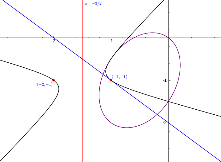
If 𝒪S​(−E−F)∈𝒜{\mathcal{O}}_{S}(-E-F)\in{\mathcal{A}}, then it could only be destabilized by 𝒪S​(−2​E−F){\mathcal{O}}_{S}(-2E-F). The wall 𝒲⁡(𝒪S​(−2​E−F),𝒪S​(−E−F)){\mathcal{W}}({\mathcal{O}}_{S}(-2E-F),{\mathcal{O}}_{S}(-E-F)) can be seen to be the same as the wall 𝒲⁡(𝒪S​(−E),𝒪S){\mathcal{W}}({\mathcal{O}}_{S}(-E),{\mathcal{O}}_{S}) moved one unit down and one unit to the left (see Figure 8). The right side of the hyperboloidal wall 𝒲⁡(𝒪S​(−2​E−F),𝒪S​(−E−F)){\mathcal{W}}({\mathcal{O}}_{S}(-2E-F),{\mathcal{O}}_{S}(-E-F)) is in the region where 𝒪S​(−E−F)∉𝒜{\mathcal{O}}_{S}(-E-F)\not\in{\mathcal{A}}, so we do not have to worry about it in this case. The left side of the wall is not in our region RR. Indeed, it can easily be checked that the two walls 𝒲⁡(𝒪S​(−2​E−F),𝒪S​(−E−F)){\mathcal{W}}({\mathcal{O}}_{S}(-2E-F),{\mathcal{O}}_{S}(-E-F)) and 𝒲⁡(𝒪S​(−E),𝒪S){\mathcal{W}}({\mathcal{O}}_{S}(-E),{\mathcal{O}}_{S}) do not cross the x=−3/2x=-3/2 vertical plane. The left side of the hyperboloid 𝒲⁡(𝒪S​(−2​E−F),𝒪S​(−E−F)){\mathcal{W}}({\mathcal{O}}_{S}(-2E-F),{\mathcal{O}}_{S}(-E-F)) is to the left of it, while the ellipsoid 𝒲⁡(𝒪S​(−E),𝒪S){\mathcal{W}}({\mathcal{O}}_{S}(-E),{\mathcal{O}}_{S}) is to the right of it (see Figure 8).

Refer to caption
Figure 8: The walls 𝒲⁡(𝒪S​(−2​E−F),𝒪S​(−E−F)){\mathcal{W}}({\mathcal{O}}_{S}(-2E-F),{\mathcal{O}}_{S}(-E-F)) and 𝒲⁡(𝒪S​(−E),𝒪S){\mathcal{W}}({\mathcal{O}}_{S}(-E),{\mathcal{O}}_{S}).

If, on the other hand, 𝒪S​(−E−F)​[1]∈𝒜{\mathcal{O}}_{S}(-E-F)[1]\in{\mathcal{A}}, then it could only be destabilized by the quotient 𝒪S​(−F)​[1]{\mathcal{O}}_{S}(-F)[1]. However, a quick calculation shows that the wall 𝒲⁡(𝒪S​(−E−F)​[1],𝒪S​(−F)​[1]){\mathcal{W}}({\mathcal{O}}_{S}(-E-F)[1],{\mathcal{O}}_{S}(-F)[1]) is equal to the wall 𝒲⁡(𝒪S​(−E−F)​[1],𝒪S​(E)|E){\mathcal{W}}({\mathcal{O}}_{S}(-E-F)[1],{{\mathcal{O}}_{S}(E)|_{E}}), and we already saw that such wall lies outside of our region RR when we look in the region where 𝒪S​(−E−F)​[1]∈𝒜{\mathcal{O}}_{S}(-E-F)[1]\in{\mathcal{A}} (see Figure 6).

Thus all objects of 𝔽′{\mathbb{F}}^{\prime} are σ\sigma-stable for σ∈R\sigma\in R and we have shown that R=R𝔽′R=R_{{\mathbb{F}}^{\prime}}, the quiver region associated to 𝔽′{\mathbb{F}}^{\prime}. ∎

The translations of R𝔽′R_{{\mathbb{F}}^{\prime}} by tensoring with line bundles do not cover the entire x​yxy-plane. We now find the quiver region associated to 𝔽′′{\mathbb{F}}^{\prime\prime} and show that the translations of both quiver regions together cover the x​yxy-plane.

5.4 Quiver region for 𝔼′′{\mathbb{E}}^{\prime\prime} and the combined regions

Determining the quiver region R𝔽′′R_{{\mathbb{F}}^{\prime\prime}} associated to

𝔼′′=(𝒪S,𝒪S​(E),G2,𝒪S​(E+F)){\mathbb{E}}^{\prime\prime}=({\mathcal{O}}_{S},\ {\mathcal{O}}_{S}(E),\ G_{2},\ {\mathcal{O}}_{S}(E+F))

and its dual collection

𝔽′′=(𝒪S​(−E−2​F)​[2],𝒪S​(−F)​[1],𝒪S​(E)|E,𝒪S){\mathbb{F}}^{\prime\prime}=({\mathcal{O}}_{S}(-E-2F)[2],\ {\mathcal{O}}_{S}(-F)[1],\ {{\mathcal{O}}_{S}(E)|_{E}},\ {\mathcal{O}}_{S})

is very similar to the determination of the region ℝ𝔽′{\mathbb{R}}_{{\mathbb{F}}^{\prime}}. Therefore, we summarize the argument and omit the details:

To have σ∈R𝔽′′\sigma\in R_{{\mathbb{F}}^{\prime\prime}} we must have

  • •

    𝒪S,𝒪S​(E)|E,𝒪S​(−E−2​F)​[1]∈𝒜{\mathcal{O}}_{S},{{\mathcal{O}}_{S}(E)|_{E}},{\mathcal{O}}_{S}(-E-2F)[1]\in{\mathcal{A}}

  • •

    β⁡(𝒪S),β⁡(𝒪S​(E)|E)>β⁡(𝒪S​(−E−2​F)​[1])\beta({\mathcal{O}}_{S}),\beta({{\mathcal{O}}_{S}(E)|_{E}})>\beta({\mathcal{O}}_{S}(-E-2F)[1]).

Moreover, one of the following two things must happen:

  • •

    𝒪S​(−F)∈𝒜{\mathcal{O}}_{S}(-F)\in{\mathcal{A}}, and β⁡(𝒪S),β⁡(𝒪S​(E)|E)>β⁡(𝒪S​(−F))\beta({\mathcal{O}}_{S}),\beta({{\mathcal{O}}_{S}(E)|_{E}})>\beta({\mathcal{O}}_{S}(-F)), or

  • •

    𝒪S​(−F)​[1]∈𝒜{\mathcal{O}}_{S}(-F)[1]\in{\mathcal{A}}, and β⁡(𝒪S​(−F)​[1])>β⁡(𝒪S​(−E−2​F)​[1])\beta({\mathcal{O}}_{S}(-F)[1])>\beta({\mathcal{O}}_{S}(-E-2F)[1]).

Also, all objects of 𝔽′′{\mathbb{F}}^{\prime\prime} must also be σ\sigma-stable.

Any σ\sigma satisfying the above is a quiver stability condition, and we find that ℝ𝔽′′{\mathbb{R}}_{{\mathbb{F}}^{\prime\prime}} is the region strictly inside both the ellipsoidal wall 𝒲⁡(𝒪S,𝒪S​(−E−2​F)​[1]){\mathcal{W}}({\mathcal{O}}_{S},{\mathcal{O}}_{S}(-E-2F)[1]) and the hyperboloidal wall 𝒲⁡(𝒪S​(E)|E,𝒪S​(−E−2​F)​[1]){\mathcal{W}}({{\mathcal{O}}_{S}(E)|_{E}},{\mathcal{O}}_{S}(-E-2F)[1]). Figure 9 shows the intersection of these walls with the x​yxy-plane, as well as the lines that determine if 𝒪S,𝒪S​(−E−2​F)​[1]∈𝒜{\mathcal{O}}_{S},{\mathcal{O}}_{S}(-E-2F)[1]\in{\mathcal{A}}.

Refer to caption
Figure 9: The ellipsoidal wall 𝒲⁡(𝒪S,𝒪S​(−E−2​F)​[1]){\mathcal{W}}({\mathcal{O}}_{S},{\mathcal{O}}_{S}(-E-2F)[1]) and the hyperboloidal wall 𝒲⁡(𝒪S​(E)|E,𝒪S​(−E−2​F)​[1]){\mathcal{W}}({{\mathcal{O}}_{S}(E)|_{E}},{\mathcal{O}}_{S}(-E-2F)[1]).

The projection of the union of the two quiver regions R𝔽′∪R𝔽′′R_{{\mathbb{F}}^{\prime}}\cup R_{{\mathbb{F}}^{\prime\prime}} to the x​yxy-plane is the region strictly bounded by the ellipse that is the intersection of 𝒲⁡(𝒪S,𝒪S​(−E−2​F)​[1]){\mathcal{W}}({\mathcal{O}}_{S},{\mathcal{O}}_{S}(-E-2F)[1]) with the x​yxy-plane. Indeed, the two hyperboloidal walls 𝒲⁡(𝒪S,𝒪S​(E)|E){\mathcal{W}}({\mathcal{O}}_{S},{{\mathcal{O}}_{S}(E)|_{E}}) and 𝒲⁡(𝒪S​(E)|E,𝒪S​(−E−2​F)​[1]){\mathcal{W}}({{\mathcal{O}}_{S}(E)|_{E}},{\mathcal{O}}_{S}(-E-2F)[1]) overlap, as in Figure 10.

Refer to caption
Figure 10: The projection of the quiver regions R𝔽′R_{{\mathbb{F}}^{\prime}} and R𝔽′′R_{{\mathbb{F}}^{\prime\prime}} is the region strictly bounded by the ellipse 𝒲⁡(𝒪S,𝒪S​(−E−2​F)​[1]){\mathcal{W}}({\mathcal{O}}_{S},{\mathcal{O}}_{S}(-E-2F)[1]).

The ellipse bounds a parallelogram with two corners cut off:

U={(x,y)|−1≤x≤0,x−1≤y≤x}∖{(0,0),(−1,−2)}.U=\{(x,y)|-1\leq x\leq 0,\ x-1\leq y\leq x\}\smallsetminus\{(0,0),(-1,-2)\}.

The analogous region U⁡(p,q)U(p,q) associated to the quiver regions R𝔽′⊗𝒪S​(p,q)R_{{\mathbb{F}}^{\prime}\otimes{\mathcal{O}}_{S}(p,q)} and R𝔽′′⊗𝒪S​(p,q)R_{{\mathbb{F}}^{\prime\prime}\otimes{\mathcal{O}}_{S}(p,q)} is U+(p,q)U+(p,q), where the ++ indicates component-wise addition, and together the regions U⁡(p,q)U(p,q) cover the entire x​yxy-plane. Recalling the argument given in Section 3, we have shown the following.

Proposition 5.4.

Conjecture 1 holds for S=B​lp​ℙ2S=Bl_{p}{\mathbb{P}}^{2}. In particular, if the invariants vv satisfy the Bogomolov inequality, then every moduli space ℳσ​(v){\mathcal{M}}_{\sigma}(v) is isomorphic to a moduli space ℳσ′​(v){\mathcal{M}}_{\sigma^{\prime}}(v) where σ′\sigma^{\prime} is in a quiver region R𝔽′⊗𝒪S​(p,q)R_{{\mathbb{F}}^{\prime}\otimes{\mathcal{O}}_{S}(p,q)} or R𝔽′′⊗𝒪S​(p,q)R_{{\mathbb{F}}^{\prime\prime}\otimes{\mathcal{O}}_{S}(p,q)}, and hence ℳσ​(v){\mathcal{M}}_{\sigma}(v) is projective.

Appendix A Mutations defined by height functions

Here we give the precise definition of a mutation defined by a height function for an object E⋆E_{\star} in an exceptional collection or helix. We first address a few preliminaries before the definition then show that the information necessary to perform a mutation defined by a height function is contained in the quiver associated to a particular thread of the helix. We recall the definitions given in Section 2.2, but for the sake of generality we now allow the surface SS to be a smooth, projective variety XX over ℂ{\mathbb{C}}.

Given an exceptional collection 𝔼{\mathbb{E}} of objects in D⁡(X)D(X), we define the right orthogonal category as the full subcategory 𝔼⟂={G∈D|Hom∙​(E⋆,G)=0​ for all ​E⋆∈𝔼}{\mathbb{E}}^{\perp}=\{G\in D\ |\ \text{Hom}^{\bullet}(E_{\star},G)=0\text{ for all }E_{\star}\in{\mathbb{E}}\}. The left orthogonal category ⟂𝔼{}^{\perp}{\mathbb{E}} is defined similarly. For E⋆E_{\star} an exceptional object and G∈⟂E⋆G\in{}^{\perp}E_{\star}, the left mutation1010 10 Dually, we may define a right mutation. of GG through E⋆E_{\star}, LE⋆​(G)L_{E_{\star}}(G), is defined by the canonical evaluation triangle

Hom∙​(E⋆,G)⊗E⋆→G→LE⋆​(G).\text{Hom}^{\bullet}(E_{\star},G)\otimes E_{\star}\rightarrow G\rightarrow L_{E_{\star}}(G).

Note that LE⋆​(G)∈E⋆⟂L_{E_{\star}}(G)\in E_{\star}^{\perp}. If 𝔼=(E1,…,Ek){\mathbb{E}}=(E_{1},\ldots,E_{k}) we will denote LE1LE2⋯LEkGL_{E_{1}}L_{E_{2}}\cdots L_{E_{k}}G by L𝔼​(G)L_{{\mathbb{E}}}(G).

Let 𝔼=(E1,…,En){\mathbb{E}}=(E_{1},\ldots,E_{n}) be a full strong exceptional collection of objects in D⁡(X)D(X) with dual collection 𝔽=(Fn,…,F1){\mathbb{F}}=(F_{n},\ldots,F_{1}). Bridgeland and Stern [BS10] define the notion of pp-related, which is crucial to that of height functions: if i<ji<j we say that EiE_{i} and EjE_{j} are pp-related if Homk​(Fj,Fi)=0\text{Hom}^{k}(F_{j},F_{i})=0 for k≠pk\neq p.

A height function for an object E⋆∈𝔼E_{\star}\in{\mathbb{E}} is a function (called a“levelling”) ϕ:𝔼→ℤ\phi:{\mathbb{E}}\rightarrow{\mathbb{Z}} such that ϕ−1​(0)={E⋆}\phi^{-1}(0)=\{E_{\star}\}, and ϕ⁡(Ej)=p≠0\phi(E_{j})=p\neq 0 implies that EE and EjE_{j} are pp-related if p≥0p\geq 0, or if p<0p<0 then EjE_{j} and EE are −p-p-related. One defines height functions for helices be asking ϕ⁡(Ei+n)=ϕ⁡(Ei)+1+dimX\phi(E_{i+n})=\phi(E_{i})+1+\dim X for each ii and the above pp-related conditions to hold for any thread in the helix.

Given a geometric helix ℍ=(Ei)i∈ℤ{\mathbb{H}}=(E_{i})_{i\in{\mathbb{Z}}} with a height function ϕ\phi for E⋆E_{\star}, a mutation defined by a height function for E⋆E_{\star} (henceforth called a left tilt at E⋆E_{\star}) constructs a related helix and levelling. We describe the operation algorithmically: to perform a left tilt at E⋆E_{\star}…

  • •

    Choose a thread 𝔼=(Ek,…,Ek+n){\mathbb{E}}=(E_{k},\ldots,E_{k+n}) of ℍ{\mathbb{H}} which contains both E⋆E_{\star} and ϕ−1​(−1)=:𝔼−1\phi^{-1}(-1)=:{\mathbb{E}}_{-1}, i.e where 𝔼=(…,𝔼−1,E⋆,…){\mathbb{E}}=(\ldots,{\mathbb{E}}_{-1},E_{\star},\ldots).

  • •

    Left mutate (and shift) EE through 𝔼−1{\mathbb{E}}_{-1} and keep this new positioning, i.e. 𝔼′=(…,L𝔼−1​E⋆​[−1],𝔼−1,…){\mathbb{E}}^{\prime}=(\ldots,L_{{\mathbb{E}}_{-1}}E_{\star}[-1],{\mathbb{E}}_{-1},\ldots).

  • •

    Use 𝔼′{\mathbb{E}}^{\prime} to generate a helix ℍ′{\mathbb{H}}^{\prime} and a levelling ϕ′\phi^{\prime} such that ϕ′−1​(−1)=L𝔼−1​E⋆​[−1]\phi^{\prime-1}(-1)=L_{{\mathbb{E}}_{-1}}E_{\star}[-1] and ϕ′−1​(0)=𝔼−1\phi^{\prime-1}(0)={\mathbb{E}}_{-1}.

  • •

    The pair (OPENℍ′,ϕ′)=:σ0​(ℍ,ϕ){\mathbb{H}}^{\prime},\phi^{\prime})=:\sigma_{0}({\mathbb{H}},\phi) is the result of the left tilt at E⋆E_{\star}.

Recall (Section 2.2) that to a full strong exceptional collection we associate a quiver where the number of arrows from vertex ii to vertex jj is ni​j=dimHom1​(Fj,Fi)n_{ij}=\dim\text{Hom}^{1}(F_{j},F_{i}). We claim that the helix ℍ′{\mathbb{H}}^{\prime} obtained via a left tilt at E⋆E_{\star} can be deduced using the the quiver associated to the thread 𝔼=(E1,…,En=E⋆){\mathbb{E}}=(E_{1},\ldots,E_{n}=E_{\star})1111 11 Note that we may always harmlessly change the indexing of ℍ{\mathbb{H}} so that E⋆=EnE_{\star}=E_{n}.. The idea is that, if EiE_{i}’s vertex has an arrow to E⋆E_{\star}’s vertex, then dimHom1​(Fn,Fi)>0\dim\text{Hom}^{1}(F_{n},F_{i})>0 and it will follow that EiE_{i} and E⋆E_{\star} are 1-related and hence Ei∈𝔼−1E_{i}\in{\mathbb{E}}_{-1}. The essence of Proposition A.1 is that the other objects in 𝔼−1{\mathbb{E}}_{-1} do not meaningfully affect the result of the mutation.

Proposition A.1.

Let ℍ{\mathbb{H}} be a geometric helix of exceptional objects of D⁡(X)D(X) and let ϕ\phi be a height function for E⋆∈ℍE_{\star}\in{\mathbb{H}}. Consider the thread 𝔼=(E1,…,En=E⋆){\mathbb{E}}=(E_{1},\ldots,E_{n}=E_{\star}) and set

𝔼−1a:={objects in 𝔼 whose vertex has arrows to E⋆’s vertex}.{\mathbb{E}}_{-1}^{a}:=\{\text{objects in ${\mathbb{E}}$ whose vertex has arrows to $E_{\star}$'s vertex}\}.

Then the helix ℍ′{\mathbb{H}}^{\prime} obtained through a left tilt at E⋆E_{\star} is obtained by taking E⋆E_{\star}, moving it just to the left of the last object of 𝔼−1a{\mathbb{E}}_{-1}^{a}, then replacing E⋆E_{\star} with L𝔼−1a​(E⋆)​[−1]L_{{\mathbb{E}}_{-1}^{a}}(E_{\star})[-1] and generating the helix1212 12 We speak algorithmically to avoid cumbersome notation. For instance, a priori there may be objects between E⋆E_{\star} and those of 𝔼−1a{\mathbb{E}}_{-1}^{a}..

Remark.

We identify two helices if they differ by a rearrangement of mutually orthogonal, adjacent objects. Since AA mutually orthogonal to BB implies that LA​B=BL_{A}B=B, it follows that the objects of the dual collection 𝔽{\mathbb{F}} do not change after shuffling mutually orthogonal objects of a thread 𝔼{\mathbb{E}}.

Proof of Proposition A.1.

To left tilt ℍ{\mathbb{H}} at E⋆E_{\star}, one takes E⋆E_{\star}, moves it just to the left of 𝔼−1{\mathbb{E}}_{-1} and then replaces E⋆E_{\star} with L𝔼−1​(E⋆)​[−1]L_{{\mathbb{E}}_{-1}}(E_{\star})[-1]. We show that our process produces the same result.

To begin, in the proof of [BS10, Proposition 7.1] (using m=0,k=1,i=nm=0,k=1,i=n), we may replace 𝔼−1{\mathbb{E}}_{-1} with 𝔼−1a{\mathbb{E}}_{-1}^{a}, since if EjE_{j} has no arrows to E⋆E_{\star} then dj​n1:=dim Hom1​(Fn,Fj)=0d^{1}_{jn}:=\text{dim }\text{Hom}^{1}(F_{n},F_{j})=0. It follows that L𝔼−1​(E⋆)≅L𝔼−1a​(E⋆)=:ℒL_{{\mathbb{E}}_{-1}}(E_{\star})\cong L_{{\mathbb{E}}_{-1}^{a}}(E_{\star})=:{\mathcal{L}}. Furthermore, it follows from [BS10, Proposition 7.1] that for any two height functions ϕ,ϕ~\phi,\widetilde{\phi} for E⋆E_{\star} we have L𝔼−1​(E⋆)≅L𝔼~−1​(E⋆)L_{{\mathbb{E}}_{-1}}(E_{\star})\cong L_{\widetilde{{\mathbb{E}}}_{-1}}(E_{\star}).

Call the sequence our process produces ℍa{\mathbb{H}}^{a}. We show that ℍa{\mathbb{H}}^{a} is obtained by a left tilt at E⋆E_{\star} by adjusting the height function ϕ\phi to obtain a new height function ϕ~\widetilde{\phi}, where the left-most object of L𝔼~−1​(E)L_{\widetilde{{\mathbb{E}}}_{-1}}(E) is the left-most object in 𝔼−1a{\mathbb{E}}_{-1}^{a}. It follows that ℍa{\mathbb{H}}^{a} is a geometric helix. We then show that ℍa{\mathbb{H}}^{a} differs from ℍ′{\mathbb{H}}^{\prime} by moving ℒ{\mathcal{L}} across a (possibly empty) set of objects with which it is mutually orthogonal.

Let 𝔽=(Fn,…,F1){\mathbb{F}}=(F_{n},\ldots,F_{1}) be the dual collection corresponding to 𝔼{\mathbb{E}}. Since the height function ϕ\phi exists by assumption, if Homp​(Fn,Fi)≠0\text{Hom}^{p}(F_{n},F_{i})\neq 0 for some pp, then pp is the only such degree. Now, suppose Ei∈𝔼−1E_{i}\in{\mathbb{E}}_{-1}. Then either dimHom1​(Fn,Fi)≠0\dim\text{Hom}^{1}(F_{n},F_{i})\neq 0 (and thus EiE_{i}’s vertex has an arrow to E⋆E_{\star}’s vertex) or dimHomp​(Fn,Fi)=0\dim\text{Hom}^{p}(F_{n},F_{i})=0 for all pp (in which case there are no arrows from EiE_{i}’s vertex to E⋆E_{\star}’s vertex).

By definition, 𝔼−1a{\mathbb{E}}_{-1}^{a} is the subset of 𝔼{\mathbb{E}} with dimHom1​(F0,Fi)≠0\dim\text{Hom}^{1}(F_{0},F_{i})\neq 0 and thus 𝔼−1a⊂𝔼−1{\mathbb{E}}_{-1}^{a}\subset{\mathbb{E}}_{-1}. It follows that any object EjE_{j} of 𝔼−1{\mathbb{E}}_{-1} that is to the left of 𝔼−1a{\mathbb{E}}_{-1}^{a} (in the ordering of 𝔼{\mathbb{E}}) has Homp​(Fn,Fj)=0\text{Hom}^{p}(F_{n},F_{j})=0 for all pp and so can be moved into 𝔼−2{\mathbb{E}}_{-2}. Doing this gives a height function ϕ~\widetilde{\phi}, where a left tilt at E⋆E_{\star} is accomplished by moving E⋆E_{\star} just to the left of 𝔼~−1\widetilde{{\mathbb{E}}}_{-1} (which is the same as just to the left of 𝔼−1a{\mathbb{E}}_{-1}^{a}) and replacing E⋆E_{\star} with L𝔼~−1​(E⋆)≅L𝔼−1​(E⋆)≅ℒL_{\widetilde{{\mathbb{E}}}_{-1}}(E_{\star})\cong L_{{\mathbb{E}}_{-1}}(E_{\star})\cong{\mathcal{L}}.

Since placing ℒ{\mathcal{L}} either to the left of 𝔼−1{\mathbb{E}}_{-1} or to the left of 𝔼−1a{\mathbb{E}}_{-1}^{a} gives a geometric helix, we conclude that ℒ{\mathcal{L}} is mutually orthogonal to all objects that are in 𝔼−1{\mathbb{E}}_{-1} but to the left of 𝔼−1a{\mathbb{E}}_{-1}^{a}. ∎

Appendix B Calculations

B.1 χ⁡(A,B)\chi(A,B) in ℙ1×ℙ1{\mathbb{P}}^{1}\times{\mathbb{P}}^{1}

Let A,BA,B be two objects of rank rA,rBr_{A},r_{B}, respectively. Suppose moreover that c1​(A)=a1​D1+a2​D2c_{1}(A)=a_{1}D_{1}+a_{2}D_{2} and c1​(B)=b1​D1+b2​D2c_{1}(B)=b_{1}D_{1}+b_{2}D_{2}. Then,

χ⁡(A,B)=rA​rB+12​(rA​dB−rB​dA)+rB​ch2​(A)+rA​ch2​(B)−c1​(A)​c1​(B),\chi(A,B)=r_{A}r_{B}+\frac{1}{2}(r_{A}d_{B}-r_{B}d_{A})+r_{B}{\textrm{ch}}_{2}(A)+r_{A}{\textrm{ch}}_{2}(B)-c_{1}(A)c_{1}(B),

where dAd_{A} (resp. dBd_{B}) is the degree of AA (resp. BB) defined by dA=−KS⋅c1(A)d_{A}=-K_{S}\cdot c_{1}(A) (resp. dB=−KS⋅c1(B)d_{B}=-K_{S}\cdot c_{1}(B)). Since KS=−2​D1−2​D2K_{S}=-2D_{1}-2D_{2}, we have that dA=2​(a1+a2)d_{A}=2(a_{1}+a_{2}) (resp. dB=2​(b1+b2)d_{B}=2(b_{1}+b_{2})), and

χ⁡(A,B)=rA​rB+rA​(b1+b2)−rB​(a1+a2)+rB​ch2​(A)+rA​ch2​(B)−c1​(A)​c1​(B).\chi(A,B)=r_{A}r_{B}+r_{A}(b_{1}+b_{2})-r_{B}(a_{1}+a_{2})+r_{B}{\textrm{ch}}_{2}(A)+r_{A}{\textrm{ch}}_{2}(B)-c_{1}(A)c_{1}(B).

B.2 L𝒪S​(1,0)​L𝒪S​(0,1)​(𝒪S​(1,1))L_{{\mathcal{O}}_{S}(1,0)}L_{{\mathcal{O}}_{S}(0,1)}({\mathcal{O}}_{S}(1,1)) in ℙ1×ℙ1{\mathbb{P}}^{1}\times{\mathbb{P}}^{1}

  • •

    To calculate L𝒪S​(0,1)​(𝒪S​(1,1))L_{{\mathcal{O}}_{S}(0,1)}({\mathcal{O}}_{S}(1,1)), note that

    χ⁡(𝒪S​(0,1),𝒪S​(1,1))=1+2−1+1−1=2.\chi({\mathcal{O}}_{S}(0,1),{\mathcal{O}}_{S}(1,1))=1+2-1+1-1=2.

    Therefore, we obtain the map

    𝒪S​(0,1)⊕2⟶𝒪S​(1,1),{\mathcal{O}}_{S}(0,1)^{\oplus 2}\longrightarrow{\mathcal{O}}_{S}(1,1),

    and L𝒪S​(0,1)​(𝒪S​(1,1))=𝒪S​(−1,1)​[1]L_{{\mathcal{O}}_{S}(0,1)}({\mathcal{O}}_{S}(1,1))={\mathcal{O}}_{S}(-1,1)[1].

    • –

      To calculate L𝒪S​(1,0)​(𝒪S​(−1,1)​[1])L_{{\mathcal{O}}_{S}(1,0)}({\mathcal{O}}_{S}(-1,1)[1]), note that

      χ⁡(𝒪S​(1,0),𝒪S​(−1,1))=1−1−1−1=−2.\chi({\mathcal{O}}_{S}(1,0),{\mathcal{O}}_{S}(-1,1))=1-1-1-1=-2.

      Therefore, we obtain the map

      𝒪S​(1,0)⊕2⟶𝒪S​(−1,1)​[1],{\mathcal{O}}_{S}(1,0)^{\oplus 2}\longrightarrow{\mathcal{O}}_{S}(-1,1)[1],

      and L𝒪S​(1,0)​(𝒪S​(−1,1)​[1])=G⁡[1]L_{{\mathcal{O}}_{S}(1,0)}({\mathcal{O}}_{S}(-1,1)[1])=G[1], where GG is a rank 3 extension of 𝒪S​(1,0)⊕2{\mathcal{O}}_{S}(1,0)^{\oplus 2} by 𝒪S​(−1,1){\mathcal{O}}_{S}(-1,1). We have that rk​(G)=3{\textrm{rk}}(G)=3, c1​(G)=D1+D2c_{1}(G)=D_{1}+D_{2}, and ch2​(G)=−1{\textrm{ch}}_{2}(G)=-1.

B.3 𝔽′{\mathbb{F}}^{\prime} in ℙ1×ℙ1{\mathbb{P}}^{1}\times{\mathbb{P}}^{1}

Recall that

𝔼′=(𝒪S,G,𝒪S​(1,0),𝒪S​(0,1)),{\mathbb{E}}^{\prime}=({\mathcal{O}}_{S},G,{\mathcal{O}}_{S}(1,0),{\mathcal{O}}_{S}(0,1)),

where GG is a sheaf of rank 3 with c1​(G)=D1+D2c_{1}(G)=D_{1}+D_{2} and ch2​(G)=−1{\textrm{ch}}_{2}(G)=-1.

We calculate here the dual collection 𝔽′{\mathbb{F}}^{\prime}.

  • •

    To calculate L𝒪S​(G)L_{{\mathcal{O}}_{S}}(G), note that

    χ⁡(𝒪S,G)=3+2−1=4.\chi({\mathcal{O}}_{S},G)=3+2-1=4.

    Therefore, we obtain the map

    𝒪S⊕4⟶G,{\mathcal{O}}_{S}^{\oplus 4}\longrightarrow G,

    and L𝒪S​(G)=𝒪S​(−1,−1)​[1]L_{{\mathcal{O}}_{S}}(G)={\mathcal{O}}_{S}(-1,-1)[1].

  • •

    To calculate LG​(𝒪S​(1,0))L_{G}({\mathcal{O}}_{S}(1,0)), note that

    χ⁡(G,𝒪S​(1,0))=3+3−2−1−1=2.\chi(G,{\mathcal{O}}_{S}(1,0))=3+3-2-1-1=2.

    Therefore, we obtain the map

    G⊕2⟶𝒪S​(1,0),G^{\oplus 2}\longrightarrow{\mathcal{O}}_{S}(1,0),

    and LG​(𝒪S​(1,0))=G1​[1]L_{G}({\mathcal{O}}_{S}(1,0))=G_{1}[1], where G1G_{1} has rk​(G1)=5{\textrm{rk}}(G_{1})=5, c1​(G1)=D1+2​D2c_{1}(G_{1})=D_{1}+2D_{2}, and ch2​(G1)=−2{\textrm{ch}}_{2}(G_{1})=-2.

    • –

      To calculate L𝒪S​(G1​[1])L_{{\mathcal{O}}_{S}}(G_{1}[1]), note that

      χ⁡(𝒪S,G1)=5+3−2=6.\chi({\mathcal{O}}_{S},G_{1})=5+3-2=6.

      Therefore, we obtain the map

      𝒪S⊕6​[1]⟶G1​[1],{\mathcal{O}}_{S}^{\oplus 6}[1]\longrightarrow G_{1}[1],

      and L𝒪S​(G1​[1])=𝒪S​(−1,−2)​[2]L_{{\mathcal{O}}_{S}}(G_{1}[1])={\mathcal{O}}_{S}(-1,-2)[2].

  • •

    We may calculate L𝒪S​LG​L𝒪S​(1,0)​(𝒪S​(0,1))L_{{\mathcal{O}}_{S}}L_{G}L_{{\mathcal{O}}_{S}(1,0)}({\mathcal{O}}_{S}(0,1)) with similar computations, but it is faster to use [BS10, Corollary 2.10 & Definition 3.1] to obtain

    L𝒪S​LG​L𝒪S​(1,0)​(𝒪S​(0,1))=𝒪S​(0,1)⊗ωS​[2]=𝒪S​(−2,−1)​[2].L_{{\mathcal{O}}_{S}}L_{G}L_{{\mathcal{O}}_{S}(1,0)}({\mathcal{O}}_{S}(0,1))={\mathcal{O}}_{S}(0,1)\otimes\omega_{S}[2]={\mathcal{O}}_{S}(-2,-1)[2].

Therefore,

𝔽′=(𝒪S​(−2,−1)​[2],𝒪S​(−1,−2)​[2],𝒪S​(−1,−1)​[1],𝒪S).{\mathbb{F}}^{\prime}=({\mathcal{O}}_{S}(-2,-1)[2],{\mathcal{O}}_{S}(-1,-2)[2],{\mathcal{O}}_{S}(-1,-1)[1],{\mathcal{O}}_{S}).

B.4 χ⁡(A,B)\chi(A,B) in B​lp​ℙ2Bl_{p}{\mathbb{P}}^{2}

Let A,BA,B be two objects of rank rA,rBr_{A},r_{B}, respectively. Suppose moreover that c1​(A)=aE​E+aF​Fc_{1}(A)=a_{E}E+a_{F}F and c1​(B)=bE​E+bF​Fc_{1}(B)=b_{E}E+b_{F}F. Then,

χ⁡(A,B)=rA​rB+12​(rA​dB−rB​dA)+rB​ch2​(A)+rA​ch2​(B)−c1​(A)​c1​(B),\chi(A,B)=r_{A}r_{B}+\frac{1}{2}(r_{A}d_{B}-r_{B}d_{A})+r_{B}{\textrm{ch}}_{2}(A)+r_{A}{\textrm{ch}}_{2}(B)-c_{1}(A)c_{1}(B),

where dAd_{A} (resp. dBd_{B}) is the degree of AA (resp. BB) defined by dA=−KS⋅c1(A)d_{A}=-K_{S}\cdot c_{1}(A) (resp. dB=−KS⋅c1(B)d_{B}=-K_{S}\cdot c_{1}(B)). Since KS=−3​H+E=−2​E−3​FK_{S}=-3H+E=-2E-3F, we have that dA=aE+2​aFd_{A}=a_{E}+2a_{F} (resp. dB=bE+2​bFd_{B}=b_{E}+2b_{F}).

In particular,

χ⁡(𝒪S,B)=rB+12​bE+bF+ch2​(B).\chi({\mathcal{O}}_{S},B)=r_{B}+\frac{1}{2}b_{E}+b_{F}+{\textrm{ch}}_{2}(B).

If BB is a line bundle LL, then rB=1r_{B}=1 and ch2​(B)=(c1​(B))2/2=bE​bF−bE2/2{\textrm{ch}}_{2}(B)=(c_{1}(B))^{2}/2=b_{E}b_{F}-b_{E}^{2}/2, so we would have

χ⁡(𝒪S,L)=1+12​(bE−bE2)+bF+bE​bF.\chi({\mathcal{O}}_{S},L)=1+\frac{1}{2}(b_{E}-b_{E}^{2})+b_{F}+b_{E}b_{F}.

B.5 L𝒪S​(F)​L𝒪S​(E+F)​(𝒪S​(E+2​F))L_{{\mathcal{O}}_{S}(F)}L_{{\mathcal{O}}_{S}(E+F)}({\mathcal{O}}_{S}(E+2F)) in B​lp​ℙ2Bl_{p}{\mathbb{P}}^{2}

  • •

    To calculate L𝒪S​(E+F)​(𝒪S​(E+2​F))L_{{\mathcal{O}}_{S}(E+F)}({\mathcal{O}}_{S}(E+2F)), note that

    χ⁡(𝒪S​(E+F),𝒪S​(E+2​F))=1+12​(5−3)+12+32−2=2.\chi({\mathcal{O}}_{S}(E+F),{\mathcal{O}}_{S}(E+2F))=1+\frac{1}{2}(5-3)+\frac{1}{2}+\frac{3}{2}-2=2.

    Therefore, we obtain the map

    𝒪S​(E+F)⊕2⟶𝒪S​(E+2​F),{\mathcal{O}}_{S}(E+F)^{\oplus 2}\longrightarrow{\mathcal{O}}_{S}(E+2F),

    and L𝒪S​(E+F)​(𝒪S​(E+2​F))=𝒪S​(E)​[1]L_{{\mathcal{O}}_{S}(E+F)}({\mathcal{O}}_{S}(E+2F))={\mathcal{O}}_{S}(E)[1].

    • –

      To calculate L𝒪S​(F)​(𝒪S​(E)​[1])L_{{\mathcal{O}}_{S}(F)}({\mathcal{O}}_{S}(E)[1]), note that

      χ⁡(𝒪S​(F),𝒪S​(E))=1+12​(1−2)+0−12−1=−1.\chi({\mathcal{O}}_{S}(F),{\mathcal{O}}_{S}(E))=1+\frac{1}{2}(1-2)+0-\frac{1}{2}-1=-1.

      Therefore, we obtain the map

      𝒪S​(F)⟶𝒪S​(E)​[1],{\mathcal{O}}_{S}(F)\longrightarrow{\mathcal{O}}_{S}(E)[1],

      and L𝒪S​(F)​(𝒪S​(E)​[1])=G1​[1]L_{{\mathcal{O}}_{S}(F)}({\mathcal{O}}_{S}(E)[1])=G_{1}[1], where G1G_{1} is the rank 2 extension of 𝒪S​(F){\mathcal{O}}_{S}(F) by 𝒪S​(E){\mathcal{O}}_{S}(E). We have that rk​(G1)=2{\textrm{rk}}(G_{1})=2, c1​(G1)=E+Fc_{1}(G_{1})=E+F, and ch2(G1)=−1/2{\textrm{ch}}_{2}(G_{1})=-1/2.

B.6 𝔽′{\mathbb{F}}^{\prime} in B​lp​ℙ2Bl_{p}{\mathbb{P}}^{2}

Recall that

𝔼′=(𝒪S,G1,𝒪S​(F),𝒪S​(E+F)),{\mathbb{E}}^{\prime}=({\mathcal{O}}_{S},G_{1},{\mathcal{O}}_{S}(F),{\mathcal{O}}_{S}(E+F)),

where G1G_{1} is a sheaf of rank 2 with c1​(G1)=E+Fc_{1}(G_{1})=E+F, and ch2(G1)=−1/2{\textrm{ch}}_{2}(G_{1})=-1/2. We calculate here the dual collection 𝔽′{\mathbb{F}}^{\prime}.

  • •

    To calculate L𝒪S​(G1)L_{{\mathcal{O}}_{S}}(G_{1}), note that

    χ⁡(𝒪S,G1)=2+12⋅3−12=3.\chi({\mathcal{O}}_{S},G_{1})=2+\frac{1}{2}\cdot 3-\frac{1}{2}=3.

    Therefore, we obtain the map

    𝒪S⊕3⟶G1,{\mathcal{O}}_{S}^{\oplus 3}\longrightarrow G_{1},

    and L𝒪S​(G1)=𝒪S​(−E−F)​[1]L_{{\mathcal{O}}_{S}}(G_{1})={\mathcal{O}}_{S}(-E-F)[1].

  • •

    To calculate LG1​(𝒪S​(F))L_{G_{1}}({\mathcal{O}}_{S}(F)), note that

    χ⁡(G1,𝒪S​(F))=2+12​(4−3)−12−1=1.\chi(G_{1},{\mathcal{O}}_{S}(F))=2+\frac{1}{2}(4-3)-\frac{1}{2}-1=1.

    Therefore, we obtain the map

    G1⟶𝒪S​(F),G_{1}\longrightarrow{\mathcal{O}}_{S}(F),

    and LG1​(𝒪S​(F))=𝒪S​(E)​[1]L_{G_{1}}({\mathcal{O}}_{S}(F))={\mathcal{O}}_{S}(E)[1].

    • –

      To calculate L𝒪S​(𝒪S​(E)​[1])L_{{\mathcal{O}}_{S}}({\mathcal{O}}_{S}(E)[1]), note that

      χ⁡(𝒪S,𝒪S​(E))=1+12−12=1.\chi({\mathcal{O}}_{S},{\mathcal{O}}_{S}(E))=1+\frac{1}{2}-\frac{1}{2}=1.

      Therefore, we obtain the map

      𝒪S​[1]⟶𝒪S​(E)​[1],{\mathcal{O}}_{S}[1]\longrightarrow{\mathcal{O}}_{S}(E)[1],

      and L𝒪S​(𝒪S​(E)​[1])=𝒪S​(E)|E​[1]L_{{\mathcal{O}}_{S}}({\mathcal{O}}_{S}(E)[1])={\mathcal{O}}_{S}(E)|_{E}[1]. Note that 𝒪S​(E)|E{\mathcal{O}}_{S}(E)|_{E} has rank 0, c1=Ec_{1}=E, and ch2=−1/2{\textrm{ch}}_{2}=-1/2. It is therefore isomorphic to 𝒪S​(−E−2​F)|E{\mathcal{O}}_{S}(-E-2F)|_{E}, which has the same invariants.

  • •

    Using [BS10, Corollary 2.10 & Definition 3.1], we calculate

    L𝒪S​LG1​L𝒪S​(F)​(𝒪S​(E+F))=𝒪S​(E+F)⊗ωS​[2]=𝒪S​(−E−2​F)​[2].L_{{\mathcal{O}}_{S}}L_{G_{1}}L_{{\mathcal{O}}_{S}(F)}({\mathcal{O}}_{S}(E+F))={\mathcal{O}}_{S}(E+F)\otimes\omega_{S}[2]={\mathcal{O}}_{S}(-E-2F)[2].

Therefore,

𝔽′=(𝒪S​(−E−2​F)​[2],𝒪S​(E)|E​[1],𝒪S​(−E−F)​[1],𝒪S).{\mathbb{F}}^{\prime}=({\mathcal{O}}_{S}(-E-2F)[2],{\mathcal{O}}_{S}(E)|_{E}[1],{\mathcal{O}}_{S}(-E-F)[1],{\mathcal{O}}_{S}).

B.7 L𝒪S​(E+F)​(𝒪S​(2​E+2​F))L_{{\mathcal{O}}_{S}(E+F)}({\mathcal{O}}_{S}(2E+2F)) in B​lp​ℙ2Bl_{p}{\mathbb{P}}^{2}

Note that

χ⁡(𝒪S​(E+F),𝒪S​(2​E+2​F))=1+12​(6−3)+12+2−2=3.\chi({\mathcal{O}}_{S}(E+F),{\mathcal{O}}_{S}(2E+2F))=1+\frac{1}{2}(6-3)+\frac{1}{2}+2-2=3.

Therefore, we obtain the map

𝒪S​(E+F)⊕3⟶𝒪S​(2​E+2​F),{\mathcal{O}}_{S}(E+F)^{\oplus 3}\longrightarrow{\mathcal{O}}_{S}(2E+2F),

and L𝒪S​(E+F)​(𝒪S​(E+2​F))=G2​[1]L_{{\mathcal{O}}_{S}(E+F)}({\mathcal{O}}_{S}(E+2F))=G_{2}[1], where G2G_{2} is a sheaf with rk​(G2)=2{\textrm{rk}}(G_{2})=2, c1​(G2)=E+Fc_{1}(G_{2})=E+F, and ch2(G2)=−1/2{\textrm{ch}}_{2}(G_{2})=-1/2.

B.8 𝔽′′{\mathbb{F}}^{\prime\prime} in B​lp​ℙ2Bl_{p}{\mathbb{P}}^{2}

Recall that

𝔼′′=⟨𝒪S,𝒪S​(E),G2,𝒪S​(E+F)⟩,{\mathbb{E}}^{\prime\prime}=\langle{\mathcal{O}}_{S},{\mathcal{O}}_{S}(E),G_{2},{\mathcal{O}}_{S}(E+F)\rangle,

where G2G_{2} is a sheaf of rank 2 with c1​(G2)=E+Fc_{1}(G_{2})=E+F and ch2(G2)=−1/2{\textrm{ch}}_{2}(G_{2})=-1/2. We calculate here the dual collection 𝔽′′{\mathbb{F}}^{\prime\prime}.

  • •

    To calculate L𝒪S​(𝒪S​(E))L_{{\mathcal{O}}_{S}}({\mathcal{O}}_{S}(E)), note that

    χ⁡(𝒪S,𝒪S​(E))=1+12−12=1.\chi({\mathcal{O}}_{S},{\mathcal{O}}_{S}(E))=1+\frac{1}{2}-\frac{1}{2}=1.

    Therefore, we obtain the map

    𝒪S⟶𝒪S​(E),{\mathcal{O}}_{S}\longrightarrow{\mathcal{O}}_{S}(E),

    and L𝒪S​(𝒪S​(E))=𝒪S​(E)|EL_{{\mathcal{O}}_{S}}({\mathcal{O}}_{S}(E))={{\mathcal{O}}_{S}(E)|_{E}}.

  • •

    To calculate L𝒪S​(E)​(G2)L_{{\mathcal{O}}_{S}(E)}(G_{2}), note that

    χ⁡(𝒪S​(E),G2)=2+12​(3−2)+2⋅(−12)−12=1.\chi({\mathcal{O}}_{S}(E),G_{2})=2+\frac{1}{2}(3-2)+2\cdot\left(-\frac{1}{2}\right)-\frac{1}{2}=1.

    Therefore, we obtain the map

    𝒪S​(E)⟶G2,{\mathcal{O}}_{S}(E)\longrightarrow G_{2},

    and LG​(𝒪S​(F))=𝒪S​(F)L_{G}({\mathcal{O}}_{S}(F))={\mathcal{O}}_{S}(F).

    • –

      To calculate L𝒪S​(𝒪S​(F))L_{{\mathcal{O}}_{S}}({\mathcal{O}}_{S}(F)), note that

      χ⁡(𝒪S,𝒪S​(F))=1+12⋅2=2.\chi({\mathcal{O}}_{S},{\mathcal{O}}_{S}(F))=1+\frac{1}{2}\cdot 2=2.

      Therefore, we obtain the map

      𝒪S⊕2⟶𝒪S​(F),{\mathcal{O}}_{S}^{\oplus 2}\longrightarrow{\mathcal{O}}_{S}(F),

      and L𝒪S​(𝒪S​(F))=𝒪S​(−F)​[1]L_{{\mathcal{O}}_{S}}({\mathcal{O}}_{S}(F))={\mathcal{O}}_{S}(-F)[1].

  • •

    Using [BS10, Corollary 2.10 & Definition 3.1], we calculate

    L𝒪S​L𝒪S​(E)​LG2​(𝒪S​(E+F))=𝒪S​(E+F)⊗ωS​[2]=𝒪S​(−E−2​F)​[2].L_{{\mathcal{O}}_{S}}L_{{\mathcal{O}}_{S}(E)}L_{G_{2}}({\mathcal{O}}_{S}(E+F))={\mathcal{O}}_{S}(E+F)\otimes\omega_{S}[2]={\mathcal{O}}_{S}(-E-2F)[2].

Therefore,

𝔽′′=(𝒪S​(−E−2​F)​[2],𝒪S​(−F)​[1],𝒪S​(E)|E,𝒪S).{\mathbb{F}}^{\prime\prime}=({\mathcal{O}}_{S}(-E-2F)[2],{\mathcal{O}}_{S}(-F)[1],{\mathcal{O}}_{S}(E)|_{E},{\mathcal{O}}_{S}).

References

  • [AB13] Daniele Arcara and Aaron Bertram. Bridgeland-stable moduli spaces for K-trivial surfaces. JEMS, 15(1):1–38, 2013. (with an appendix by Max Lieblich).
  • [ABCH13] Daniele Arcara, Aaron Bertram, Izzet Coskun, and Jack Huizenga. The minimal model program for the Hilbert scheme of points on ℙ2\mathbb{P}^{2} and Bridgeland stability. Adv. Math., 235:580–626, 2013.
  • [AM14] Daniele Arcara and Eric Miles. Bridgland stability of line bundles on surfaces. Preprint, 2014. arXiv:1401.6149.
  • [BM14] Arend Bayer and Emanuele Macrì. Projectivity and birational geometry of Bridgeland moduli spaces. J. Amer. Math. Soc., 27(3):707–752, 2014.
  • [Bri07] Tom Bridgeland. Stability conditions on triangulated cateogories. Ann. Math., 166:317–345, 2007.
  • [BS10] Tom Bridgeland and David Stern. Helices on del Pezzo surfaces and tilting Calabi-Yau algebras. Adv. Math., 224(4):1672–1716, 2010.
  • [GK04] A. L. Gorodentsev and S. A. Kuleshov. Helix theory. Mosc. Math. J., 4(2):377–440, 535, 2004.
  • [Kin94] A.D. King. Moduli of representations of finite dimensional algebras. Quart. J. Math. Oxford, 45:515–530, 1994.
  • [Mac07] Emanuele Macrì. Stability conditions on curves. Mathematical Research Letters, 14:657–672, 2007.
  • [Mac14] Antony Maciocia. Computing the walls associated to Bridgeland stability conditions on projective surfaces. Asian J. Math., 18(2), 2014.
  • [MM13] Antony Maciocia and Ciaran Meachan. Rank one bridgeland stable moduli spaces on a principally polarized abelian surface. IMRN, 2013(9):2054–2077, 2013.
  • [Tod13] Yukinobu Toda. Stability conditions and extremal contractions. Math. Ann., 357(2):631–685, 2013.