Bounce Loop Quantum Cosmology Corrected Gauss-Bonnet Gravity
Abstract
We develop an effective Gauss-Bonnet extension of Loop Quantum Cosmology, by introducing holonomy corrections in modified theories of gravity. Within the context of our formalism, we provide a perturbative expansion in the critical density, a parameter characteristic of Loop Quantum Gravity theories, and we result in having leading order corrections to the classical theories of gravity. After extensively discussing the formalism, we present a reconstruction method that makes possible to find the Loop Quantum Cosmology corrected theory that can realize various cosmological scenarios. We exemplify our theoretical constructions by using bouncing cosmologies, and we investigate which Loop Quantum Cosmology corrected Gauss-Bonnet modified gravities can successfully realize such cosmologies.
Pacs numbers: 04.50.Kd; 04.60.Pp; 40.60.Ds
1 Introduction
The Big Bang era is one of the less understood periods of the evolution of our Universe, and the physics behind this era is still inconceivable. The standard approach that provides a classical physical description is based on the assumption that our Universe is described by a Friedman-Lemaitre-Robertson-Walker (FLRW) metric, which captures most of the present date characteristics of our Universe, i.e. its space uniformity, large scale homogeneity etc. However, the classical cosmological approach leads inevitably to an initial singularity, which is a rather “embarrassing” feature of the classical description, because due to this singularity, the closed time-like geodesics which pass from this singularity, have a finite proper length, but no end points to normal space away from the singularity. In addition to this, there has been conjectured for some years [1], that naked singularities should be well hidden behind horizons, the so-called cosmic censorship conjecture. However, no formal proof exists up to date for this cosmic censorship hypothesis, nevertheless it is considered a physically appealing hypothesis. From a cosmological initial singularity exists, then it belongs to a period of time that quantum physics, or more appropriately, quantum cosmology governs the physical phenomena.
One of the most appealing quantum cosmological theories is holonomy corrected Loop Quantum Cosmology (LQC) [2], which is promising from various points of view. For an important stream of papers and reviews on this fastly developing research topic, consult [2], and references therein. In the context of LQC, many theoretical inconsistencies or ellipses of the classical cosmological theories, could consistently be explained. Having such a promising theoretical framework at hand, it is compelling to investigate theoretical modifications, along the research lines of modified gravity. In this context, extensions of LQC have recently been developed in [3, 4], where, following the idea of [5], holonomy corrections are introduced in Einstein frame (EF), because in that frame the gravitational part of the Hamiltonian is linear in the scalar curvature and thus the procedure to introduce these effects is the same as in General Relativity. These corrections have been applied to gravity [6], obtaining a bouncing model free of singularities. On the other hand, inspired in the introduction of holomy effects in the theory of cosmological perturbations [37], an effective way to introduce these corrections in gravity was developed in [7], where the EF formulation is not necessary to be used. The main characteristic of it is that it could be applied to other theories, where there is not a conformal equivalence with EF, and therefore allowing to introduce these corrections to Gauss-Bonnet gravity in an explicit way. Gauss-Bonnet gravity is characterized by the Gauss-Bonnet invariant curvature which we denote in this paper.
Adopting the research lines of [7], we perform a Gauss-Bonnet an effective extension of LQC. Once we have obtained this new theory, we generalize the reconstruction method obtained in [8], and we reconstruct some holonomy corrected LQC- gravity theories. We shall focus our reconstruction procedure to realizing mainly bouncing cosmologies. The reason for that specialization is that bouncing cosmologies have the very appealing feature of the absence of an initial singularity [9, 10, 11, 12, 13, 14, 15, 16, 17, 18], plus accelerating expansion can consistently be described in the context of these theories [20, 21, 22]. These kind of cosmologies are very interesting owing to the fact that nowadays they represent the most promising alternative theory to the inflationary paradigm, because if at very early times the Universe is nearly matter dominated in the contracting phase, the power-spectrum of the modes that leave the Hubble radius during this regime will be almost flat [23]. Moreover, is has been shown in [24] that bouncing cosmologies provide theoretical values of the cosmological parameters, such as the spectral index and its running, that fit well with recent Planck data [25].
But what is the motivation to introduce holonomy corrections in an gravity in the first place. We need therefore to discuss the motivation to include LQC effects in , since Gauss-Bonnet as a kind of effective limit of string theory, and the Einstein-Hilbert LQC corrected gravity is finite, so why introducing LQC effected gravity. The answer is that, since the non-LQC -gravity contains finite time singularities, which in some cases can be crushing type singularities. So a necessary extension of standard gravity to include LQC effects is necessary to see if any new effects that the LQC corrections might bring along. For example, recently in Ref. [26], it has been pointed out that for a Type IV singular bounce, near the bounce point, in which case all the modes that are relevant for today observations are well inside the Hubble radius, the power spectrum of primordial curvature perturbations is not scale invariant. Thereby, a quite important task is to investigate whether the spectrum of primordial curvature perturbations becomes scale invariant by including LQC holonomy corrections in the classical gravity. The same case applies for the Einstein frame LQC corrected gravity, with a thorough investigation of this case being performed in [6]. Hence, the LQC corrected is necessary for the aforementioned reasons, and also in order to see whether the singularity structure of the cosmological dynamical system is changed at some extent.
The paper is organized as follows: In section 2, using the method of Lagrange multipliers, we construct the classical dynamical equations in Gauss-Bonnet gravity, for a flat FLRW geometry. In section 3, we review the way to introduce holonomy corrections in standard Einstein-Hilbert general relativity, for the particular case of the flat FLRW geometry. In section 4, we extend LQC to Gauss-Bonnet gravity obtaining a holonomy corrected Friedmann equation, which contains all the dynamical information of the system. Section 5 is devoted to explain the reconstruction method in holonomy corrected Gauss-Bonnet gravity. Sections 6 and 7 contain examples of reconstruction, for power law, bouncing exponential models and generic bouncing models respectively. The conclusions follow at the end of the paper.
2 Gauss-Bonnet gravity ”a la Ostrogradsky”
When one considers the flat FLRW geometry, the Lagrangian of Gauss-Bonnet gravity in the vacuum is given by (in units ),
| (1) |
where is the volume and denotes the Gauss-Bonnet curvature, which can be expressed in terms of the volume and its higher derivatives,
| (2) |
Ostrogradsky’s idea to obtain the Hamiltonian from a Lagrangian containing higher order derivatives, is epitomized in the introduction of a Lagrange multiplier term in the Lagrangian, which we denote , in the following way [27, 7]:
| (3) |
Maximizing with respect to the Gauss-Bonnet invariant yields . In order for the second derivative of to be removed, we subtract from the Lagrangian the following total derivative term,
| (4) |
which does not change the dynamics of the system, and by replacing the Lagrange multiplier by its value , we finally obtain,
| (5) |
As it is obvious by Eq. (5), we can see that the Lagrangian (5) depends on the variables and their first derivatives. We can therefore obtain the corresponding canonically conjugate momenta, which are,
| (6) |
and consequently the classical gravitational part of the Hamiltonian becomes,
| (7) |
The Hamiltonian constraint leads to the well-known modified Friedmann equation in the vacuum for non-LQC corrected gravity, which is, [28]
| (8) |
Note that in ordinary Einstein-Hilbert gravity, where , the canonically conjugate momenta are equal to,
| (9) |
and therefore, the classical gravitational part of the Hamiltonian takes the following simplified form,
| (10) |
Remark 2.1.
Note that, the Hamilton equations and are simple identities. The equation is equivalent to the modified Friedmann equation (8), and the equation which corresponds to the modified Raychauduri equation in gravity, could be obtained taking the derivative with respect to the cosmic time of the modified Friedmann equation. As a consequence, in the vacuum the dynamics in gravity is only modelled by the modified Friedmann equation (8), and when one considers matter one has to include the conservation equation , being the pressure.
Before ending this section, we need to stress an important issue: Since in principle there are infinitely many canonical transformations, this means that the modified gravity could be formulated using infinitely many sets of variables (two coordinates and their corresponding canonically conjugate momenta). Note that some of these sets of variables will be meaningless physically speaking, because they are built using a combination of both coordinates and momenta, giving new quantities with a very difficult physical interpretation. Moreover, since the introduction of holonomy effects critically depend on the set of variables used, in effect there are infinitely many ways to introduce holonomy effects in modified gravity. Consequently, there will be infinitely many different effective holonomy corrected Friedmann equations in gravity.
3 Introduction of holonomy corrections
In this section and in order for the article to be maintained self-complete, we shall describe the technique of introducing holonomy corrections in standard Einstein-Hilbert gravity. Assuming a flat FLRW geometry, first of all one can consider the variable ([29]), where is the Barbero-Immirzi parameter. In terms of the parameter , the Hamiltonian (10) becomes . However, in LQC, due to the discrete nature of space, the quantum operator is not well defined (see for instance [30] or [31] for a status report on this issue). Then, in order to build the quantum theory, the gravitational part of the Hamiltonian must be redefined. To be precise, we will consider holonomies of the form , where denote the Pauli matrices and is the square root of the minimum eigenvalue of the area operator in loop quantum gravity. Since does not have a well-defined quantum operator, in order for a consistent quantum Hamiltonian operator to be constructed, an almost periodic function that approaches for small values of is needed. This can be done using the general formulae of loop quantum gravity to obtain the holonomy corrected Hamiltonian, which is equal to,
| (11) |
The Hamiltonian (11) captures the underlying loop quantum dynamics, and for a detailed account on this issue see for instance [32]).
A simple calculation [33, 34, 35] shows that the Hamiltonian of Eq. (11) acquires the simple form
| (12) |
which indicates that effectively, holonomy effects can be introduced by explicitly performing the replacement or equivalently .
In order to obtain the holonomy corrected Friedmann equation, in principle it is necessary to use the full Hamiltonian, i.e., the Hamiltonian that contains both, gravitational and matter parts,
| (13) |
Then, by combining the Hamilton equation,
| (14) |
with the Hamiltonian constraint , we obtain the well-known modified Friedmann equation [36],
| (15) |
where is the so-called critical density. Practically this density is what measures the strength of the loop quantum effects in cosmology, so if it is infinite, and for finite energy densities, the holonomy corrected Friedmann equation will be reduced to its well known form in standard cosmology.
4 Holonomy corrected gravity
Recently, holonomy correction are introduced in gravity using the property that gravity in the Jordan Frame (JF) is equivalent to General Relativity in the Einstein Frame (EF). Then, introducing, as in standard LQC, holonomy corrections in EF and comming back to the JF one obtains what is named as Loop Quantum gravity [3, 4].
Unfortunately, Gauss-Bonnet gravity is not equivalent to General Relativity in any frame. Then, to introduce holonomy corrections, other strategy must be used. What we will set up is an effective LQC theory for gravity based in this key point: As we have seen in previous Section, stardard holohomy corrected LQC, could essentially be obtained from the replacement or equivalently . Therefore, when there is not an established way to perform a kinematical loop quantization of the phase space, as when one deals with cosmological perturbations, in order to incorporate loop corrections, an effective Hamiltonian is built adopting as a prescription the replacement of the Ashtekar connection by a suitable function of that connection [37]. Then, with the same spirit, we will introduce holonomy corrections in general using the following recipe:
To introduce the holonomy correction in general we will adopt the following recipe: In analogy with the standard Einstein-Hilbert gravity case, where , we will replace the momentum that in Einstein gravity case corresponds to by . For example, if the variables are used, we make the replacement in the Hamiltonian of Eq. (7). It is conceivable that this way of introducing holonomy corrections, critically depends on the set of variables used to formulate the theory, which means that the use of other canonically conjugate variables will lead to different corrections. In the case that matter fluids are taken into account, considering the Hamiltonian (7) and its corresponding matter part, namely , upon making the replacement, , we finally obtain the following Hamiltonian,
| (16) |
The corresponding Hamilton equations are equal to,
| (17) |
which together with the Hamiltonian constraint , lead to the following equations:
| (18) |
where for notational simplicity, we introduced the variable .
Before dealing with these equations, we will check that in standard Einstein-Hilbert gravity where , we can obtain the holonomy corrected Friedmann equation of Eq. (15). In Einstein-Hilbert gravity, the equations (18) take the following form,
| (19) |
The second and third equations lead to the relation , and the first and second equation can be written as follows,
| (20) |
which eventually lead to the Friedmann equation (15) in LQC. Coming back to the general equation (18), these three equations have to be used to obtain a general relation of the form which will correspond to the modified Friedmann equation in Gauss-Bonnet gravity. This equation in conjunction with the energy-momentum conservation equation and the equation of state , are the equations that will depict the dynamics of the system.
The combination of the first and third equations of (18) leads to the relation,
| (21) |
which allows us to isolate as a function of , and , giving as a result
| (22) |
where the notation has been introduced.
On the other hand, the combination of the three equations in (18) leads to the dynamical equation that corresponds to the modified Friedmann equation in LQC- gravity,
| (23) |
To sum up, the dynamical holonomy corrected equations in Gauss-Bonnet gravity are given by the modified Friedmann equation in LQC- gravity and the conservation equation,
| (24) |
where also appears in Eq. (22) and is the critical density introduced at the end of the previous section.
Here, as in standard gravity, only two equations are needed to define the dynamics. All the Hamiltonian equations obtained from (16) are equivalent to (24).
Note finally that, in order to solve Eq. (24), for a barotropic fluid an equation of state of the form is needed. In contrast, when one deals with a canonical scalar field , one has and .
5 Analysis of the theory with LQC
In this way we shall investigate in which way we can have some LQC corrections in modified gravity, at least the leading order LQC corrections. These corrections would materialize the first deviations from the classical non-LQC gravity. In order to find these, we rewrite Eq. (24) in the following form,
| (25) |
where the parameter stands for,
Note that when , the quantity can be represented as a series
Then, Eq. (25) can be written as follows,
| (26) |
It is easy to see that in the limit this equation reduced to the Friedman equation for theory (see [38]). Therefore, we define the parameter , which as , it takes small values, and we seek a solution of this equation by performing a perturbative expansion in terms of this parameter.
In order to provide a consistent solution to the Cauchy problem or a boundary value problem, for the differential equation (25), we shall perform a perturbative expansion in terms of the parameter , as . This expansion takes the form,
| (27) |
Then, the differential equations for each order of the expansion are given below,
| (28) |
| (29) |
| (30) |
where we included only the first three orders of the perturbative expansion of the solution. An important comment is in order: In principle, it is expected that the entire set of dynamical variables should be expanded in terms of the parameter , however if this is done for the Hubble rate, this would lead to a very restricted final form of the solutions. What is considered as a perturbative solution in the case at hand, is the full form of the , and the Hubble rate will be considered that it has a specific form. So we actually provide a perturbative method of reconstruction of the gravity that generates such an evolution. In fact, the parameter , and effectively , is justified only by the LQC context, and it is not expected to appear in the Hubble rate or in the matter energy density . The latter two physical quantities will be determined from the beginning, and in the later sections we shall investigate which LQC-corrected gravity can generate the cosmological evolution corresponding to the given Hubble rate and matter energy density. Therefore, enters the perturbative expansion only via Eq. (27). If it is possible to construct a solution of equation (28) for the function , the remaining terms of the expansion , are determined by solving linear differential equations. The initial or boundary conditions for the functions can be obtained by taking into account the expansion (27) and the conditions for the equation (25).
Note that from the equations defining the function , it follows that the corrections to the are not related to the distribution of matter in the universe. In the following sections, we shall exemplify our results by using illustrative examples, emphasizing in bouncing cosmologies. We shall assume that all matter fluids are absent i.e. , and therefore we are interested in vacuum modified LQC-corrected theories.
6 Power-law Cosmology from LQC-corrected Gravity
We start of our analysis, by studying a power-law cosmology in the context of LQC-corrected gravity. Consider an evolution of the Universe for which the scale factor is of the following form,
For this model the Hubble rate reads,
Whence, it follows immediately that,
We assume that the initial conditions for the Cauchy problem of the differential equation (25), are,
where , are constants, . Then, for the system of differential equations for the functions , we obtain the following initial conditions:
| (31) |
The general solution of the differential equation for the zero order unperturbed function , namely Eq. (28), is of the following form:
where and are arbitrary integration constants.
In order to further simplify our analysis, we can choose and in such a way, so that , without great loss of generality. In effect, reads,
| (32) |
Having at hand, we can easily proceed in finding the first order correction of the perturbative expansion, namely the function , which is of first order in the expansion. Considering Eqs. (31) and (32), the Cauchy problem for (29) is the following:
Therefore, one analytic solution of the Cauchy problem is:
Note that when , the Cauchy problem has the trivial solution, . Iteratively, we can calculate the second order correction in the -expansion. This can be easily done, since we have the explicit form of the function at hand. Combining Eqs. (31) and (32) and also by taking into account the explicit form of the function , the Cauchy problem for the differential equation (30), takes the form :
It is easy to show that the solution to this problem has the following form,
where , are constants, which is easy to specify from the initial conditions given above. In principle, by continuing this iterative process, we can find all the higher order corrections of the perturbative -expansion.
In conclusion, for the case , the resulting approximate solution of Eq. (25), has the following form,
| (33) |
where we took into account only the first two corrections of the perturbative -expansion. As a final task, we investigate the discrepancy between the approximate solution (33) and the one appearing in Eq. (25). For this purpose we substitute (33) in equation (25) for this model and as a result we obtain the function , . We have to note that the approximate solution is defined in the neighborhood of point .
7 Bounce Cosmology from LQC Gravity
One appealing cosmological scenario which is alternative to the standard inflationary description is the bounce cosmology scenario [10, 11, 12, 13, 14, 15, 16, 17, 18]. According to this, the Universe contracts until a minimal radius is reached, where it bounces off and starts to expand. In the bouncing cosmology context, the initial singularity is avoided and this feature is mainly what renders the bouncing cosmologies so appealing, in comparison to the inflationary picture. Also, it is possible to consistently describe early-time acceleration [20, 21, 22], so in conjunction with the singularity avoidance, we have a very appealing candidate theory for our Universe’s evolution. In the context of modified gravity, bouncing cosmologies are easily realized [17, 18, 19], without the peculiar requirements that the standard Einstein-Hilbert imposes in order for a bounce to occur [10]. In this section we shall investigate which LQC-corrected gravities can realize bouncing cosmologies, using well known bouncing cosmologies paradigms. Special emphasis shall be given on the exact form of the LQC-corrected which describes the bounce near the bouncing point. We address the problem of finding the LQC-corrected , using the perturbative expansion we used earlier.
7.1 Exponential Bouncing Models
We start off our analysis by studying some bouncing cosmologies with exponential scale factor. Before we get into the details of each model, it is worth recalling in brief the conditions that define a bounce cosmology. For detailed accounts on these issues, see for example [10, 11, 12, 13, 14, 15].
As we already mentioned, a cosmological bounce is described by two evolutionary eras, a contraction and a subsequent expansion. In the contracting era, the Universe’s scale factor decreases up to a point, say at , at which a minimal radius is reached. This means that during the contraction, the derivative of the scale factor is negative , and at the minimal radius point the derivative of the scale factor is zero, that is . At this point, the Universe bounces off and starts to expand, so that , until a finite time singularity is probably reached. We shall study two bouncing models, the scale factor of which contains exponential functions of the cosmological time .
7.1.1 Symmetric Bounce Model
In this section we study a symmetric bounce model, the scale factor of which is equal to,
| (34) |
where is a positive arbitrary parameter. The scale factor (34) describes a cosmological bounce, for which the bouncing point is at . Indeed, this can be verified in Fig. 1, where we plotted the time-dependence of the derivative of the scale factor . As it can be seen in Fig. 1, the function is negative before the bouncing point , equal to zero at the bouncing point and positive after the bouncing point.
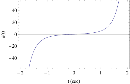
What interests us the most in this section, is to investigate which LQC-corrected theory can generate the bounce (34), near the bouncing point . It is conceivable that what we need to examine is the limit of the differential equations (28) and (29) presented in the previous section. We shall be interested in finding the first two functions of the perturbative -expansion of the previous section, namely and , assuming absence of any matter fluids. The Gauss-Bonnet invariant for the scale factor (34) reads,
| (35) |
and in the limit , this is approximately equal to,
| (36) |
Therefore, Eq. (36) can be explicitly solved with respect to the cosmic time ,
| (37) |
Notice that the small limit is equivalent to the small limit, so we shall take this observation into account in the rest of this section. In view of the above approximations, the differential equation that yields the function , namely Eq. (28), at the vicinity of the bouncing point is equal to,
| (38) |
which can be solved analytically, with the solution being of the following form,
| (39) |
where we kept only the leading order terms in the limit . Having at hand, we can easily obtain the function , by solving the second differential equation given in Eq. (29). In order to find an analytic approximation of the solution , we need to find an approximate form of the term,
| (40) |
appearing in the differential equation, where for notational simplicity we denoted the term with . The resulting expression of is quite lengthy and can be found in the Appendix, so here we quote only the simplified expression for , where we will keep only the dominant terms in the limit . In this limit, the term reads,
| (41) |
where stands for,
| (42) | ||||
Consequently, the differential equation that yields the solution for , namely Eq. (29), becomes,
| (43) |
which can analytically be solved to yield,
| (44) |
In conclusion, the final form of the small limit of the , which generates the bounce (34) near the bouncing point, is approximately equal to,
| (45) | ||||
Recall that the variable is equal to , so practically the limit measures the differences of the resulting LQC-corrected , in the limit where the LQC effects are strong, and therefore the LQC effects are contained in the term which is linear to . Indeed, the bounce is expected to occur when , and at that point, , and also, since is quite large, the parameter is quite small, and in the expansion, the most dominant term of the perturbative expansion, is of the order .
7.1.2 Hyperbolic Cosine Bounce Model
Another exponential bouncing model is described by the following scale factor,
For this model the Hubble rate is equal to,
Whence it follows immediately that,
Consider the following initial conditions for the Cauchy problem of Eq. (25),
where , are constants, and also satisfies . Then, for the functions , the following boundary conditions hold true:
| (46) |
The general solution of the unperturbed differential equation (28) has the form:
| (47) |
where , are constants of integration. Note that this solution is defined for . It is not difficult to find the values of the constants and :
Note that in the limit :
One can consider the first-order correction of the perturbative -expansion, namely . By considering Eqs. (46) and (47), the Cauchy problem for the differential equation (29) becomes:
| (48) |
| (49) |
It is easy to show that the solutions of the homogeneous differential equation are:
Then the solution of the inhomogeneous equation (48) can be written as:
where , are constants of integration. We can explicitly calculate the integral by using a new variable,
Then, the first correction can be written as follows,
| (50) |
where the functions and are defined as follows:
and are the Bernoulli numbers. Note that
From the initial conditions (49), it is easy to find the coefficients and , but due to lengthy and complicated expressions, we do not present the final solution to the Cauchy problem.
Before closing this section, we need to note that the following limiting cases hold true,
This implies that for the case , the first order correction is defined only in a neighborhood of the point . However, the case should be considered a separate way. It can be obtained, for example, in the formulation of the boundary value problem of Eq. (25):
At the same time it is easy to show that,
Note also that in this case, the first order correction can take finite values on the whole interval, where the function is defined, which is the following interval,
where is a finite constant.
Similarly, one can build corrections any other order for the model , but the expressions can be more complicated so we confine ourselves to the first two orders.
7.2 Power-law Bouncing Model
As a final example, we shall study another bouncing cosmology which is described by the following scale factor,
| (51) |
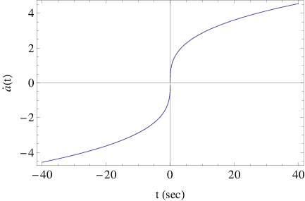
which is related to certain ekpyrotic models [17, 18]. The parameter is a real positive number which for the purposes of this section we choose it to satisfy , for reasons to be clear later on in this section. The cosmological evolution described by the scale factor (51) perfectly describes a bounce, meaning that before the bouncing point, we have , after the bouncing point and at the bounce , as can easily be checked by looking at Fig. 2, where we plotted the time dependence of the function , for 11 1 Notice that in principle if is not appropriately chosen, the scale factor might turn complex, so extra attention should be payed on this issue. and sec.
Since for general values of , it is quite difficult to analytically solve the differential equations (29), as in the symmetric bounce case, we shall investigate here which LQC-corrected gravity can describe the bounce (51) near the bouncing point , which can be arbitrarily chosen. Notice that when , the expression tends to zero, and this observation shall be useful in the following analysis. The Gauss-Bonnet invariant , for the scale factor (51) reads,
| (52) |
so as , the variable increases. Therefore the limit corresponds to the limit , and we shall use this correspondence in the analysis that follows. Solving Eq. (52), with respect to , we obtain,
| (53) |
and since , no inconsistency related to complex cosmological times occurs. The differential equation that yields the gravity is therefore equal to,
| (54) |
where we have set for simplicity and to be equal to,
| (55) |
The solution to the differential equation (54) is equal to,
| (56) |
Finally, we calculate the first order correction of the LQC-corrected gravity, namely the function , which easily follows if we use the analytic form of given in Eq. (56). However, since the exact solution is quite complicated and lengthy, we can approximate the resulting expression by recalling that the limit , corresponds to , so the larger term dominates in the expressions. For , the most dominant term is of the order , so is approximately equal to , and the resulting differential equation that yields the solution for , namely Eq. (29), becomes,
| (57) |
which can analytically be solved to yield,
| (58) |
8 Conclusions
In this paper, we extended the holonomy corrections formalism of LQC to Gauss-Bonnet modified gravity theories. Specifically, upon using the method of Lagrange multipliers, we constructed the classical dynamical cosmological equations in Gauss-Bonnet gravity, for a flat FLRW geometry. In addition, we extended LQC to Gauss-Bonnet gravity obtaining a holonomy corrected Friedmann equation, which contains all the dynamical information of the system. Then after explaining the reconstruction method in holonomy corrected Gauss-Bonnet gravity, we applied our formalism to certain cosmological scenarios, focusing in the realization of these cosmologies in the context of LQC-corrected gravity. The cosmological scenarios on which we emphasized are the bouncing cosmologies and the reason for that is that bouncing cosmologies provide a quite elegant alternative scenario to the inflationary paradigm. As we evinced, the resulting LQC-corrected dynamical equations are quite complicated, so we performed a perturbative expansion, using as a perturbation parameter, the parameter which is related to a very important physical quantity, the critical density , as . Practically, the parameter measures how quantum is the theory, and the smaller it is, the theory “stretches” in the more quantum era. In the perturbation series we used, we assumed that , so the leading order corrections we found, practically quantify the way that the LQC-corrected theory deviates from the classical theory. So iteratively, one can recover higher and higher corrections, being though less significant, depending on how fast tends to infinity.
Moreover, the possibility of having finite time singularities [39] and specifically mild types of singularities [40] is also quite interesting and should be extensively discussed.
Finally, the viability of the theories should also be checked and confronted with current observational data, but this task extends the purpose of this paper, which was the presentation of the method of LQC-corrected gravity, and its usefulness towards realizing cosmological scenarios. We hope however to discuss these topics in the near future.
Acknowledgments: This investigation has been supported in part by MINECO (Spain) projects MTM2011-27739-C04-01 (J.H.), FIS2010-15640 and FIS2013-44881 (S.D.O.) and Russian Ministry of Education and Science (S.D.O. and A.N.M.).
Appendix
References
- [1] R. Penrose, [Gen. Rel. Grav. 34, 1141 (2002)].
- [2]
A. Ashtekar and A. Barrau,
arXiv:1504.07559 [gr-qc];
B. Bolliet, J. Grain, C. Stahl, L. Linsefors and A. Barrau, Phys. Rev. D 91 (2015) 8, 084035 [arXiv:1502.02431 [gr-qc]];
L. C. Gomar, M. Martín-Benito and G. A. M. Marugán, JCAP 1506 (2015) 06, 045 [arXiv:1503.03907 [gr-qc]];
A. Barrau, M. Bojowald, G. Calcagni, J. Grain and M. Kagan, JCAP 1505 (2015) 05, 051 [arXiv:1404.1018 [gr-qc]].;
I. Agullo, A. Ashtekar and W. Nelson, Phys. Rev. Lett. 109 (2012) 251301 [arXiv:1209.1609 [gr-qc]].;
A. Ashtekar and P. Singh, Class. Quant. Grav. 28 (2011) 213001 [arXiv:1108.0893 [gr-qc]];
A. Ashtekar, Nuovo Cim. B 122 (2007) 135 [gr-qc/0702030];
M. Bojowald, Class. Quant. Grav. 26 (2009) 075020 [arXiv:0811.4129 [gr-qc]];
T. Cailleteau, A. Barrau, J. Grain and F. Vidotto, Phys. Rev. D 86 (2012) 087301 [arXiv:1206.6736 [gr-qc]];
A. Ashtekar, P. Singh, Class. Quant. Grav. 28, 213001 (2011) [arXiv:1108.0893 ];
A. Corichi, P. Singh, Phys.Rev. D80 (2009) 044024 [arXiv:0905.4949];
P. Singh, Class.Quant.Grav. 26 (2009) 125005 [arXiv:0901.2750];
A. Ashtekar, T. Pawlowski, P. Singh, Phys.Rev. D74 (2006) 084003 [gr-qc/0607039];
M. Bojowald, Class.Quant.Grav. 26 (2009) 075020 [arXiv:0811.4129] - [3] X. Zhang and Y. Ma, Phys. Rev. Lett. 106, 171301 (2011) [arXiv:1101.1752].
- [4]
X. Zhang and Y. Ma, Phys. Rev. D84, 064040 (2011)
[arXiv:1107.4921].
X. Zhang and Y. Ma, Front. Phys. 8, 80 (2013) [arXiv:1211.5024]. - [5] G. De Risi, R. Maartens and P. Singh, Phys. Rev. D76, 103531 (2007) [arXiv:0706.3586].
- [6] J. Amorós, J. de Haro and S.D. Odintsov Phys. Rev. D89, 104010 (2014) [arXiv:1402.3071].
- [7] J. de Haro, EPL 107, 29001 (2014) [arXiv:1403.4529].
- [8] K. Bamba, A.N. Makarenko, A.N. Myagki and S.D. Odintsov, Phys. Lett. B732, 349 (2014) [arXiv:1403.3242].
- [9]
M. Novello and S. E. P. Bergliaffa,
Phys. Rept. 463, 127 (2008)
[arXiv:0802.1634].
J. L. Lehners, Phys. Rept. 465, 223 (2008) [arXiv:0806.1245].
R. H. Brandenberger, Int. J. Mod. Phys. Conf. Ser. 01, 67 (2011) [arXiv:0902.4731].
R. H. Brandenberger, AIP Conf. Proc. 1268, 3 (2010) [arXiv:1003.1745].
D. Battefeld and P. Peter, [arXiv:1406.2790]. - [10]
M. Novello, S.E.Perez Bergliaffa, Phys.Rept. 463 (2008) 127 [arXiv:0802.1634];
C. Li, R. H. Brandenberger and Y. K. E. Cheung, Phys. Rev. D 90 (2014) 12, 123535 [arXiv:1403.5625 [gr-qc]].;
Yi-Fu Cai, E. McDonough, F. Duplessis, R. H. Brandenberger, JCAP 1310 (2013) 024 [arXiv:1305.5259];
Yi-Fu Cai, E. Wilson-Ewing, JCAP 1403 (2014) 026 [arXiv:1402.3009 ];
J. Haro, J. Amoros, JCAP 08(2014)025 [arXiv:1403.6396 ];
T. Qiu and K. C. Yang, JCAP 1011, 012 (2010) [arXiv:1007.2571 [astro-ph.CO]].;
T. Qiu, Class. Quant. Grav. 27, 215013 (2010) [arXiv:1007.2929 [hep-ph]]. - [11] Jean-Luc Lehners, Class.Quant.Grav. 28 (2011) 204004 [arXiv:1106.0172]
- [12]
N. Arkani-Hamed, Hsin-Chia Cheng, M. A. Luty, S. Mukohyama, JHEP 0405 (2004) 074 [hep-th/0312099]; A. Nicolis, R. Rattazzi, E. Trincherini,
Phys.Rev. D 79 (2009) 064036 [arXiv:0811.2197];
C. Deffayet , G. Esposito-Farese (Paris, Inst. Astrophys.), A. Vikman, Phys.Rev. D 79 (2009) 084003 [arXiv:0901.1314];
J. Khoury, B. A. Ovrut, J. Stokes, JHEP 1208 (2012) 015 [arXiv:1203.4562] - [13] M. Koehn, Jean-Luc Lehners, B. A. Ovrut, Phys.Rev. D 90 (2014) 025005 [arXiv:1310.7577]
- [14]
Yi-Fu Cai, D. A. Easson, R. Brandenberger, JCAP 1208 (2012) 020 [arXiv:1206.2382];
S. D. Odintsov and V. K. Oikonomou, Phys. Rev. D 91 (2015) 6, 064036 [arXiv:1502.06125 [gr-qc]] ’ - [15] Y. F. Cai, T. Qiu, Y. S. Piao, M. Li and X. Zhang, JHEP 0710 (2007) 071 [arXiv:0704.1090 [gr-qc]].
- [16]
R. H. Brandenberger, arXiv:1206.4196;
J. Quintin, Y. F. Cai and R. H. Brandenberger, Phys. Rev. D 90 (2014) 6, 063507 [arXiv:1406.6049 [gr-qc]];
Y. F. Cai, R. Brandenberger and X. Zhang, Phys. Lett. B 703 (2011) 25 [arXiv:1105.4286 [hep-th]];
Y. F. Cai, R. Brandenberger and X. Zhang, JCAP 1103 (2011) 003 [arXiv:1101.0822 [hep-th]];
K. Bamba, J. de Haro and S. D. Odintsov, JCAP 1302 (2013) 008 [arXiv:1211.2968 [gr-qc]];
J. de Haro, JCAP 1211 (2012) 037 [arXiv:1207.3621 [gr-qc]].;
S. D. Odintsov and V. K. Oikonomou, Phys. Rev. D 90 (2014) 12, 124083 [arXiv:1410.8183 [gr-qc]];
J. Haro, Europhys. Lett. 107 (2014) 29001 [arXiv:1403.4529];
Jaume de Haro, Yi-Fu Cai, arXiv:1502.03230;
K. Bamba, S. Nojiri, S. D. Odintsov, JCAP 0810 (2008) 045 [arXiv:0807.2575];
K. Bamba, A. N. Makarenko, A. N. Myagky, S. Nojiri and S. D. Odintsov, JCAP 1401 (2014) 008 [arXiv:1309.3748 [hep-th]]. ;
C. Barragan, G. J. Olmo and H. Sanchis-Alepuz, Phys. Rev. D 80 (2009) 024016 [arXiv:0907.0318 [gr-qc]]. - [17] S. D. Odintsov, V. K. Oikonomou and E. N. Saridakis, arXiv:1501.06591 [gr-qc].
- [18] V. K. Oikonomou, arXiv:1412.4343 [gr-qc]
- [19] S. D. Odintsov and V. K. Oikonomou, Phys. Rev. D 90 (2014) 12, 124083 [arXiv:1410.8183 [gr-qc]].
- [20]
J. Khoury, B. A. Ovrut , N. Seiberg, P. J. Steinhardt, N. Turok, Phys.Rev. D 65 (2002) 086007 [hep-th/0108187];
J. K. Erickson, D. H. Wesley, P. J. Steinhardt, N. Turok, Phys.Rev. D 69 (2004) 063514 [hep-th/0312009];
Yi-Fu Cai, Shih-Hung Chen, J. B. Dent, S. Dutta, E. N. Saridakis, Class. Quantum Grav. 28 (2011) 215011 [arXiv:1104.4349] - [21] J. Khoury, B. A. Ovrut, P. J. Steinhardt, N. Turok, Phys.Rev. D 66 (2002) 046005 [hep-th/0109050]
- [22] E. Wilson-Ewing, JCAP 1303 (2013) 026 [arXiv:1211.6269]
- [23]
D. Wands,
Phys. Rev. D 60, 023507 (1999)
[arXiv:9809062].
F. Finelli and R. Brandenberger, Phys. Rev. D65, 103522 (2002) [arXiv:0112249].
R. H. Brandenberger and R. Kahn, Phys. Rev. D 29 (1984) 2172.
R. H. Brandenberger, R. Kahn and W. H. Press, Phys. Rev. D 28 (1983) 1809.
V. F. Mukhanov, H. A. Feldman and R. H. Brandenberger, Phys. Rept. 215 (1992) 203.
J. Haro and J. Amoros, JCAP 1412, no. 12, 031 (2014) [arXiv:1406.0369 ].
Y. F. Cai, D. A. Easson and R. Brandenberger, JCAP 1208, 020 (2012) [arXiv:1206.2382].
J. Haro, JCAP 1311, 068 (2013) [Erratum-ibid. 1405, E01 (2014)] [arXiv:1309.0352].
E. Wilson-Ewing, JCAP 1303, 026 (2013) [arXiv:1211.6269].
Y. F. Cai and E. Wilson-Ewing, JCAP 1403, 026 (2014) [arXiv:1402.3009].
Y. F. Cai, Sci. China Phys. Mech. Astron. 57, 1414 (2014) [arXiv:1405.1369].
J. de Haro and J. Amoros, JCAP 1408, 025 (2014) [arXiv:1403.6396].;
R. H. Brandenberger, V. F. Mukhanov and A. Sornborger, Phys. Rev. D 48 (1993) 1629 [gr-qc/9303001].;
V. F. Mukhanov and R. H. Brandenberger, Phys. Rev. Lett. 68 (1992) 1969.;
L. Sebastiani and R. Myrzakulov, arXiv:1506.05330 [gr-qc].;
S. Myrzakul, R. Myrzakulov and L. Sebastiani, arXiv:1509.07021 [gr-qc]. - [24] E. Elizalde, J. Haro and S. D. Odintsov, Phys. Rev. D91, 063522 (2015) [arXiv:1411.3475].
- [25]
P. A. R. Ade et al. [Planck Collaboration],
Astron. Astrophys. 571, A16 (2014)
[arXiv:1303.5076].
P. A. R. Ade et al. [Planck Collaboration], Astron. Astrophys. 571, A22 (2014) [arXiv:1303.5082].
P. A. R. Ade et al. [Planck Collaboration], [arXiv:1502.01589].
P. A. R. Ade et al. [Planck Collaboration], [arXiv:1502.02114]. - [26] V. K. Oikonomou, arXiv:1509.05827 [gr-qc]
- [27] N. Deruelle, Y. Sendouda and A. Youssef, Phys. Rev. D80, 084032 (2009) [arXiv:0906.4983].
- [28] S. Nojiri and S.D. Odintsov, Phys. Lett. B631, 1 (2005) [arXiv:0508049].
- [29]
P. Singh, Class. Quant. Grav. 26, 125005 (2009)
[arXiv:0901.2750].
A. Corichi and P. Singh, Phys. Rev. D 78, 024034 (2008) [arXiv:0805.0136]; - [30] J. de Haro, JCAP 11, 037 (2012) [arXiv:1207.3621].
- [31] A. Ashtekar and P. Singh, Class. Quant. Grav. 28, 213001 (2011) [arXiv:1108.0893].
- [32]
A. Ashtekar, T. Pawlowski and P. Singh , Phys. Rev. D74, 084003 (2006).
A. Ashtekar, T. Pawlowski and P. Singh, Phys. Rev. D73, 124038 (2006) [arXiv:0604013].
A. Ashtekar, M. Bojowald and J. Lewandowski, Adv. Theor. Math. 7, 233 (2003).
T. Thiemann, Phys. Lett. B 380, 257 (1996) [arXiv:9606088].
T. Thiemann, Class. Quant. Grav. 15, 839 (1998) [arXiv:9606089].
T. Thiemann, Cambridge, UK: Cambridge Univ. Press. (2007) [arXiv:0110034]. - [33] M. Bojowald, Class. Quant. Grav. 26, 075020 (2009) [arXiv:0811.4129].
- [34] J. Haro and E. Elizalde, EPL 89, 69001 (2010).
- [35] P. Dzierzak, P. Malkiewicz and W. Piechocki, Phys. Rev. D80, 104001 (2009).
- [36]
P. Singh, K. Vandersloot and G. V. Vereshchagin,
Phys. Rev. D74, 043510 (2006)
[arXiv:0606032].
P. Singh, Phys. Rev. D73, 063508 (2006) [arXiv:0603043].
C. Rovelli and E. Wilson-Ewing, Phys. Rev. D D90, 023538 (2014) [arXiv:1310.8654]. - [37]
M. Bojowald and G.M. Hossain,
Phys. Rev. D77 023508 (2008) [arXiv:0709.2365].
T. Cailleteau, J. Mielczarek, A. Barrau and J. Grain, Class. Quant. Grav. 29 095010 (2012) [arXiv:1111.3535].
T. Cailleteau, A. Barrau, J. Grain and F. Vidotto, Phys. Rev. D86 087301 (2012) [arXiv:1206.6736].
T. Cailleteau, L. Linsefors and A. Barrau, Class.Quant.Grav. 31 125011 (2014) [arXiv:1307.5238]. - [38]
Nojiri S., Odintsov S.D., Phys. Lett. B631, 1 (2005) [arxiv:0508049].
Nojiri S., Odintsov S.D., Sasaki M., Gauss-Bonnet dark energy. Phys. Rev. D71, 123509 (2005) [arXiv:0504052].
Ratbay Myrzakulov, Diego Saez-Gomez, Anca Tureanu, Gen.Rel.Grav. 43, 1671-1684 (2011).
E. Elizalde, R. Myrzakulov, V. V. Obukhov and D. Saez-Gomez, Class. Quant. Grav. 27, 095007 (2010) [arXiv:1001.3636].
A.N. Makarenko, V.V. Obukhov, I.V. Kirnos, Astrophys.Space Sci. 343, 481-488 (2013) [arXiv:1201.4742]. - [39] S. Nojiri, S. D. Odintsov and S. Tsujikawa, Phys. Rev. D 71 (2005) 063004 [hep-th/0501025].
- [40]
J. D. Barrow and A. A. H. Graham,
Phys. Rev. D 91, no. 8, 083513 (2015)
[arXiv:1501.04090 [gr-qc]].
S. Nojiri, S. D. Odintsov and V. K. Oikonomou, Phys. Rev. D 91 084059 (2015) [arXiv:1502.07005 [gr-qc]].
S. Nojiri, S. D. Odintsov, V. K. Oikonomou and E. N. Saridakis, arXiv:1503.08443 [gr-qc].