Gaussian Process Regression with Location Errors
Abstract
In this paper, we investigate Gaussian process regression models where inputs are subject to measurement error. In spatial statistics, input measurement errors occur when the geographical locations of observed data are not known exactly. Such sources of error are not special cases of “nugget” or microscale variation, and require alternative methods for both interpolation and parameter estimation. Gaussian process models do not straightforwardly extend to incorporate input measurement error, and simply ignoring noise in the input space can lead to poor performance for both prediction and parameter inference. We review and extend existing theory on prediction and estimation in the presence of location errors, and show that ignoring location errors may lead to Kriging that is not “self-efficient”. We also introduce a Markov Chain Monte Carlo (MCMC) approach using the Hybrid Monte Carlo algorithm that obtains optimal (minimum MSE) predictions, and discuss situations that lead to multimodality of the target distribution and/or poor chain mixing. Through simulation study and analysis of global air temperature data, we show that appropriate methods for incorporating location measurement error are essential to valid inference in this regime.
keywords
Gaussian processes , measurement error , Kriging , MCMC , geostatisticsand
Harvard University??
1 Introduction
Gaussian process models assume an output variable of interest varies smoothly over an input space (e.g., percipitation totals across geographical coordinates, crop yield across factor levels of an experimental design). Such models appear frequently in areas as diverse as climate science [Mardia and Goodall (1993)], epidemiology [Lawson (1994)], and black-box problems such as computer experiments, and Bayesian optimization [Sacks et al. (1989); Srinivas et al. (2009)]. See Stein (1999); Cressie and Cassie (1993); Banerjee, Carlin and Gelfand (2014) and Gelman et al. (2014) for more detailed treatments.
Noisy spatial input data are common in many applications; for example, geostatistical data is often imprecisely spatially referenced, “binned” to the nearest latitude/longitude grid point, or referenced to maps with distorted coordinates [Veregin (1999); Barber, Gelfand and Silander (2006)]. Accounting for measurement error on covariates in the context of regression models is a well studied theme [Carroll et al. (2006)]; however, despite their importance in applications, surprisingly little work has been done on interpolation or Gaussian process regression problems in the presence of (spatial) location measurement error. As we show in this paper, Gaussian process models do not straightforwardly extend to incorporate input measurement error, and simply ignoring noise in the input space can lead to poor performance.
Previous research on such error sources has mostly focused on demonstrating their existence and quantifying their magnitude [Bonner et al. (2003); Ward et al. (2005)]. For regression problems, Gabrosek and Cressie (2002) (and later Cressie and Kornak (2003)) adjust Kriging equations for the presence of location errors, and Fanshawe and Diggle (2011) further develop research for this regime to include problems where the locations of future observations or predictions are subject to error. Location errors have also been studied in the context of point process data [Zimmerman and Sun (2006); Zimmerman, Li and Fang (2010)].
Properly accounting for location errors is essential for optimal interpolation and uncertainty quantification, as well precise and efficient parameter estimation when parameters of the covariance function are unknown. Using theoretical results and extensive simulations, our paper provides guidelines on situations when location errors are most impactful for data analysis, and suggestions for incorporating this source of error into inference and prediction. We expand the research in Cressie and Kornak (2003) on best linear unbiased prediction (Kriging) to include procedures for obtaining interval forecasts and for quantifying the cost of ignoring location errors. We also discuss Markov Chain Monte Carlo (MCMC) methods for optimal (minimum mean squared error (MSE)) predictions, which average over the conditional distribution of (latent) location errors given the observed data.
Section 2 establishes notation and describes the basic model with location errors used throughout the paper. In Section 3, we discuss Kriging using the covariance structure of the location-error induced process. Section 4 considers MCMC methods for obtaining minimum MSE predictions, and thus improving upon Kriging. We compare these methods through simulation study in Section 5, and explore an application to interpolating northern hemisphere temperature anomolies in Section 6. The proofs of all of the theoretical results are given in an Appendix.
2 The Model
We will write to denote a -vector of locations in the input space , and as the associated vector of observations at . Similarly, we will denote , or simply where are unobserved locations. The process is called a Gaussian process if, for any , is jointly Normally distributed. Typically, the form of this joint distribution is specified by a deterministic or parametric mean function (for now, taken without loss of generality to be 0) and a covariance function , so that
| (1) |
For to be a valid covariance function, the covariance matrix in Equation (1) must be positive semi-definite for all input vectors .
Gaussian process regression is primarily used as a method for interpolating (predicting) values at unobserved points in the input space, given all available observations. Such conditional distributions are easily obtained by exploiting the joint normality of the response at observed and unobserved locations:
| (2) |
In Equation (2), denotes the covariance matrix of , denotes the covariance matrix between and .
When the locations in the input space are affected by error, we observe a surrogate process ,
where is a known location in and is unobserved location error. The problem of Gaussian process regression with location errors addressed in this paper is to predict at unobserved (exact) locations given observations from the noise-corrupted process .
When is assumed to be a Gaussian process, there is no nontrivial structure for that results in being a Gaussian process. Additionally, it is not possible to write as a convolution of and a white noise process as differences between the surfaces and will generally be correlated across space, i.e., . Gaussian process regression with location errors therefore cannot be thought of as a classical or Berkson errors-in-variables problem [Carroll et al. (2006)]. Interestingly, in some cases, the process may be more informative for prediction at a new location than the process is. Thus, appropriate methods can deliver lower MSE interpolations in a location-error regime than the MSE of the usual methods in an error-free regime.
3 Kriging the Location Error Induced Process
As shown in Cressie and Kornak (2003), the second moment properties of can be used to perform Kriging (they named this “Kriging adjusting for location error” or KALE), noting that measurement errors induce a new covariance function
| (3) |
The expectation here is taken over the input errors , which are assumed to have some joint distribution . The following result shows that if is a valid covariance function, then so is , regardless of the error distribution .
Proposition 3.1.
Assume for all and , , where is any family of probability measures on . Then is a valid covariance function if is.
Regardless of the form of , always exhibits the “nugget” effect, or discontinuities in the covariance function [Matheron (1962)] In fact, several authors cite location/positional error as a justification for including a nugget term in an arbitrary covariance function [Cressie and Cassie (1993); Stein (1999)], alongside independent measurement error in observing the response, . Location errors, however, cause to differ from throughout the spatial domain (this is shown in Figure 1), meaning that while they induce a nugget, a nugget term alone cannot capture the effect of location errors.
Using , we get the Kriging estimator adjusting for location error for at an unobserved location of :
| (4) |
In Equation (4), and respectively denote the covariance matrices corresponding to the kernels and . The quantity is the best linear unbiased predictor for (in terms of MSE) and has all the usual Kriging properties. When there are no location errors, the Kriging estimator is equivalent to the conditional expectation of given (see Equation (2)).
In general, the covariance functions and can be evaluated using Monte Carlo integration by repeatedly sampling from . For several common combinations of covariance function and location error models, however, it is possible to arrive at the expressions in Equation (3) in closed form. In particular, if
then we can define a random variable and find its moment generating function . If we can evaluate at , then this yields . For instance, for the squared exponential covariance function and Normal location errors , has a scaled noncentral distribution and
| (5) |
with a similar expression for . Thus the covariance function for is also squared exponential (it is not generally true that and will share the same functional form). Note, however, that not all parameters are identifiable—we must know at least one of in order to estimate the others.
Interestingly, it is possible for the KALE to yield lower MSE predictions than those given from an error-free regime, where and . In other words, can be more informative than for predicting . Heuristically, this happens when is more strongly correlated with than is . Below we characterize the conditions for observing this phenomenon in a simple model with one observed data point (Figure 1 provides an illustration); it seems difficult to generalize this to larger observed location samples and covariance/error structures.
Proposition 3.2.
Assume , , for all , and . Without location error (), the MSE in predicting from is . There exists such that if and only if .
3.1 Interval predictions
For many applications of Gaussian process regression, particularly in geostastics and environmental modeling, both point and interval predictions are of interest. However, Kriging, being strictly a moment-based procedure, does not provide uncertainty quantification for predictions other than variance. In a location-error Gaussian process regime, KALE predictions will always be non-Gaussian, thus variance alone is not sufficient to provide distributional or interval predictions.
However, it is relatively straightforward to derive confidence intervals for predictions at unobserved locations given measurements at locations . The following proposition provides the exact distribution function (CDF) for prediction errors , which can be inverted to obtain a confidence interval for based on .
Proposition 3.3.
Let
Then
| (6) |
where is the CDF of the standard Normal distribution.
It may be necessary to evaluate Equation (6) using Monte Carlo; if so, it is practical to use the same draws of when evaluating different quantiles , as this guarantees a Monte Carlo estimate of the distribution function be non-decreasing.
While intervals based on (6) provide exact coverage (modulo Monte Carlo error), such coverage is achieved by averaging over all data, both observed () and unobserved () as well as the location errors, . This is in contrast to usual interval estimates from Gaussian process regression without location error, which are exact probability statements conditional on the observed data . The reason this is an important distinction is because the usual Gaussian process conditional probability intervals yield the proper coverage rate across multiple prediction intervals (when predicting at a collection of unobserved locations ), whereas the confidence intervals corresponding to KALE may not.
3.2 Advantages over Kriging while Ignoring Location Errors
Failing to adjust for location errors when Kriging (Cressie and Kornak (2003) called this “Kriging ignoring location errors” or KILE) can lead to poor performance. A data analyst ignoring the location errors will use (see Equation (2))
| (7) |
Since is the best linear unbiased estimator for and is also an unbiased linear estimator, KALE dominates KILE and always yields a reduced MSE. Figure 2 illustrates the disparity in MSE for a simple model; intuitively, the relative cost of ignoring location errors increases as the magnitude of the location errors increases. We also see in panel (B), illustrating Proposition 3.2, that for small values of , the MSE for both KALE and KILE decreases in .
Besides yielding suboptimal predictions relative to KALE, ignoring location errors also leads to an estimator for that is not self-efficient [p. 549, Meng (1994)]. Following Meng (1994), an estimator for parameter is self-efficient if for any and subset of the observed data , we have
Thus, roughly speaking, self-efficient estimators are those that cannot be improved by using only a subset of the original data [Meng and Xie (2014)].
The following theorem states that the KILE MSE is unbounded as a function of any single spatial location for . This is a stronger result than just the lack of self-efficiency. A consequence of Theorem 3.4 is that, assuming only simple continuity conditions on the covariance function and location error model, the KILE MSE can always increase when observing more data, regardless of the locations of the existing observations or the locations at which we want to make predictions.
Theorem 3.4.
Suppose that the following conditions hold:
- •
is continuous and bounded in ,
- •
the location error model satisfies for all and sequences such that ,
- •
and for all .
Let be the KILE estimator for given . Then for any , , and , there exists such that .
Note that the condition that is continuous excludes a nugget term from the distribution of . We prove Theorem 3.4 (in the Appendix) by showing that when observed locations are very close together, the corresponding covariance matrix is nearly singular, and this increases MSE. Without location errors, the usual Kriging estimator does not exhibit this behavior since the difference between values of for points that are close together also converges in probability to 0. This is not the case for the noise-corrupted process, as does not converge to 0.
Simulation results suggest that even when contains a nugget term , KILE is still not self-efficient, and additional observations can increase MSE. Figure 3 illustrates the change in MSE as a function of the location of an additional observation of . Following Theorem 3.4, we see the MSE is unbounded when . But even when , it is possible for an additional observation to (slightly) increase MSE.
3.3 Parameter Estimation for Kriging
In typical applied settings, some or all parameters of the covariance function are unknown and must be estimated by the analyst in order to obtain Kriging equations. For Gaussian process models without a location error component, parameter estimation can be accomplished using likelihood methods. This can be computationally challenging for large data sets, as each likelihood evaluation requires a Cholesky factorization of the covariance matrix (or equivalent operations), which is except in special cases. An alternative is to choose parameters by maximizing goodness of fit between the empirical variogram and the theoretical (parametric) variogram, though this is less efficient for parametric Gaussian models.
Location errors present challenges for both such procedures as the covariance function for the observed provess (3) may not be available in closed form, meaning neither the likelihood function or variogram can be evaluated exactly. While Monte Carlo methods surely offer effective approaches in theory [Fanshawe and Diggle (2011)], they muliply the computational expense of the problem, as each evaluation of the likelihood requires matrix factorizations, where is the number of Monte Carlo samples used to approximate the likelihood. Cressie and Kornak (2003) advocate a pseudo-likelihood procedure [Carroll et al. (2006)] that uses a Gaussian likelihood approximation based on the first two moments of ,
| (8) |
where we write to explicitly mark the dependence of the covariance function on unknown parameters . This pseudo-likelihood requires inverting only once per pseudo-likelihood evaluation, even when is computed by Monte Carlo.
We can work out inferential properties of the maximum pseudo-likelihood estimator . First, it is straightforward to check that the pseudo-score pertains to an unbiased estimating equation:
| (9) |
Moreover, one can show the covariance matrix of the pseudo-score is given by
| (10) |
using the notational abbreviations , , and . Lastly, the expected negative Hessian of the log pseudo-likelihood is
| (11) |
If there are no location errors (), is an exact likelihood and the second term in the right hand side of Equation (10) vanishes so that , confirming the second Bartlett identity [Ferguson (1996)]. For non-zero location errors, however, we construct the Godambe information matrix as an analog to the Fisher information matrix [Varin, Reid and Firth (2011)],
Evaluating for different location error models illustrates the information loss in estimating covariance function parameters relative to the error-free case, where is equivalent to the Fisher information matrix.
General theory of unbiased estimation equations [Heyde (1997)] suggests the asymptotic behavior of the pseudo-likelihood procedure satisfies
| (12) |
However, Expression (12) does not hold in general even in an error-free regime , as asymptotic results for Gaussian process covariance parameters depend on the spatial sampling scheme used and the specific form of the covariance function [Stein (1999)]. We nevertheless expect (12) to hold for suitably well-behaved processes under increasing-domain asymptotics. Guyon (1982) gives an applicable result when locations are on a lattice. We are not aware of other theoretical results in this context.
4 Markov Chain Monte Carlo Methods
Markov Chain Monte Carlo methods offer an alternative to Kriging for prediction in a regime with noisy inputs. They allow us to compute the MSE-optimal prediction
| (13) |
which will dominate the KALE estimator (4) in terms of MSE for any model and set of observed and predicted locations. The optimality of in (13) is due to the fact that the conditional mean obtains the minimum MSE for any estimator of that is a function of . This estimator is not linear, and MCMC methods are necessary for evaluating (13) as the density for the conditional distribution will not be available in closed form (no possible “conjugate“ form for the distribution of is known to us). When model parameters, such as in the covariance function or the distribution of are unknown, the distribution implicitly averages over the posterior distributions of such parameters.
MCMC methods also allow us to compute prediction intervals such that . When the covariance function and location error model are known, these intervals are exact probability conditional probability statements, providing a stronger coverage guarantee than that achieved with the KALE procedure in Proposition 3.3, where coverage is achieved only by averaging over .
4.1 Distributional Assumptions
MCMC inference for (13) requires the assumption that is Gaussian. While this is a common assumption in practice and has been assumed throughout this paper, it is not necessary to derive the KALE equations and their MSE (but it is necessary to produce coverage intervals as in Proposition 3.3). Thus, Kriging approaches, including KALE, are attractive when there is information about the joint distribution of beyond its first two moments.
In this scenario, however, we can still advocate—from a decision-theoretic perspective—a Gaussian assumption when the goal of the analysis is minimum MSE prediction. Specifically, let be a choice of joint distribution for with the appropriate first two moments and . The minimum MSE prediction of assuming is the conditional mean . Let be the risk (MSE) of this minimum MSE predictor under the assumption that when in fact ; that is,
Thus represents the risk (MSE) in a misspecified joint distribution for , where the analyst assumes , but in fact . We then have the following proposition, based on Theorem 5.5 of Morris (1983):
Proposition 4.1.
Let be Gaussian. Then for all we have
Unlike traditional decision theory problems, here we are fixing the estimator (Kriging), and considering the costs of different distributional assumptions (). Given that the analyst has decided to use Kriging for predicting , then the risk in making an incorrect distributional assumption is . This reflects the fact that the Kriging MSE depends only on the first two moments of . However, there is an “opportunity cost” in making any non-Gaussian assumption for , which represents the reduction in MSE under that could be achieved by using a different estimator other than Kriging.
Obviously, if there is a strong reason to believe a non-Gaussian is true, then analysis should proceed with this assumption, ideally leveraging an estimator that is optimal under these assumptions (instead of Kriging). However, without strong distributional knowledge, the analyst can assume Gaussianity without risking increased MSE or paying an opportunity cost for using an inefficient method.
4.2 Hybrid Monte Carlo
Hybrid Monte Carlo [Neal (2005)] is well-suited for the problem of sampling in order to evaluate (13). This is because while is computationally expensive (requiring inversion of the covariance matrix ), the gradient is a relatively cheap byproduct of this calculation. Often the conditional distribution is correlated across components, making gradient-based MCMC methods more efficient for generating samples. Other gradient-based MCMC sampling methods, such as the Metropolis-adjusted Langevin algorithm [Roberts et al. (2001)] and variants, may also be well-suited to this problem.
Bayes rule provides , where here represents any unknown parameter(s) of the covariance function . In most situations it will be reasonable to assume and are independent a priori—this is trivially true in the case that is assumed known. Assuming this, and recognizing that is Gaussian, we can write the log posterior and its gradient:
The computational cost of both the likelihood and gradient are dominated by solving (e.g., Cholesky factorization), which is . Every likelihood evaluation computes this term, which can then be re-used in the gradient equations. Thus, the computational cost of computing both the likelihood and gradient remains .
4.3 Multimodality
The posterior distribution is often multimodal, more so if the distrubution is diffuse. This is because if there is a local mode at , there may be a local mode at any such that , as the likelihood is constant for such . In particular, for isotropic covariance models, the likelihood is constant for additive shifts in or rotations of , as these operations preserve pairwise distances. Additionally, multimodality can be induced by the many-to-one mapping of the set of true locations to the set of observed locations . For instance, with and an isotropic covariance function, for any choice of we get the same likelihood with and . Moreover, for fixed , for many common covariance functions it is possible for the posterior of to be multimodal [Warnes and Ripley (1987)].
HMC (and other gradient MCMC methods) can efficiently sample from multiple modes, however this becomes difficult when the modes are isolated by regions of extremely low likelihood [Neal (2011)]. Isolated modes can occur in the location-error GP regime. For example, assume one-dimensional locations () and an isotroptic covariance model with known parameters and nugget . Marginally, as , ; that is, the scaled difference must be reasonably small. When this is not the case (e.g. ), then the log-likelihood asymptotes at almost surely. Thus, the Markov chain can only sample such that the ordering of is preserved. Note that when , while the log-likelihood may still asymptote at , this no longer constrains the space of (except on sets with measure 0).
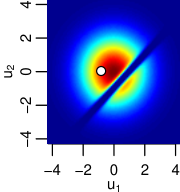
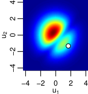
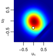
Figure 4 demonstrates the modal behavior for this simple example with and . When location errors are large in magnitude and the nugget tern is small, the modes of are separated by a contour of near 0 density (panel A). A higher nugget increases the density between the modes, making it easier for the same MCMC chain to travel between them (panel B). Decreasing the magnitude of the (Gaussian) location errors, , puts more mass on a single mode, as the unimodal distribution has a greater influence on (panel C).
Thus, as with any MCMC application, for the location-error GP problem it is advisible to run separate chains in parallel, with different, diffuse starting points, and monitor mixing diagnostics [Gelman and Shirley (2011)]. Multiple chains failing to mix is likely a symptom of multiple isolated modes, in which case we should modify the HMC algorithm to include tempering [Salazar and Toral (1997)] or non-local proposals that allow for mode switching [Qin and Liu (2001); Lan, Streets and Shahbaba (2013)]. Another strategy to overcome multiple isolated modes is importance sampling: as Figure 4 shows, increasing the nugget variance increases the density between modes. If we generate samples according to where is the density corresponding to for some fixed , then it is straightforward to compute importance weights . This is because is easy to compute from (and vice versa) using the Woodbury formula. Either standard importance sampling, or Hamiltonian importance sampling [Neal (2005)], could be used to generate parameter estimates, point/interval predictions, and any other posterior estimates of interest.
5 Simulation study
We compare Kriging (both KALE and KILE) and HMC methods for point/interval forecasts for Gaussian process regression in a simulation study. For various combinations of parameter values for the covariance function and location error model we simulate observations where and make predictions for values of at unobserved locations: .
We simulate data using the squared exponential covariance function and an i.i.d. Gaussian location error model . The squared exponential covariance function and Gaussian location error model combine to form a convenient regime, as we can evaluate in closed form (5). Without loss of generality, we can use for all simulations as it is simply a scale parameter. We consider a dimensional location space, . On a grid, we randomly select 54 locations at which we observe , and target the remaining 10 locations for interpolating . Figure 5 illustrates a range of data samples for processes used in our simulations on this space, while Table 1 provides a full summary of all the parameter value combinations we consider. Data from each parameter combination is simulated 100 times.
| Parameter | Values simulated | Prior support |
|---|---|---|
| 1 | ||
| 0.001, 0.01, 0.1, 0.5, 1, 2 | ||
| 0.0001, 0.01, 0.1, 0.5, 1 | ||
| 0.0001, 0.01, 0.1, 0.5, 1 |
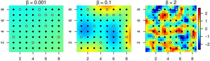
We evaluate the three prediction methods—KALE, KILE, and HMC—using both adjusted root mean squared error (RMSE) and the coverage probability of a interval. “Adjusted” RMSE is based on the MSE with subtracted out, as this term appears in the MSE for any prediction method. For every parameter combination of interest used, these statistics are calculated first by averaging over each of the prediction targets in each simulated draw of new data, and then over the independent data draws.
Both evaluation statistics can be evaluated more precisely during simulation by utilizing a simple Rao-Blackwellization. For iteration , instead of drawing in addition to and calculating , we simply condition on the simulated location errors to get . Similarly, to calculate coverage of an interval for , for iteration we use
HMC is implemented using the software RStan [Stan Development Team (2014)], which implements the “no-U-turn” HMC sampler [Homan and Gelman (2014)]. 10000 samples were drawn during each simulation iteration, which (for most parameter values) takes a few minutes on a single 2.50Ghz processor.
5.1 Known covariance parameters
We first simulate point and interval prediction for KALE, KILE, and HMC using the same parameter values that generated the data. By doing so, we leave aside the issue of parameter inference and simply compare the extent to which different methods leverage the information in the location-error corrupted data to infer . Figure 6 compares RMSE for the three methods when there is a very small nugget, .
We can see that there is little difference among the three methods when is sufficiently small (), or when is sufficiently large (). This makes sense, as in the former case, with small location errors the potential improvement over KILE (which is exact for ) is negligible, and in the latter case, observations are too weakly correlated for nearby points to be informative. Larger values of give KALE a significant reduction in RMSE versus KILE, with the reduction as large as for the case of large magnitude location errors () and a moderately smooth signal ().
The idea of a moderately smooth signal requires further elaboration: for a given , when is very smooth ( very small), the process is roughly constant within small neighborhoods, meaning and location errors are less of a concern for accurate inference and prediction. On the other hand, when is very large and the process is highly variable in small regions of the input space, location errors are less of a concern because there is very little information in the data to begin with. Location errors are most influential when the process has more moderate variation across neighborhoods corresponding to the plausible range of the location errors.
HMC offers further reductions in RMSE over KALE in roughly the same regions of the parameter space in which KALE improves over KILE, although the additional improvement is less dramatic. The maximum RMSE reduction we observe is about , once again for a moderately smooth signal with larger magnitude location errors.
When the nugget variance is increased (Figure 7 shows results for ), differences in RMSE among the three methods become smaller (the differences are wiped out entirely at , which is not pictured). This is not due to a shared term in the RMSE value for all methods, as this is subtracted out. Rather, the similarity of all three methods reflects the fact that a larger nugget leaves less information in the data that can be effectively used for prediction. However, the differences that we do observe (both comparing KALE to KILE and HMC to KALE) occur primarily when the magnitude of location errors is large.
In the case where all parameters are fixed and known, both KALE and HMC produce intervals with exact coverage (subject to Monte Carlo or numerical approximation errors) in all simulations. KILE, however, can severely undercover in the presence of location errors. Figure 8 shows coverage as low as when the magnitude of the location errors is high (), , and the nugget variation is minimal (). Undercoverage still persists in this region of the parameter space for , the largest nugget variance used in our simulations.
5.2 Unknown covariance parameters
In typical applied settings, the analyst will not know model parameters such as those of the covariance function (), the nugget variance , or even the variance of the location errors . Due to identifiability issues with our choice of covariance function in this simulation (5), we assume is known but estimate all other parameters before making predictions at unobserved locations.
For KILE and KALE, parameter estimation is accomplished through maximum (pseudo-) likelihood, as in (8). Parameter estimates are then plugged into Kriging equations (4)–(7) to obtain corresponding point and interval estimates. Because and are both squared exponential (5), the pseudolikelihood estimation procedure estimates the same covariance function for , however the estimated parameters (and therefore Kriging equations, based on ) will differ. The plug-in approach ignores uncertainty in parameter estimates, so plug-in MSE estimates will be too optimistic. Various techniques exist for adjusting MSE from estimated parameters [Smith (2004); Zhu and Stein (2006)], though there is no need to incorporate such techniques into our analysis since exact (up to Monte Carlo error) MSEs are provided by simulation.
For HMC, we supply unknown parameters with prior distributions and sample parameters and predictions jointly from the posterior distribution . The priors we use are flat over a reasonable range (see Table 1), which guarantees both a proper posterior and a posterior mode that agrees with the maximum likelihood estimate of . This second condition supports fair comparisons between predictions derived from HMC parameter estimates versus those based on the maximum (psueolikelihood) parameter values.
Figure 9 provides the relative RMSE of KALE vs. KILE, and HMC vs. KALE, for predictions when parameters must first be estimated (using ). We notice that there does not appear to be a great advantage in KALE over KILE when parameters are first estimated. This is because, as mentioned earlier, the marginal process still has a squared exponential covariance function 5, so Kriging equations for KALE and KILE will be very similar. On the other hand, we notice a modest improvement when using HMC over Kriging, except in a small region of the parameter space ( and ).
When the nugget variance is increased to , we see the results in Figure 10. We still see relatively similar performances from KALE and KILE. HMC offers a small improvement over KALE when , though for we actually see significantly higher MSEs with HMC. At the process is extremely smooth, as the most distant pairs of observations still have a correlation of . We are thus more concerned with overestimating than underestimating it; as the former shrinks predictions towards 0 while the latter shrinks towards (approximately) the mean of all observations. As we use a flat prior for , where almost all mass is located , the posterior tends to overestimate , leading to draws with relatively high MSE.
Neither Kriging or HMC guarantees prediction intervals with the correct coverage in the regime where parameters must first be estimated (though HMC would give proper “Bayes coverage” when simulating according to the prior used). We nevertheless present coverage results in Figures 11–13. While we do not expect any method used to provide exact coverage, Kriging (both KALE and KILE) suffer from significant undercoverage for some regions of the parameter space, while HMC is consistent in offering at least coverage throughout our simulations. In a regime without location errors, Zimmerman and Cressie (1992) advocate Bayesian procedures under non-informative priors over frequentist procedures in order to obtain interval estimates with good coverage; our simulation results, albeit in the context of location errors, agree with this finding.
5.3 Summary
Our simulation results confirm the theoretical guarantee of KALE dominating KILE in prediction MSE when the covariance function is known, and furthermore HMC dominating KALE. The magnitude of differences in MSE between these methods is greatest when the process is moderately smooth relative to the spatial sampling (e.g., ), when the magnitude of location errors is largest, and when nugget variation is smallest. For such regions of the parameter space, KILE fails to deliver prediction intervals with proper coverage, whereas KALE and HMC can give valid prediction intervals for any parameter values.
An important consequence in adjusting for location errors with a known covariance function is the corresponding adjustment to the nugget. The discussion in (Sections 3.6 and 3.7 of) Stein (1999) emphasizes the importance of correctly specifying the high-frequency behavior of the process when interpolating (correctly specifying the low-frequency behavior is less crucial), including the nugget term. Estimating parameters, including the nugget term , implicitly corrects for model misspecification when ignoring location errors. Thus we see little difference in predictive performance between KALE and KILE when parameters are first estimated. Depending on the choice of prior, KALE/KILE may give lower MSE predictions than HMC, which averages over posterior parameter uncertainty; however, interval coverage is better for HMC (using weak prior information) than for KALE/KILE.
6 Interpolating Northern Hemisphere Temperature Anomolies
To illustrate the methods discussed in this paper, we consider interpolating northern hemisphere temperature anomolies during the summer of 2011 using the publicly available CRUTEM3v data set11 1 http://www.cru.uea.ac.uk/cru/data/temperature/ [Brohan et al. (2006)]. Figure 14 shows our data. These data are used in geostatistical reconstructions of the Earth’s temperature field, which interpolate temperatures at unobserved points in space-time in order to better understand the historical behavior of climate change (see, e.g., Tingley and Huybers (2010) and Richard et al. (2012)). Each observation is a spatiotemporal average: temperature readings are averaged over the April–September period and each longitude-latitude grid cell. These values are then expressed as anomolies relative to the global average during the period 1850–2009, which is calculated using an ANOVA model [Tingley (2012)]. Apart from this spatiotemporal averaging, numerous other preprocessing steps adjust this data for differences in altitude, timing, equipment, and measurement practices between sites, along with other potential sources of error; please see Morice et al. (2012) and Jones et al. (2012) for more details.
Our analysis, restricted to interpolating a single year of data, and without using external data such as temperature proxies [Mann et al. (2008)], is intended as a proof of concept rather than as a refinement or improvement to existing analyses of these data. We wish to illustrate the potential impact of location errors on conclusions drawn from these data.
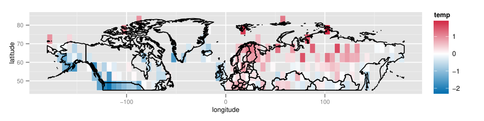
The “gridding”, or spatial averaging across cells, complicates analyses using Gaussian process models [Director and Bornn (2015)]. However, assuming a smooth temperature field, we know that the recorded spatial average must be realized exactly at some location in each grid box (closer to the center if a lot of points have been averaged together). This frames the spatial averaging problem as a location measurement error problem: instead of observing the temperature at each grid center , we observe the temperature at an unknown location displaced from the grid center: .
Following Tingley and Huybers (2010), we assume an exponential covariance function for , where distance is calculated along the Earth’s surface. As is given in terms of longitude/latitude (), this has the form
| (14) |
where is the radius of the earth (in km). At higher latitudes (), the centers of each grid cell are closer together, so nearby observations are more strongly correlated. The nugget term represents some combination of measurement error in temperature readings and high-frequency spatial variation that is inestimable using the gridded observation samples.
We assume the following model for location errors , which are additive displacements of longitude/latitude coordinates :
| (15) |
This prior is equivalent to assuming that distance along the Earth’s surface (great-circle distance) between each grid center and the corresponding observation location has a scaled chi distribution, . Combining (15) and (14), we use Monte Carlo to compute .
We treat parameters as unknown, but fix . At this value, the median magnitude of the location errors in great-circle distance is 102km, which is consistent with analyzing the coordinates of the temperature recording sites used to compile the CRUTEM3v data22 2 Station locations are vieweable at https://www.ncdc.noaa.gov/oa/climate/ghcn-daily/.
6.1 Kriging
We first apply Kriging approaches to interpolate the CRUTEM3v data, both adjusting for and ignoring location errors (15). Because parameters are unknown, we first need to estimate them using maximum likelihood (when ignoring location errors) or maximum pseudo-likelihood (8) (when adjusting for location errors). These can then be plugged in to covariance functions and to obtain “empirical” Kriging equations we can use for interpolation [Zimmerman and Cressie (1992)].
We find small differences in parameter estimates when ignoring location errors (assuming ) and adjusting for them (assuming ):
| 0 | 1.1671 | 0.0747 | |
| 7500 | 1.1649 | 0.0699 |
Consequently, when we interpolate data at the centers of grid cells for which no data was observed, we see differences between the KALE and KILE approaches. Figure 15 shows the differences between KALE and KILE interpolations (both point and interval estimates). Relative to the range of the data (most anomolies are in the interval ), the discrepency between KALE and KILE does not seem very significant.
6.2 HMC
Using HMC, parameter inference and interpolations are made simultaneously. The resulting point and interval predictions differ substantially from the Kriging results. However, because HMC incorporates parameter uncertainty in predictions, this comparison is not sufficient to illustrate the impact of location errors on conclusions from this data. A more appropriate comparison is between HMC with a location error model (), and HMC assuming with no location errors (). These results are plotted in Figure 16.
Using HMC, accounting for location errors produces more significant differences in inference/prediction than was observed for Kriging. This is particularly true for interval predictions, where adjusting for location errors yields intervals as much as 0.1 wider, which is a significant discrepency when most observations lie in .
Figure 17 shows posterior densities for unknown parameters of the covariance function based on HMC draws from the and models (the Kriging estimates of these parameters are vertical lines). HMC under location error model () gives slightly larger estimates than when using , meaning observations are inferred to be less strongly correlated. This yields prediction intervals that tend to be wider (see Figure 16). The most extreme descrepencies occur in the arctic, where distances between grid points are closest. The fact that modeling location errors adds additional uncertainty to arctic predictions is of particular interest to climate scientists, as accurate climate reconstruction for the arctic region is essential for understanding recent climate change patterns [Cowtan and Way (2014)].
The difference between predictions obtained under the and models using HMC suggests that modeling location errors, even when they are small in magnitude, meaningfully impacts parameter estimates and predictions at unobserved locations. The fact that results for HMC (assuming ) also differ from the results using KALE, while the KILE results do so less, demonstrates that moment procedures such as Kriging may be ineffective in adjusting for these errors.
7 Conclusion
In this paper, we have explored the issue of Gaussian process regression when locations in the input space are subject to error. Even when location errors are quite small in magnitude, it is essential to adjust Kriging equations in order to obtain good point and interval estimates; further improvements can be made by using MCMC to sample directly from the distribution of the measurement of interest given the sampled data.
Both MCMC and Kriging will be infeasible for large data sets, due to the cost of the covariance matrix inversion. A useful future study would be to adapt the procedures discussed in this paper to methods for inference and prediction for large spatial data sets, such as the predictive process approach [Banerjee et al. (2008)], low rank representations [Cressie and Johannesson (2008)], likelihood approximations [Stein, Chi and Welty (2004)], and Markov random field approximations [Lindgren, Rue and Lindström (2011)]. It will also be useful to extend the analysis of this paper to regimes where location errors may be correlated with the process of interest . For example, in climate data, regions with extreme climates will be harder to sample, thus there may be greater error in the spatial refencing of such sampling than for regions that are easier to sample.
A Proofs of results
A.1 Proof of Proposition 3.1
is a valid covariance function if and only if for all , , and , we have
From (3), this condition can be rewritten:
As is a valid covariance function, the integrand in this expression is always non-negative, so the integral is also non-negative. Thus is a valid covariance function.
Note that for the common scenario where location errors are independent, so that is a product measure , then Proposition 3.1 is a special case of kernel convolution [Rasmussen (2006)].
A.2 Proof of Proposition 3.2
Without loss of generality, we can assume and fix . Using the fact that , evaluating the moment generating function of a non-central random variable yields
Differentiating, we get
If , then for all . Since is left continuous at 0, continuous on , and , this means implies for all .
Otherwise, if , then for all , we have . Once again, because is left continuous at 0, continuous on , and , this means for in this interval.
A.3 Proof of Proposition 3.3
Let . We can explicitly write the dependence of on :
where
and . Thus
A.4 Proof of Theorem 3.4
First, our assumptions in the hypothesis imply that is continuous everywhere in except where . To see this, take any distinct and sequence converging to . The sequence is bounded and converges in distribution to . Thus, by the Dominated Convergence theorem, .
Now, for any , the KILE MSE in predicting given is
| (16) |
The matrix is symmetric and positive definite, and thus it can be written as , where is an orthogonal matrix and is diagonal. Assume without loss of generality the entries are are ordered . Similarly, write . Further letting , , and , we can write (16) as
| (17) |
Let ; then Equation (17) can be expressed as
| (18) |
where is linear in .
Without loss of generality, assume . Thus becomes rank , with and for all , . Thus . However, does not become singular, since implies
Since is continuous and nonsingular in the limit, all of the terms besides in (17) converge as ; that is , , and as . Moreover, we cannot have for all , as this contradicts remaining full-rank. Lastly, since and is orthogonal, and for all .
Thus the quadratic coefficient in (18), is strictly positive, and . Because , we get
For pathological choices of where is not continuous everywhere and limits for and may not exist, all components of these terms can be still be bounded, which is sufficient for Theorem 3.4 to hold.
A.5 Proof of Proposition 4.1
Bayes rule predictors by definition satisfy , which confirms the two inequalities in the statement of Proposition 4.1. The equality holds since the risk of the Bayes estimator under is a quadratic form, and therefore constant for all :
Acknowledgements
We thank Luke Bornn and Peter Huybers for helpful comments and encouragement. NSP was partially supported by an ONR grant. DC was partially supported by a research grant from the Harvard University Center for the Environment.
References
- Banerjee, Carlin and Gelfand (2014) [author] Banerjee, SudiptoS., Carlin, Bradley PB. P. and Gelfand, Alan EA. E. (2014). Hierarchical modeling and analysis for spatial data. Crc Press.
- Banerjee et al. (2008) [author] Banerjee, SudiptoS., Gelfand, Alan EA. E., Finley, Andrew OA. O. and Sang, HuiyanH. (2008). Gaussian predictive process models for large spatial data sets. Journal of the Royal Statistical Society: Series B (Statistical Methodology) 70 825–848.
- Barber, Gelfand and Silander (2006) [author] Barber, Jarrett JJ. J., Gelfand, Alan EA. E. and Silander, John AJ. A. (2006). Modelling map positional error to infer true feature location. Canadian Journal of Statistics 34 659–676.
- Bonner et al. (2003) [author] Bonner, Matthew RM. R., Han, DaikwonD., Nie, JingJ., Rogerson, PeterP., Vena, John EJ. E. and Freudenheim, Jo LJ. L. (2003). Positional accuracy of geocoded addresses in epidemiologic research. Epidemiology 14 408–412.
- Brohan et al. (2006) [author] Brohan, PhillipP., Kennedy, John JJ. J., Harris, IanI., Tett, Simon FBS. F. and Jones, Phil DP. D. (2006). Uncertainty estimates in regional and global observed temperature changes: A new data set from 1850. Journal of Geophysical Research: Atmospheres (1984–2012) 111.
- Carroll et al. (2006) [author] Carroll, Raymond JR. J., Ruppert, DavidD., Stefanski, Leonard AL. A. and Crainiceanu, Ciprian MC. M. (2006). Measurement error in nonlinear models: a modern perspective. CRC press.
- Cowtan and Way (2014) [author] Cowtan, KevinK. and Way, Robert GR. G. (2014). Coverage bias in the HadCRUT4 temperature series and its impact on recent temperature trends. Quarterly Journal of the Royal Meteorological Society 140 1935–1944.
- Cressie and Cassie (1993) [author] Cressie, Noel ACN. A. and Cassie, Noel AN. A. (1993). Statistics for spatial data 900. Wiley New York.
- Cressie and Johannesson (2008) [author] Cressie, NoelN. and Johannesson, GardarG. (2008). Fixed rank kriging for very large spatial data sets. Journal of the Royal Statistical Society: Series B (Statistical Methodology) 70 209–226.
- Cressie and Kornak (2003) [author] Cressie, NoelN. and Kornak, JohnJ. (2003). Spatial statistics in the presence of location error with an application to remote sensing of the environment. Statistical science 18 436–456.
- Director and Bornn (2015) [author] Director, HannahH. and Bornn, LukeL. (2015). Connecting Point-Level and Gridded Moments in the Analysis of Climate Data. Journal of Climate.
- Fanshawe and Diggle (2011) [author] Fanshawe, TRT. and Diggle, PJP. (2011). Spatial prediction in the presence of positional error. Environmetrics 22 109–122.
- Ferguson (1996) [author] Ferguson, Thomas ShelburneT. S. (1996). A course in large sample theory 49. Chapman & Hall London.
- Gabrosek and Cressie (2002) [author] Gabrosek, JohnJ. and Cressie, NoelN. (2002). The effect on attribute prediction of location uncertainty in spatial data. Geographical Analysis 34 262–285.
- Gelman and Shirley (2011) [author] Gelman, AndrewA. and Shirley, KennethK. (2011). Inference from simulations and monitoring convergence. Handbook of Markov chain Monte Carlo 163–174.
- Gelman et al. (2014) [author] Gelman, AndrewA., Carlin, John BJ. B., Stern, Hal SH. S., Dunson, David BD. B., Vehtari, AA. and Rubin, Donald BD. B. (2014). Bayesian data analysis, Third Edition. Chapman & Hall.
- Guyon (1982) [author] Guyon, XavierX. (1982). Parameter estimation for a stationary process on a d-dimensional lattice. Biometrika 69 95–105.
- Heyde (1997) [author] Heyde, Christopher CC. C. (1997). Quasi-likelihood and its application: a general approach to optimal parameter estimation. Springer Science & Business Media.
- Homan and Gelman (2014) [author] Homan, Matthew DM. D. and Gelman, AndrewA. (2014). The no-U-turn sampler: Adaptively setting path lengths in Hamiltonian Monte Carlo. The Journal of Machine Learning Research 15 1593–1623.
- Jones et al. (2012) [author] Jones, PDP., Lister, DHD., Osborn, TJT., Harpham, CC., Salmon, MM. and Morice, CPC. (2012). Hemispheric and large-scale land-surface air temperature variations: An extensive revision and an update to 2010. Journal of Geophysical Research: Atmospheres (1984–2012) 117.
- Lan, Streets and Shahbaba (2013) [author] Lan, ShiweiS., Streets, JeffreyJ. and Shahbaba, BabakB. (2013). Wormhole Hamiltonian Monte Carlo. arXiv preprint arXiv:1306.0063.
- Lawson (1994) [author] Lawson, Andrew BA. B. (1994). Using spatial Gaussian priors to model heterogeneity in environmental epidemiology. The Statistician 69–76.
- Lindgren, Rue and Lindström (2011) [author] Lindgren, FinnF., Rue, HåvardH. and Lindström, JohanJ. (2011). An explicit link between Gaussian fields and Gaussian Markov random fields: the stochastic partial differential equation approach. Journal of the Royal Statistical Society: Series B (Statistical Methodology) 73 423–498.
- Mann et al. (2008) [author] Mann, Michael EM. E., Zhang, ZhihuaZ., Hughes, Malcolm KM. K., Bradley, Raymond SR. S., Miller, Sonya KS. K., Rutherford, ScottS. and Ni, FenbiaoF. (2008). Proxy-based reconstructions of hemispheric and global surface temperature variations over the past two millennia. Proceedings of the National Academy of Sciences 105 13252–13257.
- Mardia and Goodall (1993) [author] Mardia, Kantilal VardichandK. V. and Goodall, Colin RC. R. (1993). Spatial-temporal analysis of multivariate environmental monitoring data. Multivariate environmental statistics 6 76.
- Matheron (1962) [author] Matheron, GeorgesG. (1962). Traité de géostatistique appliquée. Editions Technip.
- Meng (1994) [author] Meng, Xiao-LiX.-L. (1994). Multiple-imputation inferences with uncongenial sources of input. Statistical Science 538–558.
- Meng and Xie (2014) [author] Meng, Xiao-LiX.-L. and Xie, XianchaoX. (2014). I got more data, my model is more refined, but my estimator is getting worse! Am I just dumb? Econometric Reviews 33 218–250.
- Morice et al. (2012) [author] Morice, Colin PC. P., Kennedy, John JJ. J., Rayner, Nick AN. A. and Jones, Phil DP. D. (2012). Quantifying uncertainties in global and regional temperature change using an ensemble of observational estimates: The HadCRUT4 data set. Journal of Geophysical Research: Atmospheres (1984–2012) 117.
- Morris (1983) [author] Morris, Carl NC. N. (1983). Natural exponential families with quadratic variance functions: statistical theory. The Annals of Statistics 515–529.
- Neal (2005) [author] Neal, Radford MR. M. (2005). Hamiltonian importance sampling. Talk presented at the Banff International Research Station (BIRS) workshop on Mathematical Issues in Molecular Dynamics, June 2005.
- Neal (2011) [author] Neal, Radford MR. M. (2011). MCMC using Hamiltonian dynamics. Handbook of Markov Chain Monte Carlo 2.
- Qin and Liu (2001) [author] Qin, Zhaohui SZ. S. and Liu, Jun SJ. S. (2001). Multipoint Metropolis method with application to hybrid Monte Carlo. Journal of Computational Physics 172 827–840.
- Rasmussen (2006) [author] Rasmussen, Carl EdwardC. E. (2006). Gaussian processes for machine learning.
- Richard et al. (2012) [author] Richard, AA. et al. (2012). A new estimate of the average earth surface land temperature spanning 1753 to 2011. Geoinformatics & Geostatistics: An Overview.
- Roberts et al. (2001) [author] Roberts, Gareth OG. O., Rosenthal, Jeffrey SJ. S. et al. (2001). Optimal scaling for various Metropolis-Hastings algorithms. Statistical science 16 351–367.
- Sacks et al. (1989) [author] Sacks, JeromeJ., Welch, William JW. J., Mitchell, Toby JT. J. and Wynn, Henry PH. P. (1989). Design and analysis of computer experiments. Statistical science 409–423.
- Salazar and Toral (1997) [author] Salazar, RafaelR. and Toral, RaúlR. (1997). Simulated annealing using hybrid Monte Carlo. Journal of Statistical physics 89 1047–1060.
- Smith (2004) [author] Smith, Richard LR. L. (2004). Asymptotic theory for kriging with estimated parameters and its application to network design.
- Srinivas et al. (2009) [author] Srinivas, NiranjanN., Krause, AndreasA., Kakade, Sham MS. M. and Seeger, MatthiasM. (2009). Gaussian process optimization in the bandit setting: No regret and experimental design. arXiv preprint arXiv:0912.3995.
- Stein (1999) [author] Stein, Michael LM. L. (1999). Interpolation of spatial data: some theory for kriging. Springer Science & Business Media.
- Stein, Chi and Welty (2004) [author] Stein, Michael LM. L., Chi, ZhiyiZ. and Welty, Leah JL. J. (2004). Approximating likelihoods for large spatial data sets. Journal of the Royal Statistical Society: Series B (Statistical Methodology) 66 275–296.
- Stan Development Team (2014) [author] Stan Development Team (2014). RStan: the R interface to Stan, Version 2.5.0.
- Tingley (2012) [author] Tingley, Martin PM. P. (2012). A Bayesian ANOVA scheme for calculating climate anomalies, with applications to the instrumental temperature record. Journal of Climate 25 777–791.
- Tingley and Huybers (2010) [author] Tingley, Martin PM. P. and Huybers, PeterP. (2010). A Bayesian algorithm for reconstructing climate anomalies in space and time. Part I: Development and applications to paleoclimate reconstruction problems. Journal of Climate 23 2759–2781.
- Varin, Reid and Firth (2011) [author] Varin, CristianoC., Reid, Nancy MargaretN. M. and Firth, DavidD. (2011). An overview of composite likelihood methods. Statistica Sinica 21 5–42.
- Veregin (1999) [author] Veregin, HowardH. (1999). Data quality parameters. Geographical information systems 1 177–189.
- Ward et al. (2005) [author] Ward, Mary HM. H., Nuckols, John RJ. R., Giglierano, JamesJ., Bonner, Matthew RM. R., Wolter, CalvinC., Airola, MatthewM., Mix, WendeW., Colt, Joanne SJ. S. and Hartge, PatriciaP. (2005). Positional accuracy of two methods of geocoding. Epidemiology 16 542–547.
- Warnes and Ripley (1987) [author] Warnes, JJJ. and Ripley, BDB. (1987). Problems with likelihood estimation of covariance functions of spatial Gaussian processes. Biometrika 74 640–642.
- Zhu and Stein (2006) [author] Zhu, ZhengyuanZ. and Stein, Michael LM. L. (2006). Spatial sampling design for prediction with estimated parameters. Journal of Agricultural, Biological, and Environmental Statistics 11 24–44.
- Zimmerman and Cressie (1992) [author] Zimmerman, Dale LD. L. and Cressie, NoelN. (1992). Mean squared prediction error in the spatial linear model with estimated covariance parameters. Annals of the institute of statistical mathematics 44 27–43.
- Zimmerman, Li and Fang (2010) [author] Zimmerman, Dale LD. L., Li, JieJ. and Fang, XiangmingX. (2010). Spatial autocorrelation among automated geocoding errors and its effects on testing for disease clustering. Statistics in medicine 29 1025–1036.
- Zimmerman and Sun (2006) [author] Zimmerman, Dale LD. L. and Sun, PengP. (2006). Estimating spatial intensity and variation in risk from locations subject to geocoding errors. Iowa City: University of Iowa.