DGDFT: A Massively Parallel Method for Large Scale Density Functional Theory Calculations
Abstract
We describe a massively parallel implementation of the recently developed discontinuous Galerkin density functional theory (DGDFT) method, for efficient large-scale Kohn-Sham DFT based electronic structure calculations. The DGDFT method uses adaptive local basis (ALB) functions generated on-the-fly during the self-consistent field (SCF) iteration to represent the solution to the Kohn-Sham equations. The use of the ALB set provides a systematic way to improve the accuracy of the approximation. It minimizes the number of degrees of freedom required to represent the solution to the Kohn-Sham problem for a desired level of accuracy. In particular, DGDFT can reach the planewave accuracy with far fewer numbers of degrees of freedom. By using the pole expansion and selected inversion (PEXSI) technique to compute electron density, energy and atomic forces, we can make the computational complexity of DGDFT scale at most quadratically with respect to the number of electrons for both insulating and metallic systems. We show that DGDFT can achieve 80% parallel efficiency on 128,000 high performance computing cores when it is used to study the electronic structure of two-dimensional (2D) phosphorene systems with 3,500-14,000 atoms. This high parallel efficiency results from a two-level parallelization scheme that we will describe in detail.
I Introduction
Kohn-Sham density functional theory (DFT)[1, 2] is the most widely used methodology for performing ab initio electronic structure calculations to study the structural and electronic properties of molecules, solids and nanomaterials. However, until recently, routine DFT calculations are only limited to small systems because they have a relatively high complexity () with respect to the system size . As the system size increases, the cost of traditional DFT calculations becomes prohibitively expensive. Therefore, it is still challenging to routinely use DFT calculations to treat large-scale systems that may contain thousands to tens of thousands of atoms. Although various linear scaling methods[3, 4, 5] have been proposed for improving the efficiency of DFT calculations, they rely on the nearsightedness principle, which leads to exponentially localized density matrices in real-space for systems with a finite energy gap or at finite temperature. Furthermore, most of the existing linear scaling DFT codes, such as SIESTA,[6] OPENMX,[7] HONPAS,[8] CP2K[9] and CONQUEST,[10] are based on the contracted and localized basis sets in the real-space, such as Gaussian-type orbitals or numerical atomic orbitals.[4] The accuracy of methods based on such contracted basis functions are relatively difficult to improve systematically compared to conventional uniform basis sets, for example, plane wave basis set,[11] while the disadvantage of using uniform basis sets is the relatively large number of basis functions per atom.
Another practical challenge of DFT calculations is related to the implementation of various approaches to take full advantage of the massive parallelism available on modern high performance computing (HPC) architectures. Conventional DFT codes, especially, plane wave codes, such as VASP,[12] QUANTUM ESPRESSO[13] and ABINIT,[14] have relatively limited parallel scalability even for large-scale systems involving thousands of atoms. The strong scaling performance (i.e., the change of computational speed with respect to the number of processing units for a problem of fixed size) of these planewave based codes is often poor when the number of computational cores exceeds a few thousands. Nonetheless, improvements have been made in the past decade. For instance, Qbox[15] demonstrated high scalability to over 1,000 atoms using 131,072 cores on the IBM Blue Gene/L architecture (of which a factor of is due to -point parallelization). On the other hand, several DFT software packages based on contracted basis functions have achieved high parallel performance using linear scaling techniques for insulating systems. Examples include CP2K[16] and CONQUEST,[17] in which linear scaling is achieved based on parallel sparse matrix multiplication.[18, 19, 20] CP2K has demonstrated calculations on 96,000 water molecular scaling to 46,656 cores.[16] CONQUEST has demonstrated scaling to over 2,000,000 atoms on 4,096 cores.[17]
The recently developed discontinuous Galerkin density functional theory (DGDFT)[21] aims at reducing the number of basis functions per atom while maintaining accuracy comparable to that of the planewave basis set. This is achieved by using a set of adaptive local basis (ALB) functions, which are generated on-the-fly during the self-consistent field (SCF) iteration. The use of adaptively generated basis functions is also explored in other software packages such as ONETEP[22] and recently BigDFT.[23] One unique feature of the ALB set is that each ALB function is strictly localized in a certain element in the real space, and is discontinuous from the point of view of the global domain. The continuous Kohn-Sham orbitals and density are assembled from the discontinuous basis functions using the discontinuous Galerkin (DG) method.[24, 25] The ALB set takes both atomic and chemical environmental effects into account, and can be systematically improved just by increasing one number (number of ALBs per element). Numerical results suggest that it can achieve the same level of accuracy obtained by conventional plane wave calculations with much fewer number of basis functions. The solution produced by DGDFT is also fully consistent with the solution of standard Kohn-Sham equations in the limit of a complete basis set, and the error can be measured by a posteriori error estimators.[26]
The strict spatial locality guarantees that the ALBs can form an orthonormal basis set and the overlap matrix is therefore an identity matrix, which requires only the solution of a standard eigenvalue problem rather than a generalized eigenvalue problem. The discrete Kohn-Sham Hamiltonian matrix is sparse. Furthermore, the sparsity pattern bears a resemblance to a block version of finite difference stencils, and facilitates parallel implementation. The sparse discrete Hamiltonian matrix allows DGDFT to take advantage of the pole expansion and selected inversion (PEXSI) technique.[27, 28, 29] The PEXSI method overcomes the scaling limit for solving Kohn-Sham DFT, and scales at most as even for metallic systems at room temperature. In particular, the computational complexity of the PEXSI method is only for quasi 1D systems, and is for quasi 2D systems. This also makes the DGDFT methodology particularly suitable for analyzing low-dimensional (quasi 1D and 2D) systems regardless whether the system is a metal, a semiconductor or an insulator,[28] different from the near-sightedness assumption in standard linear scaling DFT calculations.
In this paper, we describe a massively parallel DGDFT method, based on a two-level parallelization strategy. This strategy results directly from the domain decomposition nature of the DGDFT method in which the global computational domain is partitioned into a number of subdomains from which the ALBs are generated. We demonstrate the accuracy and high parallel efficiency of DGDFT by using two-dimensional (2D) phosphorene monolayers with 3,500-14,000 atoms as examples to show that DGDFT can take full advantage of up to 128,000 cores on a high performance computer.
The rest of paper is organized as follows. After brief introduction of the DGDFT method, we describe several important implementation considerations of the massively parallel DGDFT method in section II. We demonstrate the numerical performance of DGDFT for 2D phosphorene monolayers in section III, followed by the conclusion in section IV.
II DGDFT Methodology and Parallel Scheme
II.1 Adaptive local basis set in a discontinuous Galerkin framework
Since the main focus of this paper is to describe a highly efficient parallel implementation of the DGDFT methodology, we will not provide detailed theoretical derivation of the DGDFT method that can be found in Ref. [21]. We will briefly introduce the basic work flow of DGDFT, and the main steps and major computational bottlenecks that require parallelization. For detailed explanation of technical details, we refer readers to Ref. [21] and a forthcoming publication[30] concerning the total energy and the force calculation in DGDFT. Throughout the paper we consider -point calculation only. Therefore, the Kohn-Sham orbitals are real. We assume the system is closed shell. Spin degeneracy is omitted to simplify the notation in this section, but is correctly accounted for in the DGDFT code and the numerical simulation.
The goal of the DGDFT method is to find the minimizer of the Kohn-Sham energy functional, which is a nonlinear functional in terms of single particle wavefunctions (orbitals) . The minimizer of this functional is sought in a self-consistent field (SCF) iteration which produces electron density that satisfies a fixed point (or self-consistent) nonlinear map. In a standard SCF iteration, a linear eigenvalue problem needs to be solved in each SCF cycle. As discussed in Ref. [21], the solution of this linear eigenvalue problem is usually the computational bottleneck for solving Kohn-Sham DFT.
In the DGDFT method, we partition the global computational domain into a number of subdomains (called elements), denoted by . An example of partitioning the global domain of a model problem into a number of 2D elements is given in Fig. 1. We use to denote the collection of all elements. In the current version of DGDFT, we use periodic boundary conditions to treat both molecule and solids. However, the method can be relatively easily generalized to other boundary conditions such as Dirichlet boundary condition. Therefore each surface of the element must be shared between two neighboring elements, and denotes the collection of all the surfaces.
Each Kohn-Sham orbital is expanded into a linear combination of adaptive local basis functions (ALBs) , i.e.,
| (1) |
where is the -th ALB in the element that has nonzero support only in , and is the total number of ALBs in . The basis function is not necessarily continuous across the boundary of . Because each is assumed to be square integrable within and is zero outside of , its inner product with other function can be defined in terms of an inner product defined on . As a result, a natural global inner product between quantities such as , which we denote by , can be taken as the sum of local inner products defined for all elements. Similarly, we can also define a global surface inner product, denoted by , as the sum of local surface inner products defined on all surfaces of all elements. The ALB set is orthonormal, i.e., for ,
| (2) |
Because the expansion of contains at least two ALBs localized in two adjacent elements with a shared surface on which neither ALB is continuous, the values of on two sides of the surface can be different. This difference calls for the notion of average of gradient and the concept of jump of function value defined on the surface. The use of average and jump operators distinguishes DGDFT from other KS-DFT solvers.
Using these notations, the total energy functional to be minimized with respect to the Kohn-Sham orbitals subject to orthonormality condition can be written as
| (3) |
where we use to denote the effective one-body potential (including local pseudopotential , Hartree potential and the exchange-correlation potential ), the terms that contain and correspond to the nonlocal pseudopotential in the Kleinman-Bylander form,[31] and is an adjustable penalty parameter to ensure that Eq. (3) has a well defined ground state energy. For each atom , there are functions , called projection vectors of the nonlocal pseudopotential. The parameters are real valued scalars. We refer the readers to Ref. [21] for more detailed explanation of the notation and theory.
The procedure for constructing the ALBs and a detailed example of the ALBs will be given later in this subsection. For now we just treat Eq. (1) as an ansatz for representing the Kohn-Sham orbitals. Minimizing the coefficients subject to orthonormality condition gives rise to the Euler-Lagrange equation of Eq. (3) which is a linear eigenvalue problem
| (4) |
Here is the discrete Kohn-Sham Hamiltonian matrix, with matrix entries given by
| (5) |
The matrix can be naturally partitioned into matrix blocks as sketched in Fig. 1. We call the submatrix of size the -th matrix block of , or for short. The terms are grouped by three parentheses on the right hand side of Eq. (5) to reflect different contributions to the DG Hamiltonian matrix, and will be treated differently in our parallel implementation of the method. The first group originates from the kinetic energy and the local pseudopotential, and only contributes to the diagonal blocks . The second group comes from nonlocal pseudopotentials, and contributes to both the diagonal and off-diagonal blocks of . Since a projection vector of the nonlocal pseudopotential is spatially localized, we require the dimension of every element along each direction (usually on the order of Bohr) to be larger than the size of the nonzero support of each projection vector (usually on the order of Bohr). Thus, the nonzero support of each projection vector can overlap with at most elements as shown in Fig. 1 (b) (). As a result, each nonlocal pseudopotential term may contribute both to the diagonal and the off-diagonal blocks of . The third group consists of contributions from boundary integrals, and can also contribute to both the diagonal and off-diagonal blocks of . Each boundary term involves only two neighboring elements by definition as plotted in Fig. 1 (a). In summary, is a sparse matrix and the nonzero matrix blocks correspond to interactions between neighboring elements (Fig. 1).

After constructing the matrix and solving the eigenvalue problem (4), the electron density required to evalute the effective potential in Eq. (3) can be obtained from
| (6) |
It is well known that (6) is not the only way to compute the electron density. An alternative approach which does not require computing eigenvalues and eigenvectors of is the pole expansion and selected inversion (PEXSI) method [27, 28, 29]. To make use of the PEXSI method, we need to express in terms of selected blocks of the density matrix represented in the ALB set (or density matrix for short in the following discussion). To be more precise, this density matrix has the form
| (7) |
and can be accurately approximated as a matrix function of without knowing explicitly.
Using the density matrix, we can express the electron density as
| (8) |
Here we have used the fact that each function is strictly localized in the element to eliminate the cross terms involving both and . As a result, the selected blocks, or more specifically, the diagonal blocks of the density matrix are needed to evaluate the electron density. This is a key feature of this expression that makes it possible to use the PEXSI method as will be discussed in section II.3. After self-consistency of the electron density is achieved in the SCF iteration, the total energy and atomic forces can also be evaluated using the PEXSI method.
We have demonstrated that high accuracy in the total energy and atomic forces can be achieved with a very small number (440) of basis functions per atom in DGDFT, compared to fully converged planewave calculations.[21, 30] Besides selected blocks of the density matrix (DM), the Helmholtz free energy and the atomic force can be evaluated by computing selected blocks of the free energy density matrix (FDM) and the energy density matrix (EDM), respectively. The technique for computing EDM and FDM is very similar to that for computing the DM.[28]
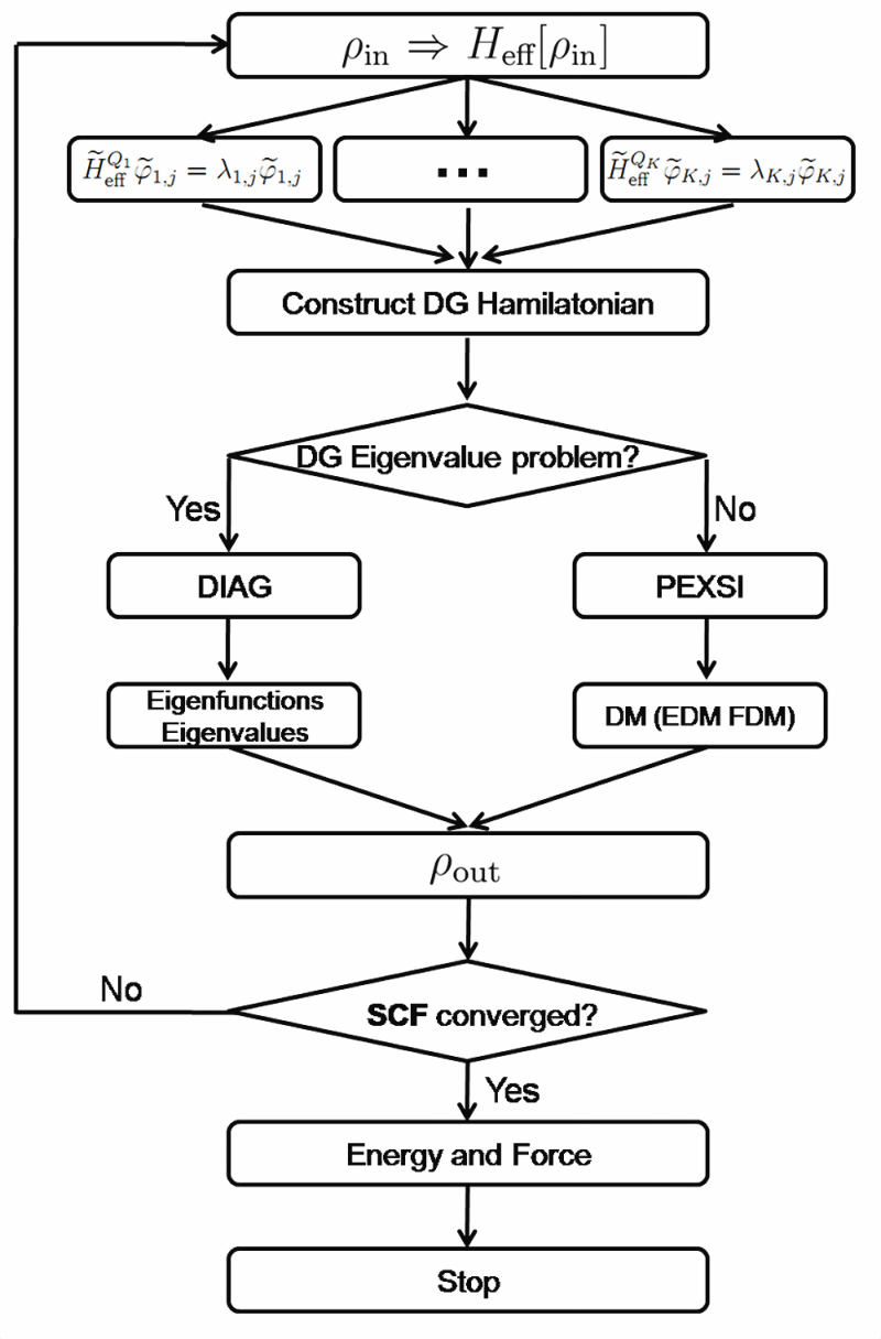
One notable feature of the ALB set is that they are generated on the fly, and is adaptive not only to the atomic but also the environmental information. In order to construct ALBs, we introduce, for each element , an extended element that contains and a buffer region surrounding . We define to be the restriction of the effective potential at the current SCF step to , and to be the restriction of the nonlocal potential to . These restricted potentials define a local Kohn-Sham linear eigenvalue problem on each extended element :
| (9) |
This linear eigenvalue problem can be discretized by using traditional basis sets such as plane waves and solved by an iterative method such as the locally optimal block preconditioned conjugate gradient (LOBPCG) method. We remark that SCF iterations need not and should not be performed within each element . The lowest eigenvalues and the corresponding eigenfunctions are computed on . We then restrict from to . The truncated vectors are not necessarily orthonormal. Therefore, we orthonormalize the set of truncated eigenvectors to obtain . We then set each to zero outside of , so that it defined over the entire domain, but is in general discontinuous across the boundary of . These functions constitute the ALB set that we use to represent the Kohn-Sham Hamiltonian. Because they satisfy the orthonormality condition (2), the overlap matrix corresponding to the ALB set is an identity matrix. Hence, no generalized eigenvalue problem with a potentially ill-conditioned overlap matrix need to be solved. For more details of the construction of ALBs, such as the restriction of the potential and the choice of boundary conditions for the local eigenvalue problem (9), we refer readers to Ref. [21].
As an example, Fig. 2 shows the ALBs of a 2D phosphorene monolayer with phosphorus atoms (P140). This is a two-dimensional system, and the global computational domain is partitioned into equal sized elements along the Y and Z directions, respectively. For instance, the extended element associated with the element contains elements , , , , , , and . We show the isosurfaces of the first three ALB functions for this element in Fig. 2(a)-(c). Each ALB function shown is strictly localized inside and is therefore discontinuous across the boundary of elements. On the other hand, each ALB function is delocalized across a few atoms inside the element since they are obtained from eigenfunctions of local Kohn-Sham Hamiltonian. Although the basis functions are discontinuous, the electron density is well-defined and is very close to be a continuous function in the global domain (Fig. 2(d)).

To summarize, the flowchart of the DGDFT method for solving Kohn-Sham DFT is shown in Fig. 3.
II.2 Two level parallelization strategy
The DGDFT framework naturally lends itself to a two level parallelization strategy. At the coarse grained level, we distribute work among different processors by elements. We call this level of concurrency the inter-element parallelization. Within each element, the eigenvalue solvers on each local (extended) domain and the construction of the DG Hamiltonian matrix can be further parallelized. This level of parallelization is called the intra-element parallelization. We use the Message Passing Interface (MPI) to handle data communication.

We assume that the total number of processors is , where is the number of elements, and is the number of processors assigned to each element. We partition these processors into a 2D logical processor grid following a column major order as shown in Fig. 4. We call this 2D processor grid the global processor grid to distinguish it from other processor grids employed in various parts of the massively parallel DGDFT method. Each row (column) communicator of this grid is called a global row (column) communicator. The processors with ranks to ( are in the -th global column processor group, and are assigned to element for intra-element parallelization. Similarly, the processors with ranks () are in the -th global row processor group. When a very large number of processors are used, it is important to avoid global all-to-all communication as much as possible in order to reduce communication cost and achieve parallel scalability. Therefore by dividing processors into column and row processor groups, we can restrict most of the communication within a global column or row group.
Based on the intra-element parallelization strategy to be detailed below, the maximum number of processors that can be effectively used for a single element depends on the number of basis functions to be generated on a single element, which is usually on the order of . It can be as large as a few hundreds. The level of concurrency that can be achieved in the inter-element parallelization is determined by the number of elements. The maximum number of processors that can be employed by DGDFT is therefore determined by the number of basis functions per element multiplied by the number of elements, which is equal to the dimension of the DG Hamiltonian matrix. For example, the P140 system contains 140 phosphorus atoms and is partitioned into 64 (8 8) elements. There are about 2 atoms in each element and we use 50 basis per element. The maximum number of processors that can be effectively used for this system is 3,600. For the 2D phosphorene test problems (P3500 and P14000) used in this work, we partition the phosphorene systems into 1,600 (40 40) and 6,400 (80 80) elements respectively. The maximum number of processors that can be effectively used for these systems are 80,000 and 320,000, respectively. Currently, we are often limited by the number of processors available on the existing high performance computers such as the Edison system at NERSC. The maximum number of processors we can use is 128,000.
Generation of the ALB functions
For each extended element, the computation of eigenfunctions for the local Kohn-Sham Hamiltonian can be parallelized in a way similar to the parallelization of a standard planewave based Kohn-Sham DFT solver. The local Kohn-Sham orbitals form a local dense matrix of dimension . Here is the number of ALBs to be computed, and is the total number of grid points required to represent each local Kohn-Sham orbital in the real space, which is determined from the kinetic energy cutoff by the following rule:
| (10) |
Here is the length of the extended element along the -th coordinate direction. The total number of grid points is . In a typical calculation and as shown in Fig. 5.

On each extended element, we use the LOBPCG method[32] to solve the local Kohn-Sham orbitals. The main operations involved in the LOBPCG solver are: 1) The application of the local Hamiltonian operator to . 2) Dense matrix-matrix multiplication of the form , where matrices have the same dimension as the Kohn-Sham orbitals . 3) Dense matrix-matrix multiplication of the form , where has the same dimension as , and is a small matrix on the order of . 4) The diagonalization of matrices of size using the Rayleigh-Ritz procedure. 5) The application of a preconditioner operator.
It should be noted that the these different types of operations require different data distribution and task parallelization strategies. Operation 1) requires applying the Laplacian operator via the Fast Fourier Transform (FFT), the local pseudopotential operator and the nonlocal pseudopotential operator to . This can be done easily if the orbitals (i.e., columns of ) are partitioned along the column direction (see Fig. 5 (a)). Since each processor holds all entries of an orbital, the FFT can be done in the same way as in a sequential implementation. We further assume that each processor associated with the extended element has a copy of the local pseudopotential , and the nonlocal pseudopotential . Therefore all operations described in 1) can be performed in the same way as those in a sequential implementation.
The most efficient way to parallelize operations 2) and 3) is to partition by row blocks as shown in Fig. 5 (b). This is because for operation 2), one can compute the matrix inner product of each block locally on each processor, and then use MPI_Allreduce among the processors to sum up local products of size . For operation 3), there is no communication at all if all processors have a local copy of the matrix. Partitioning by columns would incur more communication cost and make this part of the computation less scalable. Since in each LOBPCG iteration we apply the Hamiltonian operator to once, but perform matrix-matrix multiplication of operation type 2) and matrix-matrix multiplication of operation type 3), it is worthwhile to switch back and forth between a column partition and row partition of in between the first and other types of operations performed in each LOBPCG iteration. This can be achieved by using a MPI_Alltoallv call.
For operation 4), since is usually on the order of hundreds in practice, we solve the Rayleigh-Ritz problem and perform subspace diagonalization locally on each processor. Numerical experiments indicate that this sequential part usually takes around or less than 1 second.
Finally, in our implementation we use the preconditioner proposed in Ref. [33] to accelerate the convergence of LOBPCG. The preconditioner can be easily applied to different orbitals simultaneously without communication. Thus a column partition of is suitable for applying the preconditioner in parallel.
Once the Kohn-Sham orbitals are constructed through LOBPCG, they are restricted from the extended element to the element . After orthonormalizing columns of the restricted , we obtain the ALBs denoted by . We remark that it is not necessary to compute the local wavefunctions to full accuracy before the electron density becomes self consistent in the SCF iteration. As the accuracy of the electron density improves during the SCF cycle, a more accurate can be obtained from running a few iterations of the LOBPCG procedure that uses the returned from the previous SCF iteration as a starting guess. In practice, we find that using preconditioned LOBPCG iterations per SCF iteration is often sufficient to achieve rapid convergence of the SCF procedure. Our numerical results indicate that the overall procedure for generating the ALBs is highly efficient. For instance, for the phosphorene P3500 system, the total time for generating the ALBs is only 1.35 and 0.71 sec by using 12,800 and 25,600 processors, respectively.
Construction of the DG Hamiltonian
Due to the spatial locality of the ALBs, the DG Hamiltonian matrix in Eq. (5) is a sparse matrix and has a block structure that can be naturally distributed among different column processor groups assigned to different elements as shown in Fig. 1 (c), i.e. the processors assigned to the element assembles the -th block row of . The construction of the DG Hamiltonian matrix consists of the evaluation of volume integrals within each element and surface integrals at the boundary of different elements. To achieve high accuracy, all integrals in (5) are evaluated by a Gaussian quadrature defined on a Legendre-Gauss-Labotto (LGL) grid in each element. The gradients of ALBs sampled on the LGL grid points and denoted by , can be evaluated by applying differentiation matrices to along the directions, respectively. To compute efficiently, both and should be partitioned and distributed by columns among processors assigned to . We refer readers to e.g. Ref. [34] for details of constructing differentiation matrices associated with Gaussian quadratures.
The construction of the -th block row of consists of the following three steps that correspond to the three terms grouped by parentheses on the right hand side of Eq. (5). 1) Compute contributions to the diagonal matrix blocks from the kinetic energy and terms. 2) Compute contributions to the diagonal and off-diagonal matrix blocks from the nonlocal pseudopotential term. 3) Compute contributions to the diagonal and off-diagonal matrix blocks from the boundary integral terms.
In step 1), it is generally more efficient to partition columns of among different processors as shown in Fig. 5(a) because applying a differentiation matrix, or local pseudopotential to different columns of requires no communication. The inner products , however, are evaluated as vector inner products (or a matrix-matrix multiplication when several integrals are evaluated simultaneously). A block row partition is more efficient for these types of operations. Collective communication is required to sum up local products. To accommodate both data distribution schemes in this step, we use the MPI_Alltoallv call within a global column processor group to convert and from column partition to row partition.
More sophisticated data communication is needed for step 2. This is because the projection vector of a nonlocal pseudopotential may be distributed among several elements (up to 8, see Fig. 1 (b)). If the nonzero support of the projection operator is completely within one element , this projection operator only contributes to one diagonal block . Otherwise it contributes also to some off-diagonal matrix blocks for all ’s that contain a distributed portion of the projection vector. Unlike the local pseudopotential , the nonlocal pseudopotential does not need to be updated during the SCF iteration. Therefore, it is efficient for processors associated with the element to own a distributed portion of the projection vector on the LGL grid constructed on , if does not vanish on . This allows the inner product to be entirely evaluated on processors associated with without further inter-element communication. The computation of the matrix element however, requires data communication between processors associated with and , on which does not vanish. This is done by communicating the inner products of the form among such neighboring elements. Since the size of such inner products is independent of the LGL grid size, the communication volume of this step is relatively low. For inter-element parallelization, we use asynchronous data communication routines with MPI_Isend and MPI_Irecv for efficient data communication.
The boundary integrals that appear in step 3 also require inter-element communication. However, the inter-element data communication only occurs among two neighboring elements if the two elements share a common surface . It should be noted that the computation of average and jump operators only requires values of functions on the surface , and therefore only the function values of and together with their gradients and restricted to need to be computed. These calculations require much lower communication volume compared to those required in volume integrals. We also remark that the communication performed in this step can be overlapped with computation to further reduce the cost of communication. In particular, we first launch the communication needed to carry out step 3 before starting to perform the computational tasks in step 1, which does not require inter-element data communication.
Numerical results indicate that the overall procedure for constructing the DG Hamiltonian matrix is highly efficient. For instance, for the phosphorene P3500 system, the total wall clock time used to construct the DG Hamiltonian matrix is only 1.11 and 0.84 sec when the construction is carried out on 12,800 and 25,600 processors, respectively.
Computation of the electron density
As discussed in section II.1, the electron density can be assembled from the eigenvector coefficients , or from the diagonal matrix blocks of the density matrix directly. Both options are supported in DGDFT. When the eigenvector option is used, we diagonalize the DG Hamiltonian matrix (referred to as the ”DIAG” method) by using the ScaLAPACK software package.[35] In order to use ScaLAPACK, we need to convert the block row partition of the DG Hamiltonian matrix (see Fig. 1) to the 2D block cyclic data distribution scheme required by ScaLAPACK. The eigenvectors returned from ScaLAPACK, which are stored in the 2D block cyclic format, are redistributed according to the block row partition used to distribute . We developed a routine to perform these conversions. Such conversion is the only operation in DGDFT that involves MPI communication among, in principle, all the available processors. All other MPI communication is performed either within the global row processor group or the global column processor group. We note that a similar conversion procedure also can be found in other electronic structure software packages such as SIESTA[6] and CP2K[16] when ScaLAPACK is used.
Once the eigenvectors are redistributed by elements, the electron density can be evaluated locally on each element. The global electron density is imply the collection of the density defined on each local element. Such global electron density is never collected to be stored a single processor, but is distributed across processors in a global row processor group.
It should be noted that for large systems, all ScaLAPACK diagonalization routines (such as the divided and conquer routine PDSYEVD currently used in DGDFT) have limited parallel scalability. They often cannot make efficient use of the maximum number of processors (which can be or more) that can be used by other parts of the DGDFT calculation. Therefore, we often need to restrict the ScaLAPACK calculation to a subset of processors to avoid getting sub-optimal performance.
II.3 Pole expansion and selected inversion method
When the electron density is computed from the expression given in (8), we use the recently developed pole expansion and selected inversion (PEXSI) method[27, 28, 29] to compute the diagonal blocks of the density matrix. This technique avoids the diagonalization procedure which has an complexity. It is accurate for both insulating and metallic systems. Furthermore, the computational complexity of the PEXSI method is only for 1D systems, for 2D systems, and for 3D systems. Therefore, the PEXSI method is particularly well suited for studying electronic structures of larges scale low-dimensional (1D and 2D) systems.[36, 37]
The PEXSI method is based on approximating the density matrix by a linear combination of Green’s functions, i.e.,
| (11) |
where the integration weights and shifts are chosen carefully so that the number of expansion terms is proportional to , where is the inverse temperature and is the spectrum width of . In practical calculations, we observe that it is often sufficient to choose to be much smaller than the true spectrum width of , thanks to the exponential decay of the Fermi-Dirac function above the Fermi energy. In most cases, it is sufficient to choose . If we only need the diagonal blocks of the density matrix , we do not need to compute the entire inverse of . Only the diagonal blocks of need to be computed, and these diagonal blocks can be computed efficiently by using the selected inversion method.[27] The use of selected inversion leads to favorable complexity of the PEXSI method.
The PEXSI method can scale to to processors. This has recently been demonstrated in the massively parallel SIESTA-PEXSI method[29, 36]. SIESTA-PEXSI uses local atomic orbitals to discretize the Kohn-Sham Hamiltonian. Because DGDFT is designed to take advantage of massively parallel computers, the high scalability of PEXSI, in addition to its lower asymptotic complexity, makes it a more attractive option compared to the diagonalization option. When the PEXSI option is used, DGDFT can often scale to processors, and be used to solve the electronic structure problems with more than atoms efficiently.[37]
In order to use PEXSI in DGDFT, the DG Hamiltonian matrix needs to be redistributed from a block row distribution format to a distributed compressed sparse column format (DCSC). When the DCSC format is used to distribute a sparse Hamiltonian matrix among processors, each processor holds roughly columns stored in a compressed sparse column (CSC) format, where is the dimension of the matrix. The diagonal blocks of the density matrix returned from PEXSI, which are stored in DCSC format, are converted back to the block row partition format used to represent the electron density.
Because the selected inversions of the shifted DG Hamiltonians are independent of each other for different poles , we can carry out these selected inversions among different global row processor groups. Therefore, unlike the data redistribution scheme used for ScaLAPACK. As a result, the procedure for redistributing required by PEXSI uses asynchronous communication only within a global row processor group.
Because each parallel selected inversion requires processors to be arranged logically into a 2D grid of size (#PEXSIProcRow)(#PEXSIProcCol), the processors within each global row processor group is reconfigured in PEXSI as shown in Fig. 6. Note that restricting the selected inversion at each pole to processors belonging to a global processor row group limits the maximum number of processors that can be used for each selected inversion to the number of elements . However, for systems of large size, can be easily or more. Therefore such a configuration does not severely limit the number of processors that can be effectively used for selected inversion. If the number of processors () within each global column processors group is larger than the number of poles , all selected inversions required in the pole expansion (11) can be carried out simultaneously. The number of processors that can effectively be used in PEXSI is . If , we have to process at most poles at a time, and repeat the process until selected blocks of have been computed for all ’s. In this case and when all processors in a global processor row group are used for selected inversion, all processors can be effectively used by PEXSI.

III Computational results
In this section, we report the performance and accuracy of DGDFT when it is applied to 2D phosphorene systems of different sizes.
Phosphorene, a new two dimensional (2D) elemental monolayer,[38, 39, 40, 41, 42] has received considerable amount of interest recently after it has been experimentally isolated through mechanical exfoliation from bulk black phosphorus. Phosphorene exhibits some remarkable electronic properties superior to graphene, a well known elemental sp2-hybridized carbon monolayer.[43, 44, 45] For example, phosphorene is a direct semiconductor with a high hole mobility.[38] It has the drain current modulation up to 105 in nanoelectronics.[39] These remarkable properties have already been used for wide applications in field effect transistors[40] and thin-film solar cells.[41] Furthermore, up to now, phosphorene is the only stable elemental 2D material which can be mechanically exfoliated in experiments[38] besides graphene. Therefore, it can potentially be used as an alternative to graphene in the future and lead to faster semiconductor electronics.
Fig. 2 shows the atomic configuration of 2D phosphorene monolayer in a 5 7 supercell (P140). Other phosphorene models in very large supercells involving thousands or tens of thousands of atoms, such as the 25 35 (P3500) and 50 70 (P14000) supercells, which we use as test problems in this work, are not shown here. The vacuum space in the X and Y directions is about 10 Å to separate the interactions between neighboring slabs in phosphorene.
All calculations are performed on the Edison platform available at the National Energy Research Scientific Computing (NERSC) center. Edison has 5462 Cray XC30 nodes. Each node has 24 cores partitioned among two Intel Ivy Bridge processors. Each 12-core processor runs at 2.4GHz, and has 64 GB of memory per node. The maximum number of available cores is 131,088 on Edison. In all calculations, we utilize all cores on a computational node.
III.1 Computational accuracy
We use the conventional plane wave software package ABINIT[14] as a reference to check the accuracy of results from DGDFT. The same exchange-correlation functional of the local density approximation of Goedecker, Teter, Hutter (LDA-Teter93)[46] and the Hartwigsen-Goedecker-Hutter (HGH) norm-conserving pseudopotential[47] are adopted in both ABINIT and DGDFT software packages.
We first check the accuracy of the total energy and the atomic force of the DGDFT method by using P140 shown in Fig. 2 as an example. To simplify our discussion, we define the total energy error per atom E (Hartree/atom) and maximum atomic force error F (Hartree/Bohr) as
and
respectively, where is the total number of atoms. and represent the total energy computed by DGDFT and ABINIT respectively, and and represent the Hellmann-Feynman force on the -th phosphorus atom in P140 computed by DGDFT and ABINIT, respectively. The ABINIT results are obtained by setting the energy cutoff to 200 Hartree for the wavefunction to ensure full convergence. The kinetic energy cutoff (denoted by Ecut) in the DGDFT method is used to defined the grid size for computing the ALBs as is in standard Kohn-Sham DFT calculations using planewave basis sets. Ecut is also directly related to the Legendre-Gauss-Lobatto (LGL) integration grid defined on each element and used to perform numerical integration as needed to construct the DG Hamiltonian matrix. The number of LGL grids per direction is set to be twice the number of grid points calculated using Eq. (10) with the same Ecut.
Table 1 shows that the total energy and atomic forces produced by the DGDFT method are highly accurate compared to the ABINIT results. In particular, the total energy error can be as small as Hartree/atom if the DIAG method is used and Hartree/atom if the PEXSI method is used respectively. Here poles are used and the accuracy of PEXSI can be further improved by increasing the number of poles.The maximum error of the atomic force can be as small as Hartree/Bohr when DIAG is used and Hartree/Bohr when PEXSI is used. These results are obtained when only a relatively small number of ALB functions per atom are used to construct the global DG Hamiltonian. The energy cutoff for constructing the ALBs is set to 200 Hartree in this case. Note that the accuracy of total energy and atomic force in DGDFT depends on both the energy cutoff for local wavefunctions defined on an extended element and the number of ALB functions. We can see from Table 1 that the accuracy of the total energy and atomic forces both improve as the energy cutoff and the number of ALB functions increases. We also find that the use of the Hellmann-Feynman force can result in accurate force calculation, despite that the contribution from the Pulay force[48] is not included.
| DGDFT P140 | DIAG | PEXSI | |||
|---|---|---|---|---|---|
| Ecut | #ALB | ||||
| 20 | 91.43 | 5.22E-04 | 4.03E-03 | 3.22E-04 | 4.03E-03 |
| 40 | 18.28 | 4.51E-02 | 5.97E-02 | 4.57E-02 | 5.97E-02 |
| 40 | 27.42 | 6.67E-04 | 2.51E-03 | 6.85E-04 | 2.52E-03 |
| 40 | 36.57 | 1.34E-04 | 6.16E-04 | 1.59E-04 | 6.18E-04 |
| 40 | 45.71 | 7.00E-05 | 4.00E-04 | 6.44E-05 | 5.23E-04 |
| 40 | 91.43 | -4.32E-07 | 5.93E-04 | 1.34E-04 | 5.93E-04 |
| 100 | 91.43 | 1.59E-05 | 1.97E-04 | 8.04E-05 | 1.97E-04 |
| 200 | 91.43 | 3.39E-06 | 1.06E-04 | 8.12E-05 | 1.06E-04 |
In the following parallel efficiency tests, we set the energy cutoff to 40 Hartree for ALBs and 36.57 ALB functions per atom (80 ALB functions per element), which achieves good compromise between accuracy and computational efficiency. For this particular choice of the energy cutoff and the number of ALB functions, we are able to keep the total energy error under 1 10-4 Hartree/atom and atomic force error under 1 10-3 Hartree/Bohr for 2D phosphorene systems.
III.2 Parallel efficiency
To illustrate the parallel scalability of the DGDFT method, we demonstrate the performance of three main steps in each SCF iteration as shown in Fig. 3: (a) the generation of ALB functions, (b) the construction of DG Hamiltonian matrix and (c) the evaluation of the approximate charge density, energy and atomic forces by either diagonalizing the DG Hamiltonian (DIAG) or by using the PEXSI technique. Note that there are some additional steps such as the computation of energy, charge mixing or potential mixing, and intermediate data communication etc. The cost of these extra steps is included in the total wall clock time.
Fig. 7 shows the strong parallel scaling of these three individual steps, as well as the overall DGDFT method, for two large-scale 2D phosphorene monolayers (P3500 and P14000) in terms of the wall clock time per SCF step. For P3500, we tested the performance using both the DIAG and PEXSI methods for the evaluation of charge density during SCF. But for P14000, we only use the PEXSI method, since the DIAG method is too expensive for systems of such size (the dimension of the matrix is ).

The wall clock time of the first two steps are independent of whether PEXSI or DIAG is used. Fig. 7(a) and (b) show that they both scale well with respect to the number of cores used in the computation for all test problems we used. The exception is the construction of the DG Hamiltonian which does not scale beyond processors for P14000. We find that the only routine does not scale well is the inter-element communication of the boundary values of and , which is currently implemented via asynchronous communication. Since the volume of the asynchronous communication is proportional to the system size, for a large system the communication volume may exceed the size of the MPI buffer which leads to sub-optimal performance of the asynchronous data communication. Nonetheless, the cost of the generation of ALBs and the construction of the DG matrix is much less compared to that for computing the electron density from the DG Hamiltonian.
Fig. 7(c) and (d) show that the evaluation of the approximate charge density using the DG Hamiltonian matrix dominates the total wall clock time per SCF iteration in the DGDFT methodology for systems of large sizes. For large-scale 2D phosphorene systems P3500 and P14800, the PEXSI method can effectively reduce the wall clock time compared to the DIAG method in the DGDFT methodology. Furthermore, using the DIAG method with ScaLAPACK,[35] appears to limit the strong parallel scalability to at most 10,000 cores on the Edison. Increasing the cores beyond that can lead to an increase in wall clock time. In contrast, the PEXSI method exhibits highly scalable performance. It can make efficient use of about 100,000 cores on Edison for P3500 and P14000.
Fig. 8 shows the speedup and parallel efficiency with respect to the number of cores used for the computation for 2D phosphorene P3500 and P14000. For the P3500 system, both the DIAG and PEXSI methods in DGDFT can keep highly parallel efficiency (90% for DIAG and 80% for PEXSI) with less than 10,000 cores. But for the DIAG method, further increase of the number of cores will lead to rapid loss of parallel efficiency. On the contrary, the PEXSI method is highly scalable, and its parallel efficiency is about 80% even when the number of cores increases beyond 80,000 for the P3500 system. For the large-scale P14000 system, we only use the PEXSI method in DGDFT, and we find that the parallel efficiency of the DGDFT-PEXSI method around 80% when 128,000 cores are used on Edison (Edison has cores in total).

IV Conclusions
We described a massively parallel implementation of the DGDFT (Discontinuous Galerkin Density Functional Theory) methodology that can be used to perform large-scale Kohn-Sham density functional theory (DFT) calculations efficiently. We demonstrated the accuracy and efficiency of our parallel implementation. In particular, we showed that DGDFT can achieve accuracy comparable to that produced by a conventional planewave based calculation with far fewer number of basis functions. We also showed that DGDFT can efficiently use 128,000 computational cores to solve a problem with over atoms. The high parallel efficiency results from a two-level parallelization schemes that make use of several different types of data distribution, task scheduling and data communication schemes. It also benefits from the use of the PEXSI method to compute electron density, energy and atomic forces. The PEXSI method has a favorable computational complexity and is also amenable to a two-level parallelization scheme that enables it to achieve high parallel efficiency.
V Acknowledgement
This work is partially supported by the Scientific Discovery through Advanced Computing (SciDAC) Program funded by U.S. Department of Energy, Office of Science, Advanced Scientific Computing Research and Basic Energy Sciences (W. H., L. L. and C. Y.), and by the Center for Applied Mathematics for Energy Research Applications (CAMERA), which is a partnership between Basic Energy Sciences and Advanced Scientific Computing Research at the U.S Department of Energy (L. L. and C. Y.). We thank the National Energy Research Scientific Computing (NERSC) center for the computational resources.
References
- [1] P. Hohenberg and W. Kohn, Phys. Rev. 136, B864 (1964).
- [2] W. Kohn and L. J. Sham, Phys. Rev. 140, B1133 (1965).
- [3] S. Goedecker, Rev. Mod. Phys. 71, 1085 (1999).
- [4] H. Shang, H. Xiang, Z. Li, and J. Yang, Int. Rev. Phys. Chem. 29, 665 (2010).
- [5] D. R. Bowler and T. Miyazaki, Rep. Prog. Phys. 75, 036503 (2012).
- [6] J. M. Soler, E. Artacho, J. D. Gale, A. García, J. Junquera, P. Ordejón, and D. Sánchez-Portal, J. Phys.: Condens. Matter 14, 2745 (2002).
- [7] T. Ozaki and H. Kino, Phys. Rev. B 72, 045121 (2005).
- [8] X. Qin, H. Shang, H. Xiang, Z. Li, and J. Yang, Int. J. Quantum Chem. 115, 647 (2014).
- [9] J. VandeVondele, M. Krack, F. Mohamed, M. Parrinello, T. Chassaing, and J. Hutter, Comput. Phys. Commun. 167, 103 (2005).
- [10] M. J. Gillan, D. R. Bowler, A. S. Torralba, and T. Miyazaki, Comput. Phys. Commun. 177, 14 (2007).
- [11] G. Kresse and J. Furthmüller, Phys. Rev. B 54, 11169 (1996).
- [12] G. Kresse and J. Hafner, Phys. Rev. B 47, 558(R) (1993).
- [13] P. Giannozzi, S. Baroni, N. Bonini, M. Calandra, R. Car, C. Cavazzoni, D. Ceresoli, G. L. Chiarotti, M. Cococcioni, I. Dabo, et al., J. Phys.: Condens. Matter 21, 395502 (2009).
- [14] X. Gonze, B. Amadon, P.-M. Anglade, J.-M. Beuken, F. Bottin, P. Boulanger, F. Bruneval, D. Caliste, R. Caracas, M. Côté, et al., Comput. Phys. Commun. 180, 2582 (2009).
- [15] F. Gygi, IBM J. Res. Dev. 52, 1 (2008).
- [16] J. VandeVondele, U. Bors̆tnik, and J. Hutter, J. Chem. Theory Comput. 8, 3565 (2012).
- [17] D. R. Bowler and T. Miyazaki, J. Phys.: Condens. Matter 22, 074207 (2010).
- [18] C. Saravanan, Y. Shao, R. Baer, P. N. Ross, and M. Head¨CGordon, J. Comput. Chem. 24, 618 (2003).
- [19] E. H. Rubensson and E. Rudberg, J. Comput. Chem. 32, 1411 (2011).
- [20] U. Bors̆tnik, J. VandeVondele, V. Weber, and J. Hutter, Parallel Comput. 40, 47 (2014).
- [21] L. Lin, J. Lu, L. Ying, and W. E, J. Comput. Phys. 231, 2140 (2012).
- [22] C. K. Skylaris, P. D. Haynes, A. A. Mostofi, and M. C. Payne, J. Chem. Phys. 122, 084119 (2005).
- [23] S. Mohr, L. E. Ratcliff., P. Boulanger, L. Genovese, D. Caliste, T. Deutsch, and S. Goedecker, J. Chem. Phys. 140, 204110 (2014).
- [24] D. N. Arnold, SIAM J. Numer. Anal. 19, 742 (1982).
- [25] D. N. Arnold, F. Brezzi, B. Cockburn, and L. D. Marini, SIAM J. Numer. Anal. 39, 1749 (2002).
- [26] J. Kaye, L. Lin, and C. Yang, Comm. Math. Sci. Accepted (2015).
- [27] L. Lin, J. Lu, L. Ying, R. Car, and W. E, Comm. Math. Sci. 7, 755 (2009).
- [28] L. Lin, M. Chen, C. Yang, and L. He, J. Phys.: Condens. Matter 25, 295501 (2013).
- [29] L. Lin, A. García, G. Huhs, and C. Yang, J. Phys.: Condens. Matter 26, 305503 (2014).
- [30] G. Zhang, L. Lin, W. Hu, C. Yang, and J. E. Pask, in preparation (2015).
- [31] L. Kleinman and D. M. Bylander, Phys. Rev. Lett. 48, 1425 (1982).
- [32] A. V. Knyazev, SIAM J. Sci. Comp. 23, 517 (2001).
- [33] M. C. Payne, M. P. Teter, D. C. Allen, T. A. Arias, and J. D. Joannopoulos, Rev. Mod. Phys. 64, 1045 (1992).
- [34] L. N. Trefethen, Spectral methods in MATLAB, vol. 10 (SIAM, 2000).
- [35] T. Auckenthaler, V. Blum, H. J. Bungartz, T. Huckle, R. Johanni, L. Krämer, B. Lang, H. Lederer, and P. R. Willems, Parallel Comput. 37, 783 (2011).
- [36] W. Hu, L. Lin, C. Yang, and J. Yang, J. Chem. Phys. 141, 214704 (2014).
- [37] W. Hu, L. Lin, and C. Yang, Phys. Chem. Chem. Phys. Accepted (2015a).
- [38] H. Liu, A. T. Neal, Z. Zhu, Z. Luo, X. Xu, D. Tománek, and P. D. Ye, ACS Nano 8, 4033 (2014).
- [39] J. Qiao, X. Kong, Z.-X. Hu, F. Yang, and W. Ji, Nature Commun. 5, 4475 (2014).
- [40] L. Li, Y. Yu, G. Ye, Q. Ge, X. Ou, H. Wu, D. Feng, X. Chen, and Y. Zhang, Nature Nanotech. 9, 372 (2014).
- [41] J. Dai and X. C. Zeng, J. Phys. Chem. Lett. 5, 1289 (2014).
- [42] W. Hu, T. Wang, and J. Yang, J. Mater. Chem. C 3, 4756 (2015b).
- [43] K. S. Novoselov, A. K. Geim, S. V. Morozov, D. Jiang, Y. Zhang, S. V. Dubonos, I. V. Grigorieva, and A. A. Firsov, Scinece 306, 666 (2004).
- [44] A. K. Geim and K. S. Novoselov, Nature Mater. 6, 183 (2007).
- [45] A. H. C. Neto, F. Guinea, N. M. R. Peres, K. S. Novoselov, and A. K. Geim, Rev. Mod. Phys. 18, 109 (2009).
- [46] S. Goedecker, M. Teter, and J. Hutter, Phys. Rev. B 54, 1703 (1996).
- [47] C. Hartwigsen, S. Goedecker, and J. Hutter, Phys. Rev. B 58, 3641 (1998).
- [48] P. Pulay, Chem. Phys. Lett. 73, 393 (1980).