A feasible second order bundle algorithm for nonsmooth nonconvex optimization problems with inequality constraints: II. Implementation and numerical results

Hannes Fendl ^†^†thanks: This research was supported by the Austrian Science Found (FWF) Grant Nr.˜P22239-N13. Hermann Schichl E-mail: hermann.schichl@univie.ac.at Affiliation: Faculty of Mathematics, University of Vienna, Austria
Oskar-Morgenstern-Pl. 1, A-1090 Wien, Austria

Abstract

This paper presents a concrete implementation of the feasible second order bundle algorithm for nonsmooth, nonconvex optimization problems with inequality constraints Fendl & Schichl (2011). It computes the search direction by solving a convex quadratically constrained quadratic program. Furthermore, certain versions of the search direction problem are discussed and the applicability of this approach is justified numerically by using different solvers for the computation of the search direction. Finally, the good performance of the second order bundle algorithm is demonstrated by comparison with test results of other solvers on examples of the Hock-Schittkowski collection, on custom examples that arise in the context of finding exclusion boxes for quadratic constraint satisfaction problems, and on higher dimensional piecewise quadratic examples.

Keywords:

Nonsmooth optimization, nonconvex optimization, bundle method

MSC

90C56, 49M37, 90C30

1 Introduction

Nonsmooth optimization addresses to solve the optimization problem

\begin{split}&\min{f(x)}\\ &\textnormal{ s.t. }F_{i}(x)\leq 0\penalty\ \penalty\ \penalty\ \textnormal{for all }i=1,\dots,m\textnormal{\penalty\ ,}\end{split}

(1)

where $f,F_{i}:\mathbb{R}^{n}\longrightarrow\mathbb{R}$ are locally Lipschitz continuous. Since $F_{i}(x)\leq 0$ for all $i=1,\dots,m$ if and only if $F(x):=\max_{i=1,\dots,m}{c_{i}F_{i}(x)}\leq 0$ with constants $c_{i}>0$ and since $F$ is still locally Lipschitz continuous (cf., e.g., Mifflin (1977, p. 969, Theorem 6 (a))), we can always assume $m=1$ in (1). Therefore w.l.o.g. we always consider the nonsmooth optimization problem with a single nonsmooth constraint

\begin{split}&\min{f(x)}\\ &\textnormal{ s.t. }F(x)\leq 0\textnormal{\penalty\ ,}\end{split}

(2)

where $F:\mathbb{R}^{n}\longrightarrow\mathbb{R}$ is locally Lipschitz continuous.

Since locally Lipschitz continuous functions are differentiable almost everywhere, both $f$ and $F$ may have kinks and therefore already the attempt to solve an unconstrained nonsmooth optimization problem by a smooth solver (e.g., by a line search algorithm or by a trust region method) by just replacing the gradient by a subgradient, fails in general (cf., e.g., Zowe (1989, p. 461-462)): If $g$ is an element of the subdifferential $\partial f(x)$ , then the search direction $-g$ does not need to be a direction of descent (contrary to the behavior of the gradient of a differentiable function). Furthermore, it can happen that $\{x_{k}\}$ converges towards a minimizer $\hat{x}$ , although the sequence of gradients $\{\nabla f(x_{k})\}$ does not converge towards $0$ and therefore we cannot identify $\hat{x}$ as a minimizer. Moreover, it can happen that $\{x_{k}\}$ converges towards a point $\hat{x}$ , but $\hat{x}$ is not stationary for $f$ . The reason for these problems is that if $f$ is not differentiable at $x$ , then the gradient $\nabla f$ is discontinuous at $x$ and therefore $\nabla f(x)$ does not give any information about the behavior of $\nabla f$ in a neighborhood of $x$ .

Not surprisingly, like in smooth optimization, the presence of constraints adds additional complexity, since constructing a descent sequence whose limit satisfies the constraints is (both theoretically and numerically) much more difficult than achieving this aim without the requirement of satisfying any restrictions.
Linearly constrained nonsmooth optimization. There exist various types of nonsmooth solvers like, e.g., the R-algorithm by Shor (1985) or stochastic algorithms that try to approximate the subdifferential (e.g., by Burke et al. (2005)) or bundle algorithms which force a descent of the objective function by using local knowledge of the function. We will concentrate on the latter ones as they proved to be quite efficient.

One of the few publicly available bundle methods is the bundle-Newton method for nonsmooth, nonconvex unconstrained minimization by Lukšan & Vlček (1998). We sum up its key features: It is the only method which we know of that uses second order information of the objective function, which results in faster convergence (in particular it was shown in Lukšan & Vlček (1998, p. 385, Section 4) that the bundle-Newton method converges superlinearly for strongly convex functions). Furthermore, the search direction is computed by solving a convex quadratic program (QP) (based on an SQP-approach in some sense) and it uses a line search concept for deciding whether a serious step or a null step is performed. Moreover, its implementation PNEW, which is described in Lukšan & Vlček (1997), is written in FORTRAN. Therefore, we can use the bundle-Newton method for solving linearly constrained nonsmooth optimization problems (as the linear constraints can just be inserted into the QP without any additional difficulties).

In general, every nonsmooth solver for unconstrained optimization can treat constrained problems via penalty functions. Nevertheless, choosing the penalty parameter well is a highly nontrivial task. Furthermore, if an application only allows the nonsmooth solver to perform a few steps (as, e.g., in Fendl et al. (2011, )), we need to achieve a feasible descent within these steps.

Nonlinearly constrained nonsmooth optimization. Therefore, Fendl & Schichl (2011, ) give an extension of the bundle-Newton method to the constrained case in a very special way: We use second order information of the constraint (cf. (2)). Furthermore, we use the SQP-approach of the bundle-Newton method for computing the search direction for the constrained case and combine it with the idea of quadratic constraint approximation, as it is used, e.g., in the sequential quadratically constrained quadratic programming method by Solodov (2004) (this method is not a bundle method), in the hope to obtain good feasible iterates, where we only accept strictly feasible points as serious steps. Therefore, we have to solve a strictly feasible convex QCQP for computing the search direction. Using such a QCQP for computing the search direction yields a line search condition for accepting infeasible points as trial points (which is different to that in, e.g., Mifflin (1982)). One of the most important properties of the convex QP (that is used to determine the search direction) with respect to a bundle method is its strong duality (e.g., for a meaningful termination criterion, for global convergence,…) which is also true in the case of strictly feasible convex QCQPs (cf. Fendl & Schichl (2011, )). Since there exist only a few solvers specialized in solving QCQPs (all written in MATLAB or C, none in FORTRAN), the method is implemented in MATLAB as well as in C.

For a detailed description of the presented issues we refer the reader to Fendl (2011, ).

The paper is organized as follows: In Section 2 we give a brief description of the implemented variant of the second order bundle algorithm. In Section 3 we discuss some aspects that arise when using a convex QCQP for the computation of the search direction problem like the reduction of its dimension and the existence of a strictly feasible starting point for its SOCP-reformulation. Furthermore, we justify the approach for determining the search direction by solving a QCQP numerically by comparing the results of some well-known solvers for our search direction problem. In Section 4 we provide numerical results for our second order bundle algorithm for some examples of the Hock-Schittkowski collection by Schittkowski (2009a); Schittkowski (2009b), for custom examples that arise in the context of finding exclusion boxes for a quadratic CSP (constraint satisfaction problem) in GloptLab by Domes (2009) as well as for higher dimensional piecewise quadratic examples, and finally we compare these results to those of MPBNGC by Mäkelä (2003) and SolvOpt by Kappel & Kuntsevich (2000) to emphasize the good performance of the algorithm on constrained problems.

Throughout the paper we use the following notation: We denote the non-negative real numbers by $\mathbb{R}_{\geq 0}:=\{x\in\mathbb{R}:\penalty\ x\geq 0\}$ , and the space of all symmetric $n\times n$ -matrices by $\mathbb{R}_{\mathrm{sym}}^{n\times n}$ . For $x\in\mathbb{R}^{n}$ we denote the Euclidean norm of $x$ by $\lvert x\rvert$ , for $1\leq i\leq j\leq n$ we define the (MATLAB-like) colon operator $x_{i:j}:=(x_{i},\dots x_{j})$ , and for $A\in\mathrm{Sym(n)}$ we denote the spectral norm of $A$ by $\lvert A\rvert$ .

2 Presentation of the algorithm

In the following section we give a brief exposition of our implemented variant of the second order bundle algorithm whose theoretical convergence properties are proved in Fendl & Schichl (2011). For this purpose we assume that the functions $f,F:\mathbb{R}^{n}\longrightarrow\mathbb{R}$ are locally Lipschitz continuous, that $g_{j}\in\partial f(y_{j})$ and $\hat{g}_{j}\in\partial F(y_{j})$ , and $G_{j}\in\partial^{2}{f}{(y_{j})}$ , $\hat{G}_{j}\in\partial^{2}{F}{(y_{j})}$ , where the set $\partial^{2}{f}{(x)}\subseteq\mathbb{R}_{\mathrm{sym}}^{n\times n}$ of the substitutes for the Hessian of $f$ at $x$ is defined by

\partial^{2}{f}{(x)}:=\left\{\begin{array}[]{ll}\{G\}&\textnormal{if the Hessian }G\textnormal{ of }f\textnormal{ at }x\textnormal{ exists}\\ \mathbb{R}_{\mathrm{sym}}^{n\times n}&\textnormal{otherwise}\textnormal{\penalty\ ,}\end{array}\right.

i.e., we calculate elements of the sets $\partial^{2}{f}{(y)}$ and $\partial^{2}{F}{(y)}$ (in the proof of convergence in Fendl & Schichl (2011) only approximations were required). We consider the nonsmooth optimization problem (2) which has a single nonsmooth constraint. Then the second order bundle algorithm (described in Algorithm 2.1) tries to solve optimization problem (2) according to the following scheme: After choosing a starting point $x_{1}\in\mathbb{R}^{n}$ and setting up a few positive definite matrices, we compute the localized approximation errors. Then we solve a convex QCQP to determine the search direction, where the intention of the usage of the quadratic constraints of the QCQP is to obtain preferably feasible points that yield a good descent. Therefore, we only use quadratic terms in the QCQP for the approximation of the constraint, but not for the approximation of the objective function (in contrast to Fendl & Schichl (2011, )) to balance the effort of solving the QCQP with the higher number of iterations caused by this simplification (in Subsection 3.1 we will even discuss a further reduction of the size of the QCQP). Now, after computing the aggregated data and the predicted descent as well as testing the termination criterion, we perform a line search (s. Algorithm 2.2) on the ray given by the search direction which yields a trial point $y_{k+1}$ that has the following property: Either $y_{k+1}$ is strictly feasible and the objective function achieves sufficient descent (serious step) or $y_{k+1}$ is strictly feasible and the model of the objective function changes sufficiently (null step with respect to the objective function) or $y_{k+1}$ is not strictly feasible and the model of the constraint changes sufficiently (null step with respect to the constraint). Afterwards we update the iteration point $x_{k+1}$ and the information which is stored in the bundle. Now, we repeat this procedure until the termination criterion is satisfied.

Algorithm 2.1

Initialization:

Choose the following parameters, which will not be changed during the algorithm:

Table 1: Initial parameters

General	Default	Description
$x_{1}\in\mathbb{R}^{n}$		Strictly feasible initial point
$y_{1}=x_{1}$		Initial trial point
$\varepsilon\geq 0$		Final optimality tolerance
$M\geq 2$	$M=n+3$	Maximal bundle dimension
$t_{0}\in(0,1)$	$t_{0}=0.001$	Initial lower bound for step size
		of serious step in line search
$\hat{t}_{0}\in(0,1)$	$\hat{t}_{0}=0.001$	Scaling parameter for $t_{0}$
$m_{L}\in(0,\tfrac{1}{2})$	$m_{L}=0.01$	Descent parameter for serious step in line search
$m_{R}\in(m_{L},1)$	$m_{R}=0.5$	Parameter for change of model of objective function
		for short serious and null steps in line search
$m_{F}\in(0,1)$	$m_{F}=0.01$	Parameter for change of model of constraint
		for short serious and null steps in line search
$\zeta\in(0,\tfrac{1}{2})$	$\zeta=0.01$	Coefficient for interpolation in line search
$\vartheta\geq 1$	$\vartheta=1$	Exponent for interpolation in line search
$C_{S}>0$	$C_{S}=10^{50}$	Upper bound of the distance between $x_{k}$ and $y_{k}$
$C_{G}>0$	$C_{G}=10^{50}$	Upper bound of the norm of the damped
		matrices $\{\rho_{j}G_{j}\}$ ( $\lvert\rho_{j}G_{j}\rvert\leq C_{G}$ )
$\hat{C}_{G}>0$	$\hat{C}_{G}=C_{G}$	Upper bound of the norm of the damped
		matrices $\{\hat{\rho}_{j}\hat{G}_{j}\}$ ( $\lvert\hat{\rho}_{j}\hat{G}_{j}\rvert\leq\hat{C}_{G}$ )
$\bar{\hat{C}}_{G}>0$	$\bar{\hat{C}}_{G}=C_{G}$	Upper bound of the norm of the matrices
		$\{\bar{\hat{G}}_{j}^{k}\}$ and $\{\bar{\hat{G}}^{k}\}$ ( $\max{(\lvert\bar{\hat{G}}_{j}^{k}\rvert,\lvert\bar{\hat{G}}^{k}\rvert)}\leq\bar{\hat{C}}_{G}$ )
$i_{\rho}\geq 0$	$i_{\rho}=3$	Selection parameter for $\rho_{k+1}$
$i_{m}\geq 0$		Matrix selection parameter
$i_{r}\geq 0$		Bundle reset parameter
$\gamma_{1}>0$	$\gamma_{1}=1$	Coefficient for locality measure for objective function
$\gamma_{2}>0$	$\gamma_{2}=1$	Coefficient for locality measure for constraint
$\omega_{1}\geq 1$	$\omega_{1}=2$	Exponent for locality measure for objective function
$\omega_{2}\geq 1$	$\omega_{2}=2$	Exponent for locality measure for constraint

Set the initial values of the data which gets changed during the algorithm:

	$\displaystyle i_{n}$	$\displaystyle=\hphantom{\{}0\hphantom{\}}\textnormal{ (\# subsequent null and short steps)}$
	$\displaystyle i_{s}$	$\displaystyle=\hphantom{\{}0\hphantom{\}}\textnormal{ (\# subsequent serious steps)}$
	$\displaystyle J_{1}$	$\displaystyle=\{1\}\textnormal{ (set of bundle indices)}\textnormal{\penalty\ .}$

Compute the following information at the initial trial point

	$\displaystyle f_{p}^{1}=f_{1}^{1}$	$\displaystyle=f(y_{1})$
	$\displaystyle g_{p}^{1}=g_{1}^{1}$	$\displaystyle=g(y_{1})\in\partial f(y_{1})$
	$\displaystyle G_{p}^{1}=G_{1}$	$\displaystyle=G(y_{1})\in\partial^{2}{f}{(y_{1})}$
	$\displaystyle F_{p}^{1}=F_{1}^{1}$	$\displaystyle=F(y_{1})<0\penalty\ \penalty\ \penalty\ \textnormal{(}y_{1}\textnormal{ is strictly feasible according to assumption)}$
	$\displaystyle\hat{g}_{p}^{1}=\hat{g}_{1}^{1}$	$\displaystyle=\hat{g}(y_{1})\in\partial F(y_{1})$
	$\displaystyle\hat{G}_{p}^{1}=\hat{G}_{1}$	$\displaystyle=\hat{G}(y_{1})\in\partial^{2}{F}{(y_{1})}$

and set

	$\displaystyle\hat{s}_{p}^{1}=s_{p}^{1}=s_{1}^{1}$	$\displaystyle=0\textnormal{ (locality measure)}$
	$\displaystyle\hat{\rho}_{1}=\rho_{1}$	$\displaystyle=1\textnormal{ (damping parameter)}$
	$\displaystyle\bar{\kappa}^{1}$	$\displaystyle=1\textnormal{ (Lagrange multiplier for optimality condition)}$
	$\displaystyle k$	$\displaystyle=1\textnormal{ (iterator)}\textnormal{\penalty\ .}$

Determination of the matrices for the QCQP:

if (step $k-1$ and $k-2$ were serious steps) $\wedge$ ( $\lambda_{k-1}^{k-1}=1$ $\vee$ $\underset{\textnormal{bundle reset}}{\underbrace{i_{s}>i_{r}}}$ )
aaa $W=G_{k}+\bar{\kappa}^{k}\hat{G}_{k}$
else
aaa $W=G_{p}^{k}+\bar{\kappa}^{k}\hat{G}_{p}^{k}$
end

if $i_{n}\leq i_{m}$
aaa $\makebox[0.0pt][l]{\hskip 1.62497pt\hskip 0.0pt\hskip 4.73335pt\makebox[0.0pt][c]{\rule[8.12498pt]{6.97174pt}{0.43057pt}}}{W}_{p}^{k}=\textnormal{``positive definite modification of }W\textnormal{''}$
else
aaa $\makebox[0.0pt][l]{\hskip 1.62497pt\hskip 0.0pt\hskip 4.73335pt\makebox[0.0pt][c]{\rule[8.12498pt]{6.97174pt}{0.43057pt}}}{W}_{p}^{k}=\makebox[0.0pt][l]{\hskip 1.62497pt\hskip 0.0pt\hskip 4.73335pt\makebox[0.0pt][c]{\rule[8.12498pt]{6.97174pt}{0.43057pt}}}{W}_{p}^{k-1}$
end
Compute

\begin{split}(\makebox[0.0pt][l]{\hskip 1.70274pt\hskip 0.0pt\hskip 2.05557pt\makebox[0.0pt][c]{\rule[8.5139pt]{3.75839pt}{0.43057pt}}}{\hat{G}}^{k},\makebox[0.0pt][l]{\hskip 1.70274pt\hskip 0.0pt\hskip 2.05557pt\makebox[0.0pt][c]{\rule[8.5139pt]{3.75839pt}{0.43057pt}}}{\hat{G}}_{j}^{k})=\textnormal{``positive definite modification of }(\hat{G}_{p}^{k},\hat{G}_{j})\textnormal{''}\penalty\ \textnormal{for all }j\in J_{k}\textnormal{\penalty\ .}\end{split}

(3)

Computation of the localized approximation errors:

	$\displaystyle\alpha_{j}^{k}$	$\displaystyle:=\max{\big(\lvert f(x_{k})-f_{j}^{k}\rvert,\gamma_{1}(s_{j}^{k})^{\omega_{1}}\big)}\textnormal{\penalty\ ,}\quad\alpha_{p}^{k}:=\max\big(\lvert f(x_{k})-f_{p}^{k}\rvert,\gamma_{1}(s_{p}^{k})^{\omega_{1}}\big)$
	$\displaystyle A_{j}^{k}$	$\displaystyle:=\max{\big(\lvert F(x_{k})-F_{j}^{k}\rvert,\gamma_{2}(s_{j}^{k})^{\omega_{2}}\big)}\textnormal{\penalty\ ,}\quad A_{p}^{k}:=\max\big(\lvert F(x_{k})-F_{p}^{k}\rvert,\gamma_{2}(\hat{s}_{p}^{k})^{\omega_{2}}\big)\textnormal{\penalty\ .}$

Determination of the search direction: Compute the solution $(d_{k},\hat{v}_{k})\in\mathbb{R}^{n+1}$ of the (convex) QCQP

\begin{split}&\min_{d,\hat{v}}\hat{v}+\tfrac{1}{2}d^{T}\makebox[0.0pt][l]{\hskip 1.62497pt\hskip 0.0pt\hskip 4.73335pt\makebox[0.0pt][c]{\rule[8.12498pt]{6.97174pt}{0.43057pt}}}{W}_{p}^{k}d\textnormal{\penalty\ ,}\\ &\textnormal{ s.t. }-\alpha_{j}^{k}+d^{T}g_{j}^{k}\leq\hat{v}\penalty\ \penalty\ \hskip 82.0pt\textnormal{for }j\in J_{k}\\ &\hphantom{\textnormal{ s.t. }}-\alpha_{p}^{k}+d^{T}g_{p}^{k}\leq\hat{v}\penalty\ \penalty\ \hskip 82.0pt\textnormal{if }i_{s}\leq i_{r}\\ &\hphantom{\textnormal{ s.t. }}F(x_{k})-A_{j}^{k}+d^{T}\hat{g}_{j}^{k}+\tfrac{1}{2}d^{T}\makebox[0.0pt][l]{\hskip 1.70274pt\hskip 0.0pt\hskip 2.05557pt\makebox[0.0pt][c]{\rule[8.5139pt]{3.75839pt}{0.43057pt}}}{\hat{G}}_{j}^{k}d\leq 0\penalty\ \penalty\ \textnormal{for }j\in J_{k}\\ &\hphantom{\textnormal{ s.t. }}F(x_{k})-A_{p}^{k}+d^{T}\hat{g}_{p}^{k}+\tfrac{1}{2}d^{T}\makebox[0.0pt][l]{\hskip 1.70274pt\hskip 0.0pt\hskip 2.05557pt\makebox[0.0pt][c]{\rule[8.5139pt]{3.75839pt}{0.43057pt}}}{\hat{G}}^{k}d\leq 0\penalty\ \penalty\ \textnormal{if }i_{s}\leq i_{r}\end{split}

(4)

and its corresponding Lagrange multiplier $(\lambda^{k},\lambda_{p}^{k},\mu^{k},\mu_{p}^{k})\in\mathbb{R}_{\geq 0}^{2(\lvert J_{k}\rvert+1)}$ and set $H_{k}:=\big(\makebox[0.0pt][l]{\hskip 1.62497pt\hskip 0.0pt\hskip 4.73335pt\makebox[0.0pt][c]{\rule[8.12498pt]{6.97174pt}{0.43057pt}}}{W}_{p}^{k}+\sum_{j\in J_{k}}\mu_{j}^{k}\makebox[0.0pt][l]{\hskip 1.70274pt\hskip 0.0pt\hskip 2.05557pt\makebox[0.0pt][c]{\rule[8.5139pt]{3.75839pt}{0.43057pt}}}{\hat{G}}_{j}^{k}+\mu_{p}^{k}\makebox[0.0pt][l]{\hskip 1.70274pt\hskip 0.0pt\hskip 2.05557pt\makebox[0.0pt][c]{\rule[8.5139pt]{3.75839pt}{0.43057pt}}}{\hat{G}}^{k}\big)^{-\frac{1}{2}}$ and $\bar{\kappa}^{k+1}:=\sum_{j\in J_{k}}\mu_{j}^{k}+\mu_{p}^{k}$ .
if $\bar{\kappa}^{k+1}>0$
aaa $(\kappa_{j}^{k},\kappa_{p}^{k})=\tfrac{1}{\bar{\kappa}^{k+1}}(\mu_{j}^{k},\mu_{p}^{k})$
else
aaa $(\kappa_{j}^{k},\kappa_{p}^{k})=0$
end
if $i_{s}>i_{r}$
aaa $i_{s}=0$ (bundle reset)
end

Aggregation: We set for the aggregation of information of the objective function

	$\displaystyle(\tilde{f}_{p}^{k},\tilde{g}_{p}^{k},G_{p}^{k+1},\tilde{s}_{p}^{k})$	$\displaystyle=\sum\limits_{j\in J_{k}}\lambda_{j}^{k}(f_{j}^{k},g_{j}^{k},\rho_{j}G_{j},s_{j}^{k})+\lambda_{p}^{k}(f_{p}^{k},g_{p}^{k},G_{p}^{k},s_{p}^{k})$
	$\displaystyle\tilde{\alpha}_{p}^{k}$	$\displaystyle=\max\big(\|f(x_{k})-\tilde{f}_{p}^{k}\|,\gamma_{1}(\tilde{s}_{p}^{k})^{\omega_{1}}\big)$

and for the aggregation of information of the constraint

	$\displaystyle(\tilde{F}_{p}^{k},\tilde{\hat{g}}_{p}^{k},\hat{G}_{p}^{k+1},\tilde{\hat{s}}_{p}^{k})$	$\displaystyle=\sum\limits_{j\in J_{k}}\kappa_{j}^{k}(F_{j}^{k},\hat{g}_{j}^{k},\hat{\rho}_{j}\hat{G}_{j},s_{j}^{k})+\kappa_{p}^{k}(F_{p}^{k},\hat{g}_{p}^{k},\hat{G}_{p}^{k},\hat{s}_{p}^{k})$
	$\displaystyle\tilde{A}_{p}^{k}$	$\displaystyle=\max\big(\|F(x_{k})-\tilde{F}_{p}^{k}\|,\gamma_{2}(\tilde{\hat{s}}_{p}^{k})^{\omega_{2}}\big)$

and we set

	$\displaystyle v_{k}$	$\displaystyle=-d_{k}^{T}\makebox[0.0pt][l]{\hskip 1.62497pt\hskip 0.0pt\hskip 4.73335pt\makebox[0.0pt][c]{\rule[8.12498pt]{6.97174pt}{0.43057pt}}}{W}_{p}^{k}d_{k}-\tfrac{1}{2}d_{k}^{T}\big(\sum_{j\in J_{k}}\mu_{j}^{k}\makebox[0.0pt][l]{\hskip 1.70274pt\hskip 0.0pt\hskip 2.05557pt\makebox[0.0pt][c]{\rule[8.5139pt]{3.75839pt}{0.43057pt}}}{\hat{G}}_{j}^{k}+\mu_{p}^{k}\makebox[0.0pt][l]{\hskip 1.70274pt\hskip 0.0pt\hskip 2.05557pt\makebox[0.0pt][c]{\rule[8.5139pt]{3.75839pt}{0.43057pt}}}{\hat{G}}^{k}\big)d_{k}-\tilde{\alpha}_{p}^{k}-\bar{\kappa}^{k+1}\tilde{A}_{p}^{k}-\bar{\kappa}^{k+1}\big(-F(x_{k})\big)$
	$\displaystyle w_{k}$	$\displaystyle=\tfrac{1}{2}\|H_{k}(\tilde{g}_{p}^{k}+\bar{\kappa}^{k+1}\tilde{\hat{g}}_{p}^{k})\|^{2}+\tilde{\alpha}_{p}^{k}+\bar{\kappa}^{k+1}\tilde{A}_{p}^{k}+\bar{\kappa}^{k+1}\big(-F(x_{k})\big)\textnormal{\penalty\ .}$

5.

Termination criterion:

if $w_{k}\leq\varepsilon$
aaastop
end

Line search: We compute step sizes $0\leq t_{L}^{k}\leq t_{R}^{k}\leq 1$ and $t_{0}^{k}\in(0,t_{0}]$ by using the line search described in Algorithm 2.2 and we set

	$\displaystyle x_{k+1}$	$\displaystyle=x_{k}+t_{L}^{k}d_{k}\penalty\ \penalty\ \penalty\ \textnormal{(is created strictly feasible by the line search)}$
	$\displaystyle y_{k+1}$	$\displaystyle=x_{k}+t_{R}^{k}d_{k}$
	$\displaystyle f_{k+1}$	$\displaystyle=f(y_{k+1})\textnormal{\penalty\ ,}\quad g_{k+1}=g(y_{k+1})\in\partial f(y_{k+1})\textnormal{\penalty\ ,}\quad G_{k+1}=G(y_{k+1})\in\partial^{2}{f}{(y_{k+1})}$
	$\displaystyle F_{k+1}$	$\displaystyle=F(y_{k+1})\textnormal{\penalty\ ,}\quad\hat{g}_{k+1}=\hat{g}(y_{k+1})\in\partial F(y_{k+1})\textnormal{\penalty\ ,}\quad\hat{G}_{k+1}=\hat{G}(y_{k+1})\in\partial^{2}{F}{(y_{k+1})}\textnormal{\penalty\ .}$

Update:

if $i_{n}\leq i_{\rho}$
aaa $\rho_{k+1}=\min(1,\tfrac{C_{G}}{|G_{k+1}|})$
else
aaa $\rho_{k+1}=0$
end
$\hat{\rho}_{k+1}=\min(1,\tfrac{\hat{C}_{G}}{|\hat{G}_{k+1}|})$

if $t_{L}^{k}\geq t_{0}^{k}$ (serious step)
aaa $i_{n}=0$
aaa $i_{s}=i_{s}+1$
else (no serious step, i.e. null or short step)
aaa $i_{n}=i_{n}+1$
end

Compute the updates of the locality measure

	$\displaystyle s_{j}^{k+1}$	$\displaystyle=s_{j}^{k}+\|x_{k+1}-x_{k}\|\penalty\ \penalty\ \penalty\ \textnormal{for }j\in J_{k}$
	$\displaystyle s_{k+1}^{k+1}$	$\displaystyle=\|x_{k+1}-y_{k+1}\|$
	$\displaystyle s_{p}^{k+1}$	$\displaystyle=\tilde{s}_{p}^{k}+\|x_{k+1}-x_{k}\|$
	$\displaystyle\hat{s}_{p}^{k+1}$	$\displaystyle=\tilde{\hat{s}}_{p}^{k}+\|x_{k+1}-x_{k}\|\textnormal{\penalty\ .}$

Compute the updates for the objective function approximation

	$\displaystyle f_{j}^{k+1}$	$\displaystyle=f_{j}^{k}+g_{j}^{k\,T}(x_{k+1}-x_{k})+\tfrac{1}{2}\rho_{j}(x_{k+1}-x_{k})^{T}G_{j}(x_{k+1}-x_{k})\penalty\ \penalty\ \penalty\ \textnormal{for }j\in J_{k}$
	$\displaystyle f_{k+1}^{k+1}$	$\displaystyle=f_{k+1}+g_{k+1}^{T}(x_{k+1}-y_{k+1})+\tfrac{1}{2}\rho_{k+1}(x_{k+1}-y_{k+1})^{T}G_{k+1}(x_{k+1}-y_{k+1})$
	$\displaystyle f_{p}^{k+1}$	$\displaystyle=\tilde{f}_{p}^{k}+\tilde{g}_{p}^{k\,T}(x_{k+1}-x_{k})+\tfrac{1}{2}(x_{k+1}-x_{k})^{T}G_{p}^{k+1}(x_{k+1}-x_{k})$

and for the constraint

	$\displaystyle F_{j}^{k+1}$	$\displaystyle=F_{j}^{k}+\hat{g}_{j}^{k\,T}(x_{k+1}-x_{k})+\tfrac{1}{2}\hat{\rho}_{j}(x_{k+1}-x_{k})^{T}\hat{G}_{j}(x_{k+1}-x_{k})\penalty\ \penalty\ \penalty\ \textnormal{for }j\in J_{k}$
	$\displaystyle F_{k+1}^{k+1}$	$\displaystyle=F_{k+1}+\hat{g}_{k+1}^{T}(x_{k+1}-y_{k+1})+\tfrac{1}{2}\hat{\rho}_{k+1}(x_{k+1}-y_{k+1})^{T}\hat{G}_{k+1}(x_{k+1}-y_{k+1})$
	$\displaystyle F_{p}^{k+1}$	$\displaystyle=\tilde{F}_{p}^{k}+\tilde{\hat{g}}_{p}^{k\,T}(x_{k+1}-x_{k})+\tfrac{1}{2}(x_{k+1}-x_{k})^{T}\hat{G}_{p}^{k+1}(x_{k+1}-x_{k})\textnormal{\penalty\ .}$

Compute the updates for the subgradient of the objective function approximation

	$\displaystyle g_{j}^{k+1}$	$\displaystyle=g_{j}^{k}+\rho_{j}G_{j}(x_{k+1}-x_{k})\penalty\ \penalty\ \penalty\ \textnormal{for }j\in J_{k}$
	$\displaystyle g_{k+1}^{k+1}$	$\displaystyle=g_{k+1}+\rho_{k+1}G_{k+1}(x_{k+1}-y_{k+1})$
	$\displaystyle g_{p}^{k+1}$	$\displaystyle=\tilde{g}_{p}^{k}+G_{p}^{k+1}(x_{k+1}-x_{k})$

and for the constraint

	$\displaystyle\hat{g}_{j}^{k+1}$	$\displaystyle=\hat{g}_{j}^{k}+\hat{\rho}_{j}\hat{G}_{j}(x_{k+1}-x_{k})\penalty\ \penalty\ \penalty\ \textnormal{for }j\in J_{k}$
	$\displaystyle\hat{g}_{k+1}^{k+1}$	$\displaystyle=\hat{g}_{k+1}+\hat{\rho}_{k+1}\hat{G}_{k+1}(x_{k+1}-y_{k+1})$
	$\displaystyle\hat{g}_{p}^{k+1}$	$\displaystyle=\tilde{\hat{g}}_{p}^{k}+\hat{G}_{p}^{k+1}(x_{k+1}-x_{k})\textnormal{\penalty\ .}$

Choose $J_{k+1}\subseteq\{k-M+2,\dots,k+1\}\cap\{1,2,\dots\}$ with $k+1\in J_{k+1}$ .
$k=k+1$
Go to 1

We extend the line search of the bundle-Newton method for nonsmooth unconstrained minimization to the constrained case in the line search described in Algorithm 2.2. Before formulating the line search in detail, we give a brief overview of its functionality:

Starting with the step size $t=1$ , we check if the point $x_{k}+td_{k}$ is strictly feasible. If so and if additionally the objective function decreases sufficiently in this point and $t$ is not too small, then we take $x_{k}+td_{k}$ as new iteration point in Algorithm 2.1 (serious step). Otherwise, if the point $x_{k}+td_{k}$ is strictly feasible and the model of the objective function changes sufficiently, we take $x_{k}+td_{k}$ as new trial point (short/null step with respect to the objective function). If $x_{k}+td_{k}$ is not strictly feasible, but the model of the constraint changes sufficiently (in particular here the quadratic approximation of the constraint comes into play), we take $x_{k}+td_{k}$ as new trial point (short/null step with respect to the constraint). After choosing a new step size $t\in[0,1]$ by interpolation, we iterate this procedure.

Algorithm 2.2

0.

Initialization: Choose $\zeta\in(0,\tfrac{1}{2})$ as well as $\vartheta\geq 1$ and set $t_{L}=0$ as well as $t=t_{U}=1$ .

Modification of either $t_{L}$ or $t_{U}$ :

		$\displaystyle\texttt{if }F(x_{k}+td_{k})<0$
		$\displaystyle\hphantom{iii}\texttt{if }f(x_{k}+td_{k})\leq f(x_{k})+m_{L}v_{k}\cdot t$
		$\displaystyle\hphantom{iiiiii}t_{L}=t$
		$\displaystyle\hphantom{iii}\texttt{else if }f(x_{k}+td_{k})>f(x_{k})+m_{L}v_{k}\cdot t$
		$\displaystyle\hphantom{iiiiii}t_{U}=t$
		iiiend

		$\displaystyle\texttt{else if }F(x_{k}+td_{k})\geq 0$
		$\displaystyle\hphantom{iii}t_{U}=t$
		$\displaystyle\hphantom{iii}t_{0}=\hat{t}_{0}t_{U}$
		end
		$\displaystyle\texttt{if }t_{L}\geq t_{0}$
		$\displaystyle\hphantom{iii}t_{R}=t_{L}$
		iiireturn (serious step)
		end

Decision of return:

		$\displaystyle\hphantom{{10 }}\texttt{if }F(x_{k}+td_{k})<0$
		$\displaystyle\hphantom{{10 }}\hphantom{iii}g=g(x_{k}+td_{k})\in\partial f(x_{k}+td_{k})\textnormal{\penalty\ ,}\quad G=G(x_{k}+td_{k})\in\partial^{2}{f}{(x_{k}+td_{k})}$
		$\displaystyle\hphantom{{10 }}\hphantom{iii}\rho=\left\{\begin{array}[]{ll}\min(1,\tfrac{C_{G}}{\lvert G\rvert})&\textnormal{for }i_{n}\leq 3\\ 0&\textnormal{else}\end{array}\right.$
		$\displaystyle\hphantom{{10 }}\hphantom{iii}f=f(x_{k}+td_{k})+(t_{L}-t)g^{T}d_{k}+\tfrac{1}{2}\rho(t_{L}-t)^{2}d_{k}^{T}Gd_{k}$
		$\displaystyle\hphantom{{10 }}\hphantom{iii}\beta=\max(\lvert f(x_{k}+t_{L}d_{k})-f\rvert,\gamma_{1}\lvert t_{L}-t\rvert^{\omega_{1}}\lvert d_{k}\rvert^{\omega_{1}})$
		$\displaystyle\hphantom{{10 }}\hphantom{iii}\texttt{if }-\beta+d_{k}^{T}\big(g+\rho(t_{L}-t)Gd_{k}\big)\geq m_{R}v_{k}\texttt{ and }(t-t_{L})\lvert d_{k}\rvert\leq C_{S}$
		$\displaystyle\hphantom{{10 }}\hphantom{iiiiii}t_{R}=t$
		10 return (short/null step: change of model of the objective function)
		10 end
		$\displaystyle\hphantom{{10 }}\texttt{else if }F(x_{k}+td_{k})\geq 0$
		$\displaystyle\hphantom{{10 }}\hphantom{iii}\hat{g}=\hat{g}(x_{k}+td_{k})\in\partial F(x_{k}+td_{k})\textnormal{\penalty\ ,}\quad\hat{G}=\hat{G}(x_{k}+td_{k})\in\partial^{2}{F}{(x_{k}+td_{k})}$
		$\displaystyle\hphantom{{10 }}\hphantom{iii}\hat{\rho}=\min(1,\tfrac{\hat{C}_{G}}{\lvert\hat{G}\rvert})$
		$\displaystyle\hphantom{{10 }}\hphantom{iii}F=F(x_{k}+td_{k})+(t_{L}-t)\hat{g}^{T}d_{k}+\tfrac{1}{2}\rho(t_{L}-t)^{2}d_{k}^{T}\hat{G}d_{k}$
		$\displaystyle\hphantom{{10 }}\hphantom{iii}\hat{\beta}=\max(\lvert F(x_{k}+t_{L}d_{k})-F\rvert,\gamma_{2}\lvert t_{L}-t\rvert^{\omega_{2}}\lvert d_{k}\rvert^{\omega_{2}})$
		$\displaystyle\hphantom{{10 }}\hphantom{iii}\makebox[0.0pt][l]{\hskip 1.70274pt\hskip 0.0pt\hskip 2.05557pt\makebox[0.0pt][c]{\rule[8.5139pt]{3.75839pt}{0.43057pt}}}{\hat{G}}=\textnormal{``positive definite modification of }\hat{G}\textnormal{''}$		(7)
		$\displaystyle\hphantom{{10 }}\hphantom{iii}\texttt{if }F(x_{k}+t_{L}d_{k})-\hat{\beta}+d_{k}^{T}\big(\hat{g}+\hat{\rho}(t_{L}-t)\hat{G}d_{k}\big)\geq m_{F}\cdot(-\tfrac{1}{2}d_{k}^{T}\makebox[0.0pt][l]{\hskip 1.70274pt\hskip 0.0pt\hskip 2.05557pt\makebox[0.0pt][c]{\rule[8.5139pt]{3.75839pt}{0.43057pt}}}{\hat{G}}d_{k})$
		$\displaystyle\hskip 142.26378pt\texttt{ and }(t-t_{L})\lvert d_{k}\rvert\leq C_{S}$		(8)
		$\displaystyle\hphantom{{10 }}\hphantom{iiiiii}t_{R}=t$
		10 return (short/null step: change of model of the constraint)
		10 end
		10 end

3.

Interpolation: Choose $t\in[t_{L}+\zeta(t_{U}-t_{L})^{\vartheta},t_{U}-\zeta(t_{U}-t_{L})^{\vartheta}]$ .
4.

Loop: Go to 1

Remark 1

Similar to the line search in the bundle-Newton method for nonsmooth unconstrained minimization by Lukšan & Vlček (1998), we want to choose a new point in the interval $[t_{L}+\zeta(t_{U}-t_{L})^{\vartheta},t_{U}-\zeta(t_{U}-t_{L})^{\vartheta}]$ by interpolation. For this purpose, we set up a polynomial $p$ passing through $\big(t_{L},f(x_{k}+t_{L}d_{k})\big)$ and $\big(t_{U},f(x_{k}+t_{U}d_{k})\big)$ as well as a polynomial $q$ passing through $\big(t_{L},F(x_{k}+t_{L}d_{k})\big)$ and $\big(t_{U},F(x_{k}+t_{U}d_{k})\big)$ . Now we minimize $p$ subject to the constraint $q(t)\leq 0$ on $[t_{L}+\zeta(t_{U}-t_{L})^{\vartheta},t_{U}-\zeta(t_{U}-t_{L})^{\vartheta}]$ and we use a solution $\hat{t}$ as the new point. The degree of the polynomial should be chosen in a way that determining $\hat{t}$ is easy (e.g., if we choose $p$ and $q$ as quadratic polynomials, then determining $\hat{t}$ consists of solving a one-dimensional linear equation, a one-dimensional quadratic equation and a few case distinctions).

3 The reduced problem

In this section we present some issues that arise when using a convex QCQP for the computation of the search direction problem like the reduction of its dimension. Moreover, we give a numerical justification of the approach of determining the search direction by solving a QCQP by comparing the results of some well-known solvers for our search direction problem.

3.1 Reduction of problem size

We want to reduce the problem size of the QCQP (4). For this purpose we choose $\makebox[0.0pt][l]{\hskip 1.70274pt\hskip 0.0pt\hskip 2.05557pt\makebox[0.0pt][c]{\rule[8.5139pt]{3.75839pt}{0.43057pt}}}{\hat{G}}^{k}$ as a positive definite modification of $\hat{G}_{p}^{k}$ and $\makebox[0.0pt][l]{\hskip 1.70274pt\hskip 0.0pt\hskip 2.05557pt\makebox[0.0pt][c]{\rule[8.5139pt]{3.75839pt}{0.43057pt}}}{\hat{G}}_{j}^{k}:=\makebox[0.0pt][l]{\hskip 1.70274pt\hskip 0.0pt\hskip 2.05557pt\makebox[0.0pt][c]{\rule[8.5139pt]{3.75839pt}{0.43057pt}}}{\hat{G}}^{k}$ for all $j\in J_{k}$ , i.e. we choose all matrices for the constraint approximation equal to a positive definite modification of an aggregated Hessian of the constraint (i.e. similar to the choice of $\makebox[0.0pt][l]{\hskip 1.62497pt\hskip 0.0pt\hskip 4.73335pt\makebox[0.0pt][c]{\rule[8.12498pt]{6.97174pt}{0.43057pt}}}{W}_{p}^{k}$ in the bundle-Newton method for nonsmooth unconstrained minimization by Lukšan & Vlček (1998)). For the implementation, we will extract linear constraints $Bx\leq b$ with $B\in\mathbb{R}^{\bar{m}\times n}$ and $b\in\mathbb{R}^{\bar{m}}$ that may occur in the single nonsmooth function $F:\mathbb{R}^{n}\longrightarrow\mathbb{R}$ (via a $\max$ -function of the rows $B_{i:}x-b_{i}\leq 0$ for all $i=1,\dots,\bar{m}$ ) in the nonsmooth constrained optimization problem (2) and put them directly into the search direction problem (this is the usual way of handling linear constraints in bundle methods). For easiness of exposition, we drop the p-constraints. These facts altogether yield the (convex) QCQP

\begin{split}&\min_{d,\hat{v}}\hat{v}+\frac{1}{2}d^{T}\makebox[0.0pt][l]{\hskip 1.62497pt\hskip 0.0pt\hskip 4.73335pt\makebox[0.0pt][c]{\rule[8.12498pt]{6.97174pt}{0.43057pt}}}{W}_{p}^{k}d\\ &\textnormal{ s.t. }-\alpha_{j}^{k}+d^{T}g_{j}^{k}\leq\hat{v}\penalty\ \penalty\ \hskip 81.5pt\textnormal{for }j\in J_{k}\\ &\hphantom{\textnormal{ s.t. }}F(x_{k})-A_{j}^{k}+d^{T}\hat{g}_{j}^{k}+\tfrac{1}{2}d^{T}\makebox[0.0pt][l]{\hskip 1.70274pt\hskip 0.0pt\hskip 2.05557pt\makebox[0.0pt][c]{\rule[8.5139pt]{3.75839pt}{0.43057pt}}}{\hat{G}}^{k}d\leq 0\penalty\ \penalty\ \textnormal{for }j\in J_{k}\\ &\hphantom{\textnormal{ s.t. }}B_{i:}(x_{k}+d)\leq b_{i}\penalty\ \penalty\ \hskip 88.0pt\textnormal{for }i=1,\dots,\bar{m}\textnormal{\penalty\ .}\end{split}

(9)

Furthermore, we consider the following modification of the QCQP (9)

\begin{split}&\min_{d,\hat{v},\hat{u}}\hat{v}+\frac{1}{2}d^{T}\makebox[0.0pt][l]{\hskip 1.62497pt\hskip 0.0pt\hskip 4.73335pt\makebox[0.0pt][c]{\rule[8.12498pt]{6.97174pt}{0.43057pt}}}{W}_{p}^{k}d\\ &\textnormal{ s.t. }-\alpha_{j}^{k}+d^{T}g_{j}^{k}\leq\hat{v}\penalty\ \penalty\ \hskip 49.3pt\textnormal{for }j\in J_{k}\\ &\hphantom{\textnormal{ s.t. }}F(x_{k})-A_{j}^{k}+d^{T}\hat{g}_{j}^{k}+\hat{u}\leq 0\penalty\ \penalty\ \textnormal{for }j\in J_{k}\\ &\hphantom{\textnormal{ s.t. }}\tfrac{1}{2}d^{T}\makebox[0.0pt][l]{\hskip 1.70274pt\hskip 0.0pt\hskip 2.05557pt\makebox[0.0pt][c]{\rule[8.5139pt]{3.75839pt}{0.43057pt}}}{\hat{G}}^{k}d\leq\hat{u}\\ &\hphantom{\textnormal{ s.t. }}B_{i:}(x_{k}+d)\leq b_{i}\penalty\ \penalty\ \hskip 56.0pt\textnormal{for }i=1,\dots,\bar{m}\textnormal{\penalty\ ,}\end{split}

(10)

which is a (convex) QCQP with only one quadratic constraint.

Remark 2

We expect that the reduced QCQP (10) should be solved much faster than the QCQP (9) because of the following reasons:

An interior point method for solving QPs/QCQPs solves a linear system (called the KKT-system) at each iteration which is the most time consuming operation, i.e. the bigger the KKT-system is, the longer the interior point method will need to solve the problem.

If we solved a QP to determine the search direction (we do not do this because of Fendl & Schichl (2011, p. 9, Remark 3.6)), we would obtain $\lvert J_{k}\rvert+1$ linear constraints for approximating $F$ which increases the size of the KKT-system by $\lvert J_{k}\rvert+1$ rows compared to the unconstrained case (i.e. without $F$ ).

If we solve the QCQP (9) to determine the search direction, we will obtain — in addition to the $\lvert J_{k}\rvert+1$ rows which are due to the linear terms — $\lvert J_{k}\rvert+1$ many $n\times n$ -blocks (i.e. $(\lvert J_{k}\rvert+1)n$ rows) which are due to the $\lvert J_{k}\rvert+1$ quadratic terms. Since $J_{k}$ is bounded by the maximal bundle dimension $M$ and if we choose, e.g., $M=n+3$ (this is the recommended default value for $M$ in the bundle-Newton method by Lukšan & Vlček (1998) for nonsmooth unconstrained minimization), then the KKT-system can become very big even for low dimensions.

If we solve the reduced QCQP (10) to determine the search direction, we will obtain — in addition to the $\lvert J_{k}\rvert+1$ rows which are due to the linear terms — only one $n\times n$ -block (i.e. $n$ rows) since we only have one quadratic term. Therefore, if $n$ is not too big, we expect that solving the reduced QCQP should not take significantly more time than solving the corresponding QP at least for a good interior point method and this turns out to be true indeed (cf. the comparisons in Subsection 3.3).

So the big advantage of the reduced QCQP (10) is that it has a size similar to that of the corresponding QP (i.e. its size is much smaller than that of the QCQP (9)), but it still uses quadratic information to deal with the nonlinearity of $F$ .

Furthermore, we do not need to compute a positive definite modification $\makebox[0.0pt][l]{\hskip 1.70274pt\hskip 0.0pt\hskip 2.05557pt\makebox[0.0pt][c]{\rule[8.5139pt]{3.75839pt}{0.43057pt}}}{\hat{G}}_{j}^{k}$ of $\hat{G}_{j}$ in (3), and we can replace the model change condition in (8) by

F(x_{k}+t_{L}d_{k})-\hat{\beta}+d_{k}^{T}\big(\hat{g}+\hat{\rho}(t_{L}-t)\hat{G}d_{k}\big)\geq m_{F}\cdot(-\hat{u}_{k})

and therefore we do not need to compute a positive definite modification $\makebox[0.0pt][l]{\hskip 1.70274pt\hskip 0.0pt\hskip 2.05557pt\makebox[0.0pt][c]{\rule[8.5139pt]{3.75839pt}{0.43057pt}}}{\hat{G}}$ of $\hat{G}$ in (7).

3.2 Overview of the QCQP-solvers

The most time-consuming part of the bundle-Newton method for nonsmooth unconstrained minimization by Lukšan & Vlček (1998) is solving a (convex) QP. This QP is solved by the FORTRAN solver PLQDF1 described in Lukšan (1984) which exploits the special structure of the QP. Analogously, the most time-consuming part of Algorithm 2.1 is solving the (convex) QCQP (4).

For solving the QCQP (4), our implementation of Algorithm 2.1 can use MOSEK by Andersen et al. (2003); Andersen (1998 – 2010) (which is written in C and available as commercial software resp. as a trial version without any limitations of the problem size that may be used by an academic institution for 90 days) or IPOPT by Wächter & Biegler (2006); Wächter (2009) (which is written in C++ and freely available), where the ordering represents the performance of the solvers according to the tests in Mittelmann (2006a).

For solving the SOCP-reformulation of the QCQP (4) (cf. Fendl (2011, p. 116, Subsection 4.3.2) for details), our implementation of Algorithm 2.1 can use MOSEK, SEDUMI by Sturm (1998 – 2001); Pólik (2005) (which is written in MATLAB and freely available) SDPT3 by Toh et al. (2006) (which is written in MATLAB and freely available), or socp by Lobo et al. (1997) (which is written in C and freely available). Again, the ordering represents the performance of the solvers according to the tests in Mittelmann (2006b), except for socp which was not tested there.

The comparisons in Mittelmann (2006a); Mittelmann (2006b) coincide with our own observations (cf. Subsection 3.3).

3.3 Comparison of the QCQP-solvers

All tests were performed on an Intel Pentium IV with 3 GHz and 1 GB RAM running Microsoft Windows XP and MATLAB R2010a.

We are comparing the time for solving 50 randomly generated problems of the following types

	L(inear)	$\displaystyle:=\textnormal{``QP obtained by setting }\makebox[0.0pt][l]{\hskip 1.70274pt\hskip 0.0pt\hskip 2.05557pt\makebox[0.0pt][c]{\rule[8.5139pt]{3.75839pt}{0.43057pt}}}{\hat{G}}_{j}^{k}=\makebox[0.0pt][l]{\hskip 1.70274pt\hskip 0.0pt\hskip 2.05557pt\makebox[0.0pt][c]{\rule[8.5139pt]{3.75839pt}{0.43057pt}}}{\hat{G}}^{k}=0\textnormal{ in QCQP }(\ref{BundleSQPmitQCQP:Alg:QPTeilproblemReduced})\textnormal{''}$
	D(ifferent)	$\displaystyle:=\textnormal{``QCQP }(\ref{BundleSQPmitQCQP:Alg:QPTeilproblemReduced})\textnormal{''}$
	E(qual)	$\displaystyle:=\textnormal{``QCQP }(\ref{BundleSQPmitQCQP:Alg:QPTeilproblemReduced})\textnormal{ with }\makebox[0.0pt][l]{\hskip 1.70274pt\hskip 0.0pt\hskip 2.05557pt\makebox[0.0pt][c]{\rule[8.5139pt]{3.75839pt}{0.43057pt}}}{\hat{G}}_{j}^{k}=\makebox[0.0pt][l]{\hskip 1.70274pt\hskip 0.0pt\hskip 2.05557pt\makebox[0.0pt][c]{\rule[8.5139pt]{3.75839pt}{0.43057pt}}}{\hat{G}}^{k}\textnormal{''}$
	R(educed)	$\displaystyle:=\textnormal{``Reduced QCQP }(\ref{SOCP:Luksan:Alg:QCQPTeilproblem2QsocpKapitel})\textnormal{''}\textnormal{\penalty\ ,}$

where we set $m:=\lvert J_{k}\rvert$ and we choose $\bar{m}=0$ .

For obtaining a first insight, how long the computation of the search direction will take, we compare the plots (based on the data from Table 2 in appendix B of Fendl & Schichl ()) of the median solving times (in milliseconds) for the MOSEK QCQP-solver ( $\square$ ), the MOSEK SOCP-solver ( $\diamondsuit$ ), SEDUMI ( $\nabla$ ), and SDPT3 ( $\triangle$ ), where we use the symbols to distinguish the results of the different solvers (since the only purpose of this subsection is to obtain a rough estimation of the solving times of the different types of search direction problems, we only tested these solvers here because the MATLAB tools CVX by Grant & Boyd (2009) resp. YALMIP by Löfberg (2004) offer an excellent interface for easily generation of the input data of the different search direction problems for these different solvers; the performance of socp resp. IPOPT is discussed in Remark 5 within the framework of using one of these two algorithms as the (QC)QP-solver in Algorithm 2.1).

Refer to caption — Figure 1: Median solving time for $n=50$ and $m=25$

In Figures 1 to 4 we plot the median of the solving times for various problem sizes. Here we see that L and R are significantly faster than D and E. To analyze the difference between the first two algorithms we magnify the results of L (dashed line) and R (solid line) and plot the result in Figure 5.

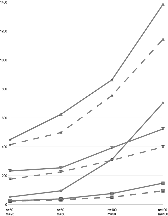
Remark 3

Although Andersen (1998 – 2010, p. 131, Section 7.2 and 7.2.1) recommends to rather use the MOSEK SOCP-solver than the MOSEK QCQP-solver for solving convex QCQPs, this does not coincide with the above results in which the MOSEK QCQP-solver has a significantly better performance than the MOSEK SOCP-solver for solving a QCQP of our shape.

The results from Figures 1–5 suggest that we will only test the MOSEK QCQP-solver on the reduced QCQP (10) in higher dimensions as this is the only combination that does not significantly exceed the shortest duration for solving the corresponding QP (which is always achieved by the MOSEK QP-solver). Therefore, we plot in Figure 6 (based on the data from Table 3 in appendix B of Fendl & Schichl ()) the minimal & maximal (lower and upper end of the vertical line) and the median (horizontal line) solving times (in milliseconds) obtained by MOSEK for L (black) and R (grey) (from $n=m=400$ on, our computer started to swap and, consequently, we did not test higher dimensional problems).

These results justify that we will mainly concentrate on the reduced QCQP (10) in the implementation as it is the only QCQP for which the solving time is competitive to that of the corresponding QP.

4 Numerical results

In the following section we compare the numerical results of our second order bundle algorithm with MPBNGC by Mäkelä (2003) and SolvOpt by Kappel & Kuntsevich (2000) for some examples of the Hock-Schittkowski collection by Schittkowski (2009a); Schittkowski (2009b), for custom examples that arise in the context of finding exclusion boxes for a quadratic CSP in GloptLab by Domes (2009), and for higher dimensional piecewise quadratic examples.

4.1 Introduction

There are three implementations of Algorithm 2.1 available: A pure MATLAB version (for easy understanding, modifying and testing new ideas concerning the algorithm); a MATLAB version in which the main parts of the algorithm are split into several subroutines, where every subroutine can either be called as pure MATLAB code or via a C mex-file (this is useful for partially speeding up the algorithm, but still keeping it simple enough for modifying and testing many examples of the modified code); and a pure C version (for performance), which is used throughout all the tests. The C mex-files and the C version require a BLAS/LAPACK implementation (e.g., ATLAS by Whaley & Petitet (2005), GotoBLAS by Goto & van de Geijn (2008), or the Netlib BLAS reference implementation by Blackford et al. (2002)). In the unconstrained case, all three versions produce the same results as the original FORTRAN bundle-Newton method by Lukšan & Vlček (1998).

Although there exist some test collections for nonsmooth unconstrained optimization (e.g., Lukšan & Vlček (2003)) and nonsmooth linearly constrained optimization (e.g., Lukšan & Vlček (2000); also cf. Karmitsa et al. (2009) for an extensive comparison of numerical results), we do not know a standardized, prominent test collection for nonsmooth constrained optimization. Therefore, a common way for testing nonsmooth constrained solvers is to take a test collection for smooth constrained optimization (e.g., the Hock-Schittkowski collection from Schittkowski (2009a); Schittkowski (2009b)) and to treat the smooth constraints as one nonsmooth constraint (by using a $\max$ -function).

We will make tests for

•

Algorithm 2.1 (with optimality tolerance $\varepsilon:=10^{-5}$ ), where we refer to the linearly constrained version as “BNLC”, to the version with the QCQP (9) as “Full Alg(orithm)”, and to the version with the reduced QCQP (10) as “Red(uced) Alg(orithm)”
•

MPBNGC by Mäkelä (2003) (with the standard termination criteria; although MPBNGC supports the handling of multiple nonsmooth constraints, we do not use this feature, since we are interested here, how well the different solvers handle the nonsmoothness of a constraint, i.e. without exploiting the knowledge of the structure of a $\max$ -function; since MPBNGC turned out to be very fast with respect to pure solving time for the low dimensional examples in the case of successful termination with a stationary point, the number of iterations and function evaluations was chosen in a way that in the other case the solving times of the different algorithms have approximately at least the same magnitude)
•

SolvOpt by Kappel & Kuntsevich (2000) (with the standard termination criteria, which are described in Kuntsevich & Kappel (1997))

(we choose MPBNGC and SolvOpt for our comparisons, since both are written in a compiled programming language, both are publicly available, and both support nonconvex constraints), where we will modify the termination criteria slightly only in Subsection 4.4, on the following examples (the corresponding result tables can be found in Fendl & Schichl ()):

•

Optimization problem (2) with $f(x):=\big(x_{1}+\tfrac{1}{2}\big)^{2}+\big(x_{2}+\tfrac{3}{2}\big)^{2}$ and $F(x):=\max\hat{F}_{1:2}(x)$ (denoted by E1) resp. $F(x):=\max(-\hat{F}_{1:2}(x),\hat{F}_{3}(x))$ (denoted by E2), where $\hat{F}_{1}(x):=x_{1}^{2}+x_{2}^{2}-1$ , $\hat{F}_{2}(x):=(x_{1}-1)^{2}+(x_{2}+1)^{2}-1$ , and $\hat{F}_{3}(x):=(x_{1}-1)^{2}-x_{2}-1$ , the example from Fendl & Schichl (2011, p. 10, Example 3.7) (denoted by E3) and the Hock-Schittkowski collection (in the above sense; no problems which contain nonlinear equality constraints; linear constraints are inserted into the search direction problem in Algorithm 2.1; feasible starting point). This yields 58 test problems which we will discuss in Subsection 4.2.
•

Optimization problems as described in Fendl et al. (2011, p. 9, Optimization problems (55) and (56)) (for finding exclusion boxes for CSPs; where the nonlinear part of these optimization problems is given by the certificate from Fendl et al. (2011, p. 5, Equation (35)), which we will discuss in Subsection 4.3.
•

Higher dimensional piecewise quadratic examples with up to 100 variables which we will discuss in Subsection 4.4.

All test examples will be sorted with respect to the problem dimension (beginning with the smallest). Furthermore, we use analytic derivative information for all occurring functions (Note: Implementing analytic derivative information for the certificate from Fendl et al. (2011, p. 5, Equation (35)) effectively, is a nontrivial task) and we perform all tests on the same machine as in Subsection 3.3.

We introduce the following notation for the record of the solution process of an algorithm (which is used in this section as well as in Fendl & Schichl ()).

Notation 4.1

We define

	N	$\displaystyle:=\textnormal{``Dimension of the optimization problem''}$
	Nit	$\displaystyle:=\textnormal{``Number of performed iterations''}\textnormal{\penalty\ ,}$

we denote the final number of evaluations of function dependent data by

	Na	$\displaystyle:=\textnormal{``Number of calls to }(f,g,G,F,\hat{g},\hat{G})\textnormal{'' (Algorithm \ref{BundleSQPmitQCQP:Alg:GesamtAlgMitQCQP})}$
	Nb	$\displaystyle:=\textnormal{``Number of calls to }(f,g,F,\hat{g})\textnormal{'' (MPBNGC)}$
	Nc	$\displaystyle:=\textnormal{``Number of calls to }(f,F)\textnormal{'' (SolvOpt)}$
	Ng	$\displaystyle:=\textnormal{``Number of calls to }g\textnormal{'' (SolvOpt)}$
	$\displaystyle\textnormal{N}\hat{\textnormal{g}}$	$\displaystyle:=\textnormal{``Number of calls to }\hat{g}\textnormal{'' (SolvOpt)}\textnormal{\penalty\ ,}$

we denote the duration of the solution process by

	$\textnormal{t}_{1}$	$\displaystyle:=\textnormal{``Time in milliseconds''}$
	$\textnormal{t}_{2}$	$\displaystyle:=\textnormal{``Time in milliseconds (without (QC)QP)'' (only relevant for Algorithm \ref{BundleSQPmitQCQP:Alg:GesamtAlgMitQCQP})}$

and we denote the additional algorithmic information by

	R	$\displaystyle:=\textnormal{``Remark'' (e.g., if }t_{0}^{k}\textnormal{ is modified in Algorithm \ref{BundleSQPmitQCQP:Alg:GesamtAlgMitQCQP},}$
		additional SolvOpt termination information,
		supplementary problem dependent facts,…)
	nt	$\displaystyle:=\textnormal{``No termination'' (within the given number of Nit,\ldots)}$
	wm	$\displaystyle:=\textnormal{``Wrong minimum''}\textnormal{\penalty\ .}$

Remark 4

In particular the percentage of the time spent in the (QC)QP in Algorithm 2.1 is given by

p_{1}:=\tfrac{\textnormal{$\textnormal{t}_{1}$}(\textnormal{Algorithm \ref{BundleSQPmitQCQP:Alg:GesamtAlgMitQCQP}})-\textnormal{$\textnormal{t}_{2}$}(\textnormal{Algorithm \ref{BundleSQPmitQCQP:Alg:GesamtAlgMitQCQP}})}{\textnormal{$\textnormal{t}_{1}$}(\textnormal{Algorithm \ref{BundleSQPmitQCQP:Alg:GesamtAlgMitQCQP}})}\textnormal{\penalty\ .}

(11)

For comparing the cost of evaluating function dependent data (like, e.g., function values, subgradients,…) in a preferably fair way (especially for solvers that use different function dependent data), we will make use of the following realistic “credit point system” that an optimal implementation of algorithmic differentiation in backward mode suggests (cf. Griewank & Corliss (1991) and Schichl (2004); Schichl (); Schichl (2003)).

Definition 1

Let $f_{A}$ , $g_{A}$ and $G_{A}$ resp. $F_{A}$ , $\hat{g}_{A}$ and $\hat{G}_{A}$ be the number of function values, subgradients and (substitutes of) Hessians of the objective function resp. the constraint that an algorithm $A$ used for solving a nonsmooth optimization problem which may have linear constraints and at most one single nonsmooth nonlinear constraint. Then we define the cost of these evaluations by

c(A):=f_{A}+3g_{A}+3N\cdot G_{A}+\textnormal{nlc}\cdot(F_{A}+3\hat{g}_{A}+3N\cdot\hat{G}_{A})\textnormal{\penalty\ ,}

(12)

where $\textnormal{nlc}=1$ if the optimization problem has a nonsmooth nonlinear constraint, and $\textnormal{nlc}=0$ otherwise.

Since Algorithm 2.1 evaluates $f$ , $g$ , $G$ and $F$ , $\hat{g}$ , $\hat{G}$ at every call that computes function dependent data, we obtain

c(\textnormal{Algorithm \ref{BundleSQPmitQCQP:Alg:GesamtAlgMitQCQP}})=(1+\textnormal{nlc})\cdot\textnormal{Na}\cdot(1+3+3N)\textnormal{\penalty\ .}

Since MPBNGC evaluates $f$ , $g$ and $F$ , $\hat{g}$ at every call that computes function dependent data (cf. Mäkelä (2003)), the only difference to Algorithm 2.1 with respect to $c$ from (12) is that MPBNGC uses no information of Hessians and hence we obtain

c(\textnormal{MPBNGC})=(1+\textnormal{nlc})\cdot\textnormal{Nb}\cdot(1+3)\textnormal{\penalty\ .}

Since SolvOpt evaluates $f$ and $F$ at every call that computes function dependent data and only sometimes $g$ or $\hat{g}$ (cf. Kuntsevich & Kappel (1997)), we obtain

c(\textnormal{SolvOpt})=(1+\textnormal{nlc})\cdot\textnormal{Nc}+3(\textnormal{Ng}+\textnormal{nlc}\cdot\textnormal{N}\hat{g})\textnormal{\penalty\ .}

We will visualize the performance of two algorithms $A$ and $B$ for $s\in\{c,\textnormal{Nit}\}$ in Subsection 4.2 and Subsection 4.3 by the following record-plot: In this plot the abscissa is labeled by the name of the test example and the value of the ordinate is given by $\textnormal{rp}(s):=s(B)-s(A)$ (i.e. if $\textnormal{rp}(s)>0$ , then $\textnormal{rp}(s)$ tells us how much better algorithm $A$ is than algorithm $B$ with respect to $s$ for the considered example in absolute numbers; if $\textnormal{rp}(s)<0$ , then $\textnormal{rp}(s)$ quantifies the advantage of algorithm $B$ in comparison to algorithm $A$ ; if $\textnormal{rp}(s)=0$ , then both algorithms are equally good with respect to $s$ ). The scaling of the plots is chosen in a way that plots that contain the same test examples are comparable (although the plots may have been generated by results from different algorithms).

Remark 5

All results for Algorithm 2.1 that are given in the tables of Fendl & Schichl ()) were obtained by using MOSEK by Andersen et al. (2003) for determining the search direction, where we used the MOSEK QCQP-solver which turned out to be much faster than the MOSEK SOCP-solver again (as we already noticed in Remark 3). We emphasize that in our tests there occurred no search direction problem which MOSEK was not able to solve.

The results for computing the search direction in Algorithm 2.1 with IPOPT by Wächter & Biegler (2006) are practically the same with respect to Nit and Na. Furthermore, IPOPT was as robust and reliable as MOSEK. Nevertheless, IPOPT was slower than MOSEK with respect to the solving time which we expected as IPOPT is designed for general non-linear optimization problems, while MOSEK is specialized in particular for QCQPs.

When using socp by Lobo et al. (1997) for the computation of the search direction in Algorithm 2.1, the results are also practically the same with respect to Nit and Na — as long as socp did not fail to solve the search direction problem: The most successful effort of stabilizing socp was achieved by the following idea from SEDUMI by Sturm (1998 – 2001); Pólik (2005): We added an additional termination criterion to socp as it is used in SEDUMI, if SEDUMI cannot achieve the desired accuracy for the duality gap (the additional termination criterion is referred to as pars.bigeps in SEDUMI): If the current duality gap is smaller than $\texttt{bigeps}:=10^{-2}$ and differs at most by $10^{-5}$ from the duality gap of the last iteration, then we accept the current point as a solution. In our empirical experiments socp tended to be more reliable, when we chose certatin SOCP-dependent parameters according to Fendl (2011, p. 123, Equation (4.57)). We were not able to make socp more robust by improving the strict feasibility of the starting point by solving various linear programs that are obtained from the primal SOCP and the dual SOCP by exploiting the fact that $\lvert x\rvert_{{}_{2}}\leq\lvert x\rvert_{{}_{1}}$ for all $x\in\mathbb{R}^{n}$ (lp_solve by Berkelaar et al. (2004), which is based on the revised simplex method and which we used for computing a solution of these linear programs, solved all of them easily).

At least when we used the variant of socp which was best for our purposes (i.e. socp with a bigeps-termination criterion) in Algorithm 2.1, then we were able to solve all examples that we took from the Hock-Schittkowski collection, while we were not able to achieve this for the other variants of socp. Furthermore, many examples of the nonlinearly constrained optimization problem from Fendl et al. (2011, p. 9, Optimization problems (55) and (56)) were not solvable by Algorithm 2.1 when using socp for the computation of the search direction (even when we used the best variant of socp).

4.2 Hock-Schittkowski Test-set

From Table 4 in Fendl & Schichl (), in which the results for the Hock-Schittkowski collection can be found and which is the basis for all plots in this subsection, we draw the following conclusions:

To compare the solving time $t_{1}$ for the reduced algorithm (with MOSEK as (QC)QP-solver) and MPBNGC, we consider

	$\textnormal{t}_{1}$ (Red Alg)	$\textnormal{t}_{2}$ (Red Alg)	$p_{1}$	$\textnormal{t}_{1}$ (MPBNGC)
HS	1198	961	0.80	1386
HS (*)	902	751	0.83	154

where we make use of (11) and in (*) we consider only those examples for which MPBNGC satisfied one of its termination criteria (cf. Subsubsection 4.3.5). Hence, for those examples of the Hock-Schittkowski collection for which MPBNGC was able to terminate successfully, MPBNGC is faster than the reduced algorithm. Furthermore, we notice that the reduced algorithm spent at least 80% of its time in the QCQP-solver, which is mostly overhead time in particular for the examples with lower dimension (which most examples are) as MOSEK has to, e.g., set up sparse matrix structures.

The reduced algorithm needs approximately 65% of the solving time $t_{1}$ of the full algorithm. Nevertheless, SolvOpt only needs approximately 23% resp. 36% of the solving time $t_{1}$ of the full algorithm resp. the reduced algorithm. Not surprisingly, the full algorithm spent 80% of the time for solving the QCQPs (like the reduced algorithm did). Since SolvOpt terminated for the higher dimensional examples (i.e. the 15-dimensional examples 284, 285 and 384) with points that are not stationary, while both the full and the reduced algorithm were able to solve them, and since the reduced algorithm needs significantly less pure solving time than the full algorithm for these examples

ex	$\textnormal{t}_{1}$ $($ Full Alg $)$	$\textnormal{t}_{1}$ $($ Red Alg $)$	$p_{2}$
284	92	46	0.50
285	796	140	0.18
384	589	125	0.21

where $p_{2}:=\tfrac{\textnormal{$\textnormal{t}_{1}$}(\textnormal{Red Alg})}{\textnormal{$\textnormal{t}_{1}$}(\textnormal{Full Alg})}$ , we may expect that for more difficult examples the performance of the reduced algorithm increases with respect to $t_{1}$ (cf. Subsubsection 4.3.2 and Subsection 4.4).

Therefore, we will concentrate our comparison of Algorithm 2.1 (full and reduced version), MPBNGC and SolvOpt on the qualitative aspects of the cost $c$ of the evaluations (solid line) and the number of iterations Nit (dashed line; this comparison is only meaningful for the comparison between the full algorithm and the reduced algorithm), where we use the two different line types for a better distinction of the comparisons in Figure 7, in this subsection, where before making detailed comparisons of our 58 examples, we give a short overview of them as a reason of clarity of the presentation: This yields the following summary table consisting of the number of examples for which the reduced algorithm is better than the full algorithm, MPBNGC resp. SolvOpt (and vice versa)

	no termi-	significantly	better	a bit	nearly	a bit	better	significantly
	nation	better		better	equal	better		better
(Color code: Light grey)	Full Alg					Red Alg
Nit	0	2	1	3	51	0	1	0
$c$	0	4	1	7	40	1	1	4
(Color code: Grey)	MPBNGC					Red Alg
$c$	5	2	3	10	16	8	7	7
(Color code: Black)	SolvOpt					Red Alg
$c$	3	3	4	3	1	31	9	4

that is visualized in Figure 7

Figure 7: Hock-Schittkowski collection (summary)

and that let us draw the following conclusions: The performances of the full algorithm and the reduced algorithm are quite similar. The reduced algorithm is superior to MPBNGC in one third of the examples, for a further third of the examples one of these two solvers has only small advantages over the other, the performance differences between the two algorithms considered can be completely neglected for one quarter of the examples, and for the remaining ten percent of the examples MPBNGC beats the reduced algorithm clearly. The reduced algorithm is superior to SolvOpt in about one quarter of the examples, for sixty percent of the examples one of these two solvers has only small advantages over the other (in most cases the reduced algorithm is the slightly more successful one), and in the remaining twelve percent of the examples SolvOpt beats the reduced algorithm clearly.

Furthermore, only the full algorithm and the reduced algorithm solved all examples successfully.

Reduced algorithm vs. Full algorithm

First of all, in the full algorithm $t_{0}^{k}$ is only modified in 11 examples (34, 43, 66, 83, 100, 113, 227, 230, 264, 285, 384), while in the reduced algorithm this happens in 14 examples (the additional examples are 284, 330, 341). In all these examples $t_{0}^{k}$ is only modified a few times and a modification only occurs at very early iterations of the optimization process (cf. Fendl & Schichl (2011, p. 19, Remark 3.16)).

From Figure 14 and Figure 15 in Fendl & Schichl () we conclude that the full and the reduced algorithm produce in most of the 58 examples approximately the same results — exceptions from this observation are in view of iterations the following 7 examples: The reduced algorithm is better in 1 example in comparison with the full algorithm, while the full algorithm is significantly better in 2 examples, better in 1 example and a bit better in 3 examples in comparison with the reduced algorithm.

In view of costs the exceptions are given by the following 18 examples: The reduced algorithm is significantly better in 4 examples, better in 1 example (33) a bit better in 1 example in comparison with the full algorithm, while the full algorithm is significantly better in 4 examples, better in 1 example and a bit better in 7 examples in comparison with the reduced algorithm.

Reduced algorithm vs. MPBNGC

MPBNGC does not satisfy any of its termination criteria for five examples (15, 20, 83, 285 and 384) within the given number of iterations and function evaluations. For the other 53 examples from Figure 16 in Fendl & Schichl () we emphasize the following ones: The reduced algorithm is significantly better in 7 examples, better in 7 examples and a bit better in 8 examples in comparison with MPBNGC, while MPBNGC is significantly better in 2 examples, better in 3 examples and a bit better in 10 examples in comparison with the reduced algorithm. In the remaining 16 examples the cost of the reduced algorithm and MPBNGC is practically the same.

Reduced algorithm vs. SolvOpt

SolvOpt terminates for the three 15-dimensional examples 284, 285 and 384 with points that are not stationary. For the other 55 examples from Figure 17 in Fendl & Schichl () we emphasize the following ones: The reduced algorithm is significantly better in 4 examples and better in 9 examples in comparison with SolvOpt, while SolvOpt is significantly better in 3 examples, better in 4 examples and a bit better in 3 examples in comparison with the reduced algorithm. Except for example 233 in which the cost of the reduced algorithm and SolvOpt are practically the same, in all 31 remaining examples the reduced algorithm is a bit better than SolvOpt.

4.3 Exclusion boxes

4.3.1 Basics

We consider the quadratic CSP

\begin{split}F(x)&\in\boldsymbol{F}\\ x&\in\boldsymbol{x}\end{split}

(13)

and we assume that a solver, which is able to solve a CSP, takes the box $\boldsymbol{u}:=[\underline{u},\overline{u}]\subseteq\boldsymbol{x}$ into consideration during the solution process. Fendl et al. (2011, ) constructed a certificate of infeasibility $f$ , which is a nondifferentiable and nonconvex function in general, with the following property: If there exists a vector $y$ with

f(y,\underline{u},\overline{u})<0\textnormal{\penalty\ ,}

(14)

then the CSP (13) has no feasible point in $\boldsymbol{u}$ and consequently this box can be excluded for the rest of the solution process. Therefore, a box $\boldsymbol{u}$ for which (14) holds is called an exclusion box.

The obvious way for finding an exclusion box for the CSP (13) is to minimize $f$

\begin{split}\min_{y}{f(y,\underline{u},\overline{u})}\end{split}

and stop the minimization if a negative function value occurs. We will give results for this linearly constrained optimization problem with a fixed box (i.e. without optimizing $u$ and $v$ ) for dimensions between $4$ and $11$ in Subsubsection 4.3.3.

To find at least an exclusion box $\boldsymbol{v}:=[\underline{v},\overline{v}]\subseteq\boldsymbol{u}$ with $\underline{v}+r\leq\overline{v}$ , where $r\in(0,\overline{u}-\underline{u})$ is fixed, we can try to solve

\begin{split}&\min_{y,\underline{v},\overline{v}}{f(y,\underline{v},\overline{v})}\\ &\textnormal{ s.t. }[\underline{v}+r,\overline{v}]\subseteq\boldsymbol{u}\textnormal{\penalty\ ,}\end{split}

where the results for this linearly constrained optimization problem with a variable box (i.e. with optimizing $u$ and $v$ ) for dimensions between $8$ and $21$ are discussed in Subsubsection 4.3.4.

Moreover, we can enlarge an exclusion box $\boldsymbol{v}$ by solving

\begin{split}&\max_{y,\underline{v},\overline{v}}{\mu(\underline{v},\overline{v})}\\ &\textnormal{ s.t. }f(y,\underline{v},\overline{v})\leq\delta\textnormal{\penalty\ ,}\penalty\ [\underline{v},\overline{v}]\subseteq\boldsymbol{u}\textnormal{\penalty\ ,}\end{split}

where $\delta<0$ is given and $\mu(\underline{v},\overline{v}):=\lvert\left(\begin{smallmatrix}\underline{v}-\underline{x}\\ \overline{v}-\overline{x}\end{smallmatrix}\right)\rvert_{{}_{1}}$ measures the magnitude of the box $\boldsymbol{v}$ , and we regard an exclusion box as sufficiently large, if the objective function satisfies $\mu(\underline{v},\overline{v})\leq 10^{-6}$ . The discussion of the results of this nonlinearly constrained optimization problem for dimension $8$ can be found in in Subsubsection 4.3.5.

The underlying data for these nonsmooth optimization problems was extracted from real CSPs that occur in GloptLab by Domes (2009). Apart from $u$ and $v$ , we will concentrate on the optimization of the variables $y$ and $z$ due to the large number of tested examples (cf. Subsubsection 4.3.2), and since the additional optimization of $R$ and $S$ did not have much impact on the quality of the results which was discovered in additional empirical observations, where a detailed analysis of these observations goes beyond the scope of this paper. Furthermore, we will make our tests for the two different choices $T=1$ and $T=\lvert y\rvert_{{}_{2}}$ of the function $T$ , which occurs in the denominator of the certificate $f$ from Fendl et al. (2011, p. 5, Equation (35)), where for the latter one $f$ is only defined outside of the zero set of $T$ which has measure zero — although the convergence theory of many solvers (cf., e.g., Fendl & Schichl (2011, p. 7, 3.1 Theoretical basics)) requires that all occurring functions are defined on the whole space.

Remark 6

Because SolvOpt cannot distinguish between linear and nonlinear constraints (cf. Kuntsevich & Kappel (1997, p. 15)), the linear constraints of the linearly constrained optimization problems from Fendl et al. (2011, p. 9, Optimization problem (55) and (56)) must be formulated as nonlinear constraints in SolvOpt. Nevertheless, we will not include the number of these evaluations in the computation of the cost $c$ from (12) for the mentioned optimization problems in Subsubsection 4.3.3 and Subsubsection 4.3.4, since these evaluations may be considered as easy in comparison to the evaluation of the certificate $f$ from Fendl et al. (2011, p. 5, Equation (35)) which is the objective function in these optimization problems.

4.3.2 Overview of the results

We compare the total time $t_{1}$ of the solution process, where we used the reduced algorithm (with MOSEK as the (QC)QP-solver) in the constrained case: From Tables 5–8 (s. Fendl & Schichl ()) we obtain

	$\textnormal{t}_{1}$ (Red Alg)	$\textnormal{t}_{2}$ (Red Alg)	$p_{1}$	$\textnormal{t}_{1}$ (MPBNGC)	$\textnormal{t}_{1}$ (SolvOpt)
	$T=1$
Linearly constrained (fixed box)	1477	215	0.85	231	2754
Linearly constrained (variable box)	782	60	0.92	30	1546
Nonlinearly constrained	25420	4885	0.81	21860	38761
Nonlinearly constrained (*)	19053	3723	0.80	2067	30312
	$T=\lvert y\rvert_{{}_{2}}$
Linearly constrained (fixed box)	1316	129	0.90	15	1508
Linearly constrained (variable box)	797	45	0.94	30	2263
Nonlinearly constrained	24055	4284	0.82	25383	16909
Nonlinearly constrained (*)	18038	3112	0.83	3719	12635

where we make use of (11) and in (*) we consider only those examples for which MPBNGC satisfied one of its termination criteria (cf. Subsubsection 4.3.5).

For the linearly constrained problems MPBNGC was the fastest of the tested algorithms, followed by BNLC and SolvOpt. If we consider only those nonlinearly constrained examples for which MPBNGC was able to terminate successfully, MPBNGC was the fastest algorithm again. Considering the competitors, for the nonlinearly constrained problems with $T=1$ the reduced algorithm is 13.3 seconds resp. 11.3 seconds faster than SolvOpt, while for the nonlinearly constrained problems with $T=\lvert y\rvert_{{}_{2}}$ SolvOpt is 7.1 seconds resp. 5.4 seconds faster than the reduced algorithm.

Again (cf. Subsection 4.2), taking a closer look at $p_{1}$ yields the observation that at least 85% of the time is consumed by solving the QP (in the linearly constrained case) resp. at least 80% of the time is consumed by solving the QCQP (in the nonlinearly constrained case), which implies that the difference in the percentage between the QP and the QCQP is small in particular (an investigation of the behavior of the solving time $t_{1}$ for higher dimensional problems can be found in Subsection 4.4).

Therefore, we will concentrate in Subsubsection 4.3.3, Subsubsection 4.3.4 and Subsubsection 4.3.5 on the comparison of qualitative aspects between Algorithm 2.1, MPBNGC and SolvOpt (like, e.g., the cost $c$ of the evaluations), where before making these detailed comparisons, we give a short overview of them as a reason of clarity of the presentation: In both cases $T=1$ (solid line) and $T=\lvert y\rvert_{{}_{2}}$ (dashed line), where we use the two different line types for a better distinction in the following, we tested 128 linearly constrained examples with a fixed box, 117 linearly constrained examples with a variable box and 201 nonlinearly constrained examples, which yields the following two summary tables consisting of the number of examples for which Algorithm 2.1 (BNLC resp. the reduced algorithm) is better than MPBNGC resp. SolvOpt (and vice versa) with respect to the cost $c$ of the evaluations

(Color code: Light grey)	MPBNGC					BNLC/Red Alg
	no termi-	significantly	better	a bit	nearly	a bit	better	significantly
	nation	better		better	equal	better		better
					$T=1$
Linearly constrained (fixed box)	0	2	5	12	106	2	0	1
Linearly constrained (variable box)	0	0	0	1	116	0	0	0
Nonlinearly constrained	32	6	28	89	31	10	2	3
					$T=\lvert y\rvert_{{}_{2}}$
Linearly constrained (fixed box)	0	2	5	30	91	0	0	0
Linearly constrained (variable box)	0	0	0	5	112	0	0	0
Nonlinearly constrained	43	4	28	59	30	15	14	8

(Color code: Black)	SolvOpt					BNLC/Red Alg
	no termi-	significantly	better	a bit	nearly	a bit	better	significantly
	nation	better		better	equal	better		better
					$T=1$
Linearly constrained (fixed box)	0	1	3	0	61	25	13	25
Linearly constrained (variable box)	0	0	0	0	48	37	24	8
Nonlinearly constrained	0	0	14	20	21	76	20	50
					$T=\lvert y\rvert_{{}_{2}}$
Linearly constrained (fixed box)	0	1	2	1	32	34	49	9
Linearly constrained (variable box)	0	0	0	5	41	32	19	20
Nonlinearly constrained	0	2	24	26	31	61	45	12

that are visualized in Figures 8, 9, and 10

Figure 8: Linearly constrained — fixed box (summary)

Figure 9: Linearly constrained — variable box (summary)

Figure 10: Nonlinearly constrained (summary)

and that let us draw the following conclusions:

The performance differences between BNLC and MPBNGC can be neglected for the largest part of the linearly constrained examples (with small advantages for MPBNGC in about ten percent of these examples). For the nonlinearly constrained examples the reduced algorithm is superior to MPBNGC in one quarter of the examples, for forty percent of the examples one of these two solvers has small advantages over the other (in most cases MPBNGC is the slightly more successful one), the performance differences between the two algorithms considered can be completely neglected for fifteen percent of the examples, and for further fifteen percent of the examples MPBNGC beats the reduced algorithm clearly.

For the linearly constrained examples BNLC is superior to SolvOpt in one third of the examples, for one quarter of the examples one of these two solvers has small advantages over the other (in nearly all cases BNLC is the slightly more successful one), the performance differences between the two algorithms considered can be completely neglected for forty percent of the examples, and in only one percent of the examples SolvOpt beats the reduced algorithm clearly. For the nonlinearly constrained examples the reduced algorithm is superior to SolvOpt in one third of the examples, for 45 percent of the examples one of these two solvers has small advantages over the other (the reduced algorithm is often the slightly more successful one), the performance differences between the considered two algorithms can be completely neglected for ten percent of the examples, and in the remaining ten percent of the examples SolvOpt beats the reduced algorithm clearly.

In contrast to the linearly constrained case, in which all three solvers terminated successfully for all examples, only the reduced algorithm and SolvOpt were able to attain this goal in the nonlinearly constrained case, too.

4.3.3 Linearly constrained case (fixed box)

We took 310 examples from real CSPs that occur in GloptLab. We observe that for 79 examples the starting point is feasible for the CSP and for 103 examples the evaluation of the certificate at the starting point identifies the box as infeasible and hence there remain 128 test problems.

BNLC vs. MPBNGC

In the case $T=1$ we conclude from Figure 18 in Fendl & Schichl () that BNLC is significantly better in 1 example and a bit better in 2 examples in comparison with MPBNGC, while MPBNGC is significantly better in 2 examples, better in 5 examples and a bit better in 12 examples in comparison with BNLC. In the 106 remaining examples the costs of BNLC and MPBNGC are practically the same.

In the case $T=\lvert y\rvert_{{}_{2}}$ it follows from Figure 19 in Fendl & Schichl () that MPBNGC is significantly better in 2 examples, better in 5 examples and a bit better in 30 examples in comparison with BNLC. In the 91 remaining examples the costs of BNLC and MPBNGC are practically the same.

BNLC vs. SolvOpt

In the case $T=1$ we conclude from Figure 20 in Fendl & Schichl () that BNLC is significantly better in 25 examples, better in 13 examples and a bit better in 25 examples in comparison with SolvOpt, while SolvOpt is significantly better in 1 example and better in 3 examples in comparison with BNLC. In the 61 remaining examples the costs of BNLC and SolvOpt are practically the same.

In the case $T=\lvert y\rvert_{{}_{2}}$ it follows from Figure 21 in Fendl & Schichl () that BNLC is significantly better in 9 examples, better in 49 examples and a bit better in 34 examples in comparison with SolvOpt, while SolvOpt is significantly better in 1 example, better in 2 examples and a bit better in 1 example in comparison with BNLC. In the 32 remaining examples the costs of BNLC and SolvOpt are practically the same.

4.3.4 Linearly constrained case (variable box)

We observe that for 80 examples the starting point is feasible for the CSP and for 113 examples the evaluation of the certificate at the starting point identifies the boxes as infeasible and hence there remain 117 test problems of the 310 original examples from GloptLab.

BNLC vs. MPBNGC

In the case $T=1$ we conclude from Figure 22 in Fendl & Schichl () that MPBNGC is a bit better in 1 example in comparison with BNLC. In the 116 remaining examples the costs of BNLC and MPBNGC are practically the same.

In the case $T=\lvert y\rvert_{{}_{2}}$ it follows from Figure 23 in Fendl & Schichl () that MPBNGC is a bit better in 5 examples in comparison with BNLC. In the 112 remaining examples the costs of BNLC and MPBNGC are practically the same.

BNLC vs. SolvOpt

In the case $T=1$ we conclude from Figure 24 in Fendl & Schichl () that BNLC is significantly better in 8 examples, better in 24 examples and a bit better in 37 examples in comparison with SolvOpt. In the 48 remaining examples the costs of BNLC and SolvOpt are practically the same.

In the case $T=\lvert y\rvert_{{}_{2}}$ it follows from Figure 25 in Fendl & Schichl () that BNLC is significantly better in 20 examples, better in 19 examples and a bit better in 32 examples in comparison with SolvOpt, while SolvOpt is a bit better in 5 examples in comparison with BNLC. In the 41 remaining examples the costs of BNLC and SolvOpt are practically the same.

4.3.5 Nonlinearly constrained case

Since we were not able to find a starting point, i.e. an infeasible sub-box, for 109 examples, we exclude them from the following tests for which there remain 201 examples of the 310 original examples from GloptLab.

Reduced algorithm vs. MPBNGC

In the case $T=1$ MPBNGC does not satisfy any of its termination criteria for 32 examples within the given number of iterations and function evaluations (also cf. Subsubsection 4.3.1). For the remaining 169 examples we conclude from Figure 26 in Fendl & Schichl () that the reduced algorithm is significantly better in 3 examples, better in 2 examples and a bit better in 10 examples in comparison with MPBNGC, while MPBNGC is significantly better in 6 examples, better in 28 examples and a bit better in 89 examples in comparison with the reduced algorithm, and in 31 examples the costs of the reduced algorithm and MPBNGC are practically the same.

In the case $T=\lvert y\rvert_{{}_{2}}$ MPBNGC does not satisfy any of its termination criteria for 43 examples within the given number of iterations and function evaluations. For the remaining 158 examples it follows from Figure 27 in Fendl & Schichl () that the reduced algorithm is significantly better in 8 examples, better in 14 examples and a bit better in 15 examples in comparison with MPBNGC, while MPBNGC is significantly better in 4 examples, better in 28 examples and a bit better in 59 examples in comparison with the reduced algorithm, and in 30 examples the costs of the reduced algorithm and MPBNGC are practically the same.

Reduced algorithm vs. SolvOpt

In the case $T=1$ we conclude from Figure 28 in Fendl & Schichl () that the reduced algorithm is significantly better in 50 examples, better in 20 examples and a bit better in 76 examples in comparison with SolvOpt, while SolvOpt is better in 14 examples and a bit better in 20 examples in comparison with the reduced algorithm. In the 21 remaining examples the costs of the reduced algorithm and SolvOpt are practically the same.

In the case $T=\lvert y\rvert_{{}_{2}}$ it follows from Figure 29 in Fendl & Schichl () that the reduced algorithm is significantly better in 12 examples, better in 45 examples and a bit better in 61 examples in comparison with SolvOpt, while SolvOpt is significantly better in 2 examples, better in 24 examples and a bit better in 26 examples in comparison with the reduced algorithm. In the 31 remaining examples the costs of the reduced algorithm and SolvOpt are practically the same.

4.4 Higher dimensional piecewise quadratic examples

We want to give numerical results for the nonsmooth optimization problem (2) with

f(x):=\max_{i=1,\dots,m_{1}}{f_{i}(x)}\textnormal{\penalty\ ,}\quad F(x):=\max_{j=1,\dots,m_{2}}{F_{j}(x)}\textnormal{\penalty\ ,}

where

	$\displaystyle f_{i}(x)$	$\displaystyle:=\alpha_{i}+a_{i}^{T}(x-x_{i})+\tfrac{1}{2}(x-x_{i})^{T}A_{i}(x-x_{i})$
	$\displaystyle F_{j}(x)$	$\displaystyle:=\beta_{j}+b_{j}^{T}(x-x_{j})+\tfrac{1}{2}(x-x_{j})^{T}B_{j}(x-x_{j})$

and $\alpha_{i},\beta_{j}\in\mathbb{R}$ , $a_{i},b_{j}\in\mathbb{R}^{N}$ , $A_{i},B_{j}\in\mathbb{R}_{\mathrm{sym}}^{N\times N}$ , $x_{i},x_{j}\in\mathbb{R}^{N}$ .

The underlying data of the test examples was produced by a random number generator with the following restrictions concerning the data corresponding to $F$ : At least one $B_{j}$ is chosen as a positive definite matrix to guarantee that the feasible set is bounded, and after choosing $b_{j}$ , $B_{j}$ , $x_{j}$ as well as a starting point $x^{0}\in\mathbb{R}^{N}$ , $\beta_{j}$ is chosen such that $x^{0}$ is strictly feasible.

We made comparison tests for the dimensions $N\in\{20,40,60,80,100\}$ to investigate the behavior of the reduced algorithm ( $\square$ ), MPBNGC ( $\diamondsuit$ ) and SolvOpt ( $\nabla$ ), where we use the colors to distinguish the results of the different solvers, with respect to the solving time $t_{1}$ and successful termination, and we focus on the larger values of $N$ (due to the magnitude of $N$ , we did not test the full version of Algorithm 2.1). Moreover, we chose $m_{1}:=\tfrac{N}{10}$ and $m_{2}\in\{\tfrac{N}{2},N\}$ , so that the emphasis of the examples lies on the handling of the constraint.

Furthermore, due to the magnitude of the test examples, we weakened the optimality tolerance of the reduced algorithm to $\varepsilon:=10^{-3}$ . Since the reduced algorithm terminated for all examples of this class of test functions with satisfying its termination criterion (which guarantees the stationarity of the computed point due to Fendl & Schichl (2011, )), we denote the minimizer (of the corresponding example) that was computed by the reduced algorithm by $\hat{x}$ .

Before the actual tests, we performed a few runs of the whole test set, where we started with very weak termination criteria for MPBNGC and SolvOpt and then sharpened them, with the goal to make the results between the different solvers comparable in the following way: If the computed minimizer is close to $\hat{x}$ , then approximately the same $F_{j}$ should be active. Based on these empirical observations, we made the final choices for the termination criteria of MPBNGC and SolvOpt, where we were quite successful to achieve this goal for MPBNGC, while we were not able to achieve it for SolvOpt in many cases (although putting a lot of effort into it).

For every pair $(N,m_{2})$ we tested $20$ different examples for two levels of difficulty that is classified by the average number of $j\in\{1,\dots,m_{2}\}$ with $\lvert F_{j}(\hat{x})-F(\hat{x})\rvert\leq 10^{-3}$ , which yields the following overview of our overall 400 different examples

Level	$m_{2}$	$N$
		20	40	60	80	100
Easy	$\tfrac{N}{2}$	4	4	6	6	7
	$N$	5	6	8	9	10
Difficult	$\tfrac{N}{2}$	4	8	12	15	19
	$N$	7	14	19	26	31

i.e. for given $N$ and $m_{2}$ we regard an example as more difficult, the more impact the constraint has at $\hat{x}$ (in the case of the successful termination of one of the solvers, there was always at least one $F_{j}$ active). Moreover, for a given level of difficulty, $N$ , and $m_{2}$ , the corresponding examples are sorted by the numbers $N-20+1,\dots,N$ .

Before making detailed comparisons of the obtained results (s. Tables 9–12 in Fendl & Schichl ()) in Subsubsections 4.4.1–4.4.4, we give a short overview of them as a reason of clarity of the presentation: For all $N\in\{20,40,60,80,100\}$ we summarize the easy examples and the difficult examples, where we use two different line types for a better distinction of the comparisons of $m_{2}$ (for $m_{2}=\tfrac{N}{2}$ we use a dashed line and for $m_{2}=N$ we use a solid line) in Figures 11 and 12, which yields the following two summary tables consisting of the number of examples for which the reduced algorithm is better than MPBNGC resp. SolvOpt (and vice versa) with respect to the solving time $\textnormal{t}_{1}$

(Color code: Grey)		MPBNGC					Red Alg
		no termi-	significantly	better	a bit	nearly	a bit	better	significantly
Level	$m_{2}$	nation	better		better	equal	better		better
Easy	$\tfrac{N}{2}$	1	18	17	18	27	6	5	8
	$N$	2	8	26	26	20	8	5	5
Difficult	$\tfrac{N}{2}$	73	0	4	5	4	3	2	9
	$N$	78	0	1	1	5	1	4	10

(Color code: Black)		SolvOpt					Red Alg
		no termi-	significantly	better	a bit	nearly	a bit	better	significantly
Level	$m_{2}$	nation	better		better	equal	better		better
Easy	$\tfrac{N}{2}$	18	14	25	11	15	6	7	4
	$N$	11	16	21	11	15	10	11	5
Difficult	$\tfrac{N}{2}$	3	4	16	3	8	15	28	23
	$N$	0	5	8	11	15	7	34	20

that are visualized in Figure 11 and Figure 12

Figure 11: Easy examples (summary)

Figure 12: Difficult examples (summary)

and that let us together with Figure 13, in which the solving times $t_{1}$ for all examples are plotted

Figure 13: Solving time

\textnormal{t}_{1}

for all higher dimensional piecewise quadratic examples

draw the following conclusions:

For the easy examples the reduced algorithm is superior to MPBNGC in thirteen percent of the examples, for thirty percent of the examples one of these two solvers has small advantages over the other (in most cases MPBNGC is the slightly more successful one), the performance differences between the considered two algorithms can be completely neglected for one quarter of the examples, and for one third of the examples MPBNGC beats the reduced algorithm clearly. MPBNGC was not able to terminate successfully for many of the difficult examples in particular for $N\in\{60,80,100\}$ despite significantly longer running times as it can be seen in Figure 13 (in additional test runs with a softer termination criterion MPBNGC did terminate for approximately half of the difficult examples, but the quality of the obtained minimizers was not comparable with the corresponding $\hat{x}$ produced by the reduced algorithm, while for the comparisons presented here this quality is comparable) and therefore the reduced algorithm is superior to MPBNGC in 88 percent of these examples. Furthermore, for five percent of the examples one of these two solvers has small advantages over the other, the performance differences between the considered two algorithms can be completely neglected for further five percent of the examples, and for the remaining two percent of the examples MPBNGC beats the reduced algorithm clearly.

For the easy examples the reduced algorithm is superior to SolvOpt in thirty percent of the examples, for fifteen percent of the examples one of these two solvers has small advantages over the other, the performance differences between the considered two algorithms can be completely neglected for further fifteen percent of the examples, and in the remaining forty percent of the examples SolvOpt beats the reduced algorithm clearly. For the difficult examples the reduced algorithm is superior to SolvOpt in a bit more than half of the examples (including many examples with $N\in\{80,100\}$ ), for twenty percent of the examples one of these two solvers has small advantages over the other, the performance differences between the considered two algorithms can be completely neglected for ten percent of the examples, and in the remaining (a bit less than) twenty percent of the examples SolvOpt beats the reduced algorithm clearly. In particular note that only very few $F_{j}$ are active at the points which SolvOpt found at termination for the easy examples (in comparison to both the reduced algorithm and MPBNGC), which might indicate that SolvOpt has some problems coming very close to the boundary. Although this behavior improves for the difficult examples, there still remains a clear gap in the number of active $F_{j}$ between SolvOpt and the other two solvers.

We want to emphasize the reduced algorithm was the only solver that terminated for all higher dimensional examples successfully, i.e. with a stationary point that is sufficiently accurate. Moreover, the solving times of the reduced algorithm are quite stable over all dimensions $N\in\{20,40,60,80,100\}$ .

Remark 7

Since MOSEK supports multiple CPUs in particular for solving QCQPs (cf. Andersen (1998 – 2010, p.152, 8.1.4 Using multiple CPU’s)), we may expect faster solving times for the reduced algorithm on such a system in particular for higher dimensional problems. Nevertheless, we have not been able to test this yet.

We also expect a significant improvement of the full algorithm if a QCQP-solver is used which exploits the special structure of the QCQP (4).

4.4.1 Easy examples with N/2 constraint components

We summarize the investigations of the results of the easy examples with $m_{2}:=\tfrac{N}{2}$ , which can be found in Table 9 in Fendl & Schichl () and which are visualized in Figure 30 in Fendl & Schichl ().

Reduced algorithm vs. MPBNGC

MPBNGC does not satisfy its termination criterion for one example within the given number of iterations and function evaluations. For the remaining 99 examples we obtain that the reduced algorithm is significantly better in 8 examples, better in 5 examples and a bit better in 6 examples in comparison with MPBNGC, while MPBNGC is significantly better in 18 examples, better in 17 examples a bit better in 18 examples in comparison with the reduced algorithm, and in 27 examples the solving times of both algorithms do not differ significantly.

Reduced algorithm vs. SolvOpt

SolvOpt does not satisfy its termination criterion for 18 examples within the given number of iterations and function evaluations. For the remaining 82 examples we obtain that the reduced algorithm is significantly better in 4 examples, better in 7 examples and a bit better in 6 examples in comparison with SolvOpt, while SolvOpt is significantly better in 14 examples, better in 25 examples and a bit better in 11 examples in comparison with the reduced algorithm, and in 15 examples the solving times of both algorithms do not differ significantly.

4.4.2 Easy examples with N constraint components

We summarize the investigations of the results of the easy examples with $m_{2}:=N$ , which can be found in Table 10 in Fendl & Schichl () and which are visualized in Figure 31 in Fendl & Schichl ().

Reduced algorithm vs. MPBNGC

MPBNGC does not satisfy its termination criterion for two examples within the given number of iterations and function evaluations. For the remaining 98 examples we obtain that the reduced algorithm is significantly better in 5 examples, better in 5 examples and a bit better in 8 examples in comparison with MPBNGC, while MPBNGC is significantly better in 8 examples, better in 26 examples and a bit better in 26 examples in comparison with the reduced algorithm, and in 20 examples the solving times of both algorithms do not differ significantly.

Reduced algorithm vs. SolvOpt

SolvOpt does not satisfy its termination criterion for 11 examples within the given number of iterations and function evaluations. For the remaining 89 examples we obtain that the reduced algorithm is significantly better in 5 examples, better in 11 examples and a bit better in 10 examples in comparison with SolvOpt, while SolvOpt is significantly better in 16 examples, better in 21 examples and a bit better in 11 examples in comparison with the reduced algorithm, and in 15 examples the solving times of both algorithms do not differ significantly.

4.4.3 Difficult examples with N/2 constraint components

We summarize the investigations of the results of the difficult examples with $m_{2}:=\tfrac{N}{2}$ , which can be found in Table 11 in Fendl & Schichl () and which are visualized in Figure 32 in Fendl & Schichl ().

Reduced algorithm vs. MPBNGC

MPBNGC does not satisfy its termination criterion for 73 examples within the given number of iterations and function evaluations. For the remaining 27 examples we obtain that the reduced algorithm is significantly better in 9 examples, better in 2 examples and a bit better in 3 examples in comparison with MPBNGC, while MPBNGC is better in 4 examples and a bit better in 5 examples in comparison with the reduced algorithm, and in 4 examples the solving times of both algorithms do not differ significantly.

Reduced algorithm vs. SolvOpt

SolvOpt does not satisfy its termination criterion for 3 examples within the given number of iterations and function evaluations. For the remaining 97 examples we obtain that the reduced algorithm is significantly better in 23 examples, better in 28 examples and a bit better in 15 examples in comparison with SolvOpt, while SolvOpt is significantly better in 4 examples, better in 16 examples and a bit better in 3 examples in comparison with the reduced algorithm, and in 8 examples the solving times of both algorithms do not differ significantly.

4.4.4 Difficult examples with N constraint components

We summarize the investigations of the results of the difficult examples with $m_{2}:=N$ , which can be found in Table 12 in Fendl & Schichl () and which are visualized in Figure 33 in Fendl & Schichl ().

Reduced algorithm vs. MPBNGC

MPBNGC does not satisfy its termination criterion for 78 examples within the given number of iterations and function evaluations. For the remaining 22 examples we obtain that the reduced algorithm is significantly better in 10 examples, better in 4 examples and a bit better in 1 example in comparison with MPBNGC, while MPBNGC is better in 1 example and a bit better in 1 example in comparison with the reduced algorithm, and in 5 examples the solving times of both algorithms do not differ significantly.

Reduced algorithm vs. SolvOpt

For our 100 examples we obtain that the reduced algorithm is significantly better in 20 examples, better in 34 examples and a bit better in 7 examples in comparison with SolvOpt, while SolvOpt is significantly better in 5 examples, better in 8 examples and a bit better in 11 examples in comparison with the reduced algorithm, and in 15 examples the solving times of both algorithms do not differ significantly.

5 Conclusion

In this paper we investigated numerical aspects of the feasible second order bundle algorithm for nonsmooth, nonconvex optimization problems with inequality constraints. Since one of the main characteristics of this method is that the search direction is determined by solving a convex QCQP, we investigated certain versions of the search direction problem and we justified the version chosen by us numerically by comparing the results of different solvers for the computation of the search direction. Furthermore, we made comparisons between the test results of our implementation of the second order bundle algorithm, MPBNGC by Mäkelä (2003) and SolvOpt by Kappel & Kuntsevich (2000) for some examples of the Hock-Schittkowski collection by Schittkowski (2009a); Schittkowski (2009b) and for custom examples that arise in the context of finding exclusion boxes for quadratic CSPs, where for both of these types of examples we were able to achieve good results with respect to the number of evaluations of function dependent data, as well as for higher dimensional piecewise quadratic examples, in which our implementation achieved good results in comparison with the other solvers in particular in the case that many constraint components were active at the solution. Summarizing the results it can be seen that the the SQP-like algorithm tends to compare the better the higher the dimension of the problem and the more difficult the nonsmoothness around the optimal point are.

References

Andersen (1998 – 2010) E.D. Andersen. The MOSEK C API manual. MOSEK ApS, Denmark, 1998 – 2010. Version 6.0 (Revision 66). URL http://www.mosek.com/.
Andersen et al. (2003) E.D. Andersen, C. Roos, and T. Terlaky. On implementing a primal-dual interior-point method for conic quadratic optimization. Mathematical Programming, B(95):249–277, 2003.
Berkelaar et al. (2004) M. Berkelaar, K. Eikland, and P. Notebaert. lp_solve. Open source (Mixed-Integer) Linear Programming system (Version 5.1.0.0), May 2004. URL http://lpsolve.sourceforge.net/.
Blackford et al. (2002) L.S. Blackford, J. Demmel, J. Dongarra, I. Duff, S. Hammarling, G. Henry, M. Heroux, L. Kaufman, A. Lumsdaine, A. Petitet, R. Pozo, K. Remington, and R.C. Whaley. An updated set of basic linear algebra subprograms (BLAS). ACM Transactions on Mathematical Software, 28(2):135–151, 2002. URL http://www.netlib.org/.
Burke et al. (2005) J.V. Burke, A.S. Lewis, and M.L. Overton. A robust gradient sampling algorithm for nonsmooth, nonconvex optimization. SIAM Journal on Optimization, 15(3):751–779, 2005.
Domes (2009) F. Domes. GloptLab – a configurable framework for the rigorous global solution of quadratic constraint satisfaction problems. Optimization Methods and Software, 24(4–5):727–747, 2009. URL http://www.mat.univie.ac.at/~dferi/gloptlab.html.
Fendl (2011) H. Fendl. A feasible second order bundle algorithm for nonsmooth, nonconvex optimization problems with inequality constraints and its application to certificates of infeasibility. PhD thesis, Universität Wien, 2011.
Fendl et al. (2011) H. Fendl, A. Neumaier, and H. Schichl. Certificates of infeasibility via nonsmooth optimization. In preparation, 2011.
(9) H. Fendl and H. Schichl. WWW-Document. URL http://www.mat.univie.ac.at/~herman/papers/FiguresAndResultTables.pdf.
Fendl & Schichl (2011) H. Fendl and H. Schichl. A feasible second order bundle algorithm for nonsmooth, nonconvex optimization problems with inequality constraints. In preparation, 2011.
Goto & van de Geijn (2008) K. Goto and R.A. van de Geijn. Anatomy of high-performance matrix multiplication. ACM Transactions on Mathematical Software, 34(3):12:1–12:25, 2008. URL http://www.tacc.utexas.edu/tacc-projects/gotoblas2/.
Grant & Boyd (2009) M. Grant and S. Boyd. CVX Users’ Guide for CVX version 1.2 (build 711), June 2009. URL http://cvxr.com/cvx/.
Griewank & Corliss (1991) A. Griewank and G.F. Corliss, editors. Automatic Differentiation of Algorithms: Theory, Implementation, and Application. SIAM, Philadelphia, PA, 1991.
Kappel & Kuntsevich (2000) F. Kappel and A.V. Kuntsevich. An implementation of Shor’s r-algorithm. Computational Optimization and Applications, 15(2):193–205, 2000.
Karmitsa et al. (2009) N. Karmitsa, A.M. Bagirov, and M.M. Mäkelä. Empirical and Theoretical Comparisons of Several Nonsmooth Minimization Methods and Software. TUCS Technical Report 959, Turku Centre for Computer Science, October 2009.
Kuntsevich & Kappel (1997) A.V. Kuntsevich and F. Kappel. SolvOpt The Solver For Local Nonlinear Optimization Problems. Karl-Franzens Universität Graz, 1997. URL http://www.kfunigraz.ac.at/imawww/kuntsevich/solvopt/.
Lobo et al. (1997) M.S. Lobo, L. Vandenberghe, and S. Boyd. socp Software for Second-Order Cone Programming User’s Guide, April 1997. URL http://stanford.edu/~boyd/old_software/SOCP.html.
Löfberg (2004) J. Löfberg. YALMIP: A Toolbox for Modeling and Optimization in MATLAB. In Proceedings of the CACSD Conference, Taipei, Taiwan, 2004. URL http://users.isy.liu.se/johanl/yalmip/.
Lukšan (1984) L. Lukšan. Dual method for solving a special problem of quadratic programming as a subproblem at linearly constrained nonlinear minimax approximation. Kybernetika, 20:445–457, 1984.
Lukšan & Vlček (1997) L. Lukšan and J. Vlček. PBUN, PNEW – Bundle-Type Algorithms for Nonsmooth Optimization. Technical report 718, Institute of Computer Science, Academy of Sciences of the Czech Republic, Prague, Czech Republic, September 1997. URL http://www.uivt.cas.cz/~luksan/subroutines.html.
Lukšan & Vlček (1998) L. Lukšan and J. Vlček. A bundle-Newton method for nonsmooth unconstrained minimization. Mathematical Programming, 83:373–391, 1998.
Lukšan & Vlček (2000) L. Lukšan and J. Vlček. Test Problems for Nonsmooth Unconstrained and Linearly Constrained Optimization. Technical report 798, Institute of Computer Science, Academy of Sciences of the Czech Republic, Prague, Czech Republic, January 2000.
Lukšan & Vlček (2003) L. Lukšan and J. Vlček. Test problems for unconstrained optimization. Technical report 897, Institute of Computer Science, Academy of Sciences of the Czech Republic, Prague, Czech Republic, November 2003.
Mäkelä (2003) M.M. Mäkelä. Multiobjective proximal bundle method for nonconvex nonsmooth optimization: FORTRAN subroutine MPBNGC 2.0. Reports of the Department of Mathematical Information Technology, Series B. Scientific computing, B 13/2003 University of Jyväskylä, Jyväskylä, 2003. URL http://napsu.karmitsa.fi/proxbundle/.
Mifflin (1977) R. Mifflin. Semismooth and semiconvex functions in constrained optimization. SIAM Journal on Control and Optimization, 15(6):959–972, 1977.
Mifflin (1982) R. Mifflin. A modification and an extension of Lemarechal’s algorithm for nonsmooth minimization. Mathematical Programming Study, 17:77–90, 1982.
Mittelmann (2006a) H.D. Mittelmann. Benchmarking of Optimization Software. INFORMS Annual Meeting, Pittsburgh, PA, November 2006a.
Mittelmann (2006b) H.D. Mittelmann. Recent Developments in SDP and SOCP Software. INFORMS Annual Meeting, Pittsburgh, PA, November 2006b.
Pólik (2005) I. Pólik. Addendum to the SeDuMi user guide version 1.1, June 2005. URL http://sedumi.ie.lehigh.edu/.
(30) H. Schichl. The COCONUT environment. Software package. URL http://www.mat.univie.ac.at/coconut-environment/.
Schichl (2003) H. Schichl. Mathematical Modeling and Global Optimization. Habilitation thesis, Universität Wien, November 2003.
Schichl (2004) H. Schichl. Global optimization in the COCONUT project. Numerical Software with Result Verification, pp. 277–293, 2004.
Schittkowski (2009a) K. Schittkowski. Test Examples for Nonlinear Programming Codes – All Problems from the Hock-Schittkowski-Collection. Department of Computer Science, University of Bayreuth, D - 95440 Bayreuth, February 2009a.
Schittkowski (2009b) K. Schittkowski. An updated set of 306 test problems for nonlinear programming with validated optimal solutions - user’s guide. Department of Computer Science, University of Bayreuth, D - 95440 Bayreuth, November 2009b.
Shor (1985) N.Z. Shor. Minimization Methods for Non-Differentiable Functions. Springer-Verlag, Berlin Heidelberg New York Tokyo, 1985.
Solodov (2004) M.V. Solodov. On the sequential quadratically constrained quadratic programming methods. Mathematics of Operations Research, 29(1), 2004.
Sturm (1998 – 2001) J.F. Sturm. Using SeDuMi 1.02, A MATLAB Toolbox for optimization over symmetric cones (Updated for Version 1.05). Department of Econometrics, Tilburg University, Tilburg, The Netherlads, 1998 – 2001.
Toh et al. (2006) K.C. Toh, R.H. Tütüncü, and M.J. Todd. On the implementation and usage of SDPT3 – a MATLAB software package for semidefinite-quadratic-linear programming, version 4.0, July 2006. Draft. URL http://www.math.nus.edu.sg/~mattohkc/sdpt3.html.
Wächter (2009) A. Wächter. Introduction to IPOPT: A tutorial for downloading, installing, and using IPOPT, October 2009. Revision : 1585. URL https://projects.coin-or.org/Ipopt/.
Wächter & Biegler (2006) A. Wächter and L.T. Biegler. On the implementation of an interior-point filter line-search algorithm for large-scale nonlinear programming. Mathematical Programming, 106(1):25–57, 2006.
Whaley & Petitet (2005) R.C. Whaley and A. Petitet. Minimizing development and maintenance costs in supporting persistently optimized BLAS. Software: Practice and Experience, 35(2):101–121, 2005. URL http://math-atlas.sourceforge.net/.
Zowe (1989) J. Zowe. The BT-Algorithm for minimizing a nonsmooth functional subject to linear constraints. In F.H. Clarke, V.F. Demyanov, and F. Giannessi, editors, Nonsmooth optimization and related topics, pp. 459–480. Plenum Press, New York, 1989.