Landauer limit of energy dissipation in a magnetostrictive particle
Abstract
According to Landauer’s principle, a minimum amount of energy proportional to temperature must be dissipated during the erasure of a classical bit of information compensating the entropy loss, thereby linking the information and thermodynamics. Here we show that the Landauer limit of energy dissipation is achievable in a shape-anisotropic single-domain magnetostrictive nanomagnet having two mutually anti-parallel degenerate magnetization states that store a bit of information. We model the magnetization dynamics using stochastic Landau-Lifshitz-Gilbert equation in the presence of thermal fluctuations and show that on average the Landauer bound is satisfied, i.e., it accords to the generalized Landauer’s principle for small systems with stochastic fluctuations.
1 Introduction
Computers are physical systems and a computation or processing of information whether performed in an electronic machinery or in a biological system is subjected to physical principle, e.g., the second law of thermodynamics. According to Landauer’s principle [1], in a classical system with two degenerate ground states, it necessarily dissipates an energy of amount ( joule at T=300 K, is the Boltzmann constant, and T is temperature) to erase a bit of information (logically irreversible computation contrary to reversible computation [2, 3, 4, 5, 6, 7]), which compensates for the entropy loss. In fact, the intimate relationship between information and entropy dates back over a century ago when Maxwell introduced his famous and controversial demon [8, 9, 10, 11], which was later exorcized by Bennett [12, 13, 14, 15, 16, 17, 18, 19, 20]. However, the possibility of stochastic violation of Landauer’s principle cannot be discarded in small systems that are prone to thermal fluctuations [21, 22, 23, 24, 25, 26]. Indeed the stochastic violations of second law have been experimentally observed [27, 28], however, on average the second law is still safeguarded [29]. There are controversies whether Landauer’s bound holds for asymmetric memories [30, 31, 32] and in quantum regime [33, 34], although the second law of thermodynamics remains intact.
Recently, Landauer limit of energy dissipation is experimentally demonstrated for a colloidal particle with linear motion trapped in a double-well potential landscape utilizing a laser beam [35]. The heat dissipated during the erasure process (i.e., while resetting the particle in one of the two wells) is measured and shown to be approaching the Landauer’s limit. However, the Landauer’s limit is not experimented for a rotational body like the magnetization in a nanomagnet [36, 37, 38, 39, 40, 41]. We consider the complete three-dimensional potential landscape and full three-dimensional motion of the magnetization, unlike assuming an overdamped particle with linear motion [24, 25] and show that the magnetization may deflect out of magnet’s plane during its dynamical motion. Consideration of even a small out-of-plane excursion of magnetization plays a crucial role in shaping the magnetization dynamics while achieving the Landauer limit of energy dissipation. Here, we particularly consider a single-domain magnetostrictive nanomagnet and show that Landauer limit of energy dissipation is achievable in such a magnetostrictive particle. Considering that the excessive energy dissipation during switching of bits has been the bottleneck behind utilizing traditional charge-based transistor electronics further [42, 43, 44], magnetostrictive nanomagnets in multiferroic heterostructures have potential to become the staple of modern non-volatile memory and logic systems [45, 46, 47, 48, 49, 50, 51, 52, 53, 54, 55, 56, 57, 58]. We have solved stochastic Landau-Lifshitz-Gilbert (LLG) equation [59, 60, 61] in the presence of thermal fluctuations to theoretically analyze the aspects of magnetization dynamics and determine the energy dissipation during the erasure of a bit of information. Simulation results also show that stochastic violation of the Landauer bound is possible, nonetheless the bound is respected on average.
2 Model
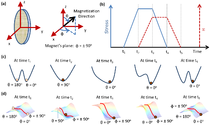
We consider that the single-domain magnetostrictive nanomagnet is shaped like an elliptical cylinder with its elliptical cross-section lying on the - plane; the major axis and minor axis are aligned along the - and -direction, respectively (see Fig. 1a). In standard spherical coordinate system, is the polar angle and is the azimuthal angle. Any deviation of magnetization from magnet’s plane (- plane, ) is termed as out-of-plane excursion. The dimensions of the major axis, the minor axis, and the thickness are , , and , respectively. So the magnet’s volume is . Due to this shape anisotropy, the two degenerate states and along the -direction (easy axis) can store a bit of information. The -axis is the in-plane hard axis and the -axis is the out-of-plane hard axis. Since , the out-of-plane hard axis is much harder than the in-plane hard axis.
Figure 1b shows the time-cycle of uniaxial stress (along -direction) and a magnetic field (along direction) applied on the magnetostrictive nanomagnet. The adiabatic pulses should be slow enough that magnetization follows its potential landscape and the quasistatic assumption is valid. We can write the total energy of the nanomagnet per unit volume as the sum of three energies – the shape anisotropy energy, anisotropies induced due to applied stress and asymmetry-making magnetic field (note that it is possible to replace the magnetic field by intrinsic interface coupling between polarization and magnetization in multiferroic heterostructures [53, 54]) – as follows [37]:
where
| (1) | |||||
| (2) | |||||
| (3) |
, is permeability of free space, is the saturation magnetization, is the Stoner-Wohlfarth switching field [36], is the demagnetization field [37], is the mth () component of the demagnetization factor [40] (), is the magnetostriction coefficient of the magnetostrictive nanomagnet [37], is the stress, is the Young’s modulus, is the strain that generates the stress, and is the magnetic field at time .
Note that a negative product will favor alignment of the magnetization along the minor axis (-axis) and according to our convention, in a material having positive , a sufficiently high compressive stress that can overcome the in-plane shape-anisotropic barrier will rotate the magnetization toward the in-plane hard axis (, ). This is depicted in Figs. 1c and 1d that magnetization initially starting from any of the two degenerate stable states (, state and , state with probabilities, ) comes to the in-plane hard axis at time . The initial entropy of the system at time is . However, when stress is applied between time and , the barrier separating the two stable states gets removed and the potential landscape becomes monostable in -space (at ) with entropy zero. A reduction of entropy must be dissipated as heat during this process. The reason that the barrier is removed before applying any asymmetry-making field is to make the erasure process independent of barrier height, which determines the hold failure probability and also to resist thermal fluctuations by making the monostable well deep enough.
Note that upon reaching , magnetization may situate in -space either at or at , which is a consequence of having the planar shape of the nanomagnet, however, it should not be related to -space in which the magnetization is switched. The -space does exist even at or [e.g., see Supplementary Fig. S1, where there exist two peaks at around ].
Between times and , an asymmetry-making field is applied to deterministically rotate the magnetization to state . The degree of this tilt should be sufficient enough to dissuade thermal fluctuations. Afterwards, both the stress and are removed to complete the switching process. Note that the entropy of the system at time and onwards are zero. Hence there is no minimum energy dissipation bound when magnetization traverses from time to as the dissipation can be made arbitrarily small.
The torque acting on the magnetization is derived from the gradient of potential landscape. Additionally, there is a random thermal field [, ] to incorporate thermal fluctuations [61]. Solving the stochastic Landau-Lifshitz-Gilbert equation [59, 60, 61] of magnetization dynamics analytically (see Supplementary material for details), we get the following coupled equations for and :
| (4) | |||||
| (5) | |||||
where
| (6) | |||||
| (7) | |||||
| (8) | |||||
| (9) | |||||
| (10) |
is the dimensionless phenomenological Gilbert damping parameter [62, 63, 64, 65], is the gyromagnetic ratio for electrons, is proportional to the attempt frequency of the thermal field, is the simulation time-step used, and the quantity is a Gaussian distribution with zero mean and unit variance.
The energy dissipated in the nanomagnet due to Gilbert damping can be expressed as , where is the time taken during the erasure cycle [i.e., in Fig. 1(b)], and is the power dissipated at time per unit volume given by
| (11) |
where is the torque (see Supplementary material for details) acting on the magnetization due to the gradient of potential energy [Equation (2)]. Thermal field with mean zero does not cause any net energy dissipation but it causes variability in the energy dissipation by scuttling the trajectory of magnetization.
Assuming magnetization resides in-plane () between times and , , is the stress at which the energy barrier is just removed, and , we can deduce from Equation (4) without considering thermal fluctuations (i.e., ) that
| (12) | |||||
Note that at and , the above expression is undefined or it would take exceedingly large amount of time to start exactly from and to reach exactly at since the torque acting on the magnetization at these points due the gradient of potential landscape vanishes. Fortunately, thermal fluctuations can prevent this lockjam in such circumstances. Assuming and , . This closed-form expression gives us an estimate over the time required for magnetization to reach depending on the material parameters involved.
It needs mention here that particularly in the presence of thermal fluctuations, magnetization may temporarily traverse on higher potential (not only in-plane of the nanomagnet but also out-of-plane, i.e., when ) and dissipate energy when it comes back to lower potential. A less than one degree of deflection in the out-of-plane direction can have immense consequence on magnetization dynamics. The key reason behind is that the out-of-plane demagnetization field is about a couple of orders of magnitude higher than . When the magnetization deflects out-of-plane due to torque exerted on it, an additional torque of comparatively very high magnitudes comes into play [see Equation (7)], which makes the dynamics fast. It is true that the out-of-plane excursion causes power dissipation but switching also becomes fast, so that the net energy dissipation may be smaller compared to the case when it is assumed that magnetization is confined to the magnet’s plane. Since the Landauer limit of energy dissipation is very small, we should particularly take into consideration this significant effect due to out-of-plane excursion of magnetization.
We will now analyze the magnetization dynamics between times and . Assuming and , the total energy becomes . We see that as goes from to , the minimum value of goes from to continuously following the expression .
Due to the smooth transitions of magnetization, with adiabatic pulses between times and , there is no lower bound of energy dissipation in the absence of thermal fluctuations. However, the Landauer principle remains intact since this is case and thus the energy dissipation proportional to temperature is also zero. If we incorporate random thermal fluctuations at finite temperature, magnetization will get deflected uphill in the potential landscape even with very slow ramp of pulses and will incur energy dissipation, which is subjected to Landauer bound.
3 Results
We consider the magnetostrictive nanomagnet to be made of polycrystalline Galfenol (FeGa), which has the following material properties – magnetostrictive coefficient (): +15010-6, saturation magnetization (): 8105 A/m, Gilbert damping parameter (): 0.025, and Young’s modulus (Y): 140 GPa [66, 67]. The dimensions of the nanomagnet is chosen as = 100 nm, = 90 nm, and = 6 nm, which ensures that the nanomagnet has a single ferromagnetic domain [39]. With the chosen dimensions, the Stoner-Wohlfarth switching field becomes . The values of stress (), strain (), and asymmetric field () are 60.6 MPa, 43310-6, and 0.01 T, respectively.

Figure 2 shows the magnetization dynamics when both the ramp-up and ramp-down times of stress and H field are 400 ns (Equation (12) gives a value of 400 ns). Both the results – when magnetization is assumed to be restricted on the magnet’s plane (2D assumption) and while considering full there-dimensional potential landscape – are plotted. Note that even a less than one degree deflection of magnetization out of magnet’s plane (see azimuthal angle -plots in Fig. 2b) has caused a significant change in the -dynamics due to inherent - coupling in LLG equation. The actual dynamics is quite faster than when 2D assumption is enforced. In small systems, the out-of-plane demagnetization factor is not that high compared to the - and -component (ratio is about 10 times) and since there are torques acting on the magnetization in the -direction, magnetization can easily deflect out-of-plane particularly in the presence of thermal fluctuations.

Figure 3 shows the distribution of energy dissipation at 300 K during the time interval = 100 ns to depict that the generalized Landauer principle of energy dissipation is maintained. Stochastic violation of Landauer’s bound 0.6932 due to thermal fluctuations is observed but the mean energy dissipation does respect the Landauer’s bound. In the presence of thermal fluctuations, we note that a slower ramp rate of pulse is sufficient than that for 0 K, since thermal fluctuations does a net favor to direct magnetization going downhill. The mean energy dissipation during the time interval (when magnetization traverses from towards ) is 0.07, which does not have any bound since there is no entropy loss in the system.
4 Conclusions
We have shown that Landauer limit of energy dissipation is achievable in a magnetostrictive nanomagnet. With realistic parameters and an well-accepted model, i.e., Landau-Lifshitz-Gilbert equation of magnetization dynamics, we have performed simulations and the results show that unlike the case of a particle with linear motion, the out-of-plane excursion of magnetization plays a crucial role in shaping the magnetization dynamics while achieving the Landauer limit. We hope that our finding would stimulate experimental efforts to demonstrate that the magnetostrictive nanomagnets are suitable for exploring the thermodynamic limit of energy dissipation. On applied perspective, such miniscule dissipation can be the basis of ultra-low-energy computing for our future information processing systems. Also, this can open up unprecedented applications that need to work with the energy harvested from the environment e.g., monitoring an epileptic patient’s brain to report an impending seizure by drawing energy solely from the patient’s body.
References
References
- [1] Landauer R 1961 IBM J. Res. Dev. 5 183–191
- [2] Fredkin E and Toffoli T 1982 Int. J. Theor. Phys. 21 219–253
- [3] Likharev K K 1982 Int. J. Theor. Phys. 21 311–326
- [4] Maroney O J E 2005 Stud. Hist. Phil. Mod. Phys. B 36 355–374
- [5] Merkle R C 1993 Nanotechnology 4 21
- [6] Lim J, Kim D and Chae S 1999 IEEE J. Solid-State Circuits 34 898–903
- [7] Lloyd S 2000 Nature 406 1047–1054
- [8] Maxwell J C 1871 Theory of Heat (Appleton, London)
- [9] Maruyama K, Nori F and Vedral V 2009 Rev. Mod. Phys. 81 1–23
- [10] Leff H and Rex A F 2010 Maxwell’s Demon 2 Entropy, Classical and Quantum Information, Computing vol 2 (CRC Press)
- [11] Mandal D and Jarzynski C 2012 Proc. Nat. Acad. Sci. 109 11641–11645
- [12] Szilard L 1929 Z. Phys. 53 840–856
- [13] Brillouin L 1951 J. of Appl. Phys. 22 334–337
- [14] Shannon C 1948 Bell Syst. Tech. J. 27 379–423
- [15] Landauer R 1996 Science 272 1914–1918
- [16] Neumann J V 1966 Univ. Illinois Press, Urbana, IL
- [17] Landauer R 1988 Nature 335 779–784
- [18] Bennett C H 1973 IBM J. Res. Dev. 17 525–532
- [19] Bennett C H 1982 Int. J. Theor. Phys. 21 905–940
- [20] Bennett C H and Landauer R 1985 Sci. Am. 253 48–56
- [21] Jarzynski C 1997 Phys. Rev. Lett. 78 2690
- [22] Crooks G E 1999 Phys. Rev. E 60 2721
- [23] Bustamante C, Liphardt J and Ritort F 2005 Phys. Today 58 43
- [24] Dillenschneider R and Lutz E 2009 Phys. Rev. Lett. 102 210601
- [25] Lambson B, Carlton D and Bokor J 2011 Phys. Rev. Lett. 107 010604
- [26] Sagawa T 2012 Prog. Theor. Phys. 127 1–56
- [27] Wang G M, Sevick E M, Mittag E, Searles D J and Evans D J 2002 Phys. Rev. Lett. 89 050601
- [28] Carberry D M, Reid J C, Wang G M, Sevick E M, Searles D J and Evans D J 2004 Phys. Rev. Lett. 92 140601
- [29] Toyabe S, Sagawa T, Ueda M, Muneyuki E and Sano M 2010 Nat. Phys. 6 988–992
- [30] Sagawa T and Ueda M 2009 Phys. Rev. Lett. 102 250602
- [31] Dillenschneider R and Lutz E 2010 Phys. Rev. Lett. 104 198903
- [32] Sagawa T and Ueda M 2010 Phys. Rev. Lett. 104 198904
- [33] Allahverdyan A E and Nieuwenhuizen T M 2001 Phys. Rev. E 64 056117
- [34] Hilt S, Shabbir S, Anders J and Lutz E 2011 Phys. Rev. E 83 030102
- [35] Bérut A, Arakelyan A, Petrosyan A, Ciliberto S, Dillenschneider R and Lutz E 2012 Nature 483 187–189
- [36] Stoner E C and Wohlfarth E P 1948 Phil. Trans. Roy. Soc. A (London) 240 599–642
- [37] Chikazumi S 1964 Physics of Magnetism (Wiley New York)
- [38] Brown W F 1968 J. Appl. Phys. 39 993
- [39] Cowburn R P, Koltsov D K, Adeyeye A O, Welland M E and Tricker D M 1999 Phys. Rev. Lett. 83 1042–1045
- [40] Beleggia M, Graef M D, Millev Y T, Goode D A and Rowlands G E 2005 J. Phys. D: Appl. Phys. 38 3333–3342
- [41] Skumryev V, Stoyanov S, Zhang Y, Hadjipanayis G, Givord D and Nogués J 2003 Nature 423 850–853
- [42] Kilby J S 2000 Nobel Lecture in Physics (The Nobel Foundation, Sweden)
- [43] Moore G E 1998 Proc. IEEE 86 82–85
- [44] Borkar S 1999 IEEE Micro 19 23–29
- [45] Eerenstein W, Mathur N D and Scott J F 2006 Nature 442 759–765
- [46] Roy K, Bandyopadhyay S and Atulasimha J 2011 Appl. Phys. Lett. 99 063108
- [47] Roy K, Bandyopadhyay S and Atulasimha J 2011 Phys. Rev. B 83 224412
- [48] Roy K, Bandyopadhyay S and Atulasimha J 2013 Sci. Rep. 3 3038
- [49] Roy K, Bandyopadhyay S and Atulasimha J 2012 J. Appl. Phys. 112 023914
- [50] Roy K 2013 SPIN 3 1330003
- [51] Roy K 2013 Appl. Phys. Lett. 103 173110
- [52] Roy K 2014 Appl. Phys. Lett. 104 013103
- [53] Fechner M, Zahn P, Ostanin S, Bibes M and Mertig I 2012 Phys. Rev. Lett. 108 197206
- [54] Roy K 2014 J. Phys. D: Appl. Phys. 47 252002
- [55] Tiercelin N, Dusch Y, Klimov A, Giordano S, Preobrazhensky V and Pernod P 2011 Appl. Phys. Lett. 99 192507
- [56] Lei N, Devolder T, Agnus G, Aubert P, Daniel L, Kim J, Zhao W, Trypiniotis T, Cowburn R P, Daniel L, Ravelosona D and Lecoeur P 2013 Nature Commun. 4 1378–1–1378–7
- [57] Kim H K D, Schelhas L T, Keller S, Hockel J L, Tolbert S H and Carman G P 2013 Nano Lett. 13 884–888
- [58] Jin T, Hao L, Cao J, Liu M, Dang H, Wang Y, Wu D, Bai J and Wei F 2014 Appl. Phys. Express 7 043002
- [59] Landau L and Lifshitz E 1935 Phys. Z. Sowjet. 8 101–114
- [60] Gilbert T L 2004 IEEE Trans. Magn. 40 3443–3449
- [61] Brown W F 1963 Phys. Rev. 130 1677–1686
- [62] Callen H B 1958 J. Phys. Chem. Sol. 4 256–270
- [63] Kamberský V 2007 Phys. Rev. B 76 134416
- [64] Gilmore K, Idzerda Y U and Stiles M D 2007 Phys. Rev. Lett. 99 027204
- [65] Hickey M C and Moodera J S 2009 Phys. Rev. Lett. 102 137601
- [66] Brintlinger T, Lim S H, Baloch K H, Alexander P, Qi Y, Barry J, Melngailis J, Salamanca-Riba L, Takeuchi I and Cumings J 2010 Nano Lett. 10 1219–1223
- [67] Lou J, Reed D, Pettiford C, Liu M, Han P, Dong S and Sun N X 2008 Appl. Phys. Lett. 92 262502