Gradient-based Constrained Optimization Using a Database of Linear Reduced-Order Models
Abstract
A methodology grounded in model reduction is presented for accelerating the gradient-based solution of a family of linear or nonlinear constrained optimization problems where the constraints include at least one linear Partial Differential Equation (PDE). A key component of this methodology is the construction, during an offline phase, of a database of pointwise, linear, Projection-based Reduced-Order Models (PROM)s associated with a design parameter space and the linear PDE(s). A parameter sampling procedure based on an appropriate saturation assumption is proposed to maximize the efficiency of such a database of PROMs. A real-time method is also presented for interpolating at any queried but unsampled parameter vector in the design parameter space the relevant sensitivities of a PROM. The practical feasibility, computational advantages, and performance of the proposed methodology are demonstrated for several realistic, nonlinear, aerodynamic shape optimization problems governed by linear aeroelastic constraints.
Keywords:
constrained optimization, flutter , gradient-based optimization , interpolation on a matrix manifold , model reduction , parameter sampling1 Introduction
Partial Differential Equation (PDE)-based constrained optimization problems arise in numerous engineering applications including automatic design, optimal control, and inverse identification. In practice, such problems are typically solved using a Nested ANalysis and Design (NAND) approach, which incurs the solution of many instances of the constraining parametric PDE, for different sampled parameter vectors in the design parameter space denoted here by . In many industrial settings, such a PDE may model, for example, a Computational Fluid Dynamics (CFD) or Computational Structural Dynamics (CSD) problem, its discretization is high-dimensional and therefore computationally intensive, and hence its enforcement can represent a significant fraction of the total cost of the optimization problem. Of course, this situation is exacerbated when the optimization problem of interest is constrained by multiple such PDEs. For this reason, PDE-constrained optimization problems are often solved using a less computationally intensive surrogate model such as, for example, a set of response surfaces for some Quantities of Interest (QoIs), or a Projection-based Reduced-Order Model (PROM).
In general, a PROM seeks an approximate solution of the underlying High-Dimensional Model (HDM) within a subspace of the high-dimensional state space that is spanned by a Reduced-Order Basis (ROB) [1, 2]. In the context of an optimization problem, an HDM is typically a -parametric HDM, where is a design parameter vector, and denotes the dimension of the design parameter space . It is well-known that a PROM constructed for a specific design parameter vector , which is referred to in this paper as a pointwise PROM, does not necessarily perform well at another design parameter vector in this space (for example, see [3, 4]). To adress this issue, at least three approaches have been proposed so far.
In the first approach, a global ROB is constructed offline such that its associated PROM is accurate in the entire design parameter space, or at least a large region of this space [5, 6, 7]. A drawback of this approach, particularly for high-dimensional design parameter spaces, is that it may lead to a ROB that is prohibitively large, or sufficiently large to offset the computational advantages of the associated PROM. For nonlinear problems – in this context, the discretized nonlinear PDE constraints – the concept of a cluster of local, low-dimensional ROBs proposed in [8] addresses this issue. In this concept, locality refers to a region of the solution manifold, and the most appropriate local ROB is selected to approximate the solution when it evolves on its manifold.
Unlike the first approach which is comprehensive, the second approach was motivated primarily by optimization problems. In this approach, an initial ROB is progressively adapted so that it remains accurate not necessarily in the entire design parameter space, but in those regions of this space that are visited by the optimization algorithm [9, 10, 11, 12]. Specifically, as new parameter vectors are queried by the optimizer in the design parameter space, additional solution snapshots are computed only when needed to maintain accuracy, and the dimension of the PROM is adjusted to incorporate the information gathered from these snapshots. This approach is suitable when the traditional offline-online computational framework is not particularly advantageous, and the minimization of the overall computational cost is instead preferred. On the other hand, it is not necessarily advantageous when the offline-online approach is desired, and the objective is to accelerate the execution of the online phase.
For linear problems – and in the context of this paper, specifically for the discretized linear PDE constraints – the parameter dependence of a PROM associated with a -parametric HDM can be addressed using the concept of a database of PROMs introduced in [13, 14]. This approach can be summarized as follows. First, the design parameter space of interest is sampled offline using an appropriate greedy procedure, and a linear, pointwise PROM is constructed at each sampled design parameter vector using any preferred model reduction technique. Then, at each queried but unsampled design parameter vector, a PROM is constructed by interpolating the pre-computed PROMs on one or multiple matrix manifolds that characterize them. For linear problems, this approach is attractive for two reasons: the dimension of each pointwise PROM can be kept small while maintaining local accuracy, due to the restriction of the scope of such a PROM to a single parameter vector in the design parameter space (and perhaps a relatively small neighborhood); and the aforementioned interpolation on matrix manifolds can be performed in real time.
This paper focuses on the family of constrained optimization problems where the objective function may be linear or nonlinear but is time-independent, and the PDE constraint – and in the case of multiple PDE constraints, at least on of them – is linear and its discretization is high-dimensional. For such problems, which abound in engineering applications, the concept of a database of pointwise, linear PROMs is particularly attractive when multiple optimization instances must be carried out as in robust optimization, multi-objective optimization, and global optimization with multiple initial solutions. The work described here advances the state of the art of this concept, particularly for the solution of the aforementioned class of PDE-constrained optimization problems by a gradient-based NAND approach. Specifically, it contributes a parameter sampling procedure based on a saturation assumption for the construction of a cost-efficient PROM database. It also contributes a novel algorithm for interpolating the sensitivities of a pointwise, linear PROM with respect to parameter variations. Finally, it demonstrates the potential of the concept of a database of pointwise, linear PROMs equipped with these contributions for the identified class of applications. For this last purpose, it reports on the application of the proposed computational framework to the aerodynamic shape optimization of a nonlinear aeroelastic wing under a linear stability (flutter) constraint – a problem which is normally untractable when linearized CFD and CSD models are preferred for representing the PDE constraint.
2 PDE-Constrained Optimization
2.1 Problem formulation
Consider a time-independent but otherwise general PDE-constrained optimization problem, where the objective function may be linear or nonlinear and at least one of the parametric PDE constraints is linear. This problem may be also governed by additional linear or nonlinear algebraic constraints. The main objective of this paper is to present a computational framework for accelerating, in this context, the enforcement of any parametric, linear, PDE constraint whose discretization is high-dimensional. For simplicity, but without any loss of generality, assume that the optimization problem contains only one such PDE constraint (the extension of the proposed computational framework to multiple parametric, linear, PDE constraints is straightforward).
The general form of a discretized, time-independent, -parametric, linear PDE can be written as
| (1) |
where: the design parameter vector is referred to throughout the remainder of this paper as the parameter “point” in , and are the governing parametric matrix and right-hand side arising from the discretization of this PDE by degrees of freedom (dof)s; and denotes its parametric solution. The parameter point may represent, for example, the material properties, shape design parameters, or boundary conditions of a physical system of interest.
For the sake of simplicity, it is also assumed here and in the remainder of this paper that when is varied, the size and topology of the computational mesh underlying the discrete equation (1) remain unchanged. The extension of the computational framework presented in this paper to the case where this size and topology vary when is varied can be performed using the computational approaches presented in [15].
The general PDE-constrained optimization problem outlined above can be formulated as follows
| (2) |
where: denotes the objective function and is assumed here for simplicity to be a scalar function; is the -dimensional solution vector of the set of discretized nonlinear PDEs that may be present or absent from (2); and is a general set of linear and/or nonlinear algebraic constraints including, for instance, linear constraints on and/or or box constraints on .
Because this paper focuses on the NAND solution approach, problem (2) is viewed here as an optimization problem defined over the parameter point only; the state vectors and are considered as functions of that are implicitly defined by the discretized PDE constraints. When the optimizer queries a value of , an appropriate PDE solver is applied to compute each of and in a nested fashion. This is in contrast to the solution of problem (2) by the Simultaneous ANalysis and Design (SAND) approach, where the state variables of (2) are considered in this case as optimization parameters.
REMARK. While the computational framework proposed in this paper for accelerating the enforcement of the discretized, parametric, linear PDE constraint is described in the context of the solution of problem (2) by the NAND approach, it is equally applicable in the context of the solution of this problem by the SAND approach. However, its performance may not scale well with the substantially larger number of optimization parameters that is typically encountered in the latter case.
2.2 Gradient-based optimization
Because the discretized PDE constraints introduced above may lead to large-scale systems of equations, a gradient-based method is preferred for the solution of problem (2). To this end, this section reviews the computation of the relevant gradients, in order to keep this paper as self-contained as possible.
Let
and
| (3) |
A gradient-based optimization algorithm incurs the computation of the first derivatives of the objective function , and those of the constraints , . Let denote the generic representation of , any constraint , and any QoI whose derivatives with respect to the components of the parameter point must be computed. Using the chain rule, the following relations can be derived
| (4) |
For a given , the computation of the partial derivatives and is straightforward. On the other hand, the computation of warrants some attention.
The differentiation of the discretized, parametric, PDE constraint (3) with respect to any parameter component can be written as
which leads to
| (5) |
The differentiation of the discretized, parametric, linear constraint (1) with respect to any parameter component leads to the following linear system of equations governing the sensitivities of
These state vector sensitivities can be used to compute the gradients of the objective function and constraints. Indeed, substituting the solution of (5) into (4) leads to
| (6) |
which can also be written as
| (7) |
where the superscript denotes here and in the remainder of this paper the transpose operation. Equations (6) and (7) describe the direct and adjoint approaches for computing the set of sensitivities , respectively:
- 1.
- 2.
In the adjoint approach, the adjoint vector is first computed by solving the linear system of equations for , then all sensitivities are computed using (7).
The direct and adjoint approaches require and “solves”, respectively. Hence, if , the direct approach is preferrable; otherwise, the adjoint approach is preferrable.
Using the gradients computed above, problem (2) can be solved, for example, by a nonlinear optimization algorithm such as Sequential Quadratic Programming (SQP) [16] equipped with a quasi-Newton approximation of the Hessian matrix, the trust-region method [17], or the interior-point method [18]. In either case, the treatment of the discretized PDE constraints is computationally intensive. For example, computing the sensitivities of the linear PDE’s state vector with respect to the optimization parameters requires the solution of the linear system of equations (1) and that of another, large-scale linear system of equations of size . To significantly reduce this cost, model reduction can be applied to (1), and reduced-order versions of and , , can be computed instead of their high-dimensional counterparts.
3 Parametric model order reduction
Again, the focus of this paper is on accelerating the solution of the optimization problem (2), in the case where the discretized, parametric, PDE constraint (1) is high-dimensional. In this case, solving the optimization problem (2) can be prohibitively expensive. For this purpose, model reduction is applied to the discrete system of linear constraints in (3) in order to reduce its dimension, which reduces the cost of enforcing these constraints and therefore reduces the cost of solving problem (2).
3.1 Projection-based model order reduction and representation
Projection-based model order reduction reduces the dimension of a -parametric HDM such as (1), which governs the state vector , by performing the subspace approximation
| (8) |
where is a right ROB of dimension , and is a vector of generalized coordinates referred to as the reduced-order state vector. The notation emphasizes that is a pointwise ROB – that is, a ROB constructed at the parameter point – rather than a global ROB constructed to deliver accurate subspace approximations at any parameter point in the design parameter space. Typically, is constructed using the Proper Orthogonal Decomposition (POD) method of snapshots [2], which can be summarized as the collection of solution snapshots into a matrix, followed by the compression of this matrix using the Singular Value Decomposition (SVD) algorithm (see Algorithm 1).
Substituting (8) into (1) and pre-multiplying the resulting system of equations by , where is known as the left ROB associated with the right ROB , transforms this system into a square counterpart and leads to the parametric, linear, Petrov-Galerkin PROM
| (9) |
This PROM can be described by the low-dimensional matrix , the low-dimensional vector , and therefore the dublet . If , this PROM becomes a Galerkin PROM.
The sensitivities of the reduced-order state vector with respect to the parameter components , , can be computed by following the same approach described in Section 2.2. In this case, this approach entails the computation of the reduced-order sensitivity matrices and sensitivity vectors and , respectively, . It follows that the PROM (9) and its associated reduced-order sensitivity equations can be collectively represented by the tuple of low-dimensional operators
| (10) |
In summary, the subspace approximation (8) transforms the original constrained optimization problem (2) into the PROM-constrained optimization problem
| (11) |
where the discretized, parametric, linear PDE constraint and its associated sensitivity equations are low-dimensional. Just like the original constrained optimization problem (2), problem (11) can be solved using any preferred, gradient-based optimization algorithm.
3.2 Concept of a database of pointwise linear PROMs and associated sensitivities
As stated in Section 1, a PROM constructed at a parameter point does not necessarily perform well at a different parameter point in this space. Addressing this issue by constructing a new PROM at each newly queried parameter point is computationally inefficient, as it entails: the computation of new solution snapshots at the parameter point ; the compression of these snapshots using, for example, the SVD algorithm in order to compute a new right ROB ; and performing additional matrix-matrix and matrix-vector computations to compute, in the context of this paper, the tuple representing the linear PROM at the parameter point .
An alternative methodology for addressing efficiently the parameter dependence of a linear PROM based on the concept of a database of reduced-order information was proposed and developed in [19], and more recently refined in [15]. It consists in: constructing offline a database of pointwise, linear PROMs; equipping this database with a family of algorithms for interpolation on matrix manifolds [20, 13, 14]; and applying these algorithms online to build in real time a PROM at a queried but unsampled parameter point . In the context of the parametric, linear PROM (9), this offline-online methodology can be described as follows:
- 1.
Offline
- (a)
Sample parameter points in the given design parameter space .
- (b)
At each sampled parameter point , construct a pointwise, linear PROM .
- (c)
Store the set of pre-computed linear PROMs in a database (in practice, the derivatives and need not be stored, because they can be computed online as explained in Section 5).
- (a)
- 2.
Online
For each queried but unsampled parameter point , construct a pointwise, linear PROM as follows:
- (a)
For each reduced-order quantity in , identify à priori a matrix manifold where it lies, for example, by identifying the most important algebraic properties characterizing this reduced-order quantity.
- (b)
Interpolate in real time the pre-computed reduced-order quantities on their identified manifolds, at the queried but unsampled parameter point .
- (a)
In order to extend the scope of this concept of a database of pointwise, linear PROMs to the real-time solution of the constraint equation (1), in view of accelerating the solution of the optimization problem (2), the state of the art of this concept is next advanced as follows. First, a computationally efficient parameter sampling procedure based on a saturation assumption is described. Then, a novel algorithm for interpolating in real time the sensitivities of a pointwise, linear PROM with respect to parameter variations is presented.
4 Parameter sampling using a residual-based error indicator
The typical construction of an -point database for the purpose of supporting the concept of interpolation on matrix manifolds, which addresses the parameter dependence of a linear PROM, is guided by a parameter sampling procedure that selects the parameter points in the design parameter space where to pre-compute linear PROMs of interest. Specifically, such a procedure should lead to a database that has the smallest possible size , in order to minmize as much as possible the computational cost of the offline stage. It should also populate this database in a manner that delivers interpolation accuracy in the entirety of – that is, .
Parameter sampling procedures can be classified in two categories: non-adaptive procedures that sample the given design parameter space a priori; and adaptive, error-informed procedures that incorporate a feedback in the sampling process. Non-adaptive parameter sampling procedures are typically easier to implement. Adaptive counterparts however can be expected to perform better at producing databases that satisfy the desiderata outlined above.
The simplest non-adaptive parameter sampling procedure is perhaps the so-called Full Factorial (FF) sampling procedure, which samples the given design parameter space on an -dimensional grid. In principle, this grid can be made sufficiently fine to deliver accurate approximations such as those to be performed here using interpolation on a matrix manifold. However, the FF sampling procedure rapidly becomes unfeasible, as the number of parameter points it requires for achieving accuracy grows exponentially with . The alternative Latin Hypercube Sampling (LHS) procedure, which is a non-adaptive but sparse procedure, scales only linearly with . However, because it has no explicit awareness of where the approximated solution will be inaccurate, it typically leads to oversampling when attempting to meet the aforementioned accuracy desideratum.
It follows that for high-dimensional design parameter spaces, an adaptive approach where the parameter points are sampled in an incremental manner and the location of the next sampled parameter point is identified by drawing information from the already sampled parameter points is often necessary. Such an approach is typically iterative and referred to as a greedy procedure. It initializes the construction of the database by populating it with one or a small number of parameter points located, for example, in the center of and/or on its boundaries. At each iteration, it considers a set of candidate parameter points for sampling and selects that parameter point where some error estimator or indicator is maximized [7, 21, 22, 23, 24, 25, 26]. After greedy iterations, it produces a database that can be characterized as follows
where denotes the set of candidate parameter points in the design parameter space . This set can be fixed throughout the iterations or refreshed at each iteration, but in any case, should be chosen large enough to faithfully represent . The iterations performed by such a greedy procedure are terminated when the error estimator or indicator falls below a specified threshold, or the pre-set maximum size of the database or maximum run-time allocated for the execution of the procedure has been reached.
The most pertinent error for an adaptive sampling procedure is the true error , where and denote the solutions computed at the candidate parameter point of the HDM and PROM problems constructed and interpolated at , respectively, and is an approximation of that can be computed in real time (see Section 4.2). However, whereas interpolating the PROMs, solving the reduced-order problems, and reconstructing the corresponding high-dimensional solutions at the set of candidate parameter points is feasible, because each of these operations can be performed relatively fast if not in real time, the direct computation of the high-dimensional solutions for the entire set is typically prohibitively expensive. Consequently, the true error is replaced in practice by: an estimation of this error that is based on a proven error bound, when such a bound is available; or by an error indicator otherwise. Error bounds are known for the solutions of some relatively simple elliptic [27, 26], parabolic [23], and hyperbolic [28] PDEs, as well as for the solutions of some simple linear time-invariant systems [29]. However, these bounds typically require the computation of an inf-sup constant, which is seldom a simple task, and are not usually tight [30]. For this reason, computationally feasible error indicators based on some norm of a relevant residual evaluated using the reconstructed high-dimensional solution are used instead [21, 22]. In the context of this paper, such an error indicator can be expressed as , where is defined in (2). Nevertheless, even the computation of such error indicators can rapidly become overwhelming when becomes very large, for example, because the dimension of the design parameter space is increased. One approach for addressing this issue is to reduce as much as possible the number of parameter points that must be sampled to achieve the desired accuracy – that is, to minimize as much as possible the size of the database . To this end, an accelerated parameter sampling procedure based on an appropriate saturation assumption is proposed next.
4.1 Accelerated parameter sampling procedure based on a saturation assumption
Here, the set of candidate parameter points in the design parameter space , , is fixed throughout all iterations of the greedy procedure. In this case, this parameter sampling procedure can be further accelerated by using a saturation technique where previous evaluations of the error indicator are used to prevent, whenever possible, unnecessary additional evaluations of this indicator. This is possible if the accuracy of the database can be assumed to increase only to a certain extent as more parameter points are sampled, as this assumption makes it possible to omit the evaluation of the error indicator at some parameter points.
The incorporation of a saturation assumption in a greedy procedure was first proposed in [24]. Here, the efficiency of this technique is further improved by applying it at each -th iteration of the greedy procedure not to , but to a random subset of . Specifically, a fixed number of parameter points are randomly selected in at each greedy iteration to assess the accuracy of the database being constructed, and a saturation constant is defined as follows.
Definition 1.
Saturation Constant
Let denote an error indicator depending on the design parameter vector and the database . Let also
denote a sequence of nested databases – that is, a set of databases satisfying for all . The saturation constant is defined
as
| (12) |
From the above definition, it follows that: , for all ; and implies that for all . In other words, strictly decreases as more parameter points are sampled during the construction of the database. Similarly, implies a monotone decrease in as the number of sampled parameter points is increased during the construction of the database. If , may increase at some parameter point for certain iterations of the greedy procedure.
Now, consider the additional two definitions:
- 1.
Let denote the most recently computed error indicator at the candidate parameter point , where is a subset of randomly selected during the -th iteration of the greedy procedure. Note that because of the randomness aspect of the construction of the subset of candidate parameter points , might not have been selected at iteration for error indication. Hence in general, . Consequently, if was not previously selected for computing the error indicator, is set to .
- 2.
The following definition is associated with a subiterative process within the -th iteration of the greedy procedure. Let denote the current maximum indicated error at subiteration of iteration of the greedy procedure, where one error indication is computed at a candidate parameter point in . This iterative maximum indicated error is computed as follows
where also denotes a local indexing of a candidate parameter point within , and denotes the corresponding global indexing of this candidate parameter point within .
Based on the two above definitions and that of the saturation constant (12), it follows that if , then is guaranteed to be less than prior to the evaluation of the error indicator at . This is because , due to the definition of the saturation constant. Hence, it is not necessary to evaluate if . This implies that the simple inequality check between and , whose values are readily available, can avoid some unnecessary evaluations of the error indicator. Then, convergence of the greedy procedure can be monitored as follows. A check is performed to verify whether or not, where is a specified threshold tolerance for assessing the accuracy of the constructed database. For this purpose, the error indicator is evaluated at all parameter points of a larger subset of of size that is also randomly selected. If holds for this larger subset of candidate parameters, the greedy procedure is terminated.
In general, the value of is set to 1 or 2: 1 for an aggressive approach; and 2 for a conservative approach.
Algorithm 2 summarizes the greedy procedure for parameter sampling equipped with the saturation technique.
Input: A set of candidate parameter points , its size , a tolerance , a saturation constant , and two sizes
and for the two subsets of to be randomly selected at each greedy iteration
Output: PROM database
4.2 Computation of the residual-based error indicator
To complete the description of the greedy parameter sampling procedure proposed in this paper for guiding the construction of a database of linear, pointwise PROMs, it remains to discuss one subtlety regarding the practical computation of a residual-based error indicator such as
| (13) |
where all quantities appearing in (13) have been defined in the introduction part of Section 4. Note that neither the right ROB nor the left counterpart is part of the definition of the tuple representing the linear PROM constructed or reconstructed at the parameter point . Note also that the computational complexity of the construction of a ROB such as , for , scales with the dimension of the HDM: therefore, the construction of such a ROB at each candidate parameter point is not feasible. Instead, a reasonable approximation of is sought-after here. For this purpose, computing by interpolating on the Grassman manifold [20] the pre-computed ROBs at the previously sampled parameter points, which could be stored in this case in the database , is feasible, has been shown in [20] to deliver a good level of accuracy even in the context of a sparsly populated database , but unfortunately requires the solution of an auxiliary problem whose computational complexity scales with the dimension of the HDM (see [20] for details). Hence, given that in the context of a greedy procedure the level of accuracy of an approximation is not paramount for the selection among the elements of of the best parameter point to be sampled, it is proposed here to store the aforementioned pre-computed ROBs in and reconstruct for each using a constant extrapolation procedure based on the nearest sampled parameter point . This approach for computing , for each , leads to a procedure for constructing the database of interest that can be summarized as follows
This approach is not only feasible, but also computationally efficient.

5 Interpolation on a matrix manifold
Suppose that an -point database is constructed as described above, for the purpose of accelerating the solution of the reduced-order optimization problem (11) by a gradient-based algorithm. At some point of the optimization process, such algorithm may query an unsampled parameter point . Here, the idea is to construct in real time at the tuple representing the linear PROM at this point, by interpolating the content of .
To this end, it is first noted that the straightforward (or direct) interpolation of the operators defining – that is, the approach where each entry of each operator is interpolated independently from the others – is bound to deliver inaccurate results for the following reasons:
- 1.
Because the PROM operators stored in may have been constructed using different Petrov-Galerkin bases – that is, for , , the reduced-order operators defining the tuples may have been constructed for different generalized coordinate systems [14]. In this case, a correct interpolation requires first transforming the content of the database into one that uses a single generalized coordinate system.
- 2.
Both issues raised above can be addressed by first “rotating” the PROM operators defining each tuple in order to achieve consistency in the generalized coordinate system, then interpolating these operators on appropriate matrix manifolds [14].
5.1 Interpolation of projection-based reduced-order models
5.1.1 Enforcement of consistency
Starting from the observation that any ROB remains a basis of the same subspace after multiplication by an orthogonal matrix , the following classes of equivalence can be defined for each subspace
where denotes the set of orthogonal matrices in . Each equivalence class defines a set of bases leading to PROM operators that act in the same subspace, but use for this purpose different systems of generalized coordinates.
The corresponding classes of equivalence for the PROM operators themselves are
Hence, given a reference ROB and any other ROB of interest , the latter ROB can be transformed into an equivalent basis that uses the same system of generalized coordinates as that used by , through its right multiplication by the rotation matrix that solves the following minimization problem
This problem, which is known as the orthogonal Procustes problem, has the following analytical solution
| (14) |
where and are given by the SVD of the matrix product – that is,
The corresponding transformation of the tuple is given by
| (15) |
In summary, given an -point database where all tuples are not necessarily consistent – in the sense that they are not constructed for the same generalized coordinate system – the following procedure may be applied to transform the content of this database into an equivalent one that is consistent: first, identify a reference parameter ; then, rotate and all PROMs stored in the database using (14) and (15).
5.1.2 Logarithm and exponential maps and interpolation in the tangent space
Let
| (16) |
where (see (14)), be an -point database of consistent, linear PROMs. For each reduced-order operator contributing to the definition of a tuple representing a linear PROM – which in this case, is a reduced-order matrix – let denote the most important, known, matrix manifold on which this operator lies. For this purpose, any reduced-order vector contributing to the definition of the tuple is viewed here and throughout the remainder of this paper, where appropriate, as a single column matrix (hence, or ). Such a manifold can be identified, for example, by considering the most important algebraic property characterizing the reduced-order matrix to be interpolated (for example, symmetric positive definiteness in the case of the reduced-order mass matrix). Then, when interpolating this reduced-order matrix at a queried but unsmapled parameter point – which contributes to the interpolation of the linear PROM represented by the tuple – this property can be preserved by performing the interpolation on the identified matrix manifold . Such an interpolation is described below for a generic reduced-order matrix of the tuple , and the manifold of interest on which it lies.

Let denote a reference point on the manifold , which in this case is differentiable. Let also denote a set of additional points on the manifold located in a neighborhood of , . Here and throughout the remainder of this section, the superscript refers to . Then, is a mapping of onto the tangent space to at , . The neighborhood is a subset of defined such that the equation has a unique solution satisfying , where is known as the exponential map: it maps elements of the tangent space back onto the manifold . In other words, the scope of is such that the inverse operation of the logarithm map has a well-defined unique output. The tangent space being a vector space, any multi-variate interpolation approach () that is valid in a vector space can be used to interpolate the quantities . Let denote the outcome of such an interpolation in . Next, is mapped back onto via the exponential map to obtain the final outcome of the interpolation process, . This process is illustrated in Figure 2.
Table 1 gives the expressions of the logarithm and exponential maps for various matrix manifolds of practical importance. The reader can observe that these expressions can be evaluated in real time. Algorithm 3 summarizes the procedure of interpolation on a matrix manifold described above. Again, the reader can observe that this algorithm can be processed in real time. It can be furthermore encapsulated in the following expression
| (17) |
where denotes as before a queried but unsampled point of the parameter space , is a multi-variate interpolation operator that intervenes in the tangent space , and is the interpolated reduced-order matrix of interest. (For further details on the theory and practice of interpolation on a matrix manifold in the context of linear PROMs, the reader is referred to [14, 20].)
| Manifold | Nonsingular matrices | SPD matrices | |
Input: matrices belonging to a matrix manifold ; queried but unsampled parameter point
Output: Interpolated matrix
5.2 Interpolation of reduced-order model sensitivities
The solution of the reduced-order optimization problem (11) by a gradient-based algorithm requires the computation of the sensitivities of and with respect to the design parameters , . Two approaches can be considered for computing these sensitivities in real time, at a queried but unsampled parameter point :
- 1.
Finite differencing approach. For each parameter component , , interpolate each set of pre-computed and transformed reduced-order matrices and on an appropriate matrix manifold , at the parameter points and/or , where is the vector whose entries are zero except the -th entry which satisfies and . If the aforementioned interpolations are performed at the point or only, interpolate also each aforementioned set of reduced-order matrices on , at the parameter point . Then, approximate and using finite differencing.
- 2.
Analytical approach. For each parameter component , , interpolate each set of pre-computed and transformed reduced-order sensitivity matrices and on an appropriate matrix manifold , at the parameter point .
The first approach outlined above is known to lack robustness with respect to the choice of the small quantity . At each queried but unsampled parameter point , it incurs interpolations if first-order forward or backward differencing is adopted, and interpolations if second-order central differencing is used instead. The second approach mentioned above is independent of : it requires interpolations. Hence, it is the preferred approach. However, it requires the development of an appropriate algorithm for interpolating each set and on an appropriate matrix manifold, at , in order to approximate and , respectively (for the same reason explained above for the interpolation of the other components of the tuple ). Such an algoritm is proposed below, using the same notation as in Section 5.1.2.
First, note that each quantity , where may represent here the reduced-order matrix or the reduced-order matrix and , depends on but does not depend on the arbitrary parameter point . Hence, the partial derivative (17) with respect to an arbitrary parameter component can be computed at any arbitrary parameter point as
| (18) |
The objective of the algorithm presented here is to approximate the above partial derivative at a queried but unsampled parameter point using interpolation on a matrix manifold. To this end, Table 2 provides, for several practical and relevant matrix manifolds, the partial derivatives of the exponential map , . Note that can be computed analytically, but the evaluation of the partial derivative requires special attention. In order to compute this derivative, consider the matrix
| (19) |
In [31], it is shown that the exponential of such a matrix is the matrix
| (20) |
From (19) and (20), it follows that can be simply obtained by computing the exponential of the matrix , then extracting from its -block. This computation can be performed in real time as is a reduced-order matrix.
| Manifold | Nonsingular matrices | SPD matrices | |
Therefore, the proposed real-time algorithm for interpolating the quantity (18) on a matrix manifold, at a queried but unsampled parameter point , where may represent the reduced-order matrix or the reduced-order matrix (and therefore may represent the reduced-order sensitivity matrix or ) can be described as follows:
- 1.
Let be the matrix manifold to which belongs.
- 2.
Select a reference point on : for example, .
- 3.
Compute , .
- 4.
Compute also analytically , .
- 5.
Interpolate in the tangent space , at the point , to obtain an approximation of .
- 6.
Note that the above algorithm interpolates the values of the reduced-order sensitivity matrices , , on the same matrix manifold where Algorithm 3 interpolates the reduced-order matrix . Furthermore, this algorithm shares with Algorithm 3 most of its steps. Hence, both algorithms can be combined to interpolate on the same matrix manifold and its shape sensitivities , .
5.3 Tessellation-free approach based on adaptive least-squares radial basis functions
It remains to specify the interpolation method to be applied in the tangent space . The most important requirement for such a method is to be practical and perform well in the presence of high-dimensional parameter spaces and scattered data. Tessellation methods or related methods based on computational meshes constitute good candidates for this purpose when (for example, see [19]). However, they are impractical if not impossible when . High-dimensional parameter spaces call for mesh-free interpolation methods. An approach that is both popular and effective in this context is one that is based on radially symmetric basis functions that usually take the form of univariate functions of an Euclidean norm. Such an approach turns a multi-variate interpolation problem into one that is virtually one-dimensional, thereby simplifying the interpolation problem and guaranteeing some interesting mathematical properties.
In the context of the parameter space of dimension , a Radial Basis Function (RBF) is a real-valued function whose value at a parameter point depends only on the distance from this point to some other point called the center, so that
Popular RBFs include the Gaussian RBF characterized by , and the inverse quadratic RBF characterized by , where is a calibration scalar. In this work, linear combinations of these RBFs are proposed to approximate a QoI such as a component of the tuple of low-dimensional operators (10). The center points are chosen as usual to be the interpolation data, and therefore the interpolant can be written as
where the number of basis functions is in general less than or equal to the number sampled parameter points – that is, . The coefficients , are typically determined by solving the linear least-squares problem
where is the interpolation matrix defined by , , is the vector storing the values of each component of the tuple to be interpolated, , and therefore (see Section 5.1.2).
As already stated, the center points of the RBFs are typically chosen to be the entire set of sampled parameter points: this defines the straightforward implementation of an RBF-based interpolation method. For high-dimensional parameter spaces however, or when higher accuracy is desired, this implementation may incur an unacceptable computational cost, particularly in the context of real-time computations. Here, this cost is alleviated by focusing on the adaptive least-squares implementation [32] of an RBF-based interpolation, where a smaller, more economical interpolant is iteratively constructed. In this adaptive implementation, an initial interpolant is constructed using a small subset of points in as center points. Then, the same greedy procedure used to construct the database (see Section 4) but equipped with the interpolation error as an error indicator, is used to select additional center points for constructing the RBF interpolant. Though this process incurs the construction of several small interpolants, interpolation accuracy can be achieved using a substantially smaller number of center points than , which makes this implementation more efficient than its straightforward counterpart.
6 Applications
In this section, the proposed fast approach for gradient-based constrained optimization based on a database of linear PROMs is illustrated with two examples pertaining to the aeroelastic design optimization of the same wing, under the same linearized flutter constraint. The only difference between the two examples is the dimension of the parameter space – that is, the number of design parameters. All HDM-based computations are performed on 32 CPU cores (or simply, CPUs) of a Linux cluster. All HDM-based computations incurred by the offline construction of a PROM database are also performed on 32 CPUs. However, all PROM-based online computations are performed on a single CPU of the same cluster. In all cases, a CPU timing is computed and reported as the product of the corresponding wall-clock timing and the number of CPUs used to perform the corresponding computation.
Throughout the remainder of this section, the superscript ⋆ is dropped from (16) and any related quantity for the sake of simplicity. Instead, it is assumed that all information pre-computed offline is rotated as described in Section 5.1.1 before it is stored in a database , in order to enforce mathematical consistency.
6.1 Aeroelastic design optimization of a wing subject to a linearized flutter constraint
Flutter is one of the most important considerations in aircraft design. It is an aeroelastic instability that can be predicted by linearizing the governing fluid-structure equations of dynamic equilibrium around the steady-state equilibrium associated with the specified flight conditions, and solving an associated eigenvalue problem. When the fluid subsystem is modeled using CFD – for example, to improve fidelity in the transonic regime where shocks play an important role – the prediction process becomes very CPU intensive. For this reason, the aeroelastic design optimization of an aircraft wing under a linearized flutter constraint is a good candidate problem for the computational technology described in this paper.
6.1.1 Problem formulation and specification
To this end, the following constrained, aeroelastic, design optimization problem – formulated here for any generic aircraft wing – is considered:
| (21) | ||||||
where: and denote the lift and drag, respectively; denotes the weight of the wing, which is required to remain below an upper bound ; is the von Mises stress in the wing at the steady-state equilibrium point around which linearization is performed, and is constrained not to exceed the maximum allowable yield stress ; and are lower and upper bounds, respectively, that define bound constraints on in order to avoid unrealistic designs; is the vector of damping ratios, where each damping ratio is required to remain above a lower bound in order to avoid flutter; and , where 1 denotes the unit vector of same dimension as . Here, the flutter constraint is evaluated using a PROM database.
Two types of design parameters are considered and therefore is written as : aerodynamic shape parameters represented by the subvector , and structural parameters represented by . The aerodynamic shape parameters affect both the shape of the structure, and the fluid flow through the transmission conditions enforced at the fluid-structure interface. The parameter subvector contains the material properties of the structure as well as the internal shape parameters associated with its “dry” elements – that is, the elements of the structure that are not in contact with the external flow.
The constraints of problem (21) can be grouped into two sets, based on how they are evaluated:
- 1.
Static aeroelastic constraints that are computed using fluid and structural HDMs that are based on the three-field formulation of fluid-structure interaction problems [33, 34]. These constraints govern the weight, lift to drag ratio, and the von Mises stress. They are obtained from the solution of the governing nonlinear PDEs, which are not reduced in this paper.
- 2.
Dynamic, aeroelastic, flutter constraints, which are computed by linearizing the aforementioned HDMs around an equilibrium state [35, 36]. Here, the proposed PROM database strategy is exploited to alleviate the large computational cost associated with the computation of these constraints. Precisely, the computation of the vector of damping ratios and its sensitivities is accelerated using the PROM interpolation approach described in Section 5.
Specifically, the constrained design optimization problem (21) is considered here for a configuration of the Aeroelastic Research Wing (ARW-2) [37]. The physical dimensions and material properties of this wing, which has been built by NASA, are reported in Table 3. A detailed, Finite Element (FE), structural model of this wing is shown in Figure 3: it includes, among others, FE representations of the spars, ribs, hinges, and control surfaces of this wing. The model has a total of degrees of freedom (dofs). Air is assumed to behave as a perfect gas, and its flow around this wing is assumed to be inviscid. Hence, the fluid flow is modeled here by the Euler equations. The computational fluid domain is discretized by a three-dimensional, unstructured, CFD mesh (Figure 3) with nodes. The focus is set on a cruise condition defined by: the altitude ft where the atmospheric density is and the atmospheric pressure is ; the free-stream Mach number ; and the zero angle of attack.
| Parameter | Type/Value |
| Geometry (inches) | |
| Wingspan | 104.9 |
| Root | 40.2 |
| Tip | 12.5 |
| Material properties | |
| Skin (except flaps) | Composite materials |
| Stiffeners | Aluminum |
| E (psi) | |
| (lbf | |
| 0.32 |


For this wing, the upper bound for the von Mises stress constraint, , is set to psi, and that for the weight, , is set to lbs. Several values of the lower bound for the damping ratios, , are considered in the interval in order to study how the optimal aeroelastic design varies with this flutter threshold.
Three shape and three structural parameters are considered – that is, and . The shape parameters are the back sweep angle , the twist angle , and the dihedral angle . These parameters, which are graphically depicted in Figure 4, are constrained to have a magnitude less than 0.1 radian.
For the purpose of optimization, the stiffeners of the ARW-2 are organized in three different groups: the outer spars, the central spar, and the ribs (see Figure 5). Each of these groups contains elements with different thicknesses, but is attributed a single, collective thickness increment as an optimization parameter. Hence, the structural parameters stored in are the three thickness increments for the outer spars (), the central spar (), and the ribs (). The magnitude of each of these increments is constrained to be less than 0.01 in – which corresponds on average to 10% of the thickness of a stiffening element of the considered initial configuration of the ARW-2.


Specifically, two different instances of the design optimization problem (21) are considered in the remainder of this section for the ARW-2:
- 1.
A first instance where only the aerodynamic shape parameters are activated as optimization parameters – that is, .
- 2.
A second instance where both the aerodynamic shape and structural parameters are activated as optimization parameters – that is, .
For each instance outlined above, the performance of the model reduction approach adopted here for computing the flutter constraints and its impact on the overall performance of the NAND solution algorithm is measured relative to the performance results obtained using the HDM-based solution strategies.
6.1.2 Linearized CFD-based computational aeroelasticity and model order reduction
A high-fidelity, nonlinear, CFD-based fluid-structure (or aeroelastic) system can be described by a three-field Arbitrary Lagrangian Eulerian (ALE) formulation [33, 34] that treats the moving CFD mesh as a pseudo-structural system [38]. After semi-discretization, linearization of the governing semi-discrete equations about a fluid-structure equilibrium state [35, 36], and elimination from these equations of the CFD mesh position vector, this formulation leads to the following system of linear Ordinary Differential Equations (ODEs)
| (22) | |||||
| (23) |
where: a dot denotes a derivative with respect to time ; is the diagonal matrix of cell volumes in the CFD mesh, and is the dimension of the semi-discretized fluid subsystem; denotes the conservative fluid state vector; is the vector of structural displacements of dimension ; and denote the Jacobians of the numerical fluid fluxes with respect to and , respectively; is the Jacobian of the numerical fluid fluxes with respect to the fluid mesh velocity; is the mass matrix associated with the FE representation of the structural subsystem; and are the FE damping and stiffness matrices, respectively; and denotes the Jacobian of the aerodynamic forces with respect to and acts on the “wet” surface of the structure – that is, the fluid-structure interface.
First, the dimensionality of the structural subsystem is reduced using modal truncation. For this purpose, a ROB , where depends on the parameter vector , is constructed using the first modes of the structural subsystem. Then, the subspace approximation
where denotes the vector of generalized coordinates associated with the modal approximation, is performed. Finally, Equation (23) is reduced by Galerkin projection onto to obtain
where and is the diagonal matrix of eigenvalues associated with the eigenmodes.
The dimensionality of the fluid subsystem is reduced using the POD method in the frequency domain [39]. Specifically, a ROB is constructed using Algorithm 4. Note that by construction, this global ROB satisfies the orthogonality condition . Next, the state vector is approximated as
where denotes the vector of generalized coordinates associated with , and Galerkin projection is performed to transform (22) into the set of reduced-order coupled linear ODEs
| (24) | |||||
| (25) |
where , , and . If needed, the stability of this resulting fluid-structure PROM can be enforced using the fast algorithm described in [40].
Input: Parameter vector ,
frequency sampling ,
structural eigenmodes ,
desired ROB dimension
Output: ROB
For simplicity, and without any loss of generality, structural damping is neglected throughout the remainder of this section – that is .
Given that and , the reduced-order eigenvalue problem
| (28) |
can be solved in real-time, for any specified value of , to obtain the eigenpairs . For each computed eigenvalue , which can be complex-valued, the corresponding damping ratio is defined as
| (29) |
where and are the real and imaginary part of , respectively.
During the solution of the optimization problem (21), many values of the parameter vector will be queried. For any value for which the blocks of the matrix (27) are not available in the PROM database constructed offline, the PROM interpolation method described in Section 5 is applied to construct and its sensitivities with respect to the optimization parameters block-by-block. For this purpose, Equation (28) can be identified with Equation (9) – or more specifically, the reduced-order matrix can be identified with the reduced-order matrix – even if (1) is a linear system of equations but (28) is a linear eigenvalue problem.
6.2 Offline database construction
Three different instances of the greedy procedure are applied offline to construct three different databases of coupled PROMs of the form (27) and of reduced dimensions and and compare their performances. In all three instances: the set of candidate parameter points is constructed using FF design and five points along each dimension of the parameter space, which leads to ; the convergence tolerance is set to ; and the error indicator is chosen to be the residual-based error indicator (13) with set – for this purpose, and only for this purpose – to the residual associated with the first eigenpair of the PROM matrix (27).
The three aforementioned instances differ as follows:
- 1.
Standard. In this case the residual-based error indicator is evaluated at each iteration at every candidate parameter point in .
- 2.
Random. In this case, the residual-based error indicator is evaluated at each iteration at every candidate parameter point in a random subset of size .
- 3.
Saturation. In this case, the greedy procedure is that described in Algorithm 4.1 with and . The saturation constant is set to in order to capture a fluctuation of the error at some parameter points as more of these points are sampled to refine the database of PROMs.
The performances of these databases are contrasted in Table 4 for . The reader can observe that the accelerated parameter sampling procedure based on a saturation assumption described in Section 4.1 and Algorithm 4.1 reduces the computational cost of the standard greedy procedure by a factor greater than 7.
All performance results reported in the remainder of this paper are for the database of coupled PROMs constructed using Algorithm 4.1.
| Greedy procedure | Standard | Random | Saturation |
| 125 | 125 | 125 | |
| - | 20 | 20 | |
| Number of sampled HDMs | 16 | 15 | 15 |
| Maximum Relative Indicated Error () | 4.9 | 3.9 | 4.6 |
| Total wall-clock time (hrs) | 60.9 | 12.1 | 8.4 |
| Speed-up with respect to standard greedy procedure | 1 | 5.1 | 7.3 |
6.3 Speed-up factors for one online evaluation of the flutter constraint
Table 5 compares the performance of the proposed methodology for accelerating the evaluation of a discretized, parametric, linear PDE constraint with that of the HDM-based evaluation of this constraint, for a single computation of the vector of damping ratios in problem (21). For this purpose, this computation ( and ) is carried out using the fixed-point iteration algorithm described in [41]. For the case where , the PROM database approach is shown to deliver a speed-up factor roughly equal to for the wall-clock time, and for the CPU time. For the case , the speed-up factor for the wall-clock time is roughly equal to , and that for the CPU time is slightly larger than .
| Computational model | () | () | ||||
| of CPUs | Wall-clock | CPU | of CPUs | Wall-clock | CPU | |
| time | time | time | time | |||
| HDM | 32 | 0.342 | 10.934 | 32 | 0.492 | 15.744 |
| Database of PROMs | 1 | 0.019 | 0.019 | 1 | 0.017 | 0.017 |
| Speed-up factor | 18.0 | 575.5 | 28.9 | 926.1 | ||
6.4 Speed-up factors for the solution of the optimization problem with
Table 6 summarizes the results obtained for the solution of the optimization problem (21) with and . Given the same initial shape defined by , both computational approaches based on the HDM and PROM database are found to deliver almost the same optimal design, after almost the same number of iterations. (The initial and optimized shapes of the ARW-2 are shown in Figure 6). However, Figure 7 shows that the optimization paths followed by both computational models are different. In both cases, the flutter constraint is violated initially, but satisfied at convergence to the optimal shape. After optimization, the lift to drag ratio is increased by , and the weight and maximum von Mises stresses are increased by and , respectively, without violating their respective constraints. Figure 8 shows the iteration-histories of the lift to drag ratio, minimum damping ratio, maximum von Mises stress, and weight. Again, this figure shows that the two computational models contrasted here converge to the same results, but follow different paths in general.
Table 6 also reports the CPU timing results obtained for each considered computational model. The CPU timing result reported for the offline phase of model reduction corresponds to the CPU time elapsed in constructing the PROM database using the accelerated parameter sampling procedure described in Section 4.1. The “static” constraints refer to all of the weight, von Mises, and box constraints, as well as the objective function. The flutter constraint refers as before to the constraint on the vector of damping ratios. The following observations are noteworthy:
- 1.
The CPU-based speed-up factor achieved for the online evaluation of the flutter constraint is consistent with that reported in Table 5 for a single such evaluation.
- 2.
The smaller speed-up factor achieved for the entire online phase is due to the fact that the so-called static constraints are not reduced.
- 3.
Because it requires an offline investment, the PROM database approach can be expected to deliver a (significant) speed-up factor only if this investment is amortized. As this table shows, such an investment is rarely amortized by the solution of a single problem – in this case, an optimization problem. However, it will be shown next that such an investment can be amortized if multiple optimizations are performed – for example, as in multi-start global optimization strategies.
| Design | Initial | Optimized | Optimized |
| Computational model | HDM | PROM database | |
| # of CPUs | 32 | variable | |
| (0.1,0.1,0.1) | (-0.1,-0.0814,0.1) | (-0.1,-0.0807,0.1) | |
| 10.6 | 12.2 | 12.2 | |
| Weight (lbs) | 342.6 | 357.7 | 357.7 |
| Min. | |||
| Max. (psi) | 18,731.9 | 22,139.5 | 22,139.0 |
| # of iterations | 5 | 6 | |
| # of function evaluations | 24 | 22 | |
| CPU time (hours) | |||
| Offline phase (32 CPUs) | 0 | 268.8 | |
| Online evaluation of the static constraints (32 CPUs) | 14.2 | 14.1 | |
| Online evaluation of the flutter constraint (1 CPU) | 240.5 | 0.43 | |
| Total (online) | 254.7 | 14.5 | |
| Total (offline + online) | 254.7 | 283.3 | |
| Speed-up factors based on CPU time | |||
| Speed-up factor for flutter constraint | 1 | 559.3 | |
| Speed-up factor for online phase | 1 | 17.6 | |
| Total speed-up factor | 1 | 0.7 |
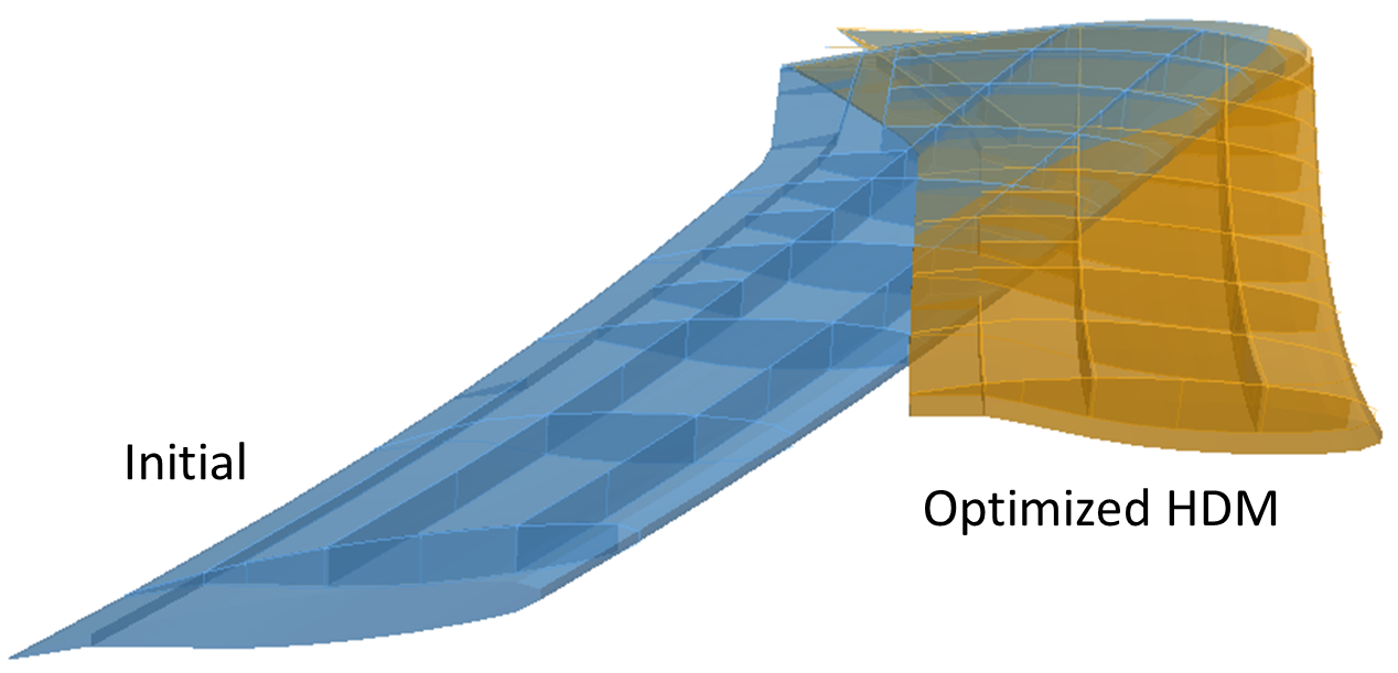


Table 7 reports the CPU timing results obtained for multiple instances of the flutter optimization problem (21), corresponding to the following nine different values of the lower bound for the damping ratios, , for the purpose of studying the influence of this flutter threshold on the optimized design. Furthermore for each damping ratio lower bound, a multi-start strategy with ten different initial points is applied in order to provide a more robust search for a global optimizer. Therefore, the performance results reported in Table 7 correspond to 90 independent optimization problems that are solved using both of the HDM and PROM database computational models. In this case, the reader can observe that:
- 1.
The proposed PROM database approach delivers a speed-up factor based on the CPU time that is equal to for the flutter constraint, and a speed-up factor based on the CPU time that is equal to for the overall online phase.
- 2.
This approach achieves a speed-up factor based on the CPU time that is equal to for the entire computations, including those incurred by the construction offline of the database of PROMs, which confirms the observation made above.
Figure 9 graphically depicts the influence of on the optimal lift to drag ratio, the optimal weight, and the maximum von Mises stress associated in each case with the optimal design. Overall, this influence appears to be minimal. Similarly, Figure 10-left shows the influence of on the minimum damping ratio associated with an optimal design.
Figure 10-right reports on the relative error associated with the computation of the minimum damping ratio using the PROM database approach, for all considered values of . It shows that in all cases, this error is significantly below the convergence threshold of adopted during the construction offline of the PROM database.
| Computational model | HDM | PROM Database |
| # of CPUs | 32 | variable |
| CPU time (hours) | ||
| Offline phase (32 CPUs) | 0 | 268.8 |
| Online evaluation of the static constraints (32 CPUs) | 2,065.1 | 755.7 |
| Online evaluation of the flutter constraints (1 CPU) | 31,813.5 | 21.8 |
| Online miscellaneous | 14.2 | 0.06 |
| Total (online) | 33,892.8 | 777.6 |
| Total (offline + online) | 33,892.8 | 1,046.4 |
| Speed-up factors based on CPU time | ||
| Speed-up factor for flutter constraints | 1 | 1,459.3 |
| Speed-up factor for online phase | 1 | 43.6 |
| Total speed-up factor | 1 | 32.4 |


6.5 Speed-up factors for the solution of the optimization problem with
Table 8 presents the performance results obtained for the solution of the optimization problem (21) with and . As in the case of three shape parameters (), both computational models based on the HDM and PROM database approaches are found to deliver almost the same optimal shape, given the same initial design. However, the two different computational models lead in this case to two slightly different optimal structural parameters. In both cases, the flutter constraint is violated initially but satisfied at convergence, and the lift to drag ratio is increased by . However, the weight is increased by in the optimal design found using the PROM database as a computational model, but is maintained almost constant in the counterpart design found by the HDM-based optimization process. The maximum von Mises stress is decreased by in the optimal design found using the PROM database computational model, and by in the counterpart design found using the HDM-based approach. Although the optimal shape parameters obtained in this case – – are similar to those obtained in the case of optimization using only the three shape parameters (see Table 6), the maximum von Mises stress experienced in this case by the optimal design is smaller than its counterpart experienced by the optimal design obtained when . This lower value is achieved by increasing the thickness of the stiffeners without violating the weight constraint. The reader can also observe that for both considered computational models, similar iteration counts and similar numbers of function evaluations are performed.
Table 8 also reports the CPU time results and associated speed-up factors achieved for this instance of the optimization problem (21). Due to the larger computational expense induced by the computation of a larger number of sensitivities, the CPU time-based speed-up factor achieved by the PROM database approach for a single evaluation of the flutter constraint and its sensitivities is substantially higher (speed-up factor = 1,154.7) than for the case where (speed-up factor = 559.3). The speed-up factor for the overall online phase of model reduction is similar however in magnitude. Again, the total speed-up factor for the combined offline and online phases is less than 1, due to the computational expense incurred by building the database. As demonstrated however for the case where , this computational overhead can be amortized and significant overall speed-up factors can be achieved when many optimization problems are solved using the same PROM database.
| Design | Initial | Optimized | Optimized |
| Computational model | HDM | PROM Database | |
| # of CPUs | 32 | variable | |
| (0,0,0) | (-0.1,-0.1,0.1) | (-0.1,-0.1,0.1) | |
| (0,0,0) | (0.1,0.1,-0.015) | (0.1,0.1,0.013) | |
| 11.3 | 12.2 | 12.2 | |
| Weight (lbs) | 349.9 | 349.8 | 366.3 |
| Min. | |||
| Max. (psi) | 20,297.1 | 18,991.9 | 18,953.3 |
| # of iterations | 6 | 5 | |
| # of function evaluations | 11 | 9 | |
| CPU time (hours) | |||
| Offline phase (32 CPUs) | 0 | 8,800 | |
| Online evaluation of the static constraints (32 CPUs) | 11.0 | 12.8 | |
| Online evaluation of the flutter constraint (1 CPU) | 173.2 | 0.15 | |
| Total (online) | 184.2 | 13.0 | |
| Total (offline + online) | 184.2 | 8,813 | |
| Speed-up factors based on CPU time | |||
| Speed-up factor for flutter constraint | 1 | 1,154.7 | |
| Speed-up factor for online phase | 1 | 14.2 | |
| Total speed-up factor | 1 | 0.02 |
7 Conclusions
A novel methodology is introduced in this paper for accelerating the solution of Partial Differential Equation (PDE)-constrained optimization problems where at least one PDE-based constraint is linear. This methodology consists in constructing offline a database of pointwise, linear, Projection-based Reduced-Order Models (PROMs), and equipping it with two essential computational technologies: an offline pre-processing algorithm for enforcing mathematical consistency among the pre-computed PROMs that are stored in the database; and an online algorithm for interpolating on matrix manifolds the pre-computed PROMs and their sensitivities at any queried but unsampled parameter point in the design parameter space. To reduce the computational overhead incurred by the construction offline of the PROM database, a parameter sampling procedure based on an appropriate saturation assumption is proposed to minimize the number of pointwise PROMs to be pre-computed and stored in the database, while maximizing the accuracy of the online interpolation of these PROMs at any queried but unsampled parameter point. The interpolation on matrix manifolds, which preserves some desirable properties of the PROMs to be interpolated and their sensitivities, incurs the standard interpolation in the tangent space to a considered manifold – which is a vector space – of some parametric quantities. It is shown in this paper that when the design parameter space is high-dimensional, such an interpolation can be practically and effectively performed using radial basis functions. A new and rigorous approach for interpolating on matrix manifolds matrix sensitivities is also presented. The PROM database approach and its peripherals are illustrated with the solution of a number of different instances of a PDE-constrained, aeroelastic, optimization problem associated with NASA’s ARW-2 wing and involving a linear, PDE-based flutter constraint. Using this problem as a background problem, it is also shown in this paper that when multiple optimizations are performed – for example, as in multi-start global optimization strategies – the computational overhead incurred by the construction offline of a PROM database can be amortized and a significant overall, CPU time-based, speed-up factor can be achieved. Finally, it is noted that given the recent work published in [42], the methodology presented in this paper is readily extendible to the case where the PDE-based optimization problem contains a combination of linear and nonlinear PDE-based constraints.
8 Appendix
Real-time computation of the sensitivity of the vector of damping ratios with respect to the optimization parameters, ,
For each eigenpair , , the differentiation of (28) with respect to , leads to
where the reduced-order matrix matrix and the associated reduced-order vector are defined in (27) and (26), respectively, is the -th right eigenvector of , is the corresponding eigenvalue, is the identity matrix, and is the -th component of the parameter vector . Multiplying (8) from the left by , where denotes the -th left eigenvector of and the superscript designates the transpose of the conjugate of a complex-valued quantity, and noting that gives
In the above result, the sensitivity matrix can be computed at any queried but unsampled parameter point in real-time, block-by-block, using interpolation on matrix manifolds as described in Section 6.1.2 (see also Table 1 and Table 2). Then, from Equation (29) and the chain rule, it follows that the sensitivity of each damping ratio with respect to any parameter component can be computed in real-time as follows
| (30) |
9 Acknowledgements
Youngsoo Choi acknowledges partial support by the office of Naval Research under Grant N00014-11-1-0707 and partial support by the Army High Performance Computing Research Center under Cooperative Agreement W911NF-07-2-0027, while in residence at Stanford University. Gabriele Boncoraglio and Charbel Farhat acknowledge partial support by the Office of Naval Research under Grant N00014-17-1-2749, partial support by the Boeing Company under Contract Sponsor Ref. 134824, and partial support by a research grant from the King Abdulaziz City for Science and Technology (KACST). Spenser Anderson acknowledges the support by the Department of Defense through the National Defense Science & Engineering Graduate Fellowship (NDSEG) Program. This document does not necessarily reflect the position of these institutions, and no official endorsement should be inferred.
10 References
References
- [1] B. Moore, Principal component analysis in linear systems: Controllability, observability, and model reduction, Automatic control, IEEE transactions on 26 (1981) 17–32.
- [2] L. Sirovich, Turbulence and the dynamics of coherent structures. part i: Coherent structures, Quarterly of applied mathematics 45 (1987) 561–571.
- [3] B. Epureanu, A parametric analysis of reduced order models of viscous flows in turbomachinery, Journal of fluids and structures 17 (2003) 971–982.
- [4] T. Lieu, C. Farhat, Adaptation of aeroelastic reduced-order models and application to an f-16 configuration, AIAA Journal 45 (2007) 1244–1269.
- [5] P. A. LeGresley, J. Alonso, Airfoil design optimization using reduced order models based on proper orthogonal decomposition, in: AIAA paper 2000-2545 fluids 2000 conference and exhibit, Denver, CO, American Institute of Aeronautics and Astronautics, Reston, Virginia, 2000, pp. 1–14.
- [6] G. Weickum, M. Eldred, K. Maute, A multi-point reduced-order modeling approach of transient structural dynamics with application to robust design optimization, Structural and Multidisciplinary Optimization 38 (2009) 599–611.
- [7] D. Amsallem, M. Zahr, Y. Choi, C. Farhat, Design optimization using hyper-reduced-order models, Structural and Multidisciplinary Optimization 51 (2015) 919–940.
- [8] D. Amsallem, M. J. Zahr, C. Farhat, Nonlinear model order reduction based on local reduced-order bases, International Journal for Numerical Methods in Engineering 92 (2012) 891–916.
- [9] M. Fahl, E. W. Sachs, Reduced order modelling approaches to PDE-constrained optimization based on proper orthogonal decomposition, in: Large-scale PDE-constrained optimization, Springer, 2003, pp. 268–280.
- [10] Y. Yue, K. Meerbergen, Accelerating optimization of parametric linear systems by model order reduction, SIAM journal on optimization 23 (2013) 1344–1370.
- [11] M. J. Zahr, D. Amsallem, C. Farhat, Construction of parametrically-robust cfd-based reduced-order models for pde-constrained optimization, in: AIAA paper 2013-2845, 21st AIAA computational fluid dynamics conference, San Diego, CA, June 26-29, 2013, American Institute of Aeronautics and Astronautics, Reston, Virginia, 2013, pp. 1–11.
- [12] M. J. Zahr, C. Farhat, Progressive construction of a parametric reduced-order model for pde-constrained optimization, International journal for numerical methods in engineering 102 (2015) 1111–1135.
- [13] D. Amsallem, J. Cortial, K. Carlberg, C. Farhat, A method for interpolating on manifolds structural dynamics reduced-order models, International journal for numerical methods in engineering 80 (2009) 1241–1258.
- [14] D. Amsallem, C. Farhat, An online method for interpolating linear parametric reduced-order models, SIAM journal on scientific computing 33 (2011) 2169–2198.
- [15] D. Amsallem, R. Tezaur, C. Farhat, Real-time solution of linear computational problems using databases of parametric reduced-order models with arbitrary underlying meshes, Journal of Computational Physics 326 (2016) 373–397.
- [16] P. E. Gill, W. Murray, M. A. Saunders, Snopt: An sqp algorithm for large-scale constrained optimization, SIAM journal on optimization 12 (2002) 979–1006.
- [17] A. R. Conn, N. I. Gould, P. L. Toint, Trust region methods, volume 1, MOS-SIAM Series on Optimizationm, SIAM, 2000.
- [18] A. Wächter, L. T. Biegler, On the implementation of an interior-point filter line-search algorithm for large-scale nonlinear programming, Mathematical programming 106 (2006) 25–57.
- [19] D. Amsallem, J. Cortial, C. Farhat, Towards real-time computational-fluid-dynamics-based aeroelastic computations using a database of reduced-order information, AIAA journal 48 (2010) 2029–2037.
- [20] D. Amsallem, C. Farhat, Interpolation method for adapting reduced-order models and application to aeroelasticity, AIAA journal 46 (2008) 1803–1813.
- [21] T. Bui-Thanh, K. Willcox, O. Ghattas, Model reduction for large-scale systems with high-dimensional parametric input space, SIAM journal on scientific computing 30 (2008a) 3270–3288.
- [22] T. Bui-Thanh, K. Willcox, O. Ghattas, Parametric reduced-order models for probabilistic analysis of unsteady aerodynamic applications, AIAA journal 46 (2008b) 2520–2529.
- [23] M. A. Grepl, A. T. Patera, A posteriori error bounds for reduced-basis approximations of parametrized parabolic partial differential equations, ESAIM: Mathematical modelling and numerical analysis 39 (2005) 157–181.
- [24] J. S. Hesthaven, B. Stamm, S. Zhang, Efficient greedy algorithms for high-dimensional parameter spaces with applications to empirical interpolation and reduced basis methods, ESAIM: Mathematical modelling and numerical analysis 48 (2014) 259–283.
- [25] A. Paul-Dubois-Taine, D. Amsallem, An adaptive and efficient greedy procedure for the optimal training of parametric reduced-order models, International journal for numerical methods in engineering 102 (2015) 1262–1292.
- [26] K. Veroy, C. Prud’homme, D. V. Rovas, A. T. Patera, A posteriori error bounds for reduced-basis approximation of parametrized noncoercive and nonlinear elliptic partial differential equations, in: Proceedings of the 16th AIAA computational fluid dynamics conference, volume 3847, pp. 23–26.
- [27] C. Prud’homme, D. V. Rovas, K. Veroy, L. Machiels, Y. Maday, A. T. Patera, G. Turinici, Reliable real-time solution of parametrized partial differential equations: Reduced-basis output bound methods, Journal of fluids engineering 124 (2002) 70–80.
- [28] B. Haasdonk, M. Ohlberger, Reduced basis method for finite volume approximations of parametrized linear evolution equations, ESAIM: Mathematical modelling and numerical analysis 42 (2008) 277–302.
- [29] B. Haasdonk, M. Ohlberger, Efficient reduced models and a posteriori error estimation for parametrized dynamical systems by offline/online decomposition, Mathematical and computer modelling of dynamical systems 17 (2011) 145–161.
- [30] D. Amsallem, U. Hetmaniuk, A posteriori error estimators for linear reduced-order models using krylov-based integrators, International journal for numerical methods in engineering 102 (2015) 1238–1261.
- [31] I. Najfeld, T. F. Havel, Derivatives of the matrix exponential and their computation, Advances in applied mathematics 16 (1995) 321–375.
- [32] G. Fasshauer, Adaptive least squares fitting with radial basis functions on the sphere, Mathematical methods for curves and surfaces (1995) 141–150.
- [33] C. Farhat, M. Lesoinne, N. Maman, Mixed explicit/implicit time integration of coupled aeroelastic problems: Three-field formulation, geometric conservation and distributed solution, International journal for numerical methods in fluids 21 (1995) 807–835.
- [34] C. Farhat, P. Geuzaine, G. Brown, Application of a three-field nonlinear fluid-structure formulation to the prediction of the aeroelastic parameters of an f-16 fighter, Computers and Fluids 32 (2003) 3–29.
- [35] M. Lesoinne, M. Sarkis, U. Hetmaniuk, C. Farhat, A linearized method for the frequency analysis of three-dimensional fluid/structure interaction problems in all flow regimes, Computer methods in applied mechanics and engineering 190 (2001) 3121–3146.
- [36] M. Lesoinne, C. Farhat, CFD-based aeroelastic eigensolver for the subsonic, transonic, and supersonic regimes, J. Aircraft 38 (2001) 628–635.
- [37] M. C. Sandford, D. A. Seidel, C. V. Eckstrom, C. V. Spain, Geometrical and structural properties of an aeroelastic research wing (arw-2), NASA Technical Memorandum 4110 (1989).
- [38] C. Farhat, C. Degand, B. Koobus, M. Lesoinne, Torsional springs for two-dimensional dynamic unstructured fluid meshes, Computer Methods in Applied Mechanics and Engineering 163 (1998) 231–245.
- [39] T. Kim, Frequency-domain Karhunen-Loeve method and its application to linear dynamic systems, AIAA journal 36 (1998) 2117–2123.
- [40] D. Amsallem, C. Farhat, On the stability of reduced-order linearized computational fluid dynamics models based on POD and galerkin projection: Descriptor vs non-descriptor forms, in: Reduced order methods for modeling and computational reduction, Springer, 2014, pp. 215–233.
- [41] D. Amsallem, D. Neumann, Y. Choi, C. Farhat, Linearized aeroelastic computation in the frequency domain based on computational fluid dynamics, arXiv:1506.07441 [physics.flu-dyn] (2015) 1–23.
- [42] K. Washabaugh, Z. J. Matthew, C. Farhat, One the use of discrete nonlinear reduced-order models for the prediction of steady-state flows past parametrically deformed complex geometries, in: AIAA paper 2016-1814, AIAA sciTech forum conference, San Diego, CA, January 4-8, 2013, American Institute of Aeronautics and Astronautics, Reston, Virginia, 2016.