Impact of momentum space anisotropy on heavy quark-dynamics in a QGP medium
Abstract
Momentum space anisotropy present in the quark and gluon distribution functions in relativistic heavy ion collisions induces Chromo-Weibel instability in the hot QCD medium created therein. The impact of the Chromo-Weibel instability on the dynamics of a heavy-quark (HQ) traversing in the QGP medium is investigated within the framework of kinetic theory by studying the momentum and temperature behavior of HQ drag and diffusion coefficients. The physics of anisotropy is captured in an effective Vlasov term in the transport equation. The effects of the instability are handled by making a relation with the phenomenologically known jet quenching parameter in RHIC and LHC. Interestingly, the presence of instability significantly affect the temperature and momentum dependences of the HQ drag and diffusion coefficients. These results may have appreciable impact on the experimental observables such as, the nuclear suppression factor, , and the elliptic flow, , of heavy mesons in heavy ion collisions at RHIC and LHC energies which is a matter of future investigation.
PACS: 25.75.-q; 24.85.+p; 05.20.Dd; 12.38.Mh
Keywords: Chromo-Weibel instability, Heavy quark transport; Quasi-particle model; Drag and diffusion; anisotropic QGP
I Introduction
The physics of the Chromo-Weibel instability [2] (non-Abelian analogue of Weibel instability [1]) during the hydrodynamic expansion of the QGP in heavy ion collisions, may play crucial role in understanding the space-time evolution and properties of quark-gluon plasma medium. The momentum anisotropy present during the hydrodynamic expansion of the QGP may induce instabilities to the Yang-Mills field (Chromo field) equations. The Weibel type of instabilities can be seen in the expanding quark-gluon plasmas, since the width of the momentum component in the direction of the expansion narrows by expansion, leading to an anisotropic momentum distribution. The instability in the rapidly expanding QGP in heavy ion collisions may lead to the plasma turbulence [3]. Recall, the plasma turbulence describes a random, non-thermal pattern of excitation of coherent color field modes in the QGP with a power spectrum similar to that of vortices in a turbulent fluid [3].
The prime goal here is to investigate the heavy quark dynamics in the presence of Chromo-Weibel instability. This could be done by first modeling the non-equilibrium momentum distribution functions that describe expanding anisotropic QGP followed by employing it to the kinetic theory description of heavy quark dynamics.
Hadrons containing HQs (, , , or ) are of great interest in investigating the properties of the QGP, since their physical properties get significantly modified while traveling through QGP. This fact has been reflected in the particle spectra at RHIC, and the LHC energies. Further, HQ thermalization time is larger than gluons and light quarks, and they do not constitute the bulk of the QGP. Since their formation occurs in the early stages of the collisions, they can travel through the thermalized QGP medium, and can retain the information about the interaction with them very efficiently. For instance, it is pertinent to ask whether a single can stay together long enough to form a bound state (say ) at the hadronization state. To address this, one requires to describe the dynamics of the HQs propagating through the QGP. Therefore, one can explore the physics of the HQ transport [4, 5, 6, 7, 8, 9, 10, 11, 12, 13, 14, 15, 16, 17, 18, 19, 20, 21] in the QGP medium as follows.The non-equilibrated HQs can travel in the equilibrated QGP medium, and one has to deal the problem within the framework of Langevin dynamics [22]. This is to say that the HQs perform random motion in the equilibrated QGP. Recall, that the QGP goes through a hydrodynamic evolution before it reaches the hadronization and subsequently the hadrons freeze-out.
The pertinent question to ask is, whether a HQs maintain equilibrium during this entire process of the space-time evolution or not. It has been observed [23] within the framework of Langevin dynamics and pQCD (perturbative QCD) that the HQs may not achieve the equilibrium in the RHIC and LHC energies.
The most important observable which encode the medium effects carried with them by the HQs while traveling in the QGP, is the nuclear modification factor, . It has been observed that their energy loss in the QGP due to gluon radiation is insufficient to describe the medium modification of the spectrum [24, 25]. Therefore, one has to look at the collisions since they have different fluctuation spectrum than radiation, and might contribute significantly as one thought off initially [26, 27]. The collisional effects can be captured well in the HQ drag and diffusion coefficients which have been calculated within weak coupling QCD by several authors. The formalism, and details are offered in Sec. IIA.
The temperature, and chemical potential, dependence of the drag and diffusion coefficient enter through the thermal distributions of light quarks and gluons. In the present calculation, we ignore the dependence in view of the fact that the QGP produced at RHIC and LHC energies at the mid-rapidity region has negligibly small net baryon density. But one has to implement the realistic QGP EoS in terms of appropriate form of the thermal distribution functions. Lattice QCD EoS may be a good choice for the description of the equilibrated QGP. Additionally, it is important to address the role of the momentum anisotropies at RHIC and LHC in influencing the dynamics of the heavy quarks in the hot QCD medium. This is the main focus of the article.
The paper is organized as follows. Section II deals with the kinetic theory formulation of HQ dynamics in the background QGP medium in terms of drag and diffusion coefficients. Sec. III, discusses the non(near)-equilibrium modeling of the degrees of freedom that describes the QGP medium in the presence of anisotropy. In Sec. IV, we present the results and related discussions. Finally, conclusions are presented in Sec. V.
II Heavy-quark drag and diffusion in the hot QCD medium
HQs play crucial role in characterizing QGP as they are produced in the early stages of the heavy-ion collisions and remain extant throughout the evolution and hence can capture the information of the entire evolution of the system. The dynamics of HQs while traveling in the QGP medium can be understood in terms of the drag and diffusion coefficients following Landau’s prescription.
II.1 Heavy Quark drag and diffusion
Let us consider the elastic interaction experienced by HQs while traversing in to the hot QCD medium. Next, we consider the process ( stands for gluon and light quarks and anti quarks).
II.2 HQ drag
The the drag coefficient, can be calculated by using the following expression [28]:
| (1) |
where is given by
| (2) |
being the statistical degeneracy of the HQ propagating through QGP. The above expression indicates that the drag coefficient is the measure of the thermal average of the momentum transfer, due to interaction of the heavy quarks with the bath particle weighted by the square of the invariant amplitude, . The factor denotes the thermal distribution of the particles in the QGP. is the momentum distribution with Bose enhancement or Pauli suppressed probability in the final state. Note that will involve three types of thermal phase space distribution functions corresponding to the gluons (), light-quarks ( up and down) and the strange quarks () and corresponding anti-quarks. Hence, jointly denote these three phase space distribution as,
| (3) |
In the presence of initial momentum anisotropy, we need to model them appropriately by first setting up the transport equation and then solving it either analytically or numerically. In the present work, we consider the linearized transport equation and capture all the effects coming from the anisotropy as the first order modification to the equilibrium distribution functions for quark-antiquark and gluons.
In view of the the above, we consider the following decomposition
for the f(q) in three sectors
| (4) |
Here .
At this stage, we need the correct modeling of equilibrium (isotropic) distribution functions (first term in the right hand side of Eq. (4) and the modifications induced by the anisotropy. This is presented in the next section.
II.3 HQ diffusion
Similar to the HQ diffusion coefficient, can be evaluated as:
| (5) |
With an appropriate choice of both the drag and diffusion coefficients can be evaluated from a single expression as follows:
| (6) |
where is the Mandelstam variable and is the triangular function. In the next section we will modeling of non-equilibrium distribution functions for a rapidly expanding plasma in the presence of small momentum anisotropy.
III Modeling momentum distribution functions for gluons and quarks
III.1 The isotropic distributions
The equilibrium modeling of the momentum distribution functions employed here is based on the quasi-particle nature of the hot QCD medium (beyond ) [30]. The quasi-particle description employed here, has been developed in the context of the recent (2+1)-flavor lattice QCD EoS [29] at physical quark masses. There are more recent lattice results with the improved actions and refined lattices [31], for which we need to re-look the model with specific set of lattice data specially to define the effective gluonic degrees of freedom. Therefore, we will stick to the set of lattice data utilized in the model described in [30]. Here, form of the equilibrium distribution functions, (this notation will be useful later while writing the transport equation in both the sector in compact notations), describing the strong interaction effects in terms of effective fugacities can be written as.
| (7) |
where , denotes the mass of the strange quark(which we choose to be ), and denotes inverse of the temperature.
We use the notation for gluonic degrees of freedom, for light quarks, for the strange quark for . As we are working at zero baryon chemical potential, therefore quark and antiquark distribution functions are the same.= Since the model is valid in the deconfined phase of QCD (beyond ), therefore, the mass of the light quarks can be neglected as compared to the temperature. As QCD is a gauge theory so for our analysis.
Note that the effective fugacities () are not merely a temperature dependent parameter which encodes the hot QCD medium effects. They lead to non-trivial dispersion relation both in the gluonic and quark sectors as,
| (8) |
and this lead to the new energy dispersions for gluons (), light-quark antiquarks (), and strange quark-antiquarks. A detailed discussions of the interpretation and physical significance of , and , we refer the reader to [30]. There are other quasi-particle descriptions in the literature, those could be characterized as, effective mass models [32, 33], effective mass models with gluon condensate [34], and effective models with Polyakov loop [35]. Our model is fundamentally distinct from all these models. Another crucial point is regarding the definition of the energy momentum tensor, . As described in [36], in the presence of non-trivial temperature dependent energy dispersion (as in all these quasi-particle models), we need to modify the definition of the so that the trace anomaly effects in QCD can be accommodated in the definition. The modified for the effective mass models is obtained in [36], and for the current model in [37].
III.2 Chromo-Weibel instability and anomalous transport: Dupree-Vlasov equation
Recall, the momentum anisotropy present in quark and gluon momentum distribution functions induces instability in the Yang-Mills equations in similar way as Weibel instability in the case of Electromagnetic plasmas. This instability while coupled with the rapid expansion of the QGP leads to anomalous transport and modulates the transport coefficients of the plasma substantially. This fact is realized by Dupree in the case of EM plasmas in 1954 [38] and later generalized for the non-Abelian plasmas in [3, 39]. In the context of QGP, the phenomenon of the anomalous transport is realized at the later stages of the collisions as due to the hydrodynamic expansion of the QGP, one has appreciable momentum anisotropy present in thermal distribution functions of quark and gluons.
The first step towards estimating the near equilibrium distributions function for the quarks and gluons in rapidly expanding QGP with momentum anisotropy, is to set up the Dupree-Vlasov equation (linearized version) and then solve with the help of an ansatz to obtain the correction to the isotropic distribution functions. Here, we briefly outline the mathematical formalism in solving the transport equation.
III.3 Formalism
We start with the following ansatz for the non-equilibrium distribution function,
| (9) |
are the effective gluon, quark fugacities coming from the isotropic modeling of the QGP in terms of lattice QCD equation of state. The parameter is the temperature inverse (in units of ), is the fluid 4-velocity considering fluid picture of the QGP medium. Here, denotes the effects from the anisotropy (momentum). To achieve the above mentioned near equilibrium situation, must be a small perturbation. Under this condition, we obtain,
| (10) |
The plus sign is for gluons and minus sign is for the quarks/antiquarks.
Next, the following form for the ansatz is considered for the linear order perturbation to the isotropic gluon and quarks distribution functions respectively,
| (11) |
The quantities, denotes the strength of the momentum anisotropy for the gluons and quarks respectively.
In the local rest frame of the fluid (LRF) , and considering longitudinal boost invariance, we obtain,
and , leading to
| (12) |
Let us now proceed to set up the effective transport equation in the presence of turbulent Chromo-fields that are induced by the momentum anisotropy in the thermal distribution of the quasi-gluons and quarks while coupled with the rapid expansion of the QGP medium.
III.3.1 Effective transport equation in turbulent chromo fields
The evolution of the quasi-quark and quasi-gluon momentum distribution functions in the anisotropic QGP medium can be described by the Vlasov-Boltzmann equation [3]. After invoking the argument that the soft color fields are turbulent and that their action on the quasi-partons in can be described by taking an ensemble average, the Vlasov-Boltzmann equation can be replaced by Dupree’s ensemble averaged, diffusive Vlasov-Boltzmann equation [3]:
| (13) |
Here, denotes the ensemble averaged thermal distribution function of quasi-partons. In our case, (given in Eq. (9)). Note that we are only considering the anomalous transport , the collision term is not taken in to account here.
The force term () in the case of Chromo-electromagnetic plasma in the present case will be,
| (14) | |||||
Where is the Casimir invariants ( quadratic Casimirs of ). The quanties and are the color averaged Chromo-electric and Chromo-magnetic fields (average over the ensemble of turbulent color fields [3]), is the time scale (relaxation time) for the instability. Note that while obtaining effective Vlasov-Dupree equation in Eq.(III.3.1). The operator is defined as:
| (15) |
While obtaining the expression for the above force term, we first considered a purely Chromo-magnetic plasma and then written down the terms in light cone frame [3, 40].
Now, we start with the the equilibrium distribution function (local) , where is purely temperature dependent. The action of the drift operator on is given by
| (16) | |||||
where we recognize that , is the modified dispersion relations. For us the third term in the right hand side of Eq.(III.3.1) is useful, as we are mainly concerned about the anisotropic expansion (other two terms contribute to the thermal conductivity and bulk viscosities respectively).
The final expression for the drift term after imposing the energy-momentum conservation is obtained as
where is the speed of sound, is the Debye mass, is the energy density, is the time scale of the instability in Chromo-elctric fields.
Finally the effective Vlasov-Dupree equation (linearized) by considering the ensemble of turbulent color fields with the above ansatz is formulated in [3, 40] reads:
The operator is similar to the quadrapole operator and the most peculiar thing about it is that it only picks up the anisotropic piece of any function of momentum (). Importantly, the first term in the left hand side of Eq.(III.3.1) contribute to the physics of isotropic expansion (bulk viscosity effects) which is not taken in to account in the present work.
Next, we relate the unknown quantities in the denominator with the phenomenologically known parameter the jet quenching parameter in both gluonic and quark sector below.
III.3.2 Relation to the jet quenching parameter,
The two most relevant transport coefficients related to anomalous transport due to the soft color fields are the and the jet quenching parameter . Here the strength of the anisotropy, is related to the physics of . The is proportional to the mean momentum square per unit length on the an energetic parton imparted by turbulent fields [43]. This fact has been employed to relate the two below.
In the QGP phase, for both gluons () and quarks () has been estimated employing several different approaches [44]. The five distinct approaches mentioned in [44] are viz., GLV-CUJET Model [45], Higher Twist Berkeley Wuhan Model (HT-BW) [46], The Higher-Twist-Majumder Model (HT-M) [47], MARTINI Model [48] and The MCGILL AMY Model [49]. Combining all these models, one obtains the quark transport parameter in the range,
| (20) |
The gluon quenching parameter is related to by a factor of (in terms of Casimir invariants of the group),
| (21) |
Relevant point to be noted is that for the QGP scales with . If one considers the highest temperatures reached at central Au-Au at RHIC and Pb-Pb at LHC, and respectively. The corresponding numbers for for a quark Jet are,
| (22) |
for RHIC and LHC respectively.
Let us now discuss the temperature variations at RHIC and LHC while obtaining enlisted in Eq. (20). For Au-Au at GeV/n, Mev and for Pb-Pb at TeV/n, MeV with initial time fm/c for RHIC energy and fm/c for the LHC energy. In the present context, the unknown quantities which captures the physics of anisotropy and chromo-Weibel instability [2] can be written in terms of both in gluonic and matter sectors as[42]
| (23) |
where , for the gluons and quarks respectively.
Finally, we obtain the following near equilibrium distribution functions in terms of the jet quenching parameter ,
IV Results and discussions
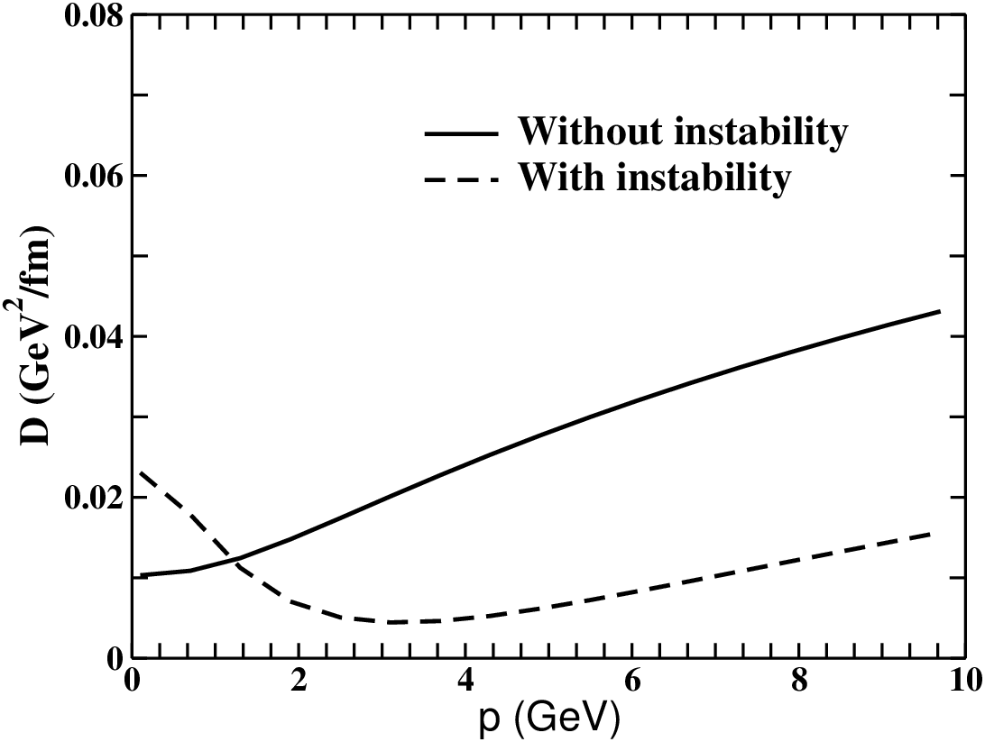
The momentum variation of the drag and diffusion coefficients of charm quark has been depicted in Fig.1 and Fig. 2 with and without instability at RHIC energy by invoking Eq. (III.3.2) in Eq. (2) and Eq.(6) respectively.
The initial temperature () at RHIC energy assumed to be equal to MeV and the corresponding to the temperature MeV is taken as . The initial thermalization time () at RHIC energy is taken as fm. The impact of instability is quite significance (mainly at low momentum range) which decrease the drag coefficient at low momentum, hence, allowing the heavy quarks to move freely . It is worth to mention that the temperature dependence of the drag coefficient play a significance role [18] to describe heavy quark and simultaneously, which is currently a challenge to almost all the models on HQ dynamics. A constant or weak temperature dependence of the drag coefficient is essential to reproduce the heavy quarks and simultaneously. In the presence of instability the drag coefficient decreases at high temperature (at low momentum) and it does not affect the low temperature part of the drag coefficient. Hence, presence of instability alter the temperature as well as the momentum dependence of the drag coefficient and may have a significance role on and relation. We will address these aspects in future works. The variation of the corresponding diffusion coefficient with momentum has been shown in Fig.2 at the RHIC energy with and without instability. In case of diffusion coefficient the impact of instability is noticeable throughout the momentum range considered in this work.



The momentum variation of drag and diffusion coefficients of charm quarks with and without instability at the LHC energy are displayed in Fig.3 and Fig.4 , respectively, showing behavior qualitatively similar to that of the RHIC energy. In case of LHC energy we use MeV and . The initial thermalization time at LHC energy assumed to be fm. At the qualitative front HQ drag and diffusion coefficients both at RHIC and LHC show similar trend at lower as well as higher momentums. This may be due to that fact that the temperature dependence of at RHIC and LHC is not very different.
IV.1 Impact of strength of the anisotropy
To explore the impact of the instability/anisotropy on the heavy-quark dynamics, we vary the parameter from as shown in Fig. 5. As we increase the value of , conversely decreasing the strength of the anisotropy, the heavy quark drag coefficient, at low (less than 4 GeV) increases, in contrast as its behavior at high (larger than 4 GeV). The impact is more pronounced at low momentum. Larger the strength of anisotropy, smaller the , meaning that the anisotropy is creating relatively lesser hindrance for the HQs to travel in the QGP medium, at low momentum, in contrast, to the role played by the anisotropy at high .
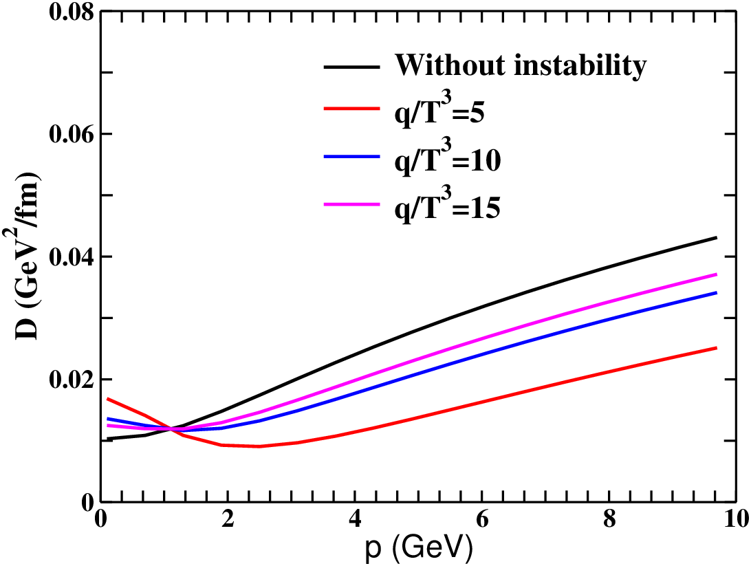
We vary the parameter from as shown in Fig. 6 for the diffusion coefficient. As we increase the value of the heavy quark diffusion coefficient decreases (in low momentum) in contrast to the drag coefficient. The quantity in the figure legends (Figs. 5-8) is defined as: .



V Conclusions and outlook
We have estimated the drag and diffusion coefficients of heavy quarks propagating through a QGP medium considering the role of momentum state anisotropy. The initial momentum anisotropy in the early stages coupled with the rapidly expanding QGP is modeled by setting up an effective transport equation and its solution in near equilibrium approximation leads to the modeling of near(non) equilibrium distribution functions for quark-antiquark and gluons. We have coupled these distribution functions to the kinetic theory description of heavy quark drag and diffusion coefficients and studied their temperature and momentum dependence.
We found that both at RHIC and LHC energies, impact of the anisotropy on heavy quark transport is quite significant as compared to case while HQs are moving in an isotropic QGP medium. The presence of anisotropy alter both the temperature as well as momentum dependences of the heavy quarks drag and diffusion coefficients. These results may have significance impact on and which will be a matter of future investigation. We also intend to explore the impact of bulk viscosity along the similar lines of the analysis.
Acknowledgements
This work has been conducted under the INSPIRE Faculty grant of Dr. Vinod Chandra (Grant no.:IFA-13/PH-55, Department of Science and Technology, Govt. of India) at Indian Institute of Technology Gandhinagar, India. We would like to record our sincere gratitude to the people of India for their generous support for the research in basic sciences in the country. SKD acknowledges the support by the ERC StG under the QGPDyn Grant no. 259684.
References
- [1] Erich S. Weibel, Phys. Rev. Lett. 2, 83 (1959).
- [2] T. Abe and K. Niu, J. Phys. Soc. Jpn. 49, 717 (1980), ibid. 49, 725 (1980); S. Mrowczynski, Phys. Lett. B214, 587 (1988); ibid 314, 118 (1993); P. Romatschke and M. Strickland, Phys. Rev. D 68, 036004 (2003).
- [3] M. Asakawa, S. A. Bass, B. Müller, Phys. Rev. Lett. 96, 252301 (2006); Prog. Theor. Phys. 116, 725 (2007).
- [4] M. G. Mustafa, D. Pal and D. K. Srivastava, Phys. Rev. C 57, 889 (1998)
- [5] G. D. Moore, and D. Teaney, Phys. Rev. C 71, 064904 (2005).
- [6] H. van Hees, V. Greco and R. Rapp, Phys. Rev. C 73, 034913 (2006); Hees, M. Mannarelli, V. Greco and R. Rapp, Phys. Rev. Lett. 100, 192301 (2008).
- [7] P. B. Gossiaux and J. Aichelin, Phys. Rev. C 78, 014904 (2008); P. B. Gossiaux, J. Aichelin, M. Bluhm, T. Gousset, M. Nahrgang, S. Vogel and K. Werner, PoS QNP 2012 (2012) 160.
- [8] Y. Akamatsu, T. Hatsuda and T. Hirano, Phys. Rev. C 79, 054907 (2009).
- [9] S. K Das, J. Alam and P. Mohanty, Phys. Rev. C 82, 014908 (2010); Phys. Rev. C 81, 044912 (2010); S. Majumdar, T. Bhattacharyya, J. Alam and S. K. Das, Phys. Rev. C 84 , 044901 (2012).
- [10] J. Uphoff, O. Fochler, Z. Xu and C. Greiner, Phys. Rev. C 84 024908 (2011); J. Uphoff, O. Fochler, Z. Xu and C. Greiner, Phys. Lett. B 717 (2012) 430
- [11] W. M. Alberico et al., Eur. Phys. J. C, 71 1666 (2011); W. M. Alberico et al., Eur. Phys. J. C 73 2481 (2013)
- [12] Cao S., Qin G.-Y., Bass S A 2013 Phys. Rev. C 88,4, 044907; S. Cao, G. Y. Qin and S. A. Bass, J. Phys. G 40, 085103 (2013).
- [13] S. K. Das, A. Davody Phys. Rev. C 89, 054912 (2014).
- [14] S. K Das, V. Chandra, J. Alam, J. Phys. G 41 015102 (2014).
- [15] Xu H, Dong X, L. Ruan, Q. Wang, Z. Xu, Y. Zhang, Phys. Rev. C 89, 024905 (2014).
- [16] M. He , R. Fries and R. Rapp, Phys. Rev. Lett. 110, 112301 (2013).
- [17] S. K. Das, F Scadina ,S Plumari , V. Greco, Phys. Rev. C 90, 044901 (2014).
- [18] S. K. Das, F .Scardina, S. Plumari and V. Greco, Phys. Lett. B 747, 260 (2015).
- [19] T. Song, H. Berrehrah, D. Cabrera, J. M. Torres-Rincon, L. Tolos, W. Cassing and E. Bratkovskaya, arXiv:1503.03039 [nucl-th].
- [20] S. K. Das, M. Ruggieri, S. Mazumder, V. Greco and J. Alam, arXiv:1501.07521 [nucl-th].
- [21] M. Younus, arXiv:1503.06936 [nucl-th].
- [22] E. M. Lifshitz, and L. P. Pita Pitaevskii, Physics kinetics (Butterworth-Hienemann, Oxford 1981); R. Balescu, Equilibrium and Non-equilibrium Statistical Mechanics (Wiley, New York 1975).
- [23] S. K. Das, J. Alam, and P. Mohanty, Phys. Rev. C 80, 054916 (2009).
- [24] R. Baier, Y. L. Dokshitzer, A. H., Mueller, and D. Schiff, JHEP 0109, 033 (2001).
- [25] S. Jeon, and G. D. Moore, arXiv:hep-ph/0309332.
- [26] M. G. Mustafa, and M. H. Thoma, arXiv:hep-ph/0309332.
- [27] A. K. Dutt-Mazumder, J. Alam, P. Roy and B. Sinha, Phys. Rev. D 71 (2005) 094016; P. Roy, A. K. Dutt-Mazumder and J. Alam, Phys. Rev. C 73 (2006) 044911.
- [28] B. Svetitsky, Phys. Rev. D 37, 2484( 1988).
- [29] M. Cheng et. al, Phys. Rev. D 77, 014511 (2008).
- [30] V. Chandra, V. Ravishankar, Phys. Rev. D 84, 074013 (2011).
- [31] S. Borsanyi et. al, JHEP 1009,073 (2010); JHEP 11, 077 (2010); Y. Aoki et al., JHEP 0601, 089 (2006); JHEP 0906, 088 (2009).
- [32] A. Peshier et. al, Phys. Lett. B 337, 235 (1994), Phys. Rev. D 54, 2399 (1996).
- [33] A. Peshier, B. Kampfer, G. Soff, Phys.Rev. C 61, 045203 (2000); Phys.Rev. D 66, 094003 (2002).
- [34] M. DÉlia, A. Di Giacomo, E. Meggiolaro, Phys. Lett. B 408, 315 (1997); Phys. Rev. D 67, 114504 (2003); P. Castorina, M. Mannarelli, Phys. Rev. C 75, 054901 (2007); Phys. Lett. B 664, 336 (2007);
- [35] A. Dumitru and R. D. Pisarski, Phys. Lett. B 525, 95 (2002); K. Fukushima, Phys. Lett. B 591, 277 (2004); S. K. Ghosh et al., Phys. Rev. D 73, 114007 (2006); H. Abuki, K. Fukushima, Phys. Lett. B 676, 57 (2006); H. M. Tsai, B M ̈ller, J. Phys. G 36, 075101 (2009); M. Ruggieri et. al, Phys. Rev. D 86, 054007 (2012).
- [36] K. Dusling, and T, Schäfer, Phys. Rev. C 77, 034905 (2008); K. Dusling, and D. Teaney, Phys. Rev. C 85, 044909 (2012).
- [37] V. Chandra, Phys. Rev. D 86, 114008 (2012), arXiv:1202:5155 [nucl-th].
- [38] T. H. Dupree, Phys. Fluids 9, 1773 (1966); ibid 11, 2680 (1968).
- [39] V. Chandra and V. Ravishankar, Euro. Phys. J C 59, 705 (2009).
- [40] V. Chandra and V. Ravishankar, Euro. Phys. J C 64, 63 (2009).
- [41] V. Chandra, Phys. Rev. D 84, 094025 (2011).
- [42] A. Majumdar, B. Muller, and X.-N. Wang, Phys. Rev. Lett. 99, 192301 (2007).
- [43] M. Asakawa, S. A. Bass, B. Müller, Nucl. Phys. A854, 76-80 (2011).
- [44] K. M. Burke et al , arXiv:1312.5003v2[nucl-th].
- [45] A. Buzzatti and M. Gyulassy, Phys. Rev. Lett. 108, 022301 (2012.
- [46] X. -F. Chen, T. Hirano, E. Wang, X. -N. Wang and H. Zhang, Phys. Rev. C 84, 034902 (2011) [arXiv:1102.5614 [nucl-th]].
- [47] A. Majumder and C. Shen, Phys. Rev. Lett. 109, 202301 (2012) [arXiv:1103.0809 [hep-ph]].
- [48] B. Schenke, C. Gale and S. Jeon, Phys. Rev. C 80, 054913 (2009) [arXiv:0909.2037 [hep-ph]].
- [49] G. Y. Qin, J. Ruppert, C. Gale, S. Jeon, G. D. Moore and M. G. Mustafa, Phys. Rev. Lett. 100, 072301 (2008) [arXiv:0710.0605 [hep-ph]].