On the Black Hole Mass—X-ray Excess Variance Scaling Relation for Active Galactic Nuclei in the Low-mass Regime

Following Nandra et al. [27] (see also 36, 40, 31), the normalized excess variance is calculated using the definition,

where $N$ is the number of good time bins of an X-ray light curve, $\mu$ the unweighted arithmetic mean of the count rates, $X_{i}$ and $\sigma_{i}$ the count rates and their uncertainties, respectively, in each bin.

As shown by van der Klis [38], van der Klis [39], the excess variance is the integral of the PSD of a light curve over a frequency interval given by Eq. (2),

where $\nu_{\rm min}=\frac{1}{T}$, $\nu_{\rm max}=\frac{1}{2\Delta T}$, $T$ and $\Delta T$ are the time length and the binsize of the light curve, respectively. For a given light curve, it is clear that the exact value of the excess variance is dependent on the length of the light curve (e.g. observational duration) as well as on the binsize $\Delta T$. In order to compare the excess variances of different objects or observations in our sample, the duration (timescale) and the binsize of the light curves should be set to be the same for all the obejects. For this purpose, the light curves are divided into one or more segments of 10 ks in length, and for each of the segment the excess variance is calculated. For observations having more than one segment, the mean of the segments is taken. The results are listed in Table 1.

The uncertainty of the excess variance comes from two sources, one of the measurement uncertainty and the other of the stochastic nature of the variability process, as shown by Vaughan et al. [40]. The measurement uncertainties of the excess variance are estimated following Vaughan et al. [40]:

where $\left<\sigma_{i}^{2}\right>$ is the mean of the square of count rate uncertainties, $F_{var}$ the fractional variability ($F_{\rm var}=\sqrt{\sigma_{\rm rms}^{2}}$), and the other quantities are defined in Eq. (1).

As discussed in Vaughan et al. [40], the light curves of AGN are simply stochastic, meaning that each observed light curve is only one realization of the underlying random variability process, and each realization can exhibit a slightly different mean count rate and variance. The random fluctuations between different realizations lead to non-ignorable scatter in the excess variance. This phenomenon can be reflected in our result: for a source with more than one observation (such as J1023+0405, No. X1 in Table 1), the excess variance varies considerably. The scatter can be significantly reduced if the light curves are sufficiently long, or, equivalently, having a sufficient number of data points. We then compute the uncertainty owing to the stochastic nature of the variability process using the method introduced in Vaughan et al. [40]. We first build a PSD model ⁵⁵ 5 The PSD models used in this paper will be introduced in the next subsection, and all the models yield essentially the same results. to simulate a light curve using the method of Timmer & Koenig [34] with a binsize of 250 s and sufficiently long duration. The light curve is divided into 1000 separate segments of 10 ks. The distribution of the calculated excess variances of all the segments is obtained, from which the range of stochastic uncertainty is found. We take the 68% confidence range for the expected excess variance on each of the timescales to get the stochastic scatter. Thus, from our simulations the scatter due to this random process is $\Delta\log(\sigma_{\rm rms}^{2})=-0.29$ and $+0.24$ for 10 ks light curve of a 250s-binsize.

Finally, the total uncertainties of the excess variance are obtained by combining in quadrature the stochastic and measurement uncertainties, which are at the $68\%$ confidence level. The obtained uncertainties of $\sigma_{\rm rms}^{2}$ are given in Table 1. For an object having more than one observation, the mean and its uncertainty are calculated and used as the final excess variance in the following analysis.

As mentioned above, the excess variance is the integral of the PSD of a light curve over a frequency interval. If the shape of the PSD is known, it is possible to calculate the values of the excess variances, and thus to derive the model relation between the excess variance and black hole mass, which can be compared to observations. For AGN, it has been shown that the PSD function has a standard shape of a broken power-law,

where $\nu_{\rm br}$ is the break frequency [24, 14]. For an AGN with given $M_{\rm BH}$ and $\dot{m}$, $\nu_{\rm br}$ can be determined, though the exact value differs somewhat in different models. From Eq. (2) and (4) the excess variance can be expressed as

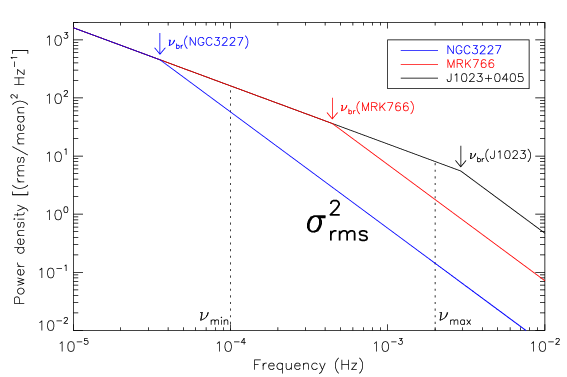
where $C_{1}=A\nu_{\rm br}$ is defined as the PSD amplitude (30, see also model A in 13 for details). It has been suggested that $\nu_{\rm br}$ is inversely scaled with $M_{\rm BH}$, with a possible dependence on the scaled accretion rate in the Eddington units. The relationship between PSD and $\sigma_{\rm rms}^{2}$ is illustrated in the sketch in Figure 3, in which the PSD of three objects in our sample or P12 are shown. The break frequencies derived from $M_{\rm BH}$ and $\dot{m}$ using the González-Martín & Vaughan [14] scaling relation are also indicated for the three objects, which represent the three cases in Eq. (5), respectively.

However, although the broken power-law model given in Eq. (4) is widely accepted, the exact values of the amplitude $C_{1}$ and the break frequency $\nu_{\rm br}$ differ somewhat in different studies. Papadakis [30] first suggested a model with $\nu_{\rm br}=17/(M_{\rm BH}/M_{\odot})$ (Hz) and $C_{1}=A\nu_{\rm br}=0.017$. Later studies with larger samples found a secondary dependence of $\nu_{br}$ on the scaled accretion rate $\dot{m}$ [24, 14], in addition to the dependence on $M_{\rm BH}$. In the literatures of recent studies, three following PSD models of AGN were used:

Model A:

Adopted by González-Martín et al. [13], this model assumes the scaling relation $\nu_{\rm br}=0.003\dot{m}(M_{\rm BH}/10^{6}\ M_{\odot})^{-1}$ suggested by McHardy et al. [24], and a constant PSD amplitude $C_{1}=A\nu_{\rm br}$ ($=0.017\pm 0.006$, 30).

Model B:

The scaling relation for $\nu_{\rm br}$ is the same as in model A. As argued by Ponti et al. [32], the dispersion of the $M_{\rm BH}-\sigma_{\rm rms}^{2}$ relation arising from different $\dot{m}$ derived from model A is too large to account for the observational data, and a new $\dot{m}$ dependent PSD amplitude was suggested: $C_{1}=\alpha\dot{m}^{-\beta}$, where $\alpha=0.003^{+0.002}_{-0.001}$ and $\beta=0.8\pm 0.15$ were fitted in their study.

Model C:

Similar to model A ($C_{1}=0.017$), but an improved scaling relation $\nu_{\rm br}=0.001\dot{m}^{0.24}(M_{\rm BH}/10^{6}\ M_{\odot})^{-1}$ suggested by González-Martín & Vaughan [14], is adopted, which predicts a weaker dependence on $\dot{m}$.

The measured excess variances of 11 low-mass AGN of our sample are calculated from the X-ray light curves obtained in Section 3 using Eq. (1). The results are listed in Table 1. To enlarge the sample, we make use of both the XMM-Newton and ROSAT data, which have somewhat different energy bands. It has been shown that the excess variance is not sensitive to energy bands in the range concerned here [32]. To enlarge the working sample we also include 8 objects ⁶⁶ 6 They are GH18, GH49, GH78, GH112, GH116, GH138, GH142, and GH211. presented in Ludlam et al. [19] which are not in our sample. The excess variance values given in Ludlam et al. [19] are used, which were calculated using a binsize of 200 s, different from ours (250 s). However, the effect of such a difference on the calculated excess variance is negligible ($<2\%$), as found by performing simulations using the method of Timmer & Koenig [34].

Here we study the relation between $\sigma_{\rm rms}^{2}$ and $M_{\rm BH}$ by combining the low-mass sample and the P12 sample. The combined sample has $M_{\rm BH}$ spanning four orders of magnitude, $10^{5}-10^{9}\ M_{\odot}$. The results are shown in Figure 4. Also plotted is the relation [$\log(\sigma_{\rm rms}^{2})=-2.09-1.03\log(M_{\rm BH}/10^{7}M_{\odot})$] derived from the P12 sample only by Ponti et al. [32]. It shows that the $\sigma_{\rm rms}^{2}$ values of the low-mass sample are comparable to the largest values in P12 with higher $M_{\rm BH}$. However, for all the sources in the combined low-mass sample except one, the excess variances fall systematically below the extrapolation of the $M_{\rm BH}-\sigma_{\rm rms}^{2}$ relation derived from the high-mass P12 sample. Our result indicates that, in the low-mass regime, the $M_{\rm BH}-\sigma_{\rm rms}^{2}$ relation may deviate from the previously known linear relation, and is likely to flatten at around $\sim 10^{6}M_{\odot}$ toward the low-mass end. In fact, the low-mass sample objects themselves do not show any correlation between $\sigma_{\rm rms}^{2}$ and $M_{\rm BH}$ (the Spearman’s correlation test gives a null probability of 0.42). To quantify the statistical significance of this deviation, we perform two statistical tests, assuming that the previous inverse linear relation is a good description of the $M_{\rm BH}-\sigma_{\rm rms}^{2}$ relation over the entire mass range. First, we use the two-sided binomial test to find out the probability of having 18 out of 19 low-mass AGN fall below the relation as observed, whereas an equal probability (50%) of falling on either side of the relation is expected. This gives a probability of $7\times 10^{-5}$. Moreover, we fit an inverse linear relation with the slope fixed at -1 in the log-log space to the data of both the low-mass and the P12 sample. The reduced $\chi^{2}/dof$ of the fit is 836/53. Then we assume that the inverse linear relation breaks to a constant at masses below a so-called break mass, which is fitted as a free parameter. The $\chi^{2}/dof$ value for this model is 705/52 (the break mass is fitted to be $1.7\times 10^{6}M_{\odot}$). This improves the fit dramatically by reducing the $\chi^{2}$ by $\Delta\chi^{2}=131$ for one additional free parameter. Despite the fact that although the fitting is statistically not acceptable in terms of the large reduced $\chi^{2}$ (may arise from some intrinsic scatters inherent to the relationship), as an approximation, we employ the F-test [2] to test the significance of adding the flattening term does NOT improve the fit. This yields a small $p$-value 0.003. We thus conclude that the flattening of the inverse linear $M_{\rm BH}-\sigma_{\rm rms}^{2}$ relation toward low-mass AGN is statistically significant. The fitted break mass is $\sim 1.7\times 10^{6}M_{\odot}$.

We also fit a simple linear relation with the slope as a free parameter in the log-log space using the data of both the low-mass and the P12 samples, using the bisector method as in Ponti et al. [32] (see also Appendix A of 4). The best-fit relations are over-plotted in Figure 4 as dotted lines. We find $\log(\sigma_{\rm rms}^{2})=(-2.09\pm 0.044)+(-0.58\pm 0.053)\log(M_{\rm BH}/10^{7}M_{\odot})$. The slope $-0.58\pm 0.053$ deviates significantly from the expected value -1 based on previous studies for AGN samples with higher $M_{\rm BH}$ (e.g. 44, 32).

For low-mass AGN, there appears to be a large scatter in the $\sigma_{\rm rms}^{2}$ values spanning almost one decade. The distribution of the excess variances (in logarithm) for our sample objects with $M_{\rm BH}<2\times 10^{6}M_{\odot}$ is plotted in Figure 5 (left panel), along with a fitted Gaussian distribution (dashed line). It would be interesting to examine the intrinsic dispersion of their $\sigma_{\rm rms}^{2}$ distribution, by taking into account the uncertainty of individual $\sigma_{\rm rms}^{2}$. The maximum-likelihood method as introduced by Maccacaro et al. [20] is used to quantify the intrinsic distribution (assumed to be Gaussian) that is disentangled from the uncertainty of each of the measured excess variance (also assumed to follow a Gaussian distribution). We find a mean $\langle\log(\sigma_{\rm rms}^{2})\rangle=-1.41^{+0.093}_{-0.091}$ with a standard deviation $\sigma=0.22^{+0.088}_{-0.065}$. The confidence contours of the two parameters are shown in Figure 5 (right panel). This indicates that the apparently large scatter of $\sigma_{\rm rms}^{2}$ can mostly be attributed to the uncertainty of each of the measurements (including both the measurement and the stochastic uncertainties), and the intrinsic dispersion is small, but non-negligible (the standard deviation of $\log(\sigma_{\rm rms}^{2})$ $\approx 0.15-0.3$ at the 68% confidence level). It may also suggest that the dependence of $\sigma_{\rm rms}^{2}$ on any other parameters (e.g. accretion rate) is likely not strong.

In conclusion, the previously found inverse scaling of $M_{\rm BH}-\sigma_{\rm rms}^{2}$ for AGN with supermassive black holes cannot be extrapolated to the low-mass regime, but starts to flatten at around $M_{\rm BH}\sim 10^{6}M_{\odot}$. This implies that, although the excess variance can still be used to search for AGN with $M_{\rm BH}\lesssim 10^{6}M_{\odot}$, it fails to provide accurate black hole mass estimation in this mass range. This result is consistent with that obtained in a recent paper by Ludlam et al. [19]. It is also suggested that, for AGN in the $10^{5}-10^{6}\ M_{\odot}$ range, the intrinsic dispersion of the excess variances is likely to be small [standard deviation of $\log(\sigma_{\rm rms}^{2})$ $\approx 0.15-0.3$].

Here we compare the observed $M_{\rm BH}-\sigma_{\rm rms}^{2}$ relation with the predictions based on the above three PSD models. In theory, the $M_{\rm BH}-\sigma_{\rm rms}^{2}$ relation can be deduced from the PSD of AGN using Eq. (5), once the shape and parameters of the PSD model are known. We take the three PSD models in Section 3.2, and fix the $\nu_{\rm br}(M_{\rm BH},\dot{m})$ relation as their original forms. Since the PSD amplitude $C_{1}$ was determined by fitting the $M_{\rm BH}-\sigma_{\rm rms}^{2}$ relation in previous work [30, 32], it is set to be a free parameter here (two parameters $\alpha$ and $\beta$ for model B since $C_{1}=\alpha\dot{m}^{-\beta}$). The bivariate models of $\sigma_{\rm rms}^{2}(M_{\rm BH},\dot{m})$ from Eq. (5) are fitted to the data of both the low-mass and the P12 samples using the simple $\chi^{2}$-minimization fitting. The results are given in Table 2, with the errors of the fitted normalization are at the $68\%$ confidence level. The best-fit PSD amplitudes are very close to their original values for all the models.

The model $M_{\rm BH}-\sigma_{\rm rms}^{2}$ relations using the best-fit PSD normalizations are plotted in Figure 6 for the three models, along with the data. The black, red and blue solid lines represent the relations for three typical accretion rates ($\dot{m}=0.02,0.29,0.97$), respectively, which are the mean (in logarithm) of $\dot{m}$ in three $\dot{m}$ bins (0.01-0.1, 0.1-0.5, and 0.5-4.0). The objects with $\dot{m}$ in the three $\dot{m}$ bins are plotted in corresponding colors. It can be seen that all the three models can reproduce the observed trend of the $M_{\rm BH}-\sigma_{\rm rms}^{2}$ relation well quantitatively. For a given accretion rate, an inverse proportion is predicted in the high $M_{\rm BH}$ regime, whereas in the low-mass regime it flattens toward lower $M_{\rm BH}$. The exact value of $M_{\rm BH}$ at which the relation starts to flatten (the break mass) depends on $\dot{m}$: the higher $\dot{m}$, the larger the break mass. This trend generally holds for all the three PSD models, although the break mass varies from model to model, in addition to its dependence on $\dot{m}$.

Besides this general trend, there are some noticeable differences between the three models. For model A, the strong dependence on $\dot{m}$ leads to a large scatter in high-mass regime over a range of $\dot{m}$. Model B predicts a smaller scatter, but the scatter is relatively larger in the low-mass than in the high-mass regime. Compared to model A, model C also predicts a smaller scatter over the whole $M_{\rm BH}$ range, given its weak dependence of $\nu_{\rm br}$ on $\dot{m}$.

The inverse proportion of the $M_{\rm BH}-\sigma_{\rm rms}^{2}$ relation and its flattening toward low $M_{\rm BH}$ can easily be understood from Eq. (5) and Figure 3. For $\nu_{\rm br}\leq\nu_{\rm min}$ (e.g. NGC 3227 in Figure 3), as $\nu_{\rm br}$ increases (and $M_{\rm BH}$ decreases, since $\nu_{\rm br}\propto{M_{\rm BH}}^{-1}$), the integral of the PSD within [$\nu_{\rm min}$, $\nu_{\rm max}$] increases accordingly, resulting in a linearly increasing $\sigma_{\rm rms}^{2}$. Thus the previously known $M_{\rm BH}-\sigma_{\rm rms}^{2}$ relation (for $M_{\rm BH}>10^{6}M_{\odot}$) is a manifestation of the more fundamental dependence of $\nu_{\rm br}$ on $M_{\rm BH}$ (see also 30, 32). It also shows that the secondary dependence of $\nu_{\rm br}$ on $\dot{m}$ introduces a scatter, the extent of which depends on the models. For $\nu_{\rm min}<\nu_{\rm br}\leq\nu_{\rm max}$ (e.g. MRK 766), the relation becomes non-linear. For $\nu_{\rm br}>\nu_{\rm max}$ (e.g. J1023+0405), $\sigma_{\rm rms}^{2}$ becomes independent of $\nu_{\rm br}$ (thus of $M_{\rm BH}$) and remains a constant.

We have shown that the observed $M_{\rm BH}-\sigma_{\rm rms}^{2}$ relation over almost the whole $M_{\rm BH}$ range for AGN of $M_{\rm BH}=10^{5}-10^{9}\ M_{\odot}$ can be explained qualitatively by the PSD shape of AGN and the dependence of $\nu_{\rm br}$ on $M_{\rm BH}$, although the exact relation depends on the details of the models. It would be interesting to investigate which of the above models give a better description of the data, taking advantage of the extended $M_{\rm BH}$ range provided by our sample. Here we discuss this issue only briefly by comparing the deviations of the data from the models in terms of the fitted $\chi^{2}$, although they are too large for the fits to be acceptable nominally for all the three models (the large $\chi^{2}$ values are partly due to the somewhat large uncertainties in $M_{\rm BH}$ and $\dot{m}$, which are not taken into account in the fitting). We discuss the three models, respectively. (i) Model A has a much larger $\chi^{2}$ value than model B and C, and is likely not a good description of the data. The same suggestion was also argued by Ponti et al. [32]. (ii) For model B, The fitted parameter $\beta$ ($=0.80\pm 0.02$) is consistent with that of Ponti et al. [32]. For the objects with $M_{\rm BH}<2\times 10^{6}\ M_{\odot}$, no correlation is found between $\sigma_{\rm rms}^{2}$ and $\dot{m}$ (the Spearman correlation test gives a null probability $p=0.42$), which seems to be inconsistent to the model prediction (see Figure 6, middle panel). However, this may be partly due to the uncertainties in determining $\dot{m}$. (iii) For model C, our result yields a PSD amplitude consistent with that of Papadakis [30], which is only weakly dependent on $\dot{m}$. This leads the excess variances converging to a constant value toward low $M_{\rm BH}$, which is roughly consistent with the small intrinsic scatter (not zero, however) found above. Overall, based on the fitted $\chi^{2}$ values (Table 2), we tend to consider models B, and perhaps model C to be better descriptions of the PSD shape of AGN. However, a rigorous comparison of the PSD models is beyond the scope of this paper and will be carried out in future work with a larger sample and better quality of data.

References

- [1] Ai, Y. L., Yuan, W., Zhou, H. Y., Wang, T. G., & Zhang, S. H. 2011, ApJ, 727, 31
- [2] Bevington, P. R., & Robinson, D. K. 1992, New York: McGraw-Hill, —c1992, 2nd ed.,
- [3] Bian, W., & Zhao, Y. 2003, MNRAS, 343, 164
- [4] Bianchi, S., Bonilla, N. F., Guainazzi, M., Matt, G., & Ponti, G. 2009, A&A, 501, 915
- [5] Collin, S., & Kawaguchi, T. 2004, A&A, 426, 797
- [6] Dong, X.-B., Ho, L. C., Yuan, W., et al. 2012, ApJ, 755, 167
- [7] Edelson, R., & Nandra, K. 1999, ApJ, 514, 682
- [8] George, I. M., Turner, T. J., Yaqoob, T., et al. 2000, ApJ, 531, 52
- [9] Grandi, P., Tagliaferri,G., Giommi, P., Barr, P., & Palumbo, G. G. C. 1992, ApJS, 82, 93
- [10] Green, A. R., McHardy, I. M., & Lehto, H. J. 1993, MNRAS, 265, 664
- [11] Greene, J. E., & Ho, L. C. 2005, ApJ, 630, 122
- [12] Greene, J. E., & Ho, L. C. 2007, ApJ, 670, 92
- [13] González-Martín, O., Papadakis, I., Reig, P., & Zezas, A. 2011, A&A, 526, A132
- [14] González-Martín, O., & Vaughan, S. 2012, A&A, 544, A80
- [15] Kamizasa, N., Terashima, Y., & Awaki, H. 2012, ApJ, 751, 39
- [16] Kaspi, S., Smith, P. S., Netzer, H., et al. 2000, ApJ, 533, 631
- [17] Lawrence, A., & Papadakis, I. 1993, ApJ, 414, L85
- [18] Lu, Y., & Yu, Q. 2001, MNRAS, 324, 653
- [19] Ludlam, R. M., Cackett, E. M., Gültekin, K., et al. 2015, MNRAS, 447, 2112
- [20] Maccacaro, T., Gioia, I. M., Wolter, A., Zamorani, G., & Stocke, J. T. 1988, ApJ, 326, 680
- [21] Markowitz, A., & Edelson, R. 2001, ApJ, 547, 684
- [22] Markowitz, A., Edelson, R., Vaughan, S., et al. 2003, ApJ, 593, 96
- [23] McHardy, I. 1985, Space Sci. Rev., 40, 559
- [24] McHardy, I. M., Koerding, E., Knigge, C., Uttley, P., & Fender, R. P. 2006, Nature, 444, 730
- [25] Miniutti, G., Ponti, G., Greene, J. E., et al. 2009, MNRAS, 394, 443
- [26] Mushotzky, R. F., Done, C., & Pounds, K. A. 1993, ARA&A, 31, 717
- [27] Nandra, K., George, I. M., Mushotzky, R. F., Turner, T. J., & Yaqoob, T. 1997, ApJ, 476, 70
- [28] O’Neill, P. M., Nandra, K., Papadakis, I. E., & Turner, T. J. 2005, MNRAS, 358, 1405
- [29] Papadakis, I. E., & McHardy, I. M. 1995, MNRAS, 273, 923
- [30] Papadakis, I. E. 2004, MNRAS, 348, 207
- [31] Ponti, G., Cappi, M., Dadina, M., & Malaguti, G. 2004, A&A, 417, 451
- [32] Ponti, G., Papadakis, I., Bianchi, S., et al. 2012, A&A, 542, A83
- [33] Terashima, Y. 2012, Half a Century of X-ray Astronomy, Proceedings of the conference held 17-21 September, 2012 in Mykonos Island, Greece.
- [34] Timmer, J., & Koenig, M. 1995, A&A, 300, 707
- [35] Tremaine, S., Gebhardt, K., Bender, R., et al. 2002, ApJ, 574, 740
- [36] Turner, T. J., George, I. M., Nandra, K., & Turcan, D. 1999, ApJ, 524, 667
- [37] Uttley, P., McHardy, I. M., & Papadakis, I. E. 2002, MNRAS, 332, 231
- [38] van der Klis, M. 1989, Timing Neutron Stars, 27
- [39] van der Klis, M. 1997, Statistical Challenges in Modern Astronomy II, 321
- [40] Vaughan, S., Edelson, R., Warwick, R. S., & Uttley, P. 2003a, MNRAS, 345, 1271
- [41] Vaughan, S., Fabian, A. C., & Nandra, K. 2003b, MNRAS, 339, 1237
- [42] Vestergaard, M., & Peterson, B. M. 2006, ApJ, 641, 689
- [43] Yuan, W., Zhou, H., Dou, L., et al. 2014, ApJ, 782, 55
- [44] Zhou, X.-L., Zhang, S.-N., Wang, D.-X., & Zhu, L. 2010, ApJ, 710, 16
- [45] Zhou, X.-L. 2015, New A, 37, 1
- [46] Zhou, X.-L., Yuan, W., Pan, H.-W., & Liu, Z. 2015, ApJ, 798, LL5