DESY-15-085
Charm, Beauty and Top at HERA
Abstract
Results on open charm and beauty production and on the search for top production in high-energy electron-proton collisions at HERA are reviewed. This includes a discussion of relevant theoretical aspects, a summary of the available measurements and measurement techniques, and their impact on improved understanding of QCD and its parameters, such as parton density functions and charm- and beauty-quark masses. The impact of these results on measurements at the LHC and elsewhere is also addressed.
1 Introduction
HERA was the first and so far only high energy electron11 1 Throughout this document, the term “electron” includes positrons, unless explicitly stated otherwise.-proton collider. The production of heavy-quark final states in deeply inelastic scattering (DIS) and photoproduction () from interactions at HERA (Fig. 1) originally was [1] and still is (this review) one of the main topics of interest of HERA-related physics, and of Quantum Chromodynamics (QCD) in general.


(a) (b)
A quark is defined to be “heavy” if its mass is significantly larger than the QCD scale parameter MeV. The heavy quarks kinematically accessible at HERA are the charm and beauty quarks, which are the main topic of this review. At the time of the proposal of the HERA collider and experiments in the 1980’s [2], a search for the top quark was one of the major goals [3]. This influenced parts of the detector design: if at all, top quarks would be produced boosted into the proton direction, and top-quark mass reconstruction from hadronic final states would profit from an excellent hadronic energy resolution. As we know today, top-quark pair production was out of the kinematic reach of the HERA collider. Single top-quark production is kinematically possible, but strongly suppressed by Standard Model couplings. This allows the search for non-Standard Model top-production processes which will be covered in Section 5.
Charm production at HERA, in particular in deeply inelastic scattering, was realised from very early on to be of particular interest for the understanding of QCD [1, 4]. Up to one third of the HERA cross section is expected to originate from processes with charm quarks in the final state: assuming “democratic” contributions from all quark flavours, which is a reasonable assumption at very high momentum transfers, this fraction can be approximated by the ratio of photon couplings in Fig. 1, which are proportional to the square of the charges of the kinematically accessible quark flavours:
| (1) |
while a similar approximation for beauty yields . In general, the impact of beauty on inclusive cross sections at HERA is thus smaller than the impact of charm.
At momentum transfers large enough for these approximations to be meaningful, charm and beauty can be treated as an integral part of the “quark-antiquark sea” inside the proton (Fig. 2), similar to the light quarks in Fig. 1b, originating from the initial state splitting of virtual gluons. Since the proton has no net charm and beauty flavour number, charm and beauty quarks in the proton can only arise in pairs of quarks and anti-quarks (Fig. 1(a) and shaded part of Fig. 2). However, due to the large charm- and beauty-quark masses of about and , respectively, such a pair is considerably heavier than the mass of the proton. From purely kinematic considerations, it can thus not exist as a “permanent” contribution to the proton in the low-energy limit. Considerations of so-called “intrinsic charm” [5] have been challenging this simple point of view. Since there is no evidence for such a contribution from HERA data [6], this will not be pursued further in this review. Thus, charm and beauty “in the proton”, as depicted in Fig. 2, are always considered to be virtual, and to arise as fluctuations from the perturbative splitting of gluons inside the proton. This establishes heavy quark production as a primary probe of the gluon content of the proton.

Different approaches to the theoretical treatment of charm- and beauty-quark production at HERA are discussed in Section 2. All these treatments crucially make use of the fact that the heavy-quark mass acts as a kinematic cut-off parameter in most of the QCD processes in which heavy quarks occur. Furthermore, the fact that the heavy-quark mass is “large” compared to the QCD scale GeV allows the usage of this mass as a “hard scale” in QCD perturbation theory, appropriately taking into account quark mass effects in perturbative calculations (Fig. 3). On the other hand, the “smallness” in particular of the charm-quark mass with respect to other scales appearing in the perturbative expansion, such as the virtuality of the photon, , or the transverse momentum of a jet or a quark, , can give rise to potentially large logarithmic corrections, e.g. of the form
| (2) |
where is the order of the logarithmic expansion, is the strong coupling constant, and is the heavy-quark mass. The size and treatment of these corrections is one of the issues to be investigated.

During the lifetime of the HERA collider, of order charm and beauty events should have been produced in the H1 and ZEUS detectors, of which have been recorded to tape via both inclusive and dedicated triggers. HERA can thus truly be considered to be a charm factory. Furthermore, the fact that charm- and beauty-quark production at HERA can be studied essentially over its complete kinematic range, from the - or -mass threshold up to squared momentum transfers of order , offers the opportunity to treat HERA as a “QCD laboratory” to test the different possible theoretical approaches to heavy-quark production against experimental data. Many such tests are presented in Sections 6 and 8.
In particular, the charm-production measurements can be used to constrain important QCD parameters, such as the charm-quark mass and its running, and has important consequences for the determination of other parameters like the QCD strong coupling constant, . The measurements can also be used to constrain the charm fragmentation parameters, to constrain the flavour composition of virtual quarks in the proton, and to determine or cross-check the gluon distribution inside the proton. Such measurements and results are discussed in Section 9. Finally, the HERA charm results have a significant impact on measurements and theoretical predictions for many QCD-related processes at hadron colliders, such as the LHC. For instance, the resulting constraints on the flavour composition of quarks in the proton reduce the uncertainties of the LHC - and -production cross sections, and the constraints on the gluon content of the proton are an important ingredient for the determination of the Higgs Yukawa coupling to top quarks from the dominant gluon-gluon-fusion Higgs-production process via an intermediate top quark loop. Such cross-correlations are also discussed in detail in Section 9.
Beauty production at HERA (Sections 7 and 8) offers further complementary insight into the theoretical intricacies of heavy-flavour production in QCD. Due to its higher mass () and a correspondingly smaller value of the strong coupling constant, its perturbative QCD behaviour is somewhat better than the one of charm. However, the beauty mass remains non-negligible over essentially the full accessible phase space of HERA, and a large fraction of the cross section is close to the kinematic -mass threshold. This offers a particularly sensitive handle on the treatment of mass effects in QCD but also requires a particularly careful treatment of these mass effects in order to obtain reliable predictions. Finally, the coupling of the photon to quarks is four times smaller than the coupling to charm quarks (Eq. (1)), and the higher -quark mass yields a strong kinematic suppression. Therefore in practice, depending on the region of phase space probed, the -production cross section at HERA is about orders of magnitude smaller than the cross section for charm production. This makes separation from the background and accumulation of a significant amount of statistics experimentally much more challenging. Also, the experimental analyses of beauty are often not fully separable from those of charm production. One of the highlights is the measurement of the beauty-quark mass (Section 9). Others are the measurement of the total beauty-production cross section at HERA (Section 7), and the potential impact of HERA measurements on -quark-initiated production processes at the LHC (Section 9).
Last but not least, most of the results presented depend on a good understanding of the performance of the HERA machine and the HERA detectors, as well as on mastering the heavy-flavour detection techniques. Unfortunately, only a small fraction of the original data can make it through the various event filtering and reconstruction stages. These aspects will be addressed in Sections 3 and 4.
Except for the shortest ones, each section will start with a brief introduction and close with a summary, such that a reader less interested in the details may decide to skip the reading of the more detailed parts of the section.
Some of the material in this review has been adapted from an earlier unpublished review [7] of one of the authors. Further complementary information, in particular on charmonium and bottomonium production or diffractive charm production, which are not covered by this review, is available elsewhere [8, 9, 10, 11, 12]. The broader context of other physics topics can be explored in a more general review on collider physics at HERA [13].
2 Theory of heavy-flavour production at HERA
This section describes the different theoretical approaches to charm and beauty cross-section predictions, which will be needed later in the discussion of
- •
the Monte-Carlo (MC) based acceptance corrections for the data sets used to obtain cross sections;
- •
the extrapolation of different measurements to a common phase space, such that they can be compared or combined;
- •
the comparison of different theory predictions to the measured cross sections;
- •
the parton-density fits including the heavy-flavour data;
- •
the fits of the charm and beauty masses and their running.
Since there is a large overlap between the theoretical approaches for these different purposes they will be discusssed in a common framework in the following.
2.1 HERA kinematic variables and phase space
The measurements of heavy-quark production at HERA have been restricted, for statistical reasons, to neutral current events (exchange of a neutral boson) and to the kinematic region of the negative four-momentum transfer squared , where photon exchange dominates and exchange can be neglected. Figure 4 illustrates the event kinematic variables for scattering with heavy-quark production via the boson (i.e. photon) gluon fusion process (see also Fig. 1).

The four-momenta of the incoming electron , the outgoing electron and the proton can be used to define the following Lorentz-invariant variables:
| (3) | |||||
| (4) | |||||
| (5) | |||||
| (6) | |||||
| (7) |
Here is the centre-of-mass energy of the system and is the photon virtuality. is the centre-of-mass energy of the system. In the simple Quark Parton Model [14] (QPM) the Bjorken scaling variable describes the proton momentum fraction carried by the scattered parton (Figs. 1(b) and 2). The inelasticity, , gives the fraction of the electron energy taken by the photon in the proton rest frame. Only three of these five kinematic variables are independent. Neglecting the masses of the electron and the proton the following relations between these quantities hold:
| (8) | |||||
| (9) |
In the full QCD case this picture becomes more complicated, as illustrated in Fig. 4, where the proton momentum fraction carried by the gluon does not coincide any longer with Bjorken . However, Eqs. (3) – (9) remain mathematically valid.
The scattering events are classified by the photon virtuality . The regime of small is called photoproduction () and the regime is called Deeply Inelastic Scattering (DIS).
2.2 Perturbative QCD calculations
In fixed-order perturbative QCD (pQCD) the calculation of any parton-level cross section in , , or collisions can be expressed as
| (10) |
where or is one incoming beam particle, and the other, , is a proton. is a “parton” taken from , e.g. the electron or photon itself (DIS and real photons), a slightly virtual photon radiated from the electron (photoproduction), or a gluon or quark from the structure of a real photon or (anti)proton. is a parton taken from the proton, i.e. a gluon or quark. and represent the respective momentum fractions of these partons with respect to their “parent” momenta and . Note that these correspond to Bjorken and as defined in the previous section22 2 and using the improved Weizsäcker-Williams approximation [20] in the case of . only in the case of the quark-parton-model approximation to deeply inelastic scattering, while they have a different meaning in other cases. For example, in Fig. 4, the quantity (rather than ) corresponds to as defined in Eq. (10), while in the photoproduction interpretation, and in the hard DIS interpretation. and are the probability density functions, or parton density functions (PDFs), which give the probability, e.g. in the case, to find a parton of type with momentum fraction in a proton. represents the cross section for the partonic hard scattering reaction. This is sometimes split into the so-called hard process, i.e. the part of the reaction with the highest momentum transfer, and so-called initial state (i.e. occurring before the hard process) or final state (i.e. occurring after the hard process) radiation (Fig. 5). Part of the initial state radiation can also be absorbed into the parton density definition. Three energy scales , and appear in the expansion given by Eq. (10), which is also called factorisation, because the cross section is separated into semi-independent factors.

The renormalisation scale determines the scale at which the value of the strong coupling constant is evaluated, i.e. it is the reference point around which the perturbative Taylor expansion of QCD matrix element (ME) calculations is performed. If the expansion is done to all orders in , the result does not depend on the choice of this scale. After truncation of the series to finite order, the neglected higher-order corrections arising from the contribution of a particular subprocess are minimised if this scale is chosen to be close to the physical scale of the momentum transfer in this subprocess. Since at high enough perturbative order there are always different subprocesses with differing physical scales (see e.g. Figs. 3, 5), no single scale choice can universally cover all such scales. The variation of the cross section with respect to a variation of the renormalisation scale is used to estimate the uncertainty due to the finite-order truncation of this perturbative series. Some further aspects concerning the choice of this scale are discussed in Section 2.11.
The factorisation scale determines at which scale the proton PDFs are evaluated. By default, any initial state radiation (lower blob in Fig. 5) with a momentum transfer smaller than the factorisation scale will be absorbed into the (usually collinear) PDF definition. In contrast, any initial state radiation with a momentum transfer larger than this scale, and all final state radiation down to the fragmentation scale (see Section 2.10), will be considered as part of the matrix element, with correct (noncollinear) kinematics. On one hand, the choice of a lower factorisation scale therefore gives a more detailed description of the initial state radiation kinematics at a given order. On the other hand, the explicit treatment of initial state QCD radiation in the matrix element “uses up” a power of that would otherwise have been available for a real radiation elsewhere in the process, or for a virtual correction. This effectively reduces the order of the calculation with respect to the case where the same radiation is absorbed into the PDF definition, and therefore reduces the overall accuracy of the calculation. Empirically, choosing a factorisation scale equal to or at least similar to the renormalisation scale has been found to be a good compromise.
The third scale, , is conceptually the same as in the , and resolved cases, and therefore taken to be equal to it, while in the electron and direct photon case it is the scale at which the electromagnetic coupling is evaluated for the electromagnetic part of the matrix element (see Section 2.9).
2.3 Heavy-quark production at HERA in “leading order”
In general, the terminology “leading order” (LO), next-to-leading order (NLO), etc. for a perturbative QCD expansion is not unique. It can either refer to a specific power of the strong coupling constant or to a specific number of loops in the perturbative expansion of the matrix elements and/or parton splitting functions contributing to a given process. In order to be precise, this additional information thus needs to be quoted explicitly.
At leading (0-loop) order in QCD, as implemented in the form of tree-level hard matrix elements in most Monte Carlo generators, charm and beauty production in collisions is dominated by boson-gluon fusion (Fig. 6(a)), complemented by other diagrams (Figs. 6(b-d)). Since a or pair is being produced (collectively referred to as ), there is a natural lower cut-off for the mass of the hadronic final state.
In the so-called massless approach (Zero-Mass Variable-Flavour-Number Scheme, ZMVFNS), in which the heavy quark mass is set to 0 for the computation of the matrix elements and kinematics, this natural cut-off is replaced by an artificial cut-off (“flavour threshold”) at for deeply inelastic scattering, or for photoproduction. Below this threshold, which is often applied at the level of the factorisation scale, the heavy-flavour production cross section is (unphysically) assumed to vanish. Above this threshold, heavy quarks are assumed to occur as massless partons in the proton, like the and quarks (Figs. 1(b) and 2). Except for cases in which both final state charm quarks have large transverse momenta , the gluon splitting to in Fig. 6(a) is thus assumed to happen inside the proton, and to be part of the evolution of the parton density functions. The running of is calculated using 3 flavours () below the renormalisation scale , using 4 flavours (including charm) between and , and using 5 flavours above the scale . This results in a quark-parton-model-like scattering of the electron off a heavy quark “in the proton” (Fig. 2), defining the concept of the heavy-quark PDF. In this picture the leading-order process is now an process, while the boson-gluon-fusion graph (Fig. 1(a), with both heavy quarks at high ) is treated as part of the next-to-leading order corrections. This illustrates the partially ambigous meaning of terms like LO, NLO, etc., discussed at the start of this subsection.
Higher order corrections can be applied either by explicitly including them into the calculation of the matrix elements and/or splitting functions, or, if they are to be applied at tree level only, by adding an additional so-called parton shower step. In the latter case, also referred to as leading order plus leading log parton shower (LO+PS), the outgoing and incoming partons of the core “hard” matrix elements are evolved forward or backwards using splitting functions as they are applied during the PDF evolution. Most MCs (e.g. PYTHIA [21], HERWIG [22] and RAPGAP [23]) use the standard DGLAP evolution, as implemented e.g. in JETSET [24] for this purpose. However, in contrast to the PDF evolution, finite transverse momenta are assigned to the partons. Some MCs (e.g. ARIADNE [25]) use a colour dipole model for this evolution, while others use BFKL [26] or CCFM [27] inspired so-called factorisation (e.g. CASCADE [28]). In the context of such MCs, the first diagram in Fig. 6 is referred to as direct production or flavour creation, and the third and fourth are referred to as flavour excitation (in the photon). Either the second only (e.g. PYTHIA) or collectively the last three (e.g. HERWIG) are being referred to as resolved photon processes. The second can uniquely be referred to as a hadron-like resolved-photon process.
For the explicit generation of heavy-flavour final states in such LO+PS MCs, the boson-gluon-fusion diagram (Fig. 1(a)) is optionally treated using massive matrix elements, while for all other diagrams the massless treatment remains the only available option.
2.4 Quark-mass definition
The heavy-quark masses appear in theoretical QCD calculations in several ways. Their physical definition arises from their appearance as parameters in the QCD Lagrangian. The exact value of the masses depends on the renormalisation scheme applied. In the scheme, the masses are defined as perturbative scale-dependent running parameters ( running mass), similar to the running strong coupling constant. In the on-shell mass renormalisation scheme, the masses are defined as the poles of the quark propagator (pole mass), similar to the usual definition of the lepton masses. This is also the definition which one would naively expect to enter phase space calculations. However, since quarks do not exist as free particles, and since the definition of the propagator pole inevitably involves contributions from the nonperturbative region, the pole mass definition has an intrinsic uncertainty of order [29]. At next-to-leading (one loop) order in perturbation theory, the relation between the pole and running mass definitions can be expressed as [30]
| (11) |
where the running mass has been expressed in terms of its value at “its own scale”. Its scale dependence can be expressed as [30]
| (12) |
or alternatively as [31]
| (13) |
with . Higher order expressions can also be found in the quoted references.
At leading (0 loop) order, the difference between the two definitions vanishes. Finally, in the context of so-called massless schemes, the “mass” is defined as a kinematic cutoff parameter in certain parts of the theory calculations.
The pole-mass definition has been used in most QCD calculations relevant for this review. In recent variants of the ABKM [32] and ACOT [33] schemes, the -running-mass definition is used instead. The latter has the advantage of reducing the sensitivity of the cross sections to higher order corrections, and improving the theoretical precision of the mass definition [32].
2.5 The zero-mass variable-flavour-number scheme
In its “NLO” variant, including one-loop virtual corrections (Fig. 7)(b)), the ZMVFNS has been used for most33 3 MRST98 [34] is a notable early exception. NLO variable-flavour parton-density fits up to a few years ago, such as CTEQ6M [35], ZEUS-S [36], H1 [37], NNPDF2.0 [38].


(a) (b) (c) (d)
One of its advantages is that e.g. next-to-leading-log (NLL) resummation of terms proportional to can be applied to all orders, avoiding the problem that such logs could spoil the convergence of the perturbation series at high momentum transfers. However, it is clear that this simplified approach can not give the correct answer for processes near the “flavour threshold”. This has been verified experimentally e.g. for the DIS case [39] (Section 8.2). Also, it was found that neglecting the charm mass in the cross section calculations used for the PDF extraction can result in untolerably large effects on theoretical predictions even at high scales, such as and production at the LHC [40]. All more recent PDF approaches [41, 42, 43, 44, 45, 46, 47] therefore include at least a partial explicit consideration of the charm mass in the matrix elements (Sections 2.6 and 2.7). Nevertheless, since higher orders are more easily calculable in this scheme, the massless approach can offer advantages e.g. in high-energy charm-photoproduction processes [48, 49] in which the consideration of an extra order of in the final state allows a reduction of the theoretical uncertainty (Section 6).
2.6 The massive fixed-flavour-number scheme
The fixed-flavour-number scheme (FFNS) treats the heavy-quark masses explicitly and follows a rigourous quantum field theory ansatz. Full NLO (one loop) calculations of heavy-flavour production in this scheme exist for DIS [50, 51, 52, 53, 54, 55, 46, 47], for photoproduction [56, 57, 58, 59] and for hadroproduction [60]. Some partial NNLO (two-loop) calculations are also available [61, 62]. In this scheme, heavy flavours are treated as massive at all scales, and never appear as an active flavour in the proton. In the case in which all heavy flavours are treated as massive, the number of light flavours in the PDFs is thus fixed to 3, and charm as well as beauty are always produced in the matrix element (Fig. 8). So-called flavour excitation processes (Fig. 6(c,d)), which are often classified as leading order () QCD in partially massless MC approaches [21, 22, 23] of charm or beauty production, appear as NLO corrections in the fully massive approach (Fig. 8).


(a) (b) (c) (d) (e)
There are several variants of the FFNS for heavy-flavour production in DIS (see e.g. remarks in appendix of [63]). In one approach, here called FFNS A, the evolution used together with the 3 flavour PDFs is also restricted to 3 flavours. Thus, the small contribution from heavy flavour loops (Fig. 9(a)) is either treated explicitly in the matrix elements (FFNS A) [46], or, somewhat incorrectly, neglected completely (FFNS A′) [52, 54]. In either variant, this leads to a lower effective value of than in the massless scheme when evolved to high reference scales, e.g. . This is one of the consequences of the non-resummation of terms, and is partially compensated e.g. by a conceptually larger gluon PDF. Despite the conceptual disadvantage of not allowing all order resummation of mass logarithms, this scheme yields very reasonable agreement with charm and beauty data at HERA up to the highest and (Sections 6–8). At HERA energies, the numerical differences between schemes A and A′ are of order 1%, and therefore almost negligible compared to the current data precision.
In the FFNS B approach44 4 Elsewhere [64] this is sometimes called the mixed flavour number scheme. For a discussion see [65][66]. A recent new variant of it [67] is referred to as the “doped” scheme., which was widely used in the early nineties [50, 51, 56, 60, 68], the running of is calculated by incrementing the number of flavours when crossing a flavour threshold, like in the variable-flavour-number scheme. The class of logs corresponding to this running is thus resummed both in the and in the PDF evolution, and the “missing” heavy flavour log resummation is restricted to other cases like gluon splitting and vertex corrections in the matrix elements. This approach is possible since most of the loop and leg corrections which diverge in the massless case, but compensate each other to yield finite contributions, remain separately finite in the massive case. They can thus be separated. At one-loop order, the A and B approaches differ by the way a virtual heavy flavour correction in the BGF matrix element (Fig. 9(a)) (which is missing in the A′ approach) is treated. The FFNS B scheme conceptually yields a value of at high scales which is the same as the one from the variable-flavour approach, and is probably less sensitive to “missing logs” at very high scales than the FFNS A approach. Most NLO photoproduction [56] and hadroproduction [60] calculations, as well as the electroproduction code HVQDIS [51] have been originally designed to be used with the FFNS B scheme.
The A and B approaches both converge to the exact QCD result at infinite order if implemented consistently. The A′ scheme can not converge to the exact result since heavy flavour loop corrections are completely missing, but, as stated earlier, the practical consequences at HERA energies are small. It can however serve as a useful ingredient to variable flavour number scheme calculations (Section 2.7).
There are also other differences. In the ABKM approach, final state gluon splitting (Fig. 9(b,c)) is conceptually treated as part of the light-flavour contribution, while it is treated as part of heavy flavour production in many others [50, 51, 56, 60] (see Section 2.8), as well as in the measured cross sections, since it can hardly be distinguished experimentally. This difference is small [69] in most regions of phase space, but might need to be accounted for when comparing data and theory.
Finally, FFNS calculations in DIS are currently available in leading order (), or NLO () [46, 50, 51]. Partial NNLO (two-loop, ) calculations also exist, based on a full calculation of the and the terms, and the leading term from threshold resummation for the constant term [61]. Further NNLO corrections for the high scale limit [16] have not yet been implemented in practice. Actually, both the NLO and partial NNLO ABKM heavy flavour calculations use the PDFs from their NNLO (two loop, in the matrix elements) fit to the inclusive data [46].
Some of the differences between the calculations discussed in this section and in the next two sections are also summarised in Table 1, using the example of reduced charm cross sections in DIS.
2.7 The general-mass variable-flavour-number scheme
An alternative to the fixed-flavour-number approach is given by the so-called general-mass variable-flavour-number schemes (GMVFNS) [70, 71, 72, 73]. In these schemes, charm production is treated in the FFNS approach in the low- region, where the mass effects are largest, and in the massless approach at very high scales, where the effect of resummation is most noticeable. At intermediate scales (in practice often at all scales above the “flavour threshold”), an interpolation is made between the two schemes, avoiding double-counting of common terms, while making a continous interpolation between differing terms. This scheme combines the advantages of the two previous schemes, while introducing some level of arbitrariness in the treatment of the interpolation.

One of the most constrained schemes is the BMSN scheme [73] used by the VFNS approach of ABKM [62]. At NLO, it interpolates between charm matrix elements in the FFNS part using the ABKM FFNS scheme, and matrix elements in the massless part. It has no tuneable parameters, and (currently) uses the pole-mass definition for the FFNS part. In contrast to most other GMVFNS schemes, the switch to a larger number of flavours should not be made at the “flavour threshold”, but at a scale which is high enough that additional semi-arbitrary kinematic correction terms are not required. In practice, the 3-flavour scheme is used for processes at HERA energies, while the 4- or 5-flavour schemes are recommended for applications at the LHC.
| Theory | Scheme | Ref. | Massive / | Massless | Scale | ||||
|---|---|---|---|---|---|---|---|---|---|
| def. | [GeV] | () | |||||||
| MSTW08 NLO | RT standard | [75] | (pole) | ||||||
| MSTW08 NNLO | approx.- | ||||||||
| MSTW08 NLO (opt.) | RT optimised | [76] | |||||||
| MSTW08 NNLO (opt.) | approx.- | ||||||||
| HERAPDF1.5 NLO | RT standard | [42] | (pole) | ||||||
| NNPDF2.1 FONLL A | FONLL A | [77] | n.a. | ||||||
| NNPDF2.1 FONLL B | FONLL B | (pole) | |||||||
| NNPDF2.1 FONLL C | FONLL C | (pole) | |||||||
| CT10 NLO | S-ACOT- | [55] | n.a. | ||||||
| CT10 NNLO | [78] | (pole) | |||||||
| ABKM09 NLO | FFNS A | [46] | () | - | 0.1135 | ||||
| ABKM09 NNLO | approx.- | - | |||||||
| HVQDIS+ZEUS S | FFNS B | [51] | (pole) | - | 0.118 |
The NLO version of the TR55 5 also referred to as RT scheme [71] combines the charm matrix elements in the FFNS A′ scheme with the matrix elements of the massless scheme, requiring continuity of the physical observables in the threshold region. In this case the usage of the scheme is fully appropriate, since the missing terms will be taken care of by the massless and interpolation terms. Several variants exist for the interpolation, including the so-called standard scheme used e.g. in MSTW08 [43] and HERAPDF1.0 [41], and the optimised scheme preferred for more recent versions, since it avoids a kink in the dependence of the cross section [76]. Both of these variants also exist in a partial NNLO approach [75], including approximate threshold resummation terms for the FFNS part, and a full NNLO calculation for the massless part. They all use the pole mass definition for the FFNS part.
The ACOT [70] scheme, used by CTEQ [44], also exists in several variants. At NLO, (i.e. leading order) FFNS matrix elements are interpolated to (now NLO) massless matrix elements66 6 The fact that similar matrix elements are denoted by different labels concerning their effective order in different context is very confusing, but unavoidable due to different definitions of the truncation of the perturbative QCD series.. Due to the LO FFNS treatment, there is no difference between the pole-mass and running-mass schemes. The interpolation is made in two variants: the S-ACOT approach [79], and the ACOT- approach [80]. The NNLO variant of CT10 [81] uses both FFNS and massless matrix elements at , in the S-ACOT scheme.
The FONLL scheme [69] has 3 variants. The FONLL A approach, used by NNPDF2.1 [45] is equivalent [69] to the CTEQ S-ACOT approach, and uses FFNS heavy-quark matrix elements at NLO. FONLL B and C both use FFNS heavy-quark matrix elements. FONLL B uses matrix elements for light quarks, like MSTW, while FONLL C uses matrix elements for light quarks like ABKM. However, they differ from the latter in the way they treat the interpolation terms. The FONLL C scheme is also similar [69] to the CTEQ S-ACOT NNLO scheme. A full NNLO version of the FONLL A approach also exists [77, 82]. Final state gluon splitting is not included in the charm cross-section predictions for any of these schemes.
The ABM group uses the BSMN approach [73] to generate a GMVFNS scheme out of their FFNS 3-, 4- and 5-flavour PDFs [62].
For photoproduction, a GMVFNS calculation [83] exists for single inclusive cross sections.
All GMVFNS variants use the variable-flavour approach for the running of . Although the mass is unambigously defined in the massive part of the calculation (usually the pole mass), the partial arbitrariness in the treatment of the interpolation terms (Fig. 10) prevents a clean interpretation of the charm and beauty quark masses in terms of a single renormalisation scheme. Therefore, in contrast to the pure FFNS treatment, the charm mass appearing in VFNS schemes can be treated as an effective mass parameter [84]. We will use the symbols and for these effective mass parameters. Alternatively, the presence of the interpolation terms can be included as an additional uncertainty on the respective mass definition [33].
2.8 Proton structure functions in DIS
In analogy to the inclusive neutral current DIS cross section, the cross sections for heavy-quark production in DIS can be expressed in terms of the heavy-quark contributions to the inclusive structure functions [17] , and , denoted by , and ():
| (14) |
where is the electromagnetic coupling constant. The structure function makes the dominant contribution to the neutral current scattering in the kinematic regime accessible at HERA. contains contributions only from interference and exchange, therefore for the region , which was studied at HERA, this contribution is suppressed and can be neglected. The longitudinal heavy-quark structure function parametrises the contribution from coupling to the longitudinally polarised photons. The contribution of to the ep cross section is suppressed for , but can be up to a few percent in the kinematic region of the heavy-quark measurements at HERA and thus can not be neglected.
For both electron and positron beams, neglecting the contribution, the reduced heavy-quark cross section, , is defined as
| (15) |
where . Thus, and only differ by a small correction at high [85].
In the Quark-Parton Model, the structure functions depend on only and can be directly related to the parton density functions. In the QCD case, and in particular for heavy flavour production, this correlation is strongly diluted, and the structure functions depend on both and . More information on the general case can be found e.g. in [17, 41].
Using the example of the charm case [84], the above definition of (also denoted as [69] or [82]) is suited for measurements in which charm is explicitly detected. It differs from what is sometimes used in theoretical calculations in which [69, 75, 86] is defined as the contribution to the inclusive in which the virtual photon couples directly to a or quark. The latter excludes contributions from final state gluon splitting to a pair in events where the photon couples directly to a light quark, and contributions from events in which the photon is replaced by a gluon from a hadron-like resolved photon. As shown in table 1 of [69], the gluon splitting contribution is expected to be small enough to allow a reasonable comparison of the experimental results to theoretical predictions using this definition. The hadron-like resolved photon contribution is expected to be heavily suppressed at high , but might not be completely negligible in the low region. From the point of view of pQCD it appears at and it is neglected in all theoretical DIS calculations used in this review.
2.9 QED corrections
In addition to the different QCD schemes discussed above, predictions of charm production can also differ through their treatment of QED corrections. Some of these corrections, e.g. collinear photon radiation from the initial state electron before the hard interaction (Fig. 11) can actually be large (of order ), and can influence the definition of the , and variables [17]. For photoproduction calculations, the improved Weizsäcker-Williams approximation [20] can be used to parametrise the photon spectrum arising from the incoming electron.

For acceptance corrections (and partially for visible cross sections), predictions including full LO QED radiative corrections, as implemented e.g. in HERACLES [87], are used. For more sophisticated purposes, an NLO version of these corrections is available in the HECTOR package [88]. At the level of the DIS structure functions or it is customary to translate the measured cross sections to so-called Born-level cross sections, i.e. cross sections in which all QED corrections have been removed, to ease comparison of the data with pure QCD predictions. There is one potential exception: the fine structure “constant” can be used in two different ways.
- •
as a genuine atomic scale constant , i.e. all virtual QED corrections are removed, too;
- •
as running in the scheme, i.e. the respective relevant virtual corrections are kept, and a typical value for HERA kinematics is then [89].
The difference between these two approaches in QED has some remote similarity to the difference between the FFNS A and B schemes in perturbative QCD (Section 2.6), treating all quarks and leptons as “heavy” with respect to the atomic scale.
2.10 Fragmentation
Equation (10) allows one to make predictions of heavy-quark production with partons in the final state. However, cross sections are measured and reported mostly in terms of heavy-flavour hadrons, leptons from their decay, or collimated jets of hadrons. Therefore such predictions have to be supplemented with a fragmentation or hadronisation model.
In analogy to collisions [90], the factorised cross section for the production of a heavy-quark hadron as a function of transverse momentum can be written as:
| (16) |
where is the production cross section for heavy quarks (Eq. (10)), is the fragmentation function, is the fragmentation scale and in the fragmentation fraction. The latter is defined as the probability of the given hadron to originate from the heavy quark . The fragmentation function defines the probability for the final-state hadron to carry the fraction of the heavy-quark momentum. The fragmentation function is defined similarly to the PDFs. In the “massless” approximation, it is defined at a starting scale and has to be evolved to a characteristic scale of the process using perturbative QCD. In the massive fixed flavour approach, this evolution can be conceptually absorbed into the pole mass definition.
Fragmentation fractions as well as the starting parametrisation of the fragmentation function can not be calculated perturbatively. Thus they have to be extracted from data. Comprehensive phenomenological analyses of the charm and beauty fragmentation functions in collisions have been performed [91, 92, 93]. While the QCD evolution is process-dependent, the non-perturbative ingredients of the fragmentation model are assumed to be universal77 7 The non-perturbative fragmentation function is universal only if it is accompanied by appropriate evolution.. Comparing measurements from HERA and results from colliders one can test this universality.
However, the tools that are available for fixed-order calculations of the heavy-quark production cross sections in collisions, which are mostly used for exclusive final states, do not comprise a perturbative component of the fragmentation function. Therefore, an “independent” non-perturbative fragmentation function is used in conjunction with the parton-level cross sections. The parametric forms of the independent fragmentation functions most commonly used at HERA are due to Peterson [94]:
Kartvelishvili [95]:
and to the Bowler modification of the symmetric Lund [96] parametrisation:
where , , , and are free parameters that depend on the heavy-flavour hadron species and have to be extracted from data. Since no QCD evolution is applied, the corresponding parameters might be scale- and process-dependent.
2.11 Choice of renormalisation scale
For many cross-section predictions the dominant contribution to the theoretical uncertainty arises from the variation of the renormalisation and factorisation scales by a factor 2 around some suitably chosen default scale. Such a variation is intended to reflect the uncertainty due to uncalculated higher orders. It might therefore be useful to consider some phenomenological aspects of these scale choices as considered in a mini-review on beauty production at HERA and elsewhere [97], focusing in particular on the choice of the renormalisation scale.
Ideally, in a QCD calculation to all orders, the result of the perturbative expansion does not depend on the choice of this scale. In practice, a dependence arises from the truncation of the perturbative series. Since this is an artefact of the truncation, rather than a physical effect, the optimal scale can not be “measured” from the data. Thus, it must be obtained phenomenologically.
Traditionally, there have been several options to choose the “optimal” scale, e.g.
- •
The “natural” scale of the process. This is usually taken to be the transverse energy, , of the jet for jet measurements, the mass, , of a heavy particle for the total production cross section of this particle, or the combination for differential cross sections of such a particle. Often, this is the only option considered. The choice of this natural scale is based on common sense, and on the hope that this will minimise the occurrance of large logs of the kind described above, for the central hard process. However, higher order subprocesses such as additional gluon radiation often occur at significantly smaller scales, such that this choice might not always be optimal.
- •
The principle of fastest apparent convergence (FAC) [98]. The only way to reliably evaluate uncalculated higher orders is to actually do the higher-order calculation. Unfortunately, this is often not possible. Instead, one could hope that a scale choice which makes the leading-order prediction identical to the next-to-leading-order one would also minimise the NNLO corrections. This principle, which can be found in many QCD textbooks, can not be proven. However, recent actual NNLO calculations might indicate that it works phenomenologically after all (see below).
- •
The principle of minimal sensitivity (PMS) [99]. The idea is that when the derivative of the cross section with respect to the NLO scale variation vanishes, the NNLO corrections will presumably also be small. Again, there is no proof that this textbook principle should work, but actual NNLO calculations might indicate that it does (see below).
To illustrate these principles, consider two examples. First, the prediction for the total cross section for beauty production at HERA-B [100] (Fig. 12). The natural scale for this case is the -quark mass, , and all scales are expressed as a fraction of this reference scale. Inspecting Fig. 12, one finds that both the PMS and FAC principles, applied to the NLO prediction and to the comparison with LO (NLO stability), would yield an optimal scale of about half the natural scale. The same conclusion would be obtained by using the NLO+NLL prediction, including resummation, and comparing it to either the LO or the NLO prediction (NLO+NLL stability).


Second, the prediction for Higgs production at the LHC [101] (Fig. 12). The reference scale is now the Higgs mass (). However, inspecting the behaviour of the LO and NLO predictions, neither the FAC nor the PMS principle would yield a useful result in this case, since the two predictions do not cross, and the NLO prediction does not have a maximaum or minimum. This situation occurs rather frequently, and is also true for production at HERA. Fortunately, in the case of Higgs production, the NNLO and even approximate NNNLO predictions have actually been calculated (Fig 12). Applying the FAC and PMS prescriptions to these instead (NNLO stability), again a scale significantly lower than the default scale would be favoured. This might indicate that choosing a scale which is smaller than the default one makes sense even if the FAC and PMS principles do not yield useful values at NLO.
Beyond these examples, a more general study is needed to phenomenologically validate this approach. To avoid additional complications arising from a multiple-scale problem caused by e.g. the scale at HERA or the scale at LEP, the study was limited to cross sections for photoproduction at HERA, or hadroproduction at fixed-target energies, the Tevatron, and LHC. The somewhat arbitrary selection of processes includes beauty production at the [102, 103], the Tevatron [103], and HERA-B [100], top production at the Tevatron [100, 103], direct photon production at fixed target [104], [105] and Higgs [101] production at the LHC, jets at HERA [106] and at the Tevatron [107]. This selection is obviously not complete, and many further calculations, in particular NNLO calculations, have been achieved since this study [97] was originally made. However, it is not biased in the sense that all processes that were originally considered were included, and none were discarded. Clearly, a quantitative update of this study would be useful, but was not yet done. Qualitatively, all newer predictions which the authors have been made aware of either confirm this conclusion, or at least do not significantly contradict it.

In each case the natural scale as defined above was used as a reference. In addition, wherever possible, the optimal scales from both the FAC and PMS principles, evaluated at NLO (NLO stability), NLO+NLL (NLO+NLL stability), and/or NNLO/NNNLO (NNLO stability) were evaluated separately. Figure 13 shows the result of this evaluation. Each crossing point, maximum, or minimum in Fig. 12 yields one entry into this figure, and similarly for all the other processes. The conclusion is that the FAC and PMS principles tend to favour scales which are around 25-60% of the natural scale. Amazingly, this seems to be independent of whether these principles are applied at NLO, NLO+NLL, or NNLO level. For the jet [107] or b-jet [108] cross sections at the Tevatron, it has in part already become customary to use half the natural scale as the central scale.
Using the natural scale as the default and varying it by a factor two, which is the choice adopted for most data/theory comparisons, covers only about half the entries, while the other half lies entirely below this range. Instead, using half the natural scale as the default and varying it by a factor two, thus still including the natural scale in the variation, covers about 95% of all the entries.
This yields the following conclusions.
- •
Obviously, whenever an NNLO calculation is available, it should be used.
- •
Whenever possible, a dedicated scale study should be made for each process for the kinematic range in question. Although there is no proof that the FAC and PMS principles should work, in practice they seem to give self-consistent and almost universal answers for processes at fixed target energies, HERA, the Tevatron, and the LHC.
- •
In the absence of either of the above, the default scale should be chosen to be half the natural scale, rather than the natural scale, in particular before claiming a discrepancy between data and theory. Empirically, this should enhance the chance that the NNLO calculation, when it becomes available, will actually lie within the quoted error band. To evaluate uncertainties, the customary variation of the central scale by a factor 2 up and down remains unaffected by this choice.
The latter principle has already been applied to a few of the results covered in this review. Of course, choosing the natural scale as the central value, which is still the default for most calculations (or making any other reasonable scale choice), is perfectly legitimate and should also describe the data within the theoretical uncertainties. However, if it does not, it might be useful to consider alternative choices as discussed above before claiming evidence for the failure of QCD, and hence for new physics.
Further complementary information, in particular on the related theory aspects, is available elsewhere [109].
2.12 Summary
The theory of heavy flavour production in the framework of perturbative QCD, and in particular the occurrence of different possibilities to treat the heavy quark masses in the PDF, matrix element and fragmentation parts of the calculation, introduces a significant level of complexity into the corresponding QCD calculations, in addition to the usual scheme and scale choices. Confronting different choices with data can be helpful to understand the effects of different ways to truncate the perturbative series.
The majority of the available MC calculations for the analysis of HERA data is based on leading order (plus parton shower) approaches, combining a massive approach for the core boson-gluon fusion process, and the massless approach for tree level higher order corrections. It will be demonstrated in the later chapters that this is fully adequate for acceptance corrections. For comparisons of the measured differential cross sections with QCD predictions, a next-to-leading order massive approach (fixed flavour scheme) is the state of the art.
In some cases massless calculations are still in use, e.g. to facilitate the perturbative treatment of fragmentation, or to implement resummation of some of the logarithms arising when the mass competes with other hard scales occurring in a process. In particular for the prediction of the inclusive heavy flavour structure functions in DIS, a variety of so-called general-mass variable-flavour schemes are available, merging massive calculations at low scales with massless calculations at high scales. These are particularly useful for the extraction of PDFs over very large ranges in energy scale. Partial NNLO calculations are also available for such inclusive quantities, both in the fixed and variable flavour number schemes. Due to the absence of extra semi-arbitrary parameters, the fixed flavour number scheme is particularly well suited for the extraction of QCD parameters like the heavy quark masses.
In general, QED corrections are nonnegligible, and available both at leading and next-to-leading order. Since is much smaller than , the leading order precision is often sufficient. Several competing fragmentation models are in use, and the perturbative treatment of fragmentation in the massive approach is still in its infancy.
Since higher order corrections are large, the uncertainties reflected by the QCD scale variations are often dominant. Until full NNLO calculations become available, a careful consideration of the choice of these scales can be helpful to avoid premature conclusions concerning potential discrepancies between the theory predictions and the data.
3 The HERA collider and experiments
In this section, the HERA collider, the H1 and ZEUS experiments, as well as the reconstruction of the data from these experiments will be briefly described, with focus on aspects relevant for heavy flavour production.
3.1 HERA
HERA (German: Hadron-Elektron-Ring-Anlage) was the first and so far the only electron–proton collider. It was located at DESY in Hamburg, Germany. The circumference of the HERA ring (see Fig. 14) was . The accelerator was in operation from 1992 to 2007.

Electrons or positrons and protons were accelerated in two separate rings to final energies of and ( before 1998), respectively, leading to a centre-of-mass energy of ( before 1998). Both beams were stored in 180 bunches. The bunch-crossing rate was . Electrons and protons collided in two interaction regions, where the H1 and ZEUS detectors were located.
In the years the HERA collider was upgraded to increase the instantaneous luminosity. At the same time a number of upgrades of the H1 and ZEUS detectors were put in place, as described below. Therefore, the data taking was subdivided into two phases: “HERA I” and “HERA II” corresponding to the data taking periods and , respectively. In 2007, a few months were dedicated to data taking at lower centre-of-mass energies.
3.2 H1 and ZEUS Detectors


The H1 and ZEUS detectors were typical modern multi-purpose collider experiments and are described in detail in [110, 111, 112, 113]. Figure 15 visualises the layout of the H1 and ZEUS detectors88 8 The right-handed Cartesian coordinate system used at H1 and ZEUS has the axis pointing in the nominal proton beam direction, referred to as the “forward direction”, and the axis pointing towards the centre of HERA. Its coordinate origin is at the nominal center of the respective detector, which coincided with the nominal interaction point in the HERA I period. The pseudorapidity is defined as , where the polar angle, , is measured with respect to the proton beam direction. The -- or --plane is also denoted as the transverse plane. . Due to significantly higher energy of the protons there was more detector hardware installed in the direction of the outgoing proton beam. The figures show the key parts of the main detectors that were used for tagging and reconstruction of heavy-flavour events. Some of the most important benchmarks of the H1 and ZEUS detectors, such as polar angle coverage and momentum, the energy resolution and the resolution of the impact parameter 99 9 Also referred to as the transverse distance of closest approach to the nominal vertex, are listed in Table 2.
| H1 | ZEUS | |
| Silicon vertex detector: | CST | MVD |
| # layers | 2 | |
| -coverage | ||
| -coverage | ||
| Drift chambers: | CTD | CTD |
| -coverage | ||
| -coverage | ||
| Calorimeters: | LAr | CAL (HERA I) |
| -coverage | ||
| -coverage | ||
| El.-magn. | ||
| Hadronic | ||
| SpaCal | ||
| -coverage | ||
| -coverage | ||
| El.-magn. | ||
| Muon systems: | CMD | R/B/FMUON+BAC |
| -coverage | ||
| -coverage |
In the following the main components of the H1 and ZEUS detectors are discussed with emphasis on the advantages of the respective designs:
Tracking Chambers:
Tracks from charged particles were reconstructed based on the position measurements in the large Central Drift Chambers. The pulse height on the sense wires was used to measure the energy loss in the detector medium, . The measurements were used for particle identification, distinguishing between electrons, pions, kaons and protons in a limited momentum range. The important differences between H1 and ZEUS are:
- •
- •
For ZEUS a superconducting coil surrounded the tracking detectors and provides a magnetic field of 1.43 Tesla. This is considerably higher than the 1.15 Tesla delivered by the H1 superconducting coil, situated outside the calorimeter. In both experiments the magnetic field within the tracking system was parallel to the axis.
- •
Four of the nine superlayers of the ZEUS chambers were equipped with stereo wires, which were tilted with respect to the beam axis. This provided -measurement points for tracks with a resolution of . At H1 the sense wires were strung parallel to the beam axis and the track -position measurement was obtained by the division of the charges recorded at both wire ends, yielding a moderate resolution of a few centimetres. Two additional -drift-chambers were installed to provide for each track a few -measurement points with typically resolution.
In the forward region H1 and ZEUS have installed a Forward Tracking Detector (FTD) [115] and a Straw Tube Tracker (STT) [116], respectively, that are based on drift-chambers. Their main purpose is to extend the polar angular coverage to angles smaller than , outside the acceptance of the central drift chambers. However, for both experiments these detectors have not been used for momentum reconstruction due to a large amount of dead material in front of them. Nevertheless, the forward detectors were partially used in the pattern recognition.
Vertex-detector:
The Central Silicon Tracker (CST) [117] and the Micro Vertex Detector (MVD) [118] were located in the heart of the H1 and ZEUS experiments. The MVD was installed only for the HERA II data taking. The vertex detectors allowed the determination of trajectories of charged particles in the vicinity of the primary vertex. The achieved precision was sufficient to resolve vertices from secondary decays. This is essential for the tagging of weakly-decaying heavy-flavour hadrons with a typical lifetime .
The CST (MVD) consisted of two (three) () long concentric cylindrical layers of double-sided silicon-strip detectors The innermost layer of the CST and MVD was located at and , respectively. The most important benchmarking parameters are given in Table 2. The following intrinsic hit resolutions were achieved: for the CST and for the MVD. The CST had a somewhat better average transverse impact parameter resolution mainly due to less material, hence less multiple scattering, but was essentially restricted to track reconstruction in the transverse plane. The MVD contained four wheels of double-sided silicon-strip detectors in the forward region that extended the polar-angle coverage from to . Furthermore, it allowed 3D standalone pattern recognition. At H1 the CST was supplemented with the forward and backward strip detectors, FST and BST, that extended the polar-angle coverage of CST to . However, these were not used in H1 heavy-flavour analyses.
Calorimeters:
The tracking detectors were surrounded by calorimeter systems, which covered almost the full solid angle. Their main tasks were to identify and measure the scattered electron, to reconstruct the hadronic final state (e.g. jets) and photons and to separate electrons from hadrons. At H1 a fine-grain liquid-argon (LAr) sandwich calorimeter [111, 119] was installed in the central and forward region. It was supplemented in the backward region with the lead-scintillating fibre calorimeter SpaCal [112, 120]. In the ZEUS detector the solenoid was surrounded by a high-resolution compensating uranium–scintillator calorimeter (CAL) [121]. The calorimeters had inner electromagnetic and outer hadronic sections. The electron and hadron energy scales of the calorimeters were known at the level of and , respectively. The calorimeters were calibrated from the data using kinematic constraints. Overall, both calorimeter systems performed very well.
Additionally, for detection of very-low- events, where the electron is scattered at a small angle, ZEUS installed the beampipe calorimeter (BPC) [122]. This calorimeter was in operation in HERA I and was located just from the beam line. It allowed the extension of the phase-space coverage to
Electron taggers:
Both H1 and ZEUS were equipped with special detectors, called electron taggers, which were able to detect electrons scattered at very small angles. Especially during the HERA I period, these could be used to explicitly identify photoproduction events in specific ranges of .
Muon systems:
To identify muons both experiments installed large arrays of limited-streamer tubes [111, 123] inside and outside the magnetic return yoke (not shown), which covered a wide range in polar angle and measured muons efficiently for transverse momenta above , with significant partial acceptance also at lower . The return yoke of the ZEUS detector was also equipped with drift tubes providing complementary muon identification and serving as a backing calorimeter (BAC). A forward muon system completed the coverage of the tracking detectors. The H1 detector had a similar muon coverage, including the usage of the liquid argon calorimeter as a tracking calorimeter.
Luminosity measurement:
In both experiments the luminosity was measured using the photon bremsstrahlung process . The photons were detected by dedicated detectors [124, 125] about away from the interaction points in the -beam direction. In addition, H1 also used the SpaCal to measure the large-angle QED compton scattering [126]. The ultimate precision of the luminosity measurement by H1 (ZEUS) is () for the HERA II period and () for the HERA I period.
Trigger and readout system:
Both H1 [127] and ZEUS [113, 128] have used a multi-level trigger system to select interesting events online and to suppress background from beam–gas interactions. The H1 trigger system consisted of two hardware layers and one software filter. It was supplemented for the HERA II period by an additional track trigger. The ZEUS trigger was based on one hardware and two software levels. The first two levels mostly operated with the energy sums in the calorimeter, timing and limited tracking information. On the third level a complete reconstruction of the event is performed, using a simplified version of the offline reconstruction software, to select more sophisticated objects like jets, tracks and even D-meson candidates. The triggers reduced the rate from the nominal HERA bunch-crossing rate to the storage rate . While the topology of DIS events allowed triggering on the scattered electron inclusively already at the first level of the trigger chain, triggering on heavy-flavour photoproduction was more challenging and required reconstruction of leptons, tracks, hadronic activity in the calorimeter or even explicitly charm hadrons. Both experiments had capabilities to include limited tracking information already at the first trigger level, for instance on the number of tracks and the fraction which originates from the interaction vertex.
3.3 Event reconstruction
Various heavy-flavour tagging techniques (see Section 4) exploit different measured quantities, like tracks, vertices, energy-flow objects, jets and muons. The reconstruction of these quantities is described in the following:
Tracking:
Tracks were reconstructed combining hits from the central tracking chambers, silicon-strip detectors and forward/backward trackers for high . In both experiments tracks were parametrised with a helix defined by 5 parameters (Fig. 16 shows the --view): the curvature , which is the signed inverse radius, , the dca distance of closest approach in the plane, , the azimuth angle, , the distance of closest approach along the axis, and the polar angle .

To account for multiple scattering and energy loss in the material along the track trajectory and for inhomogeneities of the magnetic field, the track parametrisation was refined in a track-refit process based on a broken-lines algorithm [129] in H1 and a Kalman filter [130] in ZEUS. Additionally, the parameterisation of all tracks that were fitted to the primary or to a secondary vertex (see below) was further improved by a track refit using the vertex position as a constraint.
Analyses that aimed at the best tracking precision used tracks with typically . This coverage corresponds to the region where efficiencies and resolutions are high and well known. Performance benchmarking for the two tracking systems is shown in Table 2.
At low momenta, the measurement for each track allowed the separation of pions, kaons and protons, while at high momenta electron/hadron separation was possible to some degree.
Vertexing:
Reconstructed tracks were used as an input for the primary vertex in each event. In addition, if silicon-strip information was available, the time-averaged mean position of the interaction region, the beam spot, was used to further confine the position of the primary vertex in the event. The beam spot was measured by the experiments as a function of time for each events. The beam spot size in the transverse plane was measured to be and in H1 HERA I data, and in H1 HERA II data, and and in ZEUS HERA II data. The beam-spot size along the axis was much larger, , and therefore was not used as a constraint. In H1 the vertex fitting was performed in the plane1010 10 An iterative procedure to determine the position of the primary vertex was used., while ZEUS did a full vertex fit in . Nevertheless, both experiments used only the projections of decays in heavy-flavour analyses due to superior resolution.
In addition, in the context of some ZEUS heavy-flavour analyses, selected tracks were removed from the primary vertex fit and the fit was re-done. Combinations of such tracks were fitted to a displaced secondary vertex that was associated with a decay of a heavy-flavour hadron. Procedures similar to those used in the primary-vertex fit1111 11 For obvious reasons, no beamspot constraint is used. are used to fit the secondary vertices as well. Alternatively, combinations of impact parameters of several tracks were used in H1. Secondary vertices give an important handle:
- •
to test the hypothesis that selected tracks originate from a decay of the same particle by evaluation of the of the secondary vertex;
- •
to evaluate the flight distance of that particle, which is related to the particle .
This will play an essential role (together with the track impact parameter) in the heavy-flavour lifetime tagging (cf. Section 4).
Electron reconstruction:
Electron identification was needed to reconstruct DIS events as well as to measure semi-leptonic decays of beauty and charm quarks. Electrons were separated from hadrons using the shape of clusters in the calorimeter and information from the central drift chambers. A typical phase-space coverage for electrons in a beauty-production measurement in the semi-leptonic electron decay channel was () and () for the H1 (ZEUS) measurements.
Muon reconstruction:
Muons were identified by combining information from the tracking systems, calorimeters and muon chambers. For ( GeV) the information from the muon chambers was exploited and the fraction of hadrons which were misidentified as muons was typically less than . For momenta isolated muons can be efficiently identified in the calorimeters, using “minimum ionising particle” (mip) signatures, which however leads to reduced purity. The efficiency to identify high momentum isolated muons in the H1 and ZEUS muon systems was and [131], respectively.
The wide coverage of the muon chambers allowed the extension of the phase space of the measurements up to .
Hadronic system:
Energy flow objects (EFOs) were used in both experiments to reconstruct the hadronic final state [132, 133]. These objects were based on a combination of information from the calorimeter and the tracking system optimising energy resolution. Track information is superior for low-energy EFOs, while the calorimeter measurement is preferred at high energy as well as to measure neutral particles.
Jets at HERA have been reconstructed with the inclusive clustering algorithm [134, 135]1212 12 Mostly in the longitudinally-invariant mode with the massless and massive recombination schemes [136] in the H1 and ZEUS experiments, respectively. The parameter was set to , which is larger than the values used typically at and experiments (), since at HERA jets with relatively low transverse momenta were analysed. The chosen jet algorithm is infrared and collinear safe to all orders in perturbation theory. It was checked [137] that at HERA the , anti- [138] and SIScone [139] algorithms produce very similar measurement results and that the precision of NLO QCD calculations for the anti- algorithm is very similar to that of the algorithm.
The final precision of the jet energy scale uncertainty of the H1 and ZEUS calorimeters was (see [140] for a recent review of jet results from HERA).
3.4 Summary
HERA was the first and so far only high energy collider. The results discussed in this review were obtained with the H1 and ZEUS detector in two different running periods, denoted “HERA I” and “HERA II”. The main detector parts relevant for the detection and reconstruction of heavy flavour events were the electromagnetic part of the calorimeters for the reconstruction of the scattered electron (if detectable), the calorimeters and tracking systems for the reconstruction of the decay products of heavy flavoured particles, and the muon systems for the detection of semileptonic decay final states.
4 Charm and Beauty detection at HERA
The large charm- and beauty-quark masses result in kinematical suppression of their production compared to the light-flavour cross sections. Therefore, special techniques have to be employed to separate charm and beauty “signal” from the dominating light-flavour “background”. These techniques utilise distinct properties of the charm and beauty hadrons (see Fig. 17 for illustration):

- 1.
Flavour tagging. The tagging of the quark flavour is done either by full reconstruction of decays of heavy-flavoured hadrons or by lepton tagging from the semi-leptonic decays of those hadrons. The former was used at HERA only for charm tagging, since low production rates and small branching ratios for useful decays led to insufficient statistics for fully-reconstructed beauty hadrons. The latter was mostly used for beauty tagging, since -hadron decays produce leptons with sufficiently high momenta for efficient identification in the detectors.
- 2.
Lifetime tagging. This method exploits the relatively long lifetimes of weakly-decaying heavy-flavour hadrons through the reconstruction of tracks with large impact parameter or displaced secondary vertices. In addition, the information about the flight direction, extracted from either the track, hadron or jet momentum, can be used to construct a signed impact parameter or a signed decay length (see later). This is a powerful tool to separate charm and beauty from light-flavour events, in which tracks mostly originate from the primary vertex.
- 3.
Mass tagging. The tagging using the mass of the heavy quark or meson is performed either explicitly by a full reconstruction of the mass from all decay products (also see flavour tagging), by a partial reconstruction via the mass of a jet or of all tracks at a secondary vertex, or indirectly by measuring the relative transverse momentum of a particle with respect to the axis of the associated jet, . The latter was mostly used to separate beauty events from production of other flavours, since the large quark mass produces large values.
The above methods are all based on measuring the decay particles of one heavy quark (single tag). Several methods can be combined to increase the purity at the cost of statistics. Both heavy quarks (double tag) in an event can be tagged, by applying one method to tag one heavy quark and another (or the same) for the other heavy quark. This allows a more detailed study of the heavy-quark production mechanisms, but the double tagging efficiencies are low.
In the following the different tagging methods are discussed in more detail with emphasis on the advantages and disadvantages of each method.
4.1 Charm tagging using full reconstruction of charm hadrons.
Most of the HERA charm results have been made using the golden decay channel (see Fig. 18)1313 13 Throughout the paper the is mostly referred to as . The full reconstruction of ’s at HERA was impossible since the resulting decay photon or could not be reliably measured..


Occasionally, also the decay channel was used to increase statistics. Due to the small energy release in the decay () the phase space for combinatorial background is suppressed, and the resolution for the mass difference is strongly enhanced, providing an excellent signal to background ratio. This also leads to a small momentum of the produced pion, which is often called the “slow” pion, . The capability of a detector to measure very-low-momentum tracks defines the accessible region of and therefore the phase space of the : a typical restriction leads to . For some analyses the cut was raised to suppress the combinatorial background, which rises at low (cf. Fig. 18 (a) and (b)). For the signal extraction, the observable was chosen. The number of signal events is determined either by counting the number of events in the peak region after subtracting the combinatorial background, which is estimated from the distribution of “wrong charge” combinations, by fitting the spectrum with a Gaussian-like shape for the signal and a phenomenological function for the background, or by a combination of these two methods.
Besides the golden decay channel, the , , and decays of charm hadrons were used to tag charm in the events. These charm hadrons feature much larger background (see Fig. 18(c) for an example of a measurement). However, a lifetime tag can be added, exploiting the relatively large values for the weakly-decaying charm hadrons. The decay length is reconstructed by fitting a displaced secondary vertex to selected tracks of decay products (see Section 4.3 for more details). This combined approach allowed to significantly reduce combinatorial background, most noticeably for the that has the largest lifetime (cf. Fig. 18(c) and (d)), to a level that is still somewhat worse than but comparable to the . Nevertheless, due to the low boost, lifetime tagging is inefficient in the phase space that is also not accessible with ’s. In this region it is beneficial to study particular decay channels with neutral strange hadrons or , for example .
The H1 and ZEUS experiments achieved a similarly good signal mass-peak resolution for charm hadrons. Note that the distributions in Fig. 18 can not be compared directly due to different kinematic regions.
In summary, the advantages () and disadvantages () of full hadron reconstruction are:
-
The full reconstruction allows an accurate determination of the momentum of the charm hadron, which is correlated with the kinematics of the charm quark and can be used to study the fragmentation process.
-
An excellent signal to background ratio of can be achieved using the golden decay channel or the reconstruction of other weakly-decaying mesons including a lifetime tag (Fig. 18).
-
The combinatorial background can be parametrised with an empirical function and does not depend on Monte Carlo simulations of the light-flavour background.
-
The signal mass peak is a clear signature which can be used in the online filtering of events to reduce the trigger rates. This requires the usage of advanced tracking information in the trigger logic.
-
The typical probabilities for a charm quark to hadronise into a specific meson are and the branching ratios, , for the commonly used decay channels are ; thus, only of all c quarks can be tagged. The kinematic and geometric acceptances reduce the visible fraction even further, in particular in the case of the additional use of lifetime tagging, which reduces the detection efficiency by a factor . Therefore, only a very small fraction of charm quarks can be tagged with the full reconstruction method.
4.2 Heavy-flavour tagging with lepton +
A well established method to identify beauty1414 14 Also charm, but less efficiently. quarks is to select a muon with high transverse momentum of typically above from semileptonic -quark decay, which is associated to a jet that represents the beauty quark and consists of the muon and further final-state particles. The background to this signature is composed of charm production with a genuine muon from semi-leptonic decays and of light-flavour events with a hadron misidentified as a muon (mainly due to in-flight and decays and hadronic energy leakage). To separate beauty from the background contributions for a single tag, the observable is used which, due to the large beauty-quark mass, extends to much larger values than for the other sources. Additionally, a lifetime tag can be added by reconstructing the signed impact parameter, , of the muon track (see Section 4.3 for more details). This further improves beauty separation and also allows charm-event tagging, since long-lived heavy-flavour hadrons lead to larger values than in light-flavour events. Figure 19 shows the distribution of both variables.


The beauty component has a distinct shape in both that allows one to disentangle it from the others. The fractions of light-flavour, charm and beauty events in the data are determined from template fits to the discriminating variables extracting template shapes from Monte Carlo simulations with data-driven corrections. In some analyses also the missing energy in the detector, which is associated with the undetected neutrino, was considered to improve charm/light-flavour separation.
A similar technique can be followed using electrons. This allows going down to , however the available region is narrower than for muons (see Section 3) and the lepton signature is more complex.
In summary, the advantages () and disadvantages () of the use of semileptonic hadron decays are:
-
The relatively large branching ratio [146], which includes and other cascade decays, provides a reasonable tagging efficiency for quarks.
-
Muon tagging extends the phase space of heavy-quark measurements, due to additional coverage outside of the polar acceptance of the central tracking systems. Thus measurements of beauty production in the forward and backward regions are possible with muons.
-
Semi-isolated leptons provide a clean experimental signature for the trigger system. They allow one to efficiently select beauty events suppressing charm and light-flavour production by cuts.
-
The requirement of a jet associated with the lepton in order to use or lifetime tagging cuts into the low- phase space of the b quarks.
-
The usage of semi-leptonic tagging for charm studies is very complicated due to weak separation power.
4.3 Charm and Beauty with inclusive lifetime tagging
The aforementioned tagging methods suffer from the fact that only a fraction of the charm or beauty quark decays ends up in the selected final state. This can be avoided by using an inclusive tagging method, based on the long lifetime of charm and beauty quarks: and . This approach relies on silicon-strip detectors to accurately measure the track parametrisation in the vicinity of the interaction vertex (see Section 3). Therefore, it was not yet available in ZEUS for the HERA I data set and was pioneered at HERA by the H1 collaboration. Lifetime tagging can be based either on impact parameters of individual tracks or on decay lengths of displaced secondary vertices fitted to selected tracks. Both techniques typically use tracks with transverse momenta to limit multiple scattering and hits in at least two layers of the vertex detectors. The lifetime tagging is often applied based on information in the transverse plane, since the profile of the interaction region and also the detector layouts do not allow for sufficiently high resolution of the tracks in the coordinate along the beam line.
The impact parameter distribution allows the separation of long-lived heavy-flavour hadrons from short-lived light-flavour hadrons.


Figure 20 illustrates how the signed impact parameter is defined with respect to the jet to which the track is associated. A positive sign is assigned to if the angle between the jet axis and the line joining the primary vertex and the point of closest approach is less than , and a negative sign otherwise. Figure 19(left) shows the distribution of the signed impact parameter of muon tracks in the data and the flavour decomposition in the Monte Carlo simulations. The light-flavour component is characterised by a very small lifetime and the observed symmetric distribution is caused by the detector resolution. In contrast, the charm and beauty contributions exhibit a pronounced tail for large positive values. To further improve the separation power, the impact parameter significance can be used. This allows the rejection of candidates with an insignificant measurement of the impact parameter.
In the vertexing approach, a displaced secondary vertex is fitted to all tracks that are associated to a selected jet1515 15 Here, a jet can be either a real jet in the detector or a set of tracks corresponding to a -meson candidate.. The distance between the primary and the secondary vertex is sensitive to the lifetime of the hadron that initiated the jet. Similar to the impact parameter, the flight direction can be introduced to form the signed decay length as used by H1 or the projected decay length in ZEUS. The former is defined similarly to the signed impact parameter, whereas the latter is defined as
(see Fig. 20), i.e. the projection of the vector from the primary to the secondary vertex on the jet momentum. Finally, the ratio of such a quantity over its uncertainty, , provides the optimal separation power. A kinematic reconstruction of the mass of the vertex that corresponds to the jet, , provides an additional handle on flavour separation, since contributions of light-flavours, charm and beauty are expected to populate predominantly the small (), medium () and large () mass domains, respectively. Figure 21 illustrates the lifetime tagging with secondary vetrices.

The light-flavour contribution is symmetric around zero, while the charm and beauty components exhibit a pronounced asymmetry in the region of large decay-length significance. The beauty contribution dominates at large vertex mass and large significance values.
Lifetime tagging can be used either as an add-on to other tagging techniques (as described before) or as a separate tagging tool. The dominant background is light-flavour production, which is symmetric in the signed impact parameter significance or the projected decay length significance. The contents of the negative bins of the significance distribution can be subtracted from the contents of the corresponding positive bins, yielding a subtracted significance distribution. This way, the contribution from light-flavour quarks is minimised.
The H1 collaboration has chosen to use a combination of the signed impact parameter significance of individual tracks and the signed decay-length significance to tag heavy-flavour production. Events are exclusively categorised according to the number of tracks in the event. The significances , and are defined as the significance of the track with the highest, second highest and the third highest absolute significance, respectively. The and significance distributions (Fig. 22) are used for events with one and two selected tracks, respectively.


For events with three or a higher number of tracks various sensitive variables including , , and the signed decay-length significance of the reconstructed secondary vertex are combined using an artificial neural network. In general, has a better discrimination between light- and heavy-flavour contributions than , since the chance of reconstructing two high significance tracks is further reduced for light-flavour. The neural network (Fig. 22(c)) provides separation between c and b events. For all distributions the negative part was subtracted from the positive one to minimise the light-flavour component and a least-squares fit was performed simultaneously to all three distribution. The charm and residual light-flavour components were found to be very strongly anti-correlated in such fits (typical correlation coefficients are ), while the correlation with beauty is weaker due to the more distinct shape of the beauty distributions ( and ). Also alternative approaches to lifetime tagging have been studied, but were found to be more sensitive to systematics from track resolution and efficiency.
The ZEUS collaboration, on the other hand, made inclusive charm and beauty measurements exploiting vertexing for tagging. The projected decay-length significance and the reconstructed mass of the fitted secondary vertices (Fig. 21) were used as discriminating variables. A fit of the subtracted significance distribution was performed in the three vertex-mass bins simultaneously. The correlation pattern between components was found to be very similar to the one in the H1 analyses. Figure 23 shows the subtracted significance distributions.

With optimised cuts after subtraction one can get samples with very high charm and beauty enrichment of roughly and , respectively. Such selection resulted in charm and beauty events after negative subtraction in the recent ZEUS measurement [148].
In summary, the advantages () and disadvantages () of this inclusive lifetime tagging method are:
-
This tagging method gives access to the largest statistics due to the inclusive selection of the final state.
-
The technique provides strong discrimination power and is often combined with other tagging methods.
-
With the applied track minimal transverse momentum cut of one obtains a good acceptance for low heavy-quark momenta, which is of high importance for measuring the charm and beauty contributions to inclusive scattering. The additional typical jet cut retains a high acceptance for beauty production near threshold.
-
The total achieved effective signal to background ratio is typically not better than 1:10 for both charm and beauty. This can be estimated from the numbers of charm and beauty events in the positive subtracted significance spectra, which effectively represent the numbers of tagged events, and from the errors achieved for the charm and beauty components in the fit.
-
The method requires the track resolutions and efficiencies to be thoroughly scrutinised.
-
With the typical cuts on the jet transverse momentum one actually cuts strongly into the kinematic phase space for charm. A requirement of a jet with corresponds to a cut assuming that of the quark transverse momentum is transfered to the meson.
4.4 Charm and Beauty with double tagging
The various heavy-flavour tagging methods outlined above can be combined, aiming towards tagging both heavy quarks in the event. At HERA, combinations were used to tag both charm and beauty events, while a di-lepton tag was used for beauty only. The usage of two flavour tags significantly reduces the light-flavour background, which allows omitting any additional mass or lifetime tags. Furthermore, it gives access to correlations between the quarks of heavy flavour pair.
In the example of the photon-gluon fusion process, or , the two heavy quarks are produced back-to-back in the frame as illustrated in Fig. 24 for the beauty case.

Unlike-sign combinations such as or can be produced from either the same or different quarks, while like-sign combinations originate always from different quarks (combination of and decays + charged conjugate, or mixing). In charm events only oppositely-charged combinations are produced. In analyses using tags the charm and beauty components were separated1616 16 Light-flavour production is suppressed by reconstruction based on the sign combination and the angular distance in azimuth. In charm events mostly back-to-back unlike-sign and are produced, while for beauty both like- and unlike-sign combinations are possible and more complicated angular distributions arise. The di-lepton analyses have also used the information about charge combination and angular separation between leptons, and additionally the mass of the lepton pair.
In summary, the advantages () and disadvantages () of double tagging are:
-
For a large fraction of the events double tagging gives access to the kinematics of both heavy quarks. This information can be used to investigate the and production processes in detail.
-
Since light flavours are efficiently suppressed by the requirement of two flavour tags, the leptons can be selected in transverse momentum down to with a reasonable purity. For beauty this gives access to much lower quark momenta than the lepton + tag that was discussed in Section 4.2.
-
The total tagging efficiency is very low.
-
The lepton tagging is well suited for the measurement of beauty production but has relatively small acceptance for charm, where, due to softer fragmentation, the leptons take a smaller fraction of the quark transverse momentum than in the beauty case.
-
Due to their low , the correlation of the and the momenta with those of the parent quarks is not as good as for jets.
4.5 Summary
Various heavy-flavour tagging methods have been used at HERA. Each of them has advantages and disadvantages, which results in different tags being optimal for different purposes. The most commonly used tags have been reconstruction and inclusive lifetime tags for charm and lepton + and inclusive lifetime tags for beauty. Whenever possible, a comparison between (and potentially a combination of) measurements performed with different techniques allows improved constraints on the measurements, due to cross-calibration of systematics of different nature for independent tags. Often a combination of tags yields an increased purity of the heavy-flavour sample, at the cost of reduced efficiency and additional systematics. In general, the choice of the tagging method(s) is a trade-off between statistical and systematic uncertainties.
5 Search for single top-quark production
Already before the start of HERA data taking, it became clear from the lower limits of order on the top-quark mass obtained from collisions by the UA1/UA2 [150] and CDF [151] collaborations, that top-quark pair production would probably be outside the kinematic reach of HERA. This was confirmed by indirect constraints from LEP [152] and by the direct observation of the top quark at the Tevatron at a mass of [153]. Single top quark production in the charged current reaction [154]
(and its charged conjugate) remained kinematically possible, but the expected Standard Model cross section of less than [155] is too small to be experimentally accessible. This is due to the fact that the occurrence of initial state quarks is strongly suppressed at high , since it would need to originate from the splitting of ultra-high- gluons in the proton (in analogy to Fig. 2), which are known to be very rare [15]. Charged current reactions on light initial state quarks are strongly suppressed by the very small corresponding CKM matrix elements [156].
If at all, single top quarks could thus be produced at HERA only via a process beyond the Standard Model [157]. One such process is the transition of a quark into a quark via a flavour-changing neutral current [158] (Fig. 25)

caused by non-Standard Model couplings of the photon or boson. This possibility was investigated in particular due to an excess observed by the H1 collaboration in the single isolated lepton + jets final state [160], which was however not confirmed by a corresponding ZEUS analysis [161], and greatly reduced in significance by a common analysis of the ZEUS and H1 data [162].

No significant signal was observed. Fig. 26 shows the exclusion contours obtained by the H1 [163] and ZEUS [159] collaborations for the anomalous couplings to photons or bosons for this process, translated to branching ratios for anomalous top quark decays. The H1 limit is a bit looser than the the one from ZEUS due to the small excess mentioned above. These limits are competitive with limits obtained from other colliders, also shown in Fig. 26, and currently represent the best limit for the anomalous photon coupling. They can be improved further in future analyses using data from the LHC [164]. Single top quarks were also searched for in the full-hadronic top decay channel, with a similar sensitivity as for the lepton channel [165]. However, the corresponding analysis was performed on the HERA I data set only, so the resulting limit is no longer competititive.
6 Charm photoproduction
The study of open charm- and beauty-production cross sections provides stringent tests of perturbative QCD from several perspectives. On one hand, the size of the charm- and beauty-quark masses ensures that for all such final states the production cross sections are in the perturbatively calculable regime, since . On the other hand, the QCD scales obtained from these masses compete with other potential scales like the quark tranverse momentum or, in the DIS case, the virtuality of the exchanged photon (Fig. 3). The treatment of such a multi-scale problem is theoretically challenging and a comparison of different theoretical schemes to data can shed light on the strengths and weaknesses of the respective perturbative approximations. Furthermore, from the theoretical point of view, the presence of final-state heavy-flavour hadrons ensures that these processes will not interfere with corresponding final states involving only gluons and light quarks, and that they can thus be treated independently for each flavour. Thus, in the following, charm and beauty production will be treated separately.
In general, photoproduction processes have many similarities to corresponding processes in hadroproduction, “simply” interchanging the incoming quasi-real photon with a quasi-real gluon. Since the SS and Tevatron colliders went into operation almost a decade before the HERA collider, perturbative NLO QCD calculations have often first been obtained for hadroproduction, although the incoming photon diagrams are somewhat easier to calculate. Furthermore, since the virtuality of the incoming photon ( GeV2) is of the order of typical hadron masses or lower, the photon can have a hadron-like structure (“hadron-like resolved photon”, Fig. 6b). Thus, the cross sections get a contribution from the convolution of perturbative hadroproduction diagrams with this photon structure. This in turn complicates the photoproduction cross-section calculations. However, this hadron-like photon contribution is small (of order 10% or less) in the case of the treatment of heavy-flavour production in the massive scheme.
An important variable for photoproduction analyses at HERA is the event kinematic observable , which represents the fraction of the electron energy entering the hard interaction (Section 2.1). This variable can be reconstructed from the hadronic final state in the main detector (Section 3). An overview of all charm photoproduction measurements in H1 and ZEUS is given in Table 3.
| No. | Analysis | c-Tag | Ref. | Exp. | Data | Particle | Events |
|
| |||||||||||||
| 1 | incl. | [166] | ZEUS | 93 | ||||||||||||||||||
| 2 | tagged | [167] | H1 | 94 | ||||||||||||||||||
| incl. | ||||||||||||||||||||||
| 3 | incl. | [168] | ZEUS | 94 | ||||||||||||||||||
| 4 | tagged | [169] | H1 | 95-96 | n.a. | |||||||||||||||||
| 94-96 | n.a. | |||||||||||||||||||||
| 5 | incl. | [170] | ZEUS | 96-97 | ||||||||||||||||||
| + dijet |
|
|
||||||||||||||||||||
| 6 | D* incl. | [171] | ZEUS | 98-00 | ||||||||||||||||||
| 7 | tagged | [172] | H1 | 99-00 | ||||||||||||||||||
| +jet | Jet | |||||||||||||||||||||
| +dijet | Jet 1(2) | |||||||||||||||||||||
| 8 | + dijet | [173] | ZEUS | 96-00 |
|
|
||||||||||||||||
| 9 | + jet | [174] | ZEUS | 98-00 | ||||||||||||||||||
| + dijet | Jet1(2) | |||||||||||||||||||||
| 10 | lifet.+dijet | imp.par. | [141] | H1 | 99-00 |
|
|
|||||||||||||||
| 11 | + |
|
[175] | H1 | 98-00 |
|
|
|
||||||||||||||
| 12 | + dijet | [176] | ZEUS | 96-00 |
|
|
n.a. | |||||||||||||||
| 13 | lifet.+dijet | sec. vtx. | [177] | ZEUS | 05 |
|
|
n.a. | ||||||||||||||
| 14 | + dijet |
|
[178] | H1 | 06-07 |
|
|
|||||||||||||||
| 15 | incl | [179] | H1 | 06-07 | ||||||||||||||||||
| +dijet | Jet 1(2) | |||||||||||||||||||||
| 16 | incl | [180] | ZEUS | 06-07 | ||||||||||||||||||
| MER | 07 | |||||||||||||||||||||
| LER | 07 |
6.1 inclusive measurements
Despite the large loss in statistics through fragmentation fractions and branching ratios, it is clear from Table 3 that the very clean explicit reconstruction of -meson final states offers the best effective signal sensitivity for charm photoproduction.
6.1.1 Charm total cross sections
In the very first ZEUS [166] and H1 [167] measurements on open-charm production (entries 1 and 2 in Table 3) the inclusive results were extrapolated to obtain total charm-photoproduction cross sections. The results are shown in Fig. 27(left) as a function of the photon-proton centre-of-mass energy .


Measurements from fixed-target experiments from the pre-HERA era are also shown. At HERA, both values and the observed cross sections are roughly one order of magnitude larger. The steep cross-section rise reflects the fact that with increasing gluons with smaller and smaller proton momentum fractions are accessible for charm production via the photon-gluon-fusion process (Fig. 4). The data in Fig. 27 are compared to a massive scheme NLO prediction [58], which is able to describe both the fixed-target data at lower and the HERA data at higher . Despite the large uncertainties, this demonstrated early on that the basic charm-production mechanism in photoproduction is at least reasonably well understood.
Figure 27(right) shows the latest HERA measurement in photoproduction [180] (entry 16 in Table 3), focusing on the dependence of the inclusive visible cross section on the centre-of-mass energy. This makes use of the very last HERA running period, in which the proton beam energy was lowered. This result was obtained and published based on a ZEUS master thesis [182], which was made possible by the strong simplification of the data format and calibration procedure implemented as part of a long-term high energy physics data preservation project [183]. The result is presented as a ratio to the highest centre-of-mass energy cross section, such that both experimental and theoretical correlated uncertainties cancel. While the data uncertainties remain dominated by statistical uncertainties (inner error bars), the theoretical uncertainties are dramatically reduced with respect to the absolute predictions in Fig. 27. The massive NLO prediction [59] agrees well with the data, indicating that the extrapolation of the energy dependence to even higher centre-of-mass energies such as those at a future LHeC collider [184] can be reliably predicted. In addition, since different centre-of-mass energies correspond to different ranges, such a ratio potentially provides constraints on the gluon PDF in the proton.
6.1.2 single-differential cross sections


Figure 28 shows the results for the ZEUS HERA I [171] and H1 HERA II [179] analyses (entries 6 and 15 of Table 3) as a function of the transverse momentum and pseudorapidity. These results have been selected since the data samples used in these analyses are among those with the highest statistical significance of all heavy flavour measurements at HERA, as can be seen from the last column of Table 3 (entry 6). The data span a large kinematic range from to . Over this range the cross section falls off by about four orders of magnitude. The measurements are compared to five NLO predictions: massive fixed-flavour scheme (NLO,FMNR) calculations from Frixione et al. [58], a variant of these calculations matched to parton showers (MC@NLO) [185], massless scheme (NLL) predictions from Kniehl et al. [48], general mass variable flavour scheme (FONLL) calculations from Cacciari et al. [181], and a different GMVFNS variant (GMVFNS) from Kniehl et al. [83]. Both calculations from Kniehl et al. include a perturbative treatment of the charm fragmentation function. At first glance, all five predictions are able to describe the spectrum over the complete range within a factor of two. However, looking more in detail, one observes:
- 1.
The uncertainty of the measurements is generally much smaller than those of the theory, dominated by QCD scale variations, the variation of the charm mass, and the variation of the charm fragmentation parameters. Especially for low transverse momenta the scale uncertainties reach a factor of two. This indicates that in this kinematic region the hard scales provided by the charm mass and the transverse momentum of the charm quarks are not yet large enough to ensure a fast convergence of the QCD perturbation series at next-to-leading order.
- 2.
As to be expected, the FONLL prediction is very close to the massive NLO/FMNR prediction at low , and for the distribution, which is dominated by the low contribution. The measured cross sections are higher than the central prediction, but the predictions are consistent with the data within the large uncertainties. At high transverse momenta, contrary to many people’s expectations originally based on leading-order studies [186], the FONLL prediction is actually lower than the NLO prediction. Thus the final state resummation corrections originating from higher-order log terms in the massless part of the calculation reduce the prediction, rather than enhancing it. The data are closer to the pure NLO prediction. At least within the HERA kinematic regime there is thus no evidence for the claim [186] that the massive fixed-order calculation should fail at large values of charm transverse momentum unless final state resummation corrections are applied. Both predictions give a reasonable but not perfect description of the shape of the distribution.
- 3.
The massless NLL prediction, which, in contrast to the massive predictions discussed in the previous item, incorporates a proper perturbative treatment of charm fragmentation [49], fits the data well at low , while it is a bit too low for high , where it is expected to work best. As expected, it is similar to the FONLL prediction in this region. The theoretically superior treatment of fragmentation does not lead to a smaller uncertainty, as can be seen from the distribution. Also, the shape of the distribution is a bit less well described than with the massive prediction. In this approximation, a large fraction of the cross section arises from the (massless) charm contribution to the photon parton density function (using the AFG [187] or GRV [188] parametrisations), in contrast to the “direct” contribution, which is also shown separately.
- 4.
The partially massive GMVFNS prediction, which incorporates a perturbative treatment of the charm fragmentation function, has a larger uncertainty than the traditional massive predictions, similar to the NLL prediction. The shape of this prediction describes the data better than the NLL prediction.
- 5.
The MC@NLO prediction has the same core parton-level cross section as the NLO/FMNR predictions by definition. The differences seen w.r.t. the latter must thus arise from the addition of the HERWIG-type parton showers and the different fragmentation treatment. It exhibits slighty smaller uncertainties, but, surprisingly, fits the data less well than the original NLO/FMNR predictions. This offers room for potential retuning of some of the MC parameters entering this calculation.
A similar inclusive photoproduction measurement as the above is available from H1 [172], performed in a more restricted region (entry 7 in table 3) with a roughly ten times smaller data sample. The narrower kinemetic range and smaller statistics are due to explicit detection of the electron scattered at very low angles in dedicated forward electron taggers (section 3.2), which was part of the trigger requirement. The conclusions are very similar.
ZEUS has also recorded such tagged photoproduction samples, but they were found not to be statistically competitive with results from data sets triggered on inclusive production.
6.1.3 double-differential cross sections
Double-differential cross-section measurements as a function of the transverse momentum and pseudorapidity have been performed by ZEUS in [171] and also in a previous charm milestone paper [168] (entries 6 and 5 in Table 3), and by H1 [179] (entry 15 in Table 3). The results of the latter are shown in Fig. 29, together with some of the predictions already discussed for the single-differential case.

In general, the conclusions are similar to those from the single-differential cross sections. At high the uncertainty of the theory predictions reduces as expected, such that the comparisons become more meaningful. Reasonable agreement with the data is observed for all predictions in this high- region, while MC@NLO undershoots the data at low and , similar to what was observed in the single-differential case (Fig. 28).
6.2 Inclusive measurements using other tagging methods
Although the channel generally yields the best signal-to-background ratio and therefore the best effective overall statistics (last column of Table 3), the small branching ratio limits the statistics in regions in which the cross section is small. In such regions, more inclusive tagging techniques can be an advantage. Furthermore, the consistency of results obtained with different tagging methods enhances confidence in the results.
H1 has performed a measurement based on inclusive lifetime tagging [141] (entry 10 in table 3), which extends to the highest charm transverse momenta GeV reached so far. Here events with two jets in the central rapidity region are used (cuts are listed in table 3). Due to the high jet transverse momenta the events are efficiently triggered using the deposits of the jet particles in the calorimeter. An inclusive lifetime tagging is applied, based on the displaced impact parameters of jet-associated charged tracks from charm and beauty decays. Details of the tagging method are discussed in Section 4. Figure 30(left) shows the measured charm-production cross sections as function of the transverse momentum of the leading jet.


The data are compared to a massive scheme NLO prediction [58], which describes the data reasonably and equally well up to the highest jet transverse momenta. To compare this result with the above measurement (Fig. 28) one has to take into account that the jet gives a direct approximation of the charm quark kinematics, while on average the takes only about of the charm quark momentum in the fragmentation (after cuts). Thus, the kinematic range tested with the leading jet from to roughly corresponds to a transverse-momentum region from 8 to . For transverse momenta from 8 GeV up to the highest covered value of 20 GeV the data are similarly well described by the NLO calculation as the dijet data at their correspondingly higher momenta. So the two independent measurements using different tagging techniques give consistent results.
A similar and more direct comparison is shown in Fig. 30(right) for several measurements from ZEUS (entries 8,12,13 in table 3). Here, the measurements have already been translated to cross sections for inclusive -jet production. The results obtained from and inclusive-vertex tagging agree well with each other and with theory. Since in the core of a jet electrons are not easily separated from overlaps, charm tagging using semileptonic decays into electrons is experimentally difficult1717 17 Several other such charm analyses were eventually not published due to insufficient control of systematics. and the corresponding result, which was a byproduct of an analysis focusing on beauty production, might not include all relevant systematic uncertainties. To compare with Fig. 30(left), the prediction with scale choice (dashed line in Fig. 30(right)) should be considered. Good agreement is observed between the results of the two experiments.
6.3 Studies with a and one other hard parton
To obtain more information on the charm-photoproduction process, one possibility is to require the presence of a jet in the final state in addition to the , which is not associated to the . This means that the jet and the are well separated in their directions and that the jet tags another hard parton in the process. This parton can be the other charm quark or a gluon or light quark. In one analysis [172] a very soft jet momentum cut was applied. The jets were restricted to the central pseudorapidity region , thus covering the same kinematic range as the s. In Fig. 31 the differential cross sections are shown as function of the pseudorapidities of the and the jet.


For the leading-order boson-gluon-fusion process it is expected that the tags one charm quark and the jet the other. Since similar momentum cuts are applied for the and the jet, one would expect very similar pseudorapidity distributions for the and the jet. However, the observed pseudorapidity spectrum for the jet (Fig. 31) is significantly shifted towards the more forward direction compared to that of the . This indicates that, as expected from higher-order contributions, the jet often tags another parton, i.e. a gluon or a light quark. This effect is predicted by the massive and massless scheme NLO calculations to which the data are compared in Fig. 31, and these calculations describe the data reasonably well. Also, the additional jet requirement significantly reduces the theoretical uncertainties w.r.t. Fig. 28.
In addition to jets not associated to the , the corresponding ZEUS measurement [174] also selected events in which the is associated to the jet. In the latter case, one does obtain information only about one hard parton in the event, which is a charm quark. Furthermore, the jet tranverse momentum cut is much harder and a much wider pseudorapidity range is covered. Good agreement with NLO predictions is observed for all single-jet distributions (not shown). In particular, the spectra for -tagged jets (from charm quarks) and untagged jets (from charm, gluons, or light quarks) are similar. The pseudorapity distributions for -tagged and untagged jets (Fig. 32) show differences consistent with those of the H1 analysis. As expected, the average jet pseudorapity increases with increasing jet . Again, the theoretical uncertainties are reduced with respect to those of Fig. 29. At high jet , the shape of the massive calculation describes the data somewhat better than the massless one.

The selection of events with a and a muon from a semileptonic charm decay, not associated with the [175], allows explicit tagging of both charm quarks. The small statistics (entry 11 in Table 3, where also the visible phase space cuts are given) do not allow differential distributions, but the observed total visible cross section for production from double-tagged final states of pb is consistent with the prediction from the massive NLO calculation [56] of pb.
6.4 Parton-parton-correlation studies in charm-tagged events
Analyses using tagged charm events with two identified hard partons in the final state and studying the correlations of the two partons [170, 172, 173, 174, 141, 178, 179] provide the most detailed information on the charm-production mechanism. Similar to the previous subsections, there are two different experimental approaches:
- •
- •
With the two identified partons three correlation observables are constructed, which will be discussed in the following:
- 1.
The observable , which allows the separation, in the leading order picture, of direct- and resolved-photon interactions. In the NLO picture, it separates 3-parton from 2-parton final states.
- 2.
The azimuthal correlation of the two partons, which is sensitive to higher-order effects. Combined with , it can distinguish between 2-parton, 3-parton and 4-parton final states.
- 3.
The hard-scattering angle of the two partons, which allows the distinction of contributions with quark or gluon propagators in the hard scattering.
6.4.1 studies
The case of two jets is assumed in the following for the two hardest partons. The observable is defined as
| (17) |
The sums in the numerator run over the particles associated with the two jets and those in the denominator over all detected hadronic final state particles. and denote the particle energy, and the momentum parallel to the proton beam, respectively.
In the leading-order pQCD picture (Section 2.3, 2 partons + potential photon remnant + proton remnant) this variable is an estimator of the fraction of the photon energy entering the hard interaction. For the direct boson-gluon-fusion process (Fig. 6(a)) approaches unity, as the hadronic final state consists of only the two hard jets and the proton remnant in the forward region, which contributes little to . In resolved processes (Figs. 6(b-d)) the photon remnant significantly contributes to the denominator but not to the numerator, so can be small. The addition of parton showering can somewhat dilute this simple picture.
is also smaller than unity for next-to-leading-order processes with a third hard outgoing parton (Fig. 8). In the massive NLO case for charm production this often coincides with the other quark originating from initial-state photon splitting into a pair, which would be classified as a photon remnant in the leading-order picture. Since in the fixed-flavour NLO case there are at most three partons, separates 2-parton from 3-parton final states. In the variable-flavour NLO case the two pictures described above get mixed, since in the case of an initial-state quark from the photon the other quark can be a fourth hard parton. Thus, in general, the observable is sensitive to the resolved-photon structure (if any) and to tree-level higher-order processes (if any).
One of the milestone papers on charm photoproduction at HERA was the ZEUS analysis [170], where studies are performed using events with a and two jets. The jets are required to have transverse momenta GeV and are selected in a wide rapidity range . In most events the is associated to one of the two jets. Figure 33 shows the measured single-differential cross section as a function of . A peak at large is observed, which reflects the direct-photon/2-hard-parton component. Roughly 50% of the data are observed at , indicating large contributions from resolved-photon/3-hard-parton or other higher-order contributions.

In the lower plot in Fig. 33 the data are compared to predictions from a massive scheme NLO calculation [58]. Not all theoretical uncertainties are shown here. The calculation has a tendency to underestimate the data cross sections at , where it is effectively a leading order calculation. This might indicate the need for even higher-order corrections.
A much better shape description is obtained with the LO+PS HERWIG [22] Monte Carlo program as shown in the upper plot of Fig. 33. In this calculation a large part of the NLO photon splitting diagram in Fig. 7(c) is included in the form of a charm excitation component, where the charm quark is treated as a massless constituent of the resolved photon, as shown in Figs. 6(c) and 6(d). This gives the dominant contributions for . Combined with parton showering, which also pulls the “direct” contribution towards lower values, this provides a reasonable data description. This LO+PS MC approach thus provides an effective way to describe the small region, although the charm quark is treated as massless in a kinematic region where this is probably not a good approximation. Note that the total cross section with + dijets is only about of the cross section without the dijets, also measured in [170], for the same cuts applied (GeV and ). Thus the problematic (for NLO) region in the + dijet sample contributes only a relatively small part to the inclusive- cross section.
Another ZEUS analysis [174] using events with a and at least one jet compares the measured cross sections to both massive and massless scheme NLO calculations. Here the and a jet, to which the is not associated, are taken as estimators for the two leading partons and used for the reconstruction1818 18 Note that the available massless scheme calculations [48] provide only cross sections for a + jet final state but not for two jets. in Eq. (17). The jet is required to have transverse momentum GeV in a pseudorapidity range . Figure 34 shows the differential cross sections as a function of . In the left (right) plot the data are compared to the massive (massless) scheme NLO predictions. Both predictions are a bit too low for the 3-or-more-parton final state region , but are still compatible with the data within their uncertainties. Note that in the massless calculation, which absorbs the initial state photon splitting to into the photon PDF, this contribution is effectively calculated to NLO (one-loop virtual corrections), while it is only calculated to LO (0 loop) in the massive case. This partially explains why the uncertainty of the massless calculation is much smaller in this region. At high both calculations are effectively NLO (1-loop) calculations, and the uncertainties are similar.

6.4.2 Azimuthal correlations
In a ZEUS analysis [174] using events with a and two jets (entry 9 in Table 3), and in the H1 measurement [172] with a and a non-associated jet (entry 7), the azimuthal correlation of the two hard partons is investigated. In the leading-order picture of direct-photon interactions (Fig. 6a), the two charm quarks are produced back-to-back in the azimuthal plane of the lab frame, i.e. with . Smaller can be due to higher-order processes, such as gluon radiation, or due to a non-zero transverse momentum of the partons that enter the hard interaction, e.g. from a flavour-excitation process in which the quark gets a finite transverse momentum in the backwards parton showering step. In the ZEUS analysis jets were selected with harder transverse-momentum requirements but in a wider range than in the H1 analysis (cf. entries 9 and 7 in Table 3). Figure 35 shows the differential cross sections as a function of the azimuthal difference between the and the jet for the H1 analysis and between the two jets for the ZEUS measurement.


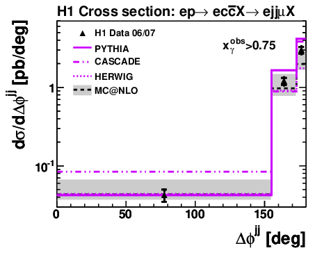
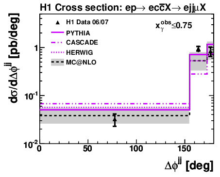

The H1 result is shown in the two rightmost plots. The cross sections are highest for , i.e. for the back-to-back configuration, and drop off towards smaller angles. NLO calculations in the massive scheme [58] and in the massless scheme [48] are compared to the data. Both calculations drop off more steeply than the data towards smaller opening angles. Below the two calculations predict very small contributions, while there are still sizeable ones in the data. A better description is obtained with the LO+PS programs PYTHIA [21] and CASCADE [28]. PYTHIA includes charm excitation processes in resolved-photon events, which give the dominant contribution for and provide a reasonable data description in this region.
The results of the ZEUS analysis [174] are shown in the left and central plots of Fig. 35. Here the azimuthal correlation is measured separately in the 2-parton region and in the 3-or-more-parton region . The data are compared to an NLO calculation [58] in the massive scheme. For the high- region the description is satisfactory. However, in the low- region the NLO calculation is clearly falling below the data for . This is straightforward to understand since a 3-parton final state can not produce an angle between the two leading partons of less than 1919 19 However, in the 3-parton topology one of the leading jets can escape outside of the kinematic region of the measurement. Thus, the softest jet is used instead, which leads to strongly suppressed but non-zero charm contribution for . Correspondingly, at least four partons are needed to populate this region. A massive NLO calculation produces at most three, so an NNLO calculation is needed to fill the gap. Again, a better shape description is obtained by PYTHIA and HERWIG, which can provide several extra partons through parton showering (of which flavour excitation is a part). Thus, the conclusion is again very similar to the above studies with the observable: the NLO calculation is missing a component in the data, which can be effectively described by a LO+PS calculation. As to be expected from this explanation, in the two lower plots the MC@NLO calculation, which complements the 2- and 3-parton NLO matrix elements by parton showering, is able to describe these data well.
6.4.3 Study of hard-scattering angle
In a dedicated analysis [173], using events with a and two jets (entry 8 in Table 3), ZEUS has investigated the scattering angle of the charm quark with respect to the proton direction in the dijet rest frame. The charm quark is identified by the jet to which the reconstructed is associated. The distribution strongly reflects the type of the propagator particle exchanged in the hard interaction:
- •
- •
For a gluon propagator should follow a distribution, i.e. a much steeper rise for . For leading-order processes only the charm-excitation mechanism provides such a contribution (Fig. 6(d)).
The main idea of the analysis is to look for such effects directly in the data. Special cuts are applied in order to ensure a flat acceptance for the distribution over a wide range, extending to as large values of as possible. The invariant mass of the two jets is required to be above 18 GeV. The average pseudorapidity of the two jets, defined as is required to be smaller than 0.7. Note that these cuts yield a much smaller (but still sizeable) contribution at than the one shown in Fig. 33, mainly because they implicitly restrict the two jets to the pseudorapidity region . As intended, this analysis mainly probes 2-parton final states, plus a potential 3rd parton from the photon remnant. In Fig. 36 the differential cross sections are shown as a function of , separately for and .

In the lower half of Fig. 36 the data are compared to massive scheme NLO predictions [58]. For the region the NLO calculation provides a good description of the data over the whole range of , with reasonably small uncertainty. The relatively shallow dependence is consistent with the expectation that this region is dominated by the boson-gluon-fusion graph, where the propagator particle is a charm quark, and for which the prediction is stabilised at NLO by 1-loop virtual corrections. In the region a much stronger rise is visible towards more negative values, and the central region is more strongly depleted. This can be interpreted as a direct proof for sizeable contributions from gluon propagator exchanges such as the charm excitation process (Fig. 6(d)), which at NLO is a tree-level process (Fig. 8(d,e) ). Correspondingly, the NLO uncertainty is much larger. The upper edge of the uncertainty band describes the data reasonably. The strong asymmetry can be attributed to the fact that the charm jet will preferentially be correlated with the incoming photon direction.
The plots in the upper half of Fig. 36 show that the PYTHIA and HERWIG LO+PS MCs with their large excitation contributions are able to describe the data well everywhere. This is particularly true for PYTHIA. For the NLO calculation this means that contributions beyond NLO would probably further improve the description. On the other hand, the CASCADE MC, which attempts to describe hard higher-order topologies by allowing initial state partons to have sizeable transverse momentum, reasonably describes the shapes, but fails to describe the relative normalisation of the low- and high- regions.
6.5 Summary
The charm mass provides a semi-hard QCD scale which already allows the application of perturbative calculations to all of phase space, but which also competes with other, often even harder perturbative scales. Total cross sections for charm photoproduction are reasonably described by such calculations. Single-differential cross sections already provide a good handle to test the applicability of different QCD approximations, although the theoretical uncertainties are mostly much larger than the experimental ones. The theory predictions agree with the data up to the highest accessible transverse momenta, showing no indications that final state resummation corrections are needed for massive calculations.
Double-differential cross sections, in particular those including jets, reveal a partial failure of the massive scheme NLO predictions for the three independent parton-parton kinematic observables , and , which were studied in charm events with a and one or two jets. For certain kinematic regions this can be traced back to the absence of 4-or-more-parton final states in the calculation. The partially large theoretical uncertainties can be explained by the absence of stabilizing virtual corrections for 3-parton final states at this order. The NLO calculations in the massless scheme, where available, do mostly not provide a better description for the observables. The LO+PS MCs PYTHIA and HERWIG, which are often used for acceptance corrections, are able to describe all topologies reasonably, often even very well. The CASCADE MC performs somewhat less well on average.
7 Beauty photoproduction
From the theoretical point of view, the only differences between charm photoproduction as discussed in the previous section and beauty photoproduction are the beauty-quark mass and electric charge. The first suppresses the cross section w.r.t. charm at low values of transverse momentum, while the second suppresses it by about a factor 4 everywhere (Eq. 1). Experimentally, the signal-to-background ratio is thus more challenging, and the available statistics is smaller. Together with the small branching ratio to specific final states, this precludes any attempt to use fully-reconstructed beauty-hadron final states at HERA. On the other hand, the higher mass and longer lifetime compared to charm hadrons increases the tagging efficiency for inclusive tagging methods.
Table 4 summarises all H1 and ZEUS beauty photoproduction measurements. For the reasons explained above, the first such measurements (entries 1 and 2) came several years after the first measurements of charm, focused on beauty jet production, and were severely limited by statistics.
| No. | Analysis | Tag | Ref. | Exp. | Data | Particle | Events |
| |||||||||||
| 1 | + dijets | + | [189] | H1 | 96 |
|
|
||||||||||||
| 2 | + dijets | + | [190] | ZEUS | 96-97 |
|
|
||||||||||||
| 3 | + dijets | + | [191] | ZEUS | 96-00 |
|
|
||||||||||||
| 4 | + dijets | + + | [142] | H1 | 99-00 |
|
|
||||||||||||
| 5 | lifet.+dijets | imp. par. | [141] | H1 | 99-00 |
|
|
||||||||||||
| 6 | + dijets | [176] | ZEUS | 96-00 |
|
|
|||||||||||||
| 7 | +dijets | [192] | ZEUS | 05 |
|
|
|||||||||||||
| 8 | lifet.+dijets | sec. vtx. | [177] | ZEUS | 05 |
|
|
||||||||||||
| 9 | + dijets | +imp.par. | [178] | H1 | 06-07 |
|
|
||||||||||||
| 10 | + | + | [175] | H1 | 98-00 |
|
|
|
|||||||||||
| 11 | + | + | [193] | ZEUS | 96-00 |
|
|
||||||||||||
| 12 | dimuon | + | [194] | ZEUS | 96-00 | all | all | 1(2) | |||||||||||
| 13 | dielectron | + | [195] | H1 | 07 |
7.1 Total cross section for beauty production
Due to their high mass, even beauty quarks at rest in the centre-of-mass system of the partonic interaction still produce reasonably high-momentum muons or electrons, which can be detected, when decaying semileptonically. The forward and backward muon systems allow the detection of such beauty quarks even when they are strongly boosted along the beam direction. Furthermore, the requirement of two such muons, i.e. a double tag, strongly reduces both the light flavour and charm backgrounds.
In a ZEUS analysis [194] these properties were used to measure the total cross section for beauty production in collisions without any cuts, i.e. including both photoproduction and DIS, by pushing the measureable muon phase space to the limit (entry 12 of Table 4). After correcting for muon acceptance and semileptonic branching ratios the resulting total cross section for pair production in collisions at HERA for GeV was determined to be
| (18) |
where the first uncertainty is statistical and the second systematic. The total cross section predicted by next-to-leading-order QCD calculations was obtained in the massive approach by adding the predictions from FMNR [56] and HVQDIS [51] for less than or larger than 1 GeV2, respectively. The resulting cross section for GeV, using the scale choice
| (19) |
is a factor 1.8 lower than the measured value, although compatible within the large uncertainties.
Compareable measurements were obtained in reduced regions of phase space from + muon and dielectron final states (entries 10, 11 and 13 in table 4), and similar results were obtained for the ratio of measured to predicted cross sections (see also corresponding entries in Fig. 37). Since mesons and semi-isolated electrons could only be measured in the more central rapidity range, total cross sections were not extracted.
7.2 Single-differential cross sections
In order to make them compareable with each other, in Fig. 37 almost all available beauty-photoproduction cross sections2020 20 entries 10,5,4,13,2,11,3,6,7,12,8 in table 4, following the order in the figure legend have been translated, using NLO massive QCD calculations, into cross sections for inclusive -quark production as a function of in the kinematic range GeV2, and beauty pseudorapidity . Each data point is displayed at the centroid of the distribution of the quarks entering the measurement bin of the respective analysis, which is mostly a bin in -jet , or, where not available, a bin in muon or electron .

The -quark rather than the -jet has been chosen here because the measurements extend down to very low at which jets can not be usefully defined any more. Two massive NLO [56] theory predictions are given: one with scale choice (dashed), and one with scale choice . The full theory uncertainty band is shown for the latter (for the scale choice see also Section 2.11). It is dominated by the scale variations (independent variation of renormalisation and factorisation scales by factor 2) and by the variation of the pole mass ( GeV). Where not provided directly in the original publications, the data points were obtained using the data/theory ratio of the respective original measurements and rescaling them to the theory prediction in Fig. 37, properly accounting for differences in the respective theory calculation settings.
Within the large uncertainties, reasonable agreement between theory and data is observed over the complete range covering 3 orders of magnitude in the cross section. In particular, as in the charm case, there is no indication for a failure of the predictions at large . There might be a trend that on average, the measurements of the double tagging analyses (, and ), which were already briefly discussed in the total cross-section subscetion, tend to lie a bit above the other measurements which typically require dijet final states. The effect is not very significant, but if taken serious, might indicate that the contribution of quarks not associated to jets might be underestimated by the theory. Unfortunately, currently no measurement is available which directly tests this hypothesis by considering both topologies in a single analysis framework.
All available beauty photoproduction results are represented in this plot, except the results of the very first H1 analysis [189] (entry 1 in Table 4), which has been declared superseded by a more recent analysis [142], and the results of one of the latest H1 analyses [178] (entry 9), for which no comparison to pure NLO predictions was provided.
Double-differential cross sections have not been measured so far. In the future they could best be extracted using the inclusive vertexing approach [177], which offers the best effective statistics (entry 8 in Table 4).


7.3 Measurements of and jet-jet correlations
Several results give insight into correlations between two final state partons in events. The ZEUS analysis of dimuon final states (Fig. 38, entry 11 in Table 4) studies the azimuthal angle difference between muons originating from different quarks, in addition to single-differential distributions. Both the massive NLO predictions and the PYTHIA MC predictions used for acceptance correction show reasonable agreement with the data, in particular in shape.
An H1 analysis of dijet final states in which one of the jets is tagged by a muon from a semileptonic decay (Fig. 39, entry 9 in Table 4) studies the and variables described earlier in the charm section.
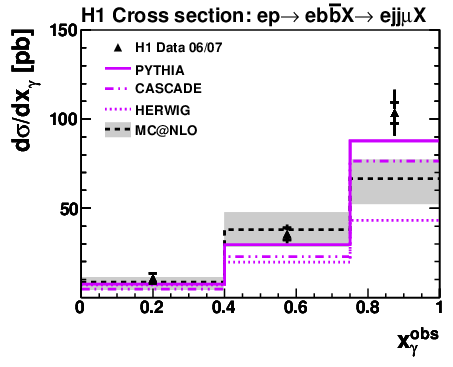
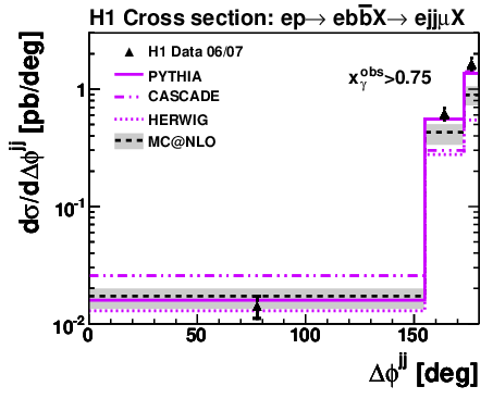
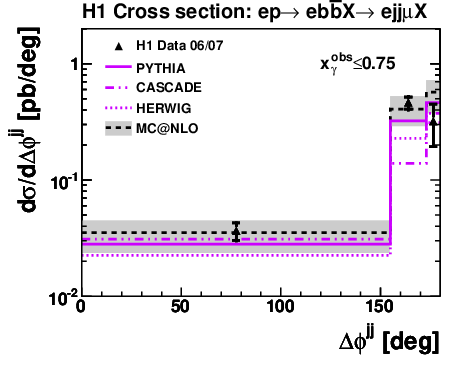
The MC@NLO prediction describes the data, except in the high , high bin. The agreement is thus slightly worse than in the charm case (Fig. 35). PYTHIA agrees everywhere, HERWIG describes the shape but not the normalisation, and CASCADE fails for both. The latter finding is again in qualitative agreement with the charm result. Thus the PYTHIA or HERWIG MCs should preferentially be used for acceptance corrections.
7.4 Summary
Due do the suppression of the cross section by mass and charge, and small branching ratios to exclusive final states, only inclusive or semi-inclusive tagging methods can be used at HERA to measure beauty production. The reasonable acceptance for the detection of hadron decays down to 0 transverse momentum and the coverage of almost the full physically relevant rapidity range allowed the measurement of the total beauty production cross section at HERA. This cross section is higher than, but still compatible with, NLO QCD predictions. Several single differential beauty photoproduction cross sections have also been measured. The measurements from H1 and ZEUS and from different final states agree reasonably well with each other and with QCD predictions from threshold up to the highest accessible transverse momenta. Double differential cross sections have not yet been measured.
8 Charm and beauty production in DIS
In the previous Sections 6 and 7 heavy-flavour production in collisions with the exchange of quasi-real photons was discussed. The production of charm and beauty quarks was also studied in the deeply inelastic scattering regime, which corresponds to photon virtualities . Large photon virtuality provides an additional hard scale in the calculations and allows probing the parton dynamics inside the proton with high resolution. An overview of all measurements is given in Table 5 and Table 6 for charm and beauty production, respectively.
| No. | Analysis | c-Tag | Ref. | Exp. | Data | Particle | Events |
|
| ||||||||||
| 1 | incl. | [196] | H1 | 94 | |||||||||||||||
| incl. | |||||||||||||||||||
| 2 | incl. | [197] | ZEUS | 94 | |||||||||||||||
| 3 | incl. | [169] | H1 | 95-96 | |||||||||||||||
| 4 | incl. | [198] | ZEUS | 96-97 | |||||||||||||||
| 5 | incl. | [199] | H1 | 97 | |||||||||||||||
| 6 | incl. | [200] | ZEUS | 98-00 | |||||||||||||||
| 7 | incl. | mes. + | [147] | H1 | 99-00 | mesons | n.a. | n.a. | |||||||||||
| 8 | incl. | [201] | H1 | 99-00 | |||||||||||||||
| + dijet | Jet1(2) | ||||||||||||||||||
| 9 | incl. | [202] | ZEUS | 98-00 | |||||||||||||||
| 10 | incl. | mes. | [203] | ZEUS | 98-00 | mesons | n.a. | n.a. | |||||||||||
| 11 | incl. | [204] | ZEUS | 96-00 | |||||||||||||||
| incl. | |||||||||||||||||||
| 12 | incl. lifet. | imp. par. | [205] | H1 | 99-00 | Track | |||||||||||||
| 13 | incl. lifet. | imp. par. | [206] | H1 | 99-00 | Track | |||||||||||||
| 14 | incl. | + | [207] | ZEUS | 05 | ||||||||||||||
| 15 | + jet |
|
[208] | ZEUS | 05 |
|
|
|
|||||||||||
| 16 | incl. | [209] | H1 | 04-07 | |||||||||||||||
| 17 | incl. | [144] | H1 | 04-07 | |||||||||||||||
| 18 | incl. | [210] | ZEUS | 04-07 | |||||||||||||||
| 19 | incl. | + | [211] | ZEUS | 04-07 | ||||||||||||||
| 20 | incl. lifet. | + | [149] | H1 | 06-07 | n.a. | Track | n.a. | n.a. | ||||||||||
| 21 | incl. lifet. | jet + + | [212] | H1 | 06-07 | Jet | |||||||||||||
| 22 | incl. lifet. | jet + | [148] | ZEUS | 04-07 | Jet |
| No. | Analysis | c-Tag | Ref. | Exp. | Data | Particle | Events |
|
| |||||||||||
| 1 | + jet | + | [213] | ZEUS | 99-00 |
|
|
|
||||||||||||
| 2 | + jet | + | [142] | H1 | 99-00 |
|
|
|
||||||||||||
| 3 | + jet | + | [214] | ZEUS | 96-00 |
|
|
|
||||||||||||
| 4 | + jet |
|
[208] | ZEUS | 05 |
|
|
|
||||||||||||
| 5 | + jet |
|
[215] | ZEUS | 04-07 | |||||||||||||||
| 6 | + | [193] | ZEUS | 96-00 |
|
|
|
|||||||||||||
| 7 | incl. lifet. | imp. par. | [205] | H1 | 99-00 | Track | ||||||||||||||
| 8 | incl. lifet. | imp. par. | [206] | H1 | 99-00 | Track | ||||||||||||||
| 9 | incl. lifet. | + | [149] | H1 | 06-07 | n.a. | Track | n.a. | n.a. | |||||||||||
| 10 | incl. lifet. | jet + + | [212] | H1 | 06-07 | Jet | ||||||||||||||
| 11 | incl. lifet. | jet + | [148] | ZEUS | 04-07 | Jet |
8.1 Production mechanism
Already in the first H1 [196] and ZEUS [197] measurements in DIS (entries 1 and 2 in Table 5) boson-gluon fusion was clearly identified to be the dominant production mechanism for charm quarks. This was investigated using the distribution of the fractional momentum of mesons in the system, , where denotes the momentum measured in the frame. The data were used to disentangle between BGF and QPM-like models (cf. Fig. 1(a) and Fig. 2). The BGF process produces a pair that recoils against the proton remnant in the frame, while the (massless) QPM produces a single charm quark recoiling against the proton remnant (which contains the other charm quark). Since the meson carries a large fraction of the charm quark momentum, the former model should lead to significantly softer distribution in . Figure 40 shows a comparison of the two models against the ZEUS data.

The observed shape of the cross section in the data proves that BGF is the dominant charm-production process in DIS at HERA. This was quantified in [196] in the leading order QCD picture by setting an upper limit for the fraction of the QPM-like contribution to charm DIS production to be below at C.L.
8.2 Single-differential cross sections
Transition from photoproduction to DIS:
The ZEUS collaboration has studied [202] (entry 9 in Table 5) charm production in the intermediate region between photoproduction and DIS: . The scattered electron was detected with the beampipe calorimeter (BPC) at very small scattering angles. Figure 41(a) shows a comparison of the massive-scheme NLO QCD predictions [51] to these very-low- as well as data [200] (entry 6 in Table 5).


The calculations provide a remarkable description of the drop of the measured cross sections over 5 orders of magnitude from to . The slope of changes with : it is steeper at high , where it is mainly dictated by the photon-propagator dependence , than at low , where an asymptotic dependence is expected. To study this further, the measured electroproduction cross sections were converted into cross sections using the photon flux in the improved Weizsäcker-Williams approximation (see Section 2.9). Figure 41(b) shows the converted DIS as well as the photoproduction cross sections [170] (entry 5 in Table 3). The very-low- measurements are consistent with the photoproduction cross section. The data were fitted with a function . The extracted value was , which is close2121 21 The actual kinematic threshold for a meson pair with only the detected is GeV2. to and is significantly larger than the value obtained from inclusive data, [122].
Performance of the ZMVFNS:
-production single-differential cross sections in DIS have also been used to test available calculations in the massive and massless schemes. Figure 42 shows a comparison of the most precise measurements from H1 [209, 144] (entries 16 and 17 in Table 5) to NLO QCD calculations.


Since the ZMVFNS calculation is only valid in the regime where the charm-quark mass can be neglected, an additional restriction is needed on the transverse momentum in the frame, , on top of the selection outlined in Table 5. This is compareable to the cuts used in the photoproduction analysis, for which the laboratory frame approximately coincides with the system (see Fig. 28). The inelasticity is correlated with the centre-of-mass energy in the frame, (see Eq. (9)), thus the low- region corresponds to the low- region. Therefore, as expected, the ZMVFNS predictions deviate significantly from the massive-scheme calculations at low , where is not , and come close to the FFNS calculations at high . At low the massless-scheme calculations clearly fail to describe the data, while massive predictions are in agreement with the measurement in the whole range. Also for the massive predictions describe the data well within uncertainties, whereas the massless approach significantly overestimates the charm cross section. The data also clearly establish that the ZMVFNS fails to describe heavy-flavour production in DIS at HERA. Similar conclusions were drawn in [201] (entry 8 in Table 5), but with a lower precision of the data.
Event and heavy-flavour kinematics:
Most of the analyses summarised in Tables 5 and 6 studied event, charm and beauty kinematics differentially in the respective fiducial phase spaces. The most precise measurements [209, 144, 210] (entries 16–18 in Table 5) were combined [217] to obtain the most precise charm differential cross sections with essentially no theory uncertainty due to extrapolation to a common phase space. The combination was done with a careful treatment of correlations. As expected, the individual measurements were found to be consistent. The uncorrelated uncertainties were reduced due to effective doubling of statistics, while the correlated systematic uncertainties were reduced through cross-calibration effects between the two experiments. Figure 43(a)–(c) shows a comparison of massive-scheme NLO QCD predictions [51] to the combined single-differential cross sections.


The predictions describe the data very well within uncertainties. However, the data reach precision over a large fraction of the measured phase-space, whereas the typical theory uncertainty ranges from at low to at high . The theory uncertainty is dominated by the independent variation of the and scales, the uncertainty on the charm-quark pole mass and variations of the fragmentation model. Therefore, higher-order massive-scheme NNLO calculations and an improved fragmentation model for these predictions are needed to fully exploit the potential of these data. In addition, theory uncertainties were studied in detail and a “customised” prediction was obtained by a variation of the theory parameters within their uncertainties, to show that the calculations can simultanously provide a good description of the shape and normalisation of all measured distributions with a single set of parameters. This led to a renormalisation scale reduced by a factor 2 (see also Section 2.11), the charm-quark pole mass reduced to and to a change of fragmentation parameters, all within the nominal uncertainties.
Moreover, differential cross sections of other mesons as well as of leptons from heavy-flavour decays and of heavy flavour jets were measured. In particular, Fig. 43(d) shows the differential cross section [204] (entry 11 in Table 5) measured down to . The measurement was done in the decay channel. The presence of a neutral strange hadron in the decay resulted in a reasonable signal-to-background ratio even at very low transverse momentum of the . The data were found to be described by the massive NLO QCD calculations within about two standard deviations.
Furthermore, parton-parton correlations have been studied in -tagged events [201] (entry 8 in Table 5). The conclusions are similar to those obtained from the respective photoproduction measurements. In general the massive QCD calculations provide a good description apart from the region of small and very large between the two leading jets in the event (not shown).
Inclusive lifetime tagging (entries 21, 22 in Table 5) allowed the extension of the kinematic range of charm measurements up to (not shown), which roughly corresponds to , where the statistics of fully reconstructed charm mesons becomes poor. Good agreement is again observed.
Figure 44 shows the corresponding single-differential jet cross sections for beauty production in DIS [148] (entries 11 and 22 in Tables 6 and 5, respectively).


The lifetime-tagging technique together with the reconstruction of the vertex mass were used to extract charm- and beauty-jet cross sections simultaneously. This measurement was selected since it has the highest statistical significance for beauty-quark production, as can be seen from the last column of Table 6. The typical precision reached in the data is and is comparable to the theory uncertainties. The massive-scheme NLO QCD calculations provide a good description of the shape and normalisation of the measured cross sections.
8.3 Double-differential cross sections
The large collected data samples allowed measurements of double-differential heavy-flavour cross sections, to study the correlations between various kinematic variables.
The H1 collaboration has studied [201] (entry 8 in Table 5) the cross section as a function of in different ranges, complementing the measurements in the photoproduction regime discussed in Section 6.4.1. It was shown that the amount of higher order contributions included in the massive NLO calculations, including topologies which would be called “flavour excitation” in the leading order picture, is enough to describe the data for different , while the BGF-only component of the RAPGAP Monte Carlo can describe the measurement for after rescaling, but fails to describe the shape observed in the data at lower (not shown here). This is to be expected, since in this “photoproduction-like” region (see Fig. 41) the “flavour excitation” component will then be missing.
Using the full HERA II data sample, cross sections have been measured by H1 [144] (entry 17 in Table 5) as a function of the pseudorapidity in the laboratory frame, , in bins of the transverse momentum in the centre-of-mass frame, . Figure 45 shows a comparison of the massive NLO QCD predictions to the data.

At large , production in the backward region is very suppressed, while at low the distribution is rather flat in the phase space of the measurement. The massive-scheme NLO predictions provide a good description of the data. The predictions depend only very little on the proton PDFs used for the calculation.
In most of the analyses summarised in Tables 5 and 6 the double-differential cross sections in and or and were also measured. These measurements allowed dedicated studies of the inclusive heavy-flavour event kinematics which can be expressed in terms of the charm reduced cross sections, or of the charm contribution to the structure function (see Section 8.4). Figure 46 shows the combined double-differential cross sections as a function of and [217].

Massive-scheme NLO QCD predictions provide a good description of these cross sections in the full range in between and . The theoretical uncertainties decrease with increasing . For the theoretical uncertainties are larger than those of the measured cross sections. Similar to the single-differential distributions shown in Fig. 43, the theoretical uncertainties are dominated by the scale variations, the uncertainty on the charm-quark pole mass and the variation of the fragmentation model. A higher-order calculation with improved fragmentation model is needed to achieve a theoretical precision similar to the data.
8.4 Proton structure functions and reduced cross sections
The measured double-differential DIS cross sections of heavy-flavour production as a function of and or and were used to extract the heavy-flavour reduced cross sections, , or the heavy-flavour contribution to the proton structure function , , where is either or . As discussed in Section 2.8, the inclusive double-differential cross sections of heavy-flavour production can be expressed in terms of or and . In measurements of the small contribution arising from was subtracted relying on theory, corresponding to a correction of up to . The extraction from the measured cross sections requires an extrapolation from the experimentally accessible kinematic region in and and a particular final state to the full phase space of heavy quarks. The extrapolation was done either using the massive-scheme NLO QCD calculations or LO+PS Monte Carlo simulations. Since this procedure relies on the description of kinematic distributions by predictions, a non-negligible theoretical uncertainty was introduced. This additional uncertainty was estimated by varying the parameters in the calculations which affect the shapes of the kinematic distributions.
The and values extracted from measurements performed with different experimental techniques and different detectors can be directly compared. Such measurements are complementary to each other due to different dominant sources of systematics, mostly independent statistics and different kinematic coverage, resulting in somewhat different theoretical uncertainties due to extrapolation. For instance, for the measurements the dominant systematics in the H1 inclusive vertexing analysis (entry 20 in Table 5) is due to the treatment of the light-flavour component, while in the H1 HERA II measurement (entry 17 in Table 5) the dominant systematics is due to the modelling of the tracking efficiency. The ZEUS analysis of charm semileptonic decays (entry 15 in Table 5) has yet completely different systematics. Therefore, a combination of measurements with such different techniques allows a significant reduction not only of statistical and uncorrelated but also of correlated systematic and extrapolation uncertainties.

Figure 47 shows a comparison of H1 and ZEUS measurements of the charm reduced cross sections2222 22 entries 4,6,8,12,13,14,15,16,17,20 in Table 5 as well as the milestone result of their combination [84]. The combination accounts for correlations of the systematic uncertainties among the different input data sets. The individual measurements show good consistency, with a value of for degrees of freedom. The combined data are significantly more precise than any of the input data sets. Figure 47 also highlights the advantages of different tagging techniques: while has superior precision at low due to better signal-to-background ratio, the inclusive vertexing analysis with lifetime tagging dominates at high due to the larger accessible statistics. The final total precision of the combined charm reduced cross sections is on average and reaches at low and medium . This corresponds to a factor 2 improvement over the most precise data set in the combination.


Additionally, new statistically independent measurements of charm production have been published (entries 18,19 and 22 in Table 5), in particular the ZEUS measurement with HERA II data. In Fig. 48 the combined [84] and individual measurements of (entries 3–5, 7–9, 11 in Table 6) are compared to NLO and NNLO QCD predictions.
The beauty measurements are all in good agreement with each other and the most precise data were obtained with inclusive lifetime tagging. The NLO QCD prediction in the GMVFNS approach based on HERAPDF1.5 [42] is common for the two comparisons. The good agreement between these predictions and the heavy-flavour data shows that the gluon density, which in HERAPDF1.5 is extracted from the scaling violations of , is adequate for the description of these gluon-induced production processes. Other GMVFNS predictions were also compared to the combined charm reduced cross sections (not shown). The best description of the data was provided by predictions including partial corrections, while predictions including terms agreed well with the data and predictions including have shown the largest deviations [84]. The theoretical uncertainty for and increases at low and is dominated by the variation. This indicates that the low- data are sensitive to the value of the heavy-quark mass used in the calculation, which was exploited to extract the optimal values for different GMVFNS schemes as well as to measure the running heavy-quark masses (see Section 9.2).
Fig. 49 shows the fraction of the heavy-flavour component in the total inclusive DIS cross section: and /.


As expected, the heavy-flavour fractions increase with increasing . For , the asymptotic limit is approached towards for charm and for beauty. The charm and beauty fractions in the high- data come close to and , respectively, stressing the importance of the heavy-flavour component for the description of inclusive DIS. The observed suppression of the heavy-flavour fractions for originates from the rising importance of the valence-quark contribution to the inclusive DIS cross section in this kinematic domain.
8.5 Summary
Large photon virtuality provides an additional hard scale in the QCD calculations of heavy flavour production and allows probing the parton dynamics inside the proton more directly than photoproduction. The dominant contribution to the charm and beauty cross sections arises from photon-gluon fusion. For , where the photon virtuality is the dominant hard scale, the cross-section behaviour is similar to the one of the inclusive cross section for deeply inelastic scattering. At high and low , the naively expected charm and beauty contributions of and are asymptotically approached. For , where the quark mass is the dominant hard scale, the cross section behaves essentially like photoproduction, i.e. the photon can be approximated to be quasi-real. NLO QCD predictions using zero-mass schemes (ZMVFNS) fail to describe the data in the vicinity of or below the so-called “flavour threshold” at . NLO QCD predictions in the massive scheme (FFNS) give a good description of heavy flavour production at HERA over the complete accessible kinematic range. NLO predictions in variable flavour number schemes (GMVFNS) are only available for inclusive quantitities, and perform about equally well. There is no indication for the need of resummation of terms at HERA energies. In particular for charm, the uncertainties from QCD corrections beyond NLO and from the modelling of fragmentation are considerably larger than the experimental uncertainties of the measured cross sections. Improved QCD calculations would therefore be highly welcome.
9 Measurement of QCD parameters, proton structure, and impact on LHC and other experiments
So far the emphasis was on direct cross-section measurements from the HERA data and on the comparison to and performance of different theoretical approximations for the perturbative QCD expansion. In this section the extraction of more fundamental QCD parameters and parametrisations will be discussed, which are of direct relevance to all high energy physics processes and to the Standard Model of particle physics in general.
9.1 Measurement of charm fragmentation functions and fragmentation fractions
As outlined in Section 2.10, fragmentation fractions, i.e. the probability of a quark of a given flavour to form a specific final state hadron, and fragmentation functions, parametrising the fraction of the energy or momentum of the final state quark which will be taken by the final state hadron, are essential to relate theoretical QCD calculations at parton level to measurable hadronic final states.
Studies of the fragmentation process are based on a complete reconstruction of the final-state hadron. The statistics accessible at HERA for fully-reconstructed beauty hadrons is extremely low due to the moderate beauty-production cross section and small branching ratios. On the other hand, HERA is effectively a charm factory, with about charm events recorded to tape. Therefore, only the fragmentation of charm quarks has been studied by H1 and ZEUS. Charm fragmentation has been studied in both the DIS and photoproduction regimes. A comparison between these results and measurements provides a so far unique test of the fragmentation universality in the heavy-flavour sector for colour-neutral (electromagnetic) vs. coloured (strongly interacting) initial states.
9.1.1 Charm fragmentation function
The explicit reconstruction of a meson in the final state has the optimal signal sensitivity of all fully reconstructed charm final states (cf. Table 3 and Table 5). Thus, it has been used for studies of the non-perturbative charm fragmentation function (Section 2.10). Since the momentum of the charm quark is not measured in the detector, the fragmentation function is not a directly accessible quantity. It can be approximated either by jets to which a reconstructed meson is associated (for high- events) or by the overall energy flow in the event hemisphere around the (for production close to the kinematic threshold). Parameters of the fragmentation function were extracted from the data by fitting corresponding predictions to the measured normalised differential cross sections as a function of
and
for the jet and hemisphere methods, respectively. The tuning of the fragmentation parameters was done based on Monte Carlo simulations [21, 23] with similar JETSET [24] settings or on NLO QCD calculations using the same ‘‘heavy quark’’ definition and similar schemes for the cancellation of collinear and infrared divergences2323 23 Due to the heavy quark masses most of these terms are not really divergent. Nevertheless, events with “similar” topologies and large but almost cancelling weights are produced in correlated groups. in photoproduction and DIS [56, 51].
The H1 [220] and ZEUS [221] measurements were done in the DIS and photoproduction regimes, respectively, utilising HERA I data sets. The H1 experiment investigated both the high and the threshold regions, in order to cover the largest possible phase space, while ZEUS restricted the measurement to the high- regime, in order to reach small values without strongly biasing the distributions, and in order to minimise perturbative fragmentation factorisation effects within the data set. This led to H1 selecting jets with in the rest-frame and ZEUS cutting on for jets in the laboratory frame. Figure 50 shows the measured normalised differential cross sections as well as predictions after tuning of the fragmentation model.


The extracted parameters of the fragmentation functions for the HVQDIS and FMNR NLO calculations, which should also be applicable to the conceptually similar MNR [60] calculations in hadroproduction, are presented in Table 7.
| H1 [220] | ZEUS [221] | |||
| kinematics | threshold | high | high | |
| method | hem | hem | jet | jet |
| Kartvelishvili [95] | ||||
| n.a. | ||||
| Peterson [94] | ||||
| n.a. | ||||
A few observations can be made from the distributions:
- •
As expected, due to the high quark mass, a charm meson retains a large fraction of the momentum of a charm quark. Therefore, the charm fragmentation is much harder than that of light hadrons.
- •
The fragmentation of charm quarks to mesons near to the kinematic threshold is harder than in the region away from the threshold (cf. Fig. 50 (b) and (c)). This can be qualitatively understood as a consequence of the fact that the phase space available for the production of additional particles is smaller near threshold. As a result, the fragmentation parameters extracted in the two kinematic regions are significantly different. This leads to the conclusion that the different kinematic regimes can not be described simultaneously within the framework of the independent fragmentation function. This is to be expected, since the nonperturbative phase space suppression is incompletely modeled in this approach.
- •
NLO QCD calculations in conjunction with an independent fragmentation fail to describe the data close to the kinematic threshold: (see Fig. 50 (c) and Table 7). However, in the same phase space MC simulations can be tuned to provide a reasonable description of the distribution in the data: (see Fig. 50 (d)). This might be due to the proper treatment of phase space effects in the MC, which are missing in the independent fragmentation approach used for the NLO predictions.
- •
The Peterson fragmentation provides a much worse description of the data than the Kartvelishvili function. This has also been observed elsewhere [222].
- •
The jet and hemisphere methods in the region where both are applicable, i.e. away from the threshold, yield similar results for the Kartvelishvili parametrisation, while they remain somewhat different in the Peterson case. Thus again, the Kartvelishvili parameterisation seems to be preferred.
For some recent measurements [84, 144, 204, 209, 210, 211, 217], these results have been used explicitly to model the fragmentation for the comparison of theoretical predictions to the charm HERA data (see Section 8) and for the extrapolation to the full phase space in the context of the extraction of the charm reduced cross sections (see Section 8 and Section 9.2). This has shown that there are significant theory uncertainties due to fragmentation. A consistent phenomenological reanalysis of the H1 and ZEUS data is needed in order to resolve the differences observed in different kinematic domains, which originate from neglecting perturbative evolution and phase space effects, hopefully resulting in an important reduction of the related theory uncertainties. It is worth mentioning that the complete HERA II dataset, which has not yet been analysed in this context, is available in principle for this purpose.
| H1 [220] | ZEUS [221] | |||
| kinematics | threshold | high | high | |
| method | hem | hem | jet | jet |
| Kartvelishvili | ||||
| n.a. | ||||
| n.a. | ||||
| Peterson | ||||
| n.a. | ||||
Table 8 shows the equivalent results extracted from LO+PS MCs using the “default” JETSET settings as used e.g. by the PYTHIA and RAPGAP MCs. In this case a perturbative evolution of the fragmentation function is partially included through the parton showering, and phase space corrections are applied. Despite the poor , the Peterson parameters extracted from the intermediate and high jet samples now agree with each other, as well as with the corresponding default parameter 0.05 extracted from collisions [221]. This confirms the universality of the nonperturbative part of fragmentation. Kartvelishvili parameters are unfortunately not available for all data sets and can hence not be compared. Near threshold, even the MC model does not yield the same fragmentation parameters, and the is generally bad. This indicates that still not all threshold effects might have been fully accounted for.
9.1.2 Charm fragmentation fractions and ratios
The fractions of quarks hadronising into a particular charm hadron, , have been measured by H1 and ZEUS in the DIS [147, 203, 204] and photoproduction [145, 143] regimes. The measurements were done for , , , and based on full reconstruction of the charm-hadron decays. The fragmentation fractions were extracted from integrated visible cross sections. The typical fiducial phase space of the charm hadrons was defined by and . The fragmentation fractions were extracted with the additional constraint that the sum of the fractions for all weakly-decaying open-charm hadrons (i.e. the ground states from the point of view of strong and electromagentic interactions) has to be equal to unity. This was done by a constrained fit in H1 [147] and by an advanced procedure called equivalent phase space treatment in ZEUS [203]. In addition to direct production, such experimentally measured fragmentation fractions include also all possible decay chains of excited charm hadrons.
Figure 51 shows a compilation of all available charm fragmentation fraction measurements. The HERA data are compared to an average of measurements [224, 225]. To allow a direct comparison, all measurements have been corrected [226] to the decay branching fractions from PDG 2010 [227].

The HERA data reach very high precision, benefiting from a partial cancellation of some systematic uncertainties in the ratio. In particular, the recent ZEUS measurement [143] is based on the full HERA II data sample and made use of the finalised tracking with lifetime tagging for , and . This allowed to reduce both statistical and systematic uncertainties. The ultimate precision achieved with ZEUS HERA II data alone is fully competitive with the precision of the average from several experiments. All data from DIS, photoproduction and collisions are in agreement within the high accuracy of the data. This demonstrates that the charm fragmentation fractions are independent of the production mechanism, and therefore supports the hypothesis of universality of heavy-quark fragmentation. The agreement between the fragmentation fractions has been checked quantitatively in the context of a combination [226].
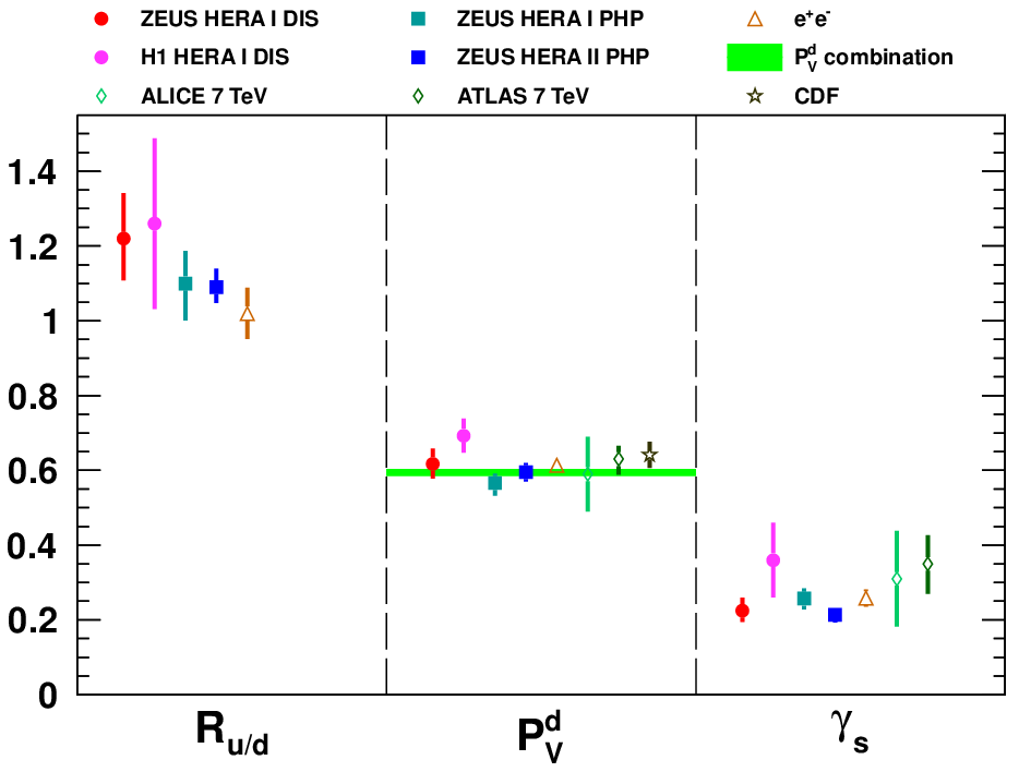
In addition to the fragmentation fractions, various charm fragmentation ratios were extracted: the ratio of the neutral to charged -meson production rates, , the fraction of the charged D mesons produced in a vector state, , and the strangeness-suppression factor, . Figure 52 shows a comparison of HERA measurements [143, 145, 147, 203, 204] with results obtained in collisions (numbers quoted in [203] using average from [224]) and hadroproduction by CDF [228], ALICE [229, 230] and ATLAS [225]. Also shown is a global average of results from , photo- and hadroproduction [231]2424 24 The paper as well as other recent measurements [228, 229, 225] report values, which correspond to the fraction of charged and neutral D mesons produced in the vector state. However the measurements rely on isospin symmetry assumption, which makes identical to ., which also includes some , and CDF data shown separately. Note, that the uncertainty of the average is driven by the result from the WA92 experiment [232], which is quoted with statistical uncertainty only, i.e. treating all systematic uncertainties, including the branching-ratio uncertainty, as correlated between and . The fragmentation ratios extracted from HERA, and hadroproduction data agree within experimental uncertainties. The ultimate precision achieved with the full HERA II data set is competitive with the most precise measurements in other experiments. Various simple theory expectations can be tested against the data. The measurements are slightly above, but still in agreement within uncertainties, with the isospin invariance expectation of unity. The measurements are smaller than the naive spin-counting expectation and the string fragmentation prediction [233, 234].
Excited charm mesons have also been studied with the ZEUS detector using the HERA I [235] and HERA II [236] datasets. Some parameters of the orbitally-excited charm states with and with as well as charm-strange state were measured. The masses and widths were found to be in good agreement between the two measurements and with the PDG average. The helicity parameters for and were found to be in agreement with measurements. The measured parameter was found to prefer a mixture of and waves in the decay to , although it is also consistent with a pure wave. In addition, fragmentation fractions and ratios of branching ratios were extracted. For some parameters HERA can provide important or even so far unique information. For example, the fragmentation fractions for the studied excited mesons are so far very poorly experimentally determined. The and fragmentation fractions were measured for the first time [236]:
9.2 Measurement of parton density functions
The gluon PDF at low- and medium- values is mostly constrained by the scaling violations of the inclusive structure function . In contrast, heavy-quark production at HERA provides a direct probe of the gluon momentum distribution in the proton through the process. Such direct measurements are complementary to the indirect approach.
Already the very early charm measurements were used to directly extract the gluon PDF, as was done by the H1 collaboration in [169]. The gluon densities extracted from the charm data were found to be in agreement with the result of a QCD analysis of inclusive measurements, although the charm measurement was limited by statistics.
The recent combined charm DIS data [84] were also used in a QCD analysis [84] together with the combined inclusive HERA I DIS cross sections [218]. Only the data with were used in the analysis to assure applicability of pQCD calculations. The analysis was performed at NLO using the HERAFitter package [237, 218, 238] and closely followed the HERAPDF1.0 prescription [218]. Various implementations of the NLO GMVFNS approach were used and the role of the value of the charm quark mass parameter (see Section 2.7), , was studied. For each heavy-flavour scheme a number of PDF fits was performed to scan of the PDF fit as a function of . From the scan the optimal value, , of the charm-quark mass parameter in a given scheme was determined by the minimum of the and the corresponding fit uncertainty2525 25 This minimisation uncertainty is usually referred to as the “experimental” uncertainty in the HERAPDF context [218, 84]. However, it can absorb some other sources of uncertainties, e.g. variations of PDF parametrisation. Therefore, the more general term “fit uncertainty” is used here. was evaluated from the variation. The procedure is illustrated in Fig. 54(a) which shows the fit to the inclusive DIS data alone and together with . The inclusive DIS cross sections alone only weakly constrain , indicated by the shallowness of the distribution. The charm DIS cross sections provide the required constraint to extract . Additionally, for each GMVFNS approach the model and parametrisation assumptions in the fits were varied one-by-one and the corresponding scan as a function of was repeated. The difference between obtained with the default assumptions and the result of each variation was taken as the corresponding source of uncertainty. The dominant contribution to the uncertainty was found to come from the variation of the minimum value for inclusive DIS data used in the fit.
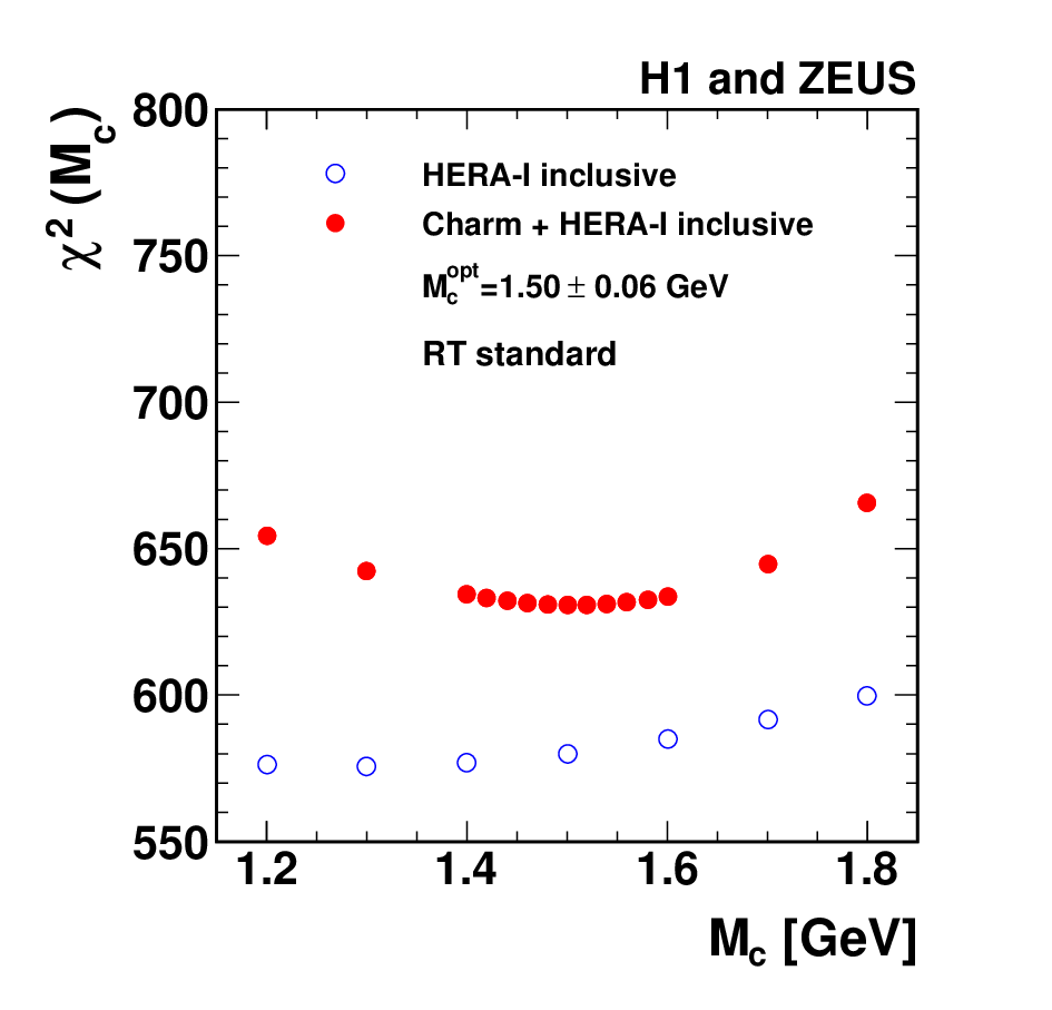

Figure 54(b) shows the distributions as a function of obtained from fits to the inclusive HERA I data and the combined for all variable-flavour-number schemes considered. All schemes yield similar minimal values, however at quite different values of . The resulting values of are given in Table 9 together with the evaluated uncertainties, the minimal total values and the contribution from the charm data. The ACOT-full scheme provides the best global description of the inclusive and charm data together, while the RT optimised scheme yields the best description of the charm data alone. The fits in the S-ACOT- scheme result in a very low value of compared to other approaches. Since this scheme only includes a leading-order approximation of heavy-flavour production at the order considered here (see Table 1), effectively no distinction is made between pole or running mass.
| Scheme | |||
|---|---|---|---|
| [GeV] | + | ||
| RT standard | |||
| RT optimised | |||
| ACOT-full | |||
| S-ACOT- | |||
| ZMVFNS |
All NLO VFNS predictions using corresponding values for each scheme provide a similarly good description of the data [84].
Figure 54 shows the PDFs extracted from the fit to the inclusive DIS data alone and together with the data in the RT optimised VFNS2626 26 Similar observations were made with other schemes.. A comparison of the extracted PDF uncertainties yields the following conclusions about the impact of the data [84]:
- •
the uncertainty on the gluon PDF was reduced, mostly due to a reduction of the parametrisation uncertainty due to the additional constraints that the charm data introduce due to the BGF process;
- •
the uncertainty on the charm-quark PDF is considerably reduced due to the constrained range of . The variation was set to for the fit to the inclusive data only and was defined by the evaluated total uncertainties as given in Table 9 for the fit including the charm data;
- •
the uncertainty on the up-quark sea PDF was correspondingly reduced, because the inclusive data constrain the sum of up- and charm-quark sea;
- •
the uncertainty on the down-quark sea was also reduced because it was constrained to be equal to the up-quark sea at low ;
- •
the uncertainties on the valence-quark and strange-quark sea PDFs were almost unaffected;
- •
the central PDFs were not altered significantly and were found to be within the uncertainties of the PDFs based on inclusive data only. This reflects the good description of the charm data by the default PDFs (section 8.4).
By now, the combined charm reduced cross sections [84] have been used in QCD analyses by various PDF-fitting groups [239, 240, 33, 241, 242, 243, 244]. They are an important ingredient to constrain the proton flavour composition (see also next section) and to stabilise its gluon content. The latter is especially important for Higgs production at the LHC, for which the dominant process is gluon-gluon fusion via an intermediate top-quark loop. Measuring this process precisely, in combination with a precise knowledge of the gluon content of the proton, allows the extraction of a precise measurement of the Higgs-top Yukawa coupling.
Instead focusing on the low- range, the HERA charm and beauty data have recently been used in conjunction with charm and beauty data from LHCb to constrain the gluon distribution down to [245]. This region is particularly relevant for the prediction of cross sections for processes occurring in cosmic ray interactions.
9.3 Proton flavour composition and W/Z/H production at LHC
In the previous section it was outlined how the inclusion of charm data into GMVNFS PDF fits, and in particular the constraint on the charm quark mass parameter derived from these data, imposes constraints on the gluon content (relevant e.g. for Higgs production) and on the flavour composition of the quarks in the proton. This, in turn, affects theoretical predictions for processes which are sensitive to this flavour composition, such as the production for W and Z bosons at LHC.
Figure 55 shows NLO predictions for and production at LHC for PDFs extracted in different heavy flavour schemes as discussed in Section 9.2, as a function of the charm quark mass parameter used in the PDF fit. For fixed , these predictions differ by about . The dependence on is opposite to what one would naively expect (see also Fig. 54). A higher charm mass leads to less charm in the proton (fewer gluons split) but to a higher gluon density. This in turn increases the amount of and sea quarks in the proton, even more so since the total sea is constrained by the inclusive proton structure functions. The larger number of and quarks overcompensates the smaller number of quarks and leads to an increase of the and cross sections as shown in Fig. 55. The fit in Fig. 54 actually led to a smaller charm mass than the default, therefore the effect on the PDF was opposite.


The stars in Fig. 55 indicate the cross section predictions for the optimal mass for each heavy flavour scheme, as extracted from the charm data in Fig. 54(b). All predictions then coincide to within , independent of the heavy flavour scheme used. This demonstrates that using the optimal mass for each scheme which best fits the HERA charm data stabilises the flavour composition in the proton, and leads to a reduction of this contribution to the cross section uncertainty by about a factor 3. To minimise the uncertaities arising from the charm and beauty masses, for GMVFNS schemes it is thus strongly recommended to use the optimal mass parameters as derived from the heavy-flavour structure-function data rather than a mass obtained from external considerations.
A similar analysis for beauty, which remains to be done, will in addition yield experimental constraints on the PDF in the framework of 5-flavour PDFs for LHC, which are so far constrained by theory only. This in turn will be relevant e.g. for a future measurement of the Higgs- Yukawa coupling from associated Higgs- production.
9.4 Measurements of the charm-quark mass and its running
The sensitivity of the HERA reduced charm cross sections to the charm-quark mass, already partially studied in Section 9.2, can be used to measure the charm quark mass appearing in perturbative QCD, whose value depends on the renormalisation scheme within which it is being evaluated. The two mass definitions which are most commonly used are the pole mass and the running mass (Section 2.4). Since the mass is perturbatively better defined, recent charm mass measurements concentrate on this renormalization scheme. The FFNS scheme (Section 2.6) is most suited for this evaluation, since it fully accounts for mass effects without any additional free parameters. FFNS calculations of the reduced cross section in this scheme exist at NLO and partial NNLO [62, 32]. All results quoted in the following are obtained from these calculations unless otherwise quoted.
The first determination of the charm-quark mass [246], from a subset of charm data from the H1 collaboration, in which also the details of the theoretical framework are given, obtained
| (20) |
at NLO, and
| (21) |
at partial NNLO, where the last term reflects a very conservative estimate of the evaluation of the uncertainties of the NNLO approximation.

Figure 56 shows the comparison of predictions of the ABKM group [46], using the above mass values as central values, to the combined HERA charm data [84] discussed in Section 8.4, which have smaller uncertainties than the data used for the initial measurement. Very good agreement is observed for both NLO and partial NNLO.


The H1 and ZEUS collaborations have used a fit to these data (Fig. 57(left)), using the kinematic region , to obtain the NLO measurement [84]
| (22) |
This result has a slightly more elaborate evaluation of the uncertainties related to the data extrapolation as well as other model and parametrisation uncertainties, while it does not include uncertainties on the normalisation of the cross section predictions due to QCD scale variations.
The same data where then used by the ABM group and collaborators [239] to reobtain similar evaluations,
| (23) |
at NLO, and
| (24) |
at partial NNLO. The smaller central NLO value and the smaller uncertainty are mainly due to the fact that the charm data from the lowest bin were included. A correlated measurement of and the strong coupling constant [247] was also obtained (Fig. 57(right)). In particular for the NLO case, the correlation between and is non-negligible.
They were also used by the CTEQ group [33] to derive the mass in the context of the S-ACOT- VFNS, using charm matrix elements to one-loop order in the massive part of the calculation. The result
| (25) |
exhibits a larger uncertainty than the previous extractions due to the additional uncertainty from the variation of the (single) free parameter of this VFNS scheme, and due to conversions between the pole and running masses in the extraction process.
All these results from a predominantly space-like perturbative process are consistent with each other and with the world average [146]
| (26) |
obtained from lattice QCD and time-like processes. This is a highly nontrivial triumph of QCD. Some of the above measurements are now included in the latest world average [30], and further improvements on both the experimental and theoretical sides have the potential to further improve the corresponding precision.
In a recent preliminary result [248] the same data have again been used to determine the actual scale dependence (‘running’) of the charm-quark mass in the scheme, according to Eq. (13). For this purpose, the charm data were subdivided into 6 different ranges, for which the charm mass was extracted separately at the scale , where is the average of each range. The result is shown in Fig. 58. This is the first explicit measurement of the scale dependence of the charm quark mass.

9.5 Measurement of the beauty-quark mass and its running
Using the same approach as outlined above for charm, the ZEUS collaboration has used a fit (Fig. 59) to the beauty reduced-cross-section data [148]

to extract the value of the beauty-quark running mass at NLO,
| (27) |
where the theoretical uncertainty is dominated by the scale variation uncertainty. This is the first such extraction from HERA data, and agrees well with the world average [146]
| (28) |
Figure 60 shows this result, translated to the scale , compared to the PDG value and its expected running and to values extracted from LEP data at the scale . The expected running of the beauty-quark mass is confirmed. This is a nontrivial test of the basics of QCD.

9.6 Summary
Heavy flavour physics at HERA yields many results which are of interest for particle physics in general. The usage of HERA as a “charm factory” generates world-class information on charm fragmentation functions and fragmentation fractions and allows tests of the fragmentation universality. The constraints on PDFs from charm data, and to a lesser extent also from beauty data, help to reduce uncertainties for important cross sections at LHC, such as heavy flavour, W/Z and Higgs production. Constraints on the latter are important for the measurement of the Higgs Yukawa couplings. More directly, the charm and beauty DIS data have been used to extract well defined measurements of the charm- and beauty-quark masses, which enter the world average. The running of the charm-quark mass has been measured for the first time ever. By comparing with LEP data, the running of the beauty quark mass has also been confirmed. In general, the good agreement of QCD predictions with the data support the applicability of the HERA results to all particle physics applications for which they might be directly or indirectly relevant.
10 Summary and outlook
Charm and beauty production at HERA are a great laboratory to test the theory of heavy flavour production in the framework of perturbative QCD and to measure some of its parameters. The occurrence of different possibilities to treat the heavy quark masses in the PDF, matrix element and fragmentation parts of the calculation introduces a significant level of complexity into the corresponding QCD calculations, in addition to the usual scheme and scale choices. Confronting such different choices with data can be helpful to understand the effects of different ways to truncate the perturbative series and to evaluate their impact on the measurement of fundamental parameters, both at HERA and at other colliders.
HERA was the first and so far only high energy collider. The heavy flavour results discussed in this review were obtained with the H1 and ZEUS detectors which were well suited for the detection of heavy flavoured particles. Adding the luminosities from the two collider experiments, a total luminosity of about was collected.
The availability of many different charm and beauty tagging methods allows results to be obtained through several different final states with different systematics. In addition to the statistical benefit from combining different samples, such combinations also profit from cross calibrations of the systematics from different methods and experiments.
Due to the high top mass, the only top final state which might have been detectable at HERA is single top production with non-Standard-Model couplings. No signal is seen, and the coupling limits derived are competitive.
The charm (beauty) quark masses provide semi-hard (hard) QCD scales which allow the succesful application of perturbative calculations over the complete phase space. However, these masses also compete with other, often even harder perturbative scales. Total cross sections for charm photoproduction and the total cross section for beauty production (including photoproduction and deeply inelastic scattering) are reasonably described by perturbative calculations at next-to-leading order (NLO). Single-differential cross sections already provide a good handle to test the applicability of different QCD approximations, although the theoretical uncertainties are mostly much larger than the experimental ones. The theory predictions agree with the data up to the highest accessible transverse momenta or photon vitualities, showing no indications that final state resummation corrections are needed for massive calculations in the HERA kinematical domain. Double-differential cross sections, in particular those including jets, reveal a partial failure of the massive scheme NLO predictions for kinematic observables which would need final states with four or more partons in the calculation. Although statistics and therefore precision is higher for photoproduction, qualitatively very similar conclusions are obtained for photoproduction and deeply inelastic scattering (DIS). The NLO calculations in the massless scheme, where available, do mostly not provide a better description for the observables, and clearly fail for some DIS observables. The LO+PS MCs PYTHIA and HERWIG, which are often used for acceptance corrections, are able to describe all topologies reasonably, often even very well. The CASCADE -factorisation MC performs somewhat less well on average.
In DIS, the large photon virtuality provides an additional hard scale in the QCD calculations of heavy flavour production and allows probing the parton dynamics inside the proton more directly than in photoproduction. The dominant contribution to the charm and beauty cross sections arises from photon-gluon fusion. For , where the photon virtuality is the dominant hard scale, the cross-section behaviour is similar to the one of the inclusive cross section for deeply inelastic scattering. At high and low , the naively expected charm and beauty contributions of and are asymptotically approached. NLO QCD predictions in the massive scheme (FFNS) give a good description of heavy flavour production at HERA in DIS over the complete accessible kinematic range. NLO predictions in variable-flavour-number schemes (GMVFNS) are only available for inclusive quantities, and perform about equally well.
In particular for charm, the uncertainties from QCD corrections beyond NLO and from the modelling of fragmentation are considerably larger than the experimental uncertainties of the measured cross sections. Improved QCD calculations would therefore be highly welcome.
Heavy flavour physics at HERA yields many results which are of interest for particle physics in general. The usage of HERA as a “charm factory” generates world-class information on charm fragmentation functions and fragmentation fractions and allows tests of the fragmentation universality. The constraints on proton parton distribution functions (PDFs) from charm and beauty data help to reduce uncertainties for important cross sections at the LHC, such as heavy flavour, W/Z and Higgs production. Constraints on the latter are important for the measurement of the Higgs Yukawa couplings. More directly, the charm and beauty DIS data have been used to extract well defined measurements of the charm- and beauty-quark masses, which enter the world average. The running of the charm-quark mass has been measured for the first time ever, and the running of the beauty quark mass has been confirmed.
In general, the good agreement of QCD predictions with the HERA data support the applicability of the QCD results derived from these data to all particle physics applications for which they might be directly or indirectly relevant. Some of the most important HERA heavy flavour results have been obtained during the last 2-3 years. Even 8 years after the end of data taking the potential of the HERA heavy flavour data has still not been fully used in all cases, so there is room for significant further improvements, in particular also on the theory side, hoping e.g. for differential NNLO calculations in collisions, similar to those which have recently started to appear for the case.
Acknowledgements
This review is a partial summary of the work of perhaps a thousand technicians, engineers and physicists for more than two decades. It is our great pleasure to thank the many collegues who have contributed to the results presented here. We thank O. Kuprash and L. Schalow for technical contributions to this review.
References
- [1] A. Ali et al., “Heavy Quark Physics at HERA”, in Proceedings of the HERA Workshop, DESY, Hamburg, Ed. R.D. Peccei, Vol. 1 (1988) p. 395; DESY-88-119.
- [2]
HERA, A Proposal for a Large Electron-Proton Beam Facility
at DESY, DESY-HERA-81-10.
Technical proposal for the H1 detector, March 1986.
Technical proposal for the ZEUS detector, March 1986. - [3] G. Ingelman, G.A. Schuler and J.F. de Troconiz, Nucl. Phys. B317 (1989) 1.
- [4] A. Ali and D. Wyler, “Heavy Quark Physics at HERA: Introductiin Proceedings of Physics at HERA, Hamburg, Oct. 29-30, 1991, Ed. W. Buchmüller and G. Ingelmann, p. 669.
- [5] S.J. Brodsky et al., Phys. Lett. B93 (1980) 451.
- [6]
S. Dulat et al.,
Phys. Rev. D89 (2014) 073004
[arXiv:1309.0025];
P. Jimenez-Delgado et al., [arXiv:1408.1708]. - [7] O. Behnke, “Production of Charm and Beauty Quarks at HERA”, Habilitation University of Heidelberg, 2005, unpublished; http://inspirehep.net/record/707114.
- [8] A.B. Meyer, “Heavy quark production at HERA”, Habilitation University of Hamburg, 2005, unpublished; http://inspirehep.net/record/704333.
- [9] N. Brambilla et al., Eur. Phys. J. C71 (2011) 1534 [arXiv:1010.5827].
- [10] M. Krämer, Prog. Part. Nucl. Phys. 47 (2001) 141 [hep-ph/0106120].
- [11] G. Wolf, Rept. Prog. Phys. 73 (2010) 116202 [arXiv:0907.1217].
- [12] P. Newman and M. Wing, Rev. Mod. Phys. 86 (2014) 1037 [arXiv:1308.3368].
- [13] M. Klein, R. Yoshida, Prog. Part. Nucl. Phys. 61 (2008) 343 [arXiv:0805.3334].
- [14]
J.D. Bjorken,
Phys. Rev. 148 (1966) 1467;
J.D. Bjorken, Phys. Rev. D1 (1970) 1376. - [15] E. Perez and E. Rizvi, Rep. Prog. Phys. 76 (2013) 046201 [arXiv:1208.1178].
- [16] J. Blümlein, Prog. Part. Nucl. Phys. 69 (2013) 28 [arXiv:1208.6087].
- [17] A. De Roeck and R.S. Thorne, Prog. Part. Nucl. Phys. 66 (2011) 727 [arXiv:1103.0555].
- [18] J. Engelen and P. Kooijman, Prog. Part. Nucl. Phys. 41 (1998) 1.
- [19] A. Cooper-Sarkar, J. Phys. G39 (2012) 093001 [arXiv:1206.0894].
- [20] S. Frixione, M.L. Mangano, P. Nason and G. Ridolfi, Phys. Lett. B319 (1993) 339 [hep-ph/9310350].
- [21] T. Sjöstrand, L. Lonnblad and S. Mrenna, [hep-ph/0108264].
- [22]
G. Marchesini et al.,
Comput. Phys. Commun. 67 (1992) 465;
G. Corcella et al., JHEP 0101 (2001) 010 [hep-ph/0011363];
G. Corcella et al., [hep-ph/0210213]. - [23] H. Jung, Comput. Phys. Commun. 86 (1995) 147.
- [24]
T. Sjöstrand, Comput. Phys. Commun. 39 (1986) 347;
T. Sjöstrand and M. Bengtsson, Comput. Phys. Commun. 43 (1987) 367;
T. Sjöstrand et al., Comput. Phys. Commun. 135 (2001) 238 [hep-ph/0010017]. - [25] L. Lonnblad, Comput. Phys. Commun. 71 (1992) 15.
- [26]
E.A. Kuraev, L.N. Lipatov and V.S. Fadin,
Sov. Phys. JETP 44 (1976) 443 [Zh. Eksp. Teor. Fiz. 71 (1976) 840];
E. A. Kuraev, L. N. Lipatov and V. S. Fadin, Sov. Phys. JETP 45 (1977) 199 [Zh. Eksp. Teor. Fiz. 72 (1977) 377];
I. I. Balitsky and L. N. Lipatov, Sov. J. Nucl. Phys. 28 (1978) 822 [Yad. Fiz. 28 (1978) 1597];
A. H. Mueller and B. Patel, Nucl. Phys. B425 (1994) 471 [hep-ph/9403256]. - [27]
M. Ciafaloni,
Nucl. Phys. B296 (1988) 49;
S. Catani, F. Fiorani and G. Marchesini, Phys. Lett. B234 (1990) 339;
S. Catani, F. Fiorani and G. Marchesini, Nucl. Phys. B336 (1990) 18;
G. Marchesini, Nucl. Phys. B445 (1995) 49. - [28]
H. Jung and G.P. Salam,
Eur. Phys. J. C19 (2001) 351 [hep-ph/0012143];
H. Jung, Comput. Phys. Commun. 143 (2002) 100 [hep-ph/0109102]. - [29] M. Beneke, Phys. Lett. B344 (1995) 341 [hep-ph/9408380].
- [30] Particle Data Group Collaboration, K. A. Olive et al., Chin. Phys. C38 (2014) 090001.
- [31]
B. Schmidt, M. Steinhauser,
[arXiv:1201.6149];
K.G. Chetyrkin, J.H. Kühn, M. Steinhauser, Comput. Phys. Commun. 133 (2000) 43 [hep-ph/0004189]. - [32] S. Alekhin, S. Moch, Phys. Lett. B699 (2011) 345 [arXiv:1011.5790].
- [33] J. Gao, M. Guzzi, and P.M. Nadolsky, Eur. Phys. J. C73 (2013) 2541 [arXiv:1304.3494].
- [34] A.D. Martin et al., Eur. Phys. J. C4 (1998) 463 [hep-ph/9803445].
- [35] J. Pumplin et al., JHEP 0207 (2002) 012 [hep-ph/0201195].
- [36] ZEUS Collaboration, S. Chekanov et al., Phys. Rev. D67 (2003) 012007 [hep-ex/0208023].
- [37] H1 Collaboration, A. Aktas et al., Eur. Phys. J. C48 (2006) 715 [hep-ex/0606004].
- [38] R. Ball et al., Nucl. Phys. B838 (2010) 136 [arXiv:1002.4407].
- [39] H1 Collaboration, F.D. Aaron et al., Eur. Phys. J. C71 (2011) 1769 [arXiv:1106.1028].
- [40] W.K. Tung et al., JHEP 0702 (2007) 053 [hep-ph/0611254].
- [41] H1 and ZEUS Collaborations, F.D. Aaron et al., JHEP 1001 (2010) 109 [arXiv:0911.0884].
- [42] H1 and ZEUS Collaborations, V. Radescu, H1prelim-11-042, ZEUS-prel-11-002, Proceedings of the International Conference of High Energy Physics, Proceedings of Science, POS (ICHEP 2010) 168.
- [43] G. Watt, A.D. Martin, W.J. Stirling, R.S. Thorne, Eur. Phys. J. C63 (2009) 189-285 [arXiv:0901.0002].
- [44] P. M. Nadolsky et al., Phys. Rev. D78 (2008) 013004 [arXiv:0802.0007].
- [45] R.D. Ball et al., Nucl. Phys. B849 (2011) 296 [arXiv:1101.1300].
- [46]
S. Alekhin, J. Blümlein, S. Klein, S. Moch [arXiv:0908.3128];
S. Alekhin, S. Moch, Phys. Lett. B672 (2009) 166 [arXiv:0811.1412];
S. Alekhin, J. Blümlein, S. Moch, Phys. Rev. D86 (2012) 054009 [arXiv:1202.2281]. - [47] M. Glück, P. Jimenez-Delgado, E. Reya, C. Schuck, Phys. Lett. B664 (2008) 133 [arXiv:0801.3618].
- [48] G. Heinrich and B.A. Kniehl, Phys. Rev. D70 (2004) 094035 [hep-ph/0409303].
- [49]
B.A. Kniehl, M. Krämer, G. Kramer, M. Spira,
Phys. Lett. B356 (1995) 539
[hep-ph/9505410];
B.A. Kniehl, G. Kramer, M. Spira, Z. Phys. C76 (1997) 689 [hep-ph/9610267];
J. Binnewies, B.A. Kniehl, G. Kramer, Z. Phys. C76 (1997) 677 [hep-ph/9702408];
J. Binnewies, B.A. Kniehl, G. Kramer, Phys. Rev. D58 (1998) 014014 [hep-ph/9712482];
M. Cacciari and M. Greco, Phys. Rev. D55 (1997) 7134 [hep-ph/9702389]. - [50]
E. Laenen et al., Phys. Lett. B291 (1992) 325;
E. Laenen et al., Nucl. Phys. B392 (1993) 162, 229;
S. Riemersma, J. Smith, and W.L. van Neerven, Phys. Lett. B347 (1995) 143. - [51] B.W. Harris, J. Smith, Phys. Rev. D57 (1998) 2806 [hep-ph/9706334].
- [52] A.D. Martin, W.J. Stirling, R.S. Thorne, Phys. Lett. B636 (2006) 259 [hep-ph/0603143].
- [53] A.D. Martin, W.J. Stirling, R.S. Thorne, G. Watt, Eur. Phys. J. C70 (2010) 51 [arXiv:1007.2624].
- [54] H.L. Lai et al., Eur. Phys. J. C12 (2000) 375 [hep-ph/9903282].
- [55] H.L. Lai et al., Phys. Rev. D82 (2010) 074024 [arXiv:1007.2241].
- [56] S. Frixione, M.L. Mangano, P. Nason, G. Ridolfi, Nucl. Phys. B412 (1994) 225 [hep-ph/9306337].
- [57] S. Frixione, M. L. Mangano, P. Nason, G. Ridolfi, Phys. Lett. B348 (1995) 633 [hep-ph/9412348].
- [58] S. Frixione, P. Nason, G. Ridolfi, Nucl. Phys. B454 (1995) 3 [hep-ph/9506226].
- [59] S. Frixione, M.L. Mangano, P. Nason, G. Ridolfi, Adv. Ser. Direct. High Energy Phys. 15, 609 (1998) [hep-ph/9702287].
- [60] M. Mangano, P. Nason and G. Ridolfi, Nucl. Phys. B373 (1992) 295.
- [61] S. Alekhin, J. Blümlein, S. Moch, Phys. Rev. D86 (2012) 054009 [arXiv:1202.2281].
- [62]
S. Alekhin, J. Blümlein, S. Klein, S. Moch,
Phys. Rev. D81 (2010) 014032
[arXiv:0908.2766];
S. Alekhin, S. Moch, [arXiv:1107.0469]. - [63] A. Kusina et al., Phys. Rev. D88 (2013) 074032 [arXiv:1306.6553].
- [64]
M. Botje,
Comput. Phys. Commun. 182 (2011) 490 [arXiv:1005.1481],
http://www.nikhef.nl/h24/qcdnum/index.html. - [65] A.D. Martin, W.J. Stirling, R.S. Thorne, Phys. Lett. B636 (2006) 259 [hep-ph/0603143].
- [66] M. Glück, E. Reya, Mod. Phys. Lett. A22 (2007) 351 [hep-ph/0608276].
- [67] D. Napolitano, “A new hybrid scheme for the treatment of heavy quarks in perturbative QCD”, Master thesis, Milan University, 2014; implemented in NNPDF2.3, http://nnpdf.hepforge.org.
- [68] M. Glück, E. Reya, and M. Stratmann, Nucl. Phys. B422 (1994) 37.
- [69] S. Forte et al., Nucl. Phys. B834 (2010) 116 [arXiv:1001.2312].
- [70]
M.A.G. Aivazis, F.I. Olness, W.-K. Tung,
Phys. Rev. D50 (1994) 3085
[hep-ph/9312318];
M.A.G. Aivazis, J.C. Collins, F.I. Olness, W.-K. Tung, Phys. Rev. D50 (1994) 3102 [hep-ph/9312319]. - [71]
R.S. Thorne, R. G. Roberts,
Phys. Rev. D57 (1998) 6871
[hep-ph/9709442];
R.S. Thorne, R. G. Roberts, Phys. Lett. B421 (1998) 303 [hep-ph/9711223]. - [72] R.S. Thorne and W.K. Tung, [arXiv:0809.0714].
- [73] M. Buza, Y. Matiounine, J. Smith, R. Migneron and W. L. van Neerven, Nucl. Phys. B472 (1996) 611, [hep-ph/9601302].
- [74] W.-K. Tung, S. Kretzer and C. Schmidt, J. Phys. G28 (2002) 983 [hep-ph/0110247].
- [75] R.S. Thorne, Phys. Rev. D73 (2006) 054019 [hep-ph/0601245].
- [76] R.S. Thorne, Phys. Rev. D86 (2012) 074017 [arXiv:1201.6180].
- [77]
NNPDF Collaboration, R.D. Ball et al.,
Nucl. Phys. B849 (2011) 296 [arXiv:1101.1300];
NNPDF Collaboration, R.D. Ball et al., Nucl. Phys. B855 (2012) 153 [arXiv:1107.2652]. - [78] P. Nadolsky et al., Proceedings of the XX Workshop on Deep Inelastic Scattering and Related Subjects, Bonn, Germany, 26-30 March, 2012, [arXiv:1206.3321].
- [79]
J.C. Collins,
Phys. Rev. D58 (1998) 094002;
M.L. Kramer, F.I. Olness and D.E. Soper, Phys. Rev. D62 (2000) 096007 [hep-ph/0003035]. - [80]
W.K. Tung, S. Kretzer, C. Schmidt,
J. Phys. G28 (2002) 983
[hep-ph/0110247];
S. Kretzer et al., Phys. Rev. D69 (2004) 114005 [hep-ph/0307022]. - [81] H.-L. Lai et al., Phys. Rev. D82 (2010) 074024 [arXiv:1007.2241].
- [82] M. Guzzi et al., Phys. Rev. D86 (2012) 053005 [arXiv:1108.5112].
- [83]
G. Kramer, H. Spiesberger,
Eur. Phys. J. C38 (2004) 309 [hep-ph/0311062];
B.A. Kniehl et al., Eur. Phys. J. C62 (2009) 365 [arXiv:0902.3166];
T. Kneesch et al., Nucl. Phys. B799 (2008) 34 [arXiv:0712.0481]. - [84] H1 and ZEUS Collaborations, F.D. Aaron et al., Eur. Phys. J. C73 (2013) 2311 [arXiv:1211.1182].
- [85] K. Daum et al., Proceedings of the workshop on ”Future physics at HERA”, eds. G. Ingelmann, A. De Roeck and R. Klanner, DESY, Hamburg (1996) 89 [hep-ph/9609478].
- [86] A. Chuvakin, J. Smith, W.L. van Neerven, Phys. Rev. D61 (2000) 096004 [hep-ph/9910250].
- [87] A. Kwiatkowski, H. Spiesberger, H.J. Mohring, Comput. Phys. Commun. 69 (1992) 155.
- [88] A. Arbuzov et al., Comput. Phys. Commun. 94 (1996) 128 [hep-ph/9511434].
- [89] F. Jegerlehner, Nucl. Phys. Proc. Suppl. 51C (1996) 131 [hep-ph/9606484].
- [90] P. Nason and B.R. Webber, Nucl. Phys. B421 (1994) 473, Erratum-ibid. B480 (1996) 755.
- [91] P. Nason and C. Oleari, Nucl. Phys. B565 (2000) 245 [hep-ph/9903541].
- [92] M. Cacciari, P. Nason, C. Oleari, JHEP 0604 (2006) 006 [hep-ph/0510032].
- [93] T. Kneesch, B.A. Kniehl, G. Kramer, I. Schienbein, Nucl. Phys. B799 (2008) 34 [arXiv:0712.0481].
- [94] C. Peterson, D. Schlatter, I. Schmitt, P.M. Zerwas, Phys. Rev. D27 (1983) 105.
- [95] V.G. Kartvelishvili, A.K. Likhoded, V.A. Petrov, Phys. Lett. B78 (1978) 615.
- [96] M.G. Bowler, Z. Phys. C11 (1981) 169.
- [97] A. Geiser, Proceedings of International Workshop on Deep-inelastic scattering and related subjects (DIS 2007), Munich, Germany, April 16-20, 2007, pp.883-889 [arXiv:0711.1983].
- [98] see e.g. G. Grunberg, Phys. Lett. B95 (1980) 70.
- [99] P. M. Stevenson, Phys. Rev. D23 (1981) 2916.
- [100] R. Bonciani et al., Nucl. Phys. B529 (1998) 424 [hep-ph/9801375].
- [101] S. Moch and A. Vogt, Phys. Lett. B 631 (2005) 48 [hep-ph/0508265].
- [102] UA1 Collaboration, C. Albajar et al., Phys. Lett. B369 (1996) 46.
- [103] S. Frixione et al., Adv. Ser. Direct. High Energy Phys. 15 (1998) 609 [hep-ph/9702287].
- [104] S. Catani et al., JHEP 9903 (1999) 025 [hep-ph/9903436].
- [105] C. Anastasiou et al., Phys. Rev. D69 (2004) 094008 [hep-ph/0312266].
- [106] ZEUS Collaboration, S. Chekanov et al., Phys. Rev. D76 (2007) 072011 [arXiv:0706.3809].
- [107] CDF Collaboration, A. Abulencia et al., Phys. Rev. D75 (2007) 092006.
- [108] CDF Collaboration, S. Vallecorsa, Proceedings of International Workshop on Deep-inelastic scattering and related subjects (DIS 2007), Munich, Germany, April 16-20, 2007, p.967-970.
- [109] X.G. Wu, S.J. Brodsky, M. Mojaza, Prog. Part. Nucl. Phys. 72 (2013) 44 [arXiv:1302.0599].
- [110] H1 Collaboration, I. Abt et al., Nucl. Instrum. Meth. A386 (1997) 310;
- [111] H1 Collaboration, I. Abt et al., Nucl. Instrum. Meth. A386 (1997) 348;
- [112] H1 SPACAL Group, R. D. Appuhn et al., Nucl. Instrum. Meth. A386 (1997) 397 .
- [113] ZEUS Collaboration, U. Holm (ed.), “The ZEUS Detector”. Status Report (unpublished), DESY (1993), available on http://www-zeus.desy.de/bluebook/bluebook.html
- [114]
N. Harnew et al.,
Nucl. Instrum. Meth. A279 (1989) 290;
B. Foster et al., Nucl. Phys. Proc. Suppl. 32 (1993) 181;
ZEUS Collaboration, B. Foster et al., Nucl. Instrum. Meth. A338 (1994) 254. - [115] P.J. Laycock et al., JINST 7 (2012) T08003 [arXiv:1206.4068].
- [116] ZEUS STT Collaboration, S. Fourletov et al., Nucl. Instrum. Meth. A535 (2004) 191.
- [117]
D. Pitzl et al.,
Nucl. Instrum. Meth. A454 (2000) 334
[hep-ex/0002044];
B. List, Nucl. Instrum. Meth. A501 (2001) 49. - [118] ZEUS Collaboration, A. Polini et al., Nucl. Instrum. Meth. A581 (2007) 656 [arXiv:0708.3011].
- [119]
H1 Calorimeter Group Collaboration, B. Andrieu et al.,
Nucl. Instrum. Meth. A336 (1993) 460;
H1 Calorimeter Group Collaboration, B. Andrieu et al., Nucl. Instrum. Meth. A336 (1993) 499;
H1 Calorimeter Group Collaboration, B. Andrieu et al., Nucl. Instrum. Meth. A350 (1994) 57. - [120] H1 SpaCal Group, T. Nicholls et al., Nucl. Instrum. Meth. A374 (1996) 149.
- [121]
M. Derrick et al.,
Nucl. Instrum. Meth. A309 (1991) 77;
ZEUS Calorimeter Group and ZEUS Collaborations, A. Andresen et al., Nucl. Instrum. Meth. A309 (1991) 101;
A. Caldwell et al., Nucl. Instrum. Meth. A321 (1992) 356;
ZEUS Barrel Calorimeter Group Collaboration, A. Bernstein et al., Nucl. Instrum. Meth. A336 (1993) 23. - [122]
ZEUS Collaboration, J. Breitweg et al.,
Phys. Lett. B407 (1997) 432 [hep-ex/0005018];
ZEUS Collaboration, J. Breitweg et al., Phys. Lett. B487 (2000) 53 [hep-ex/9707025]. - [123] G. Abbiendi et al., Nucl. Instrum. Meth. A333 (1993) 342.
- [124]
ZEUS Luminosity Monitor Group Collaboration, J. Andruszkow et al.,
DESY-92-066;
ZEUS Collaboration, M. Derrick et al., Z. Phys. C63 (1994) 391;
ZEUS Luminosity Group Collaboration, J. Andruszkow et al., Acta Phys. Polon. B32 (2001) 2025;
M. Helbich et al., Nucl. Instrum. Meth. A565 (2006) 572 [physics/0512153]. - [125] L. Adamczyk et al., Nucl. Instrum. Meth. A744 (2014) 80 [arXiv:1306.1391].
- [126] H1 Collaboration, F.D. Aaron et al., Eur. Phys. J. C72 (2012) 2163, Erratum-ibid. C74 (2014) 2733 [arXiv:1205.2448].
- [127]
F. Sefkow, E. Elsen, H. Krehbiel, U. Straumann, J. Coughlan,
IEEE Trans. Nucl. Sci. 42 (1995) 900;
T. Nicholls et al., IEEE Trans. Nucl. Sci. 45 (1998) 810;
A. Baird et al., IEEE Trans. Nucl. Sci. 48 (2001) 1276 [hep-ex/0104010];
H1 Collaboration, A. Schöning et al., Nucl. Instrum. Meth. A518 (2004) 542;
H1 Collaboration, A. Schöning et al., Nucl. Instrum. Meth. A566 (2006) 130;
J. Becker et al., Nucl. Instrum. Meth. A586 (2008) 190 [physics/0701002];
B. Olivier et al., Nucl. Instrum. Meth. A641 (2011) 58, Erratum-ibid. A724 (2013) 5. - [128] P. D. Allfrey et al., Nucl. Instrum. Meth. A580 (2007) 1257.
- [129] V. Blobel, Nucl. Instrum. Meth. A566 (2006) 14.
- [130]
R.E. Kalman,
Transactions of the ASME Journal of Basic Engineering D 82 (1960) 35.
R. Frühwirth, Nucl. Instrum. Meth. A262 (1987) 444. - [131] H1 and ZEUS Collaborations, F. D. Aaron et al., JHEP 0910 (2009) 013 [arXiv:0907.3627].
- [132] H1 Collaboration, C. Adloff et al., Z. Phys. C74 (1997) 221 [hep-ex/9702003].
- [133] G.M. Briskin, Ph.D. Thesis, DESY-THESIS-1998-036, Tel Aviv University, 1998.
- [134] S.D. Ellis and D.E. Soper, Phys. Rev. D48 (1993) 3160 [hep-ph/9305266].
- [135] S. Catani, Y.L. Dokshitzer, M.H. Seymour and B.R. Webber, Nucl. Phys. B406 (1993) 187.
- [136] J.M. Butterworth, J.P. Couchman, B.E. Cox and B.M. Waugh, Comput. Phys. Commun. 153 (2003) 85 [hep-ph/0210022].
- [137] ZEUS Collaboration, H. Abramowicz et al., Phys. Lett. B691 (2010) 127 [arXiv:1003.2923].
- [138] M. Cacciari, G.P. Salam and G. Soyez, JHEP 0804 (2008) 063 [arXiv:0802.1189].
- [139] G. P. Salam and G. Soyez, JHEP 0705 (2007) 086 [arXiv:0704.0292].
- [140] T. Schorner-Sadenius, Eur. Phys. J. C72 (2012) 2060, Erratum-ibid. C72 (2012) 2133.
- [141] H1 Collaboration, A. Aktas et al., Eur. Phys. J. C47 (2006) 597 [hep-ex/0605016].
- [142] H1 Collaboration, A. Aktas et al., Eur. Phys. J. C41 (2005) 453 [hep-ex/0502010].
- [143] ZEUS Collaboration, H. Abramowicz et al., JHEP 1309 (2013) 058 [arXiv:1306.4862].
- [144] H1 Collaboration, F.D. Aaron et al., Eur. Phys. J. C71 (2011) 1769 , Erratum-ibid. C72 (2012) 2252 [arXiv:1211.1182].
- [145] ZEUS Collaboration, S. Chekanov et al., Eur. Phys. J. C44 (2005) 351 [hep-ex/0508019].
- [146] Particle Data Group Collaboration, J. Beringer et al., Phys. Rev. D86 (2012) 1.
- [147] H1 Collaboration, A. Aktas et al., Eur. Phys. J. C38 (2005) 447 [hep-ex/0408149].
- [148] ZEUS Collaboration, H. Abramowicz et al., JHEP 1409 (2014) 127 [arXiv:1405.6915].
- [149] H1 Collaboration, F. D. Aaron et al., Eur. Phys. J. C65 (2010) 89 [arXiv:0907.2643].
- [150]
UA1 Collaboration, C. Albajar et al.,
Z. Phys. C 48 (1990) 1;
UA2 Collaboration, T. Akesson et al., Z. Phys. C 46 (1990) 179. - [151]
CDF Collaboration, F. Abe et al.,
Phys. Rev. Lett. 64 (1990) 147;
CDF Collaboration, F. Abe et al., Phys. Rev. Lett. 64 (1990) 142. - [152] P. Langacker, in “Review of Particle Properties”, K.Hikasa et al., Phys. Rev. D45 (1992) S1 VII.159.
- [153]
CDF Collaboration, F. Abe et al.,
Phys. Rev. Lett. 73 (1994) 225 [hep-ex/9405005];
CDF Collaboration, F. Abe et al., Phys. Rev. D50 (1994) 2966;
CDF Collaboration, F. Abe et al., Phys. Rev. Lett. 74 (1995) 2626 [hep-ex/9503002];
D0 Collaboration, S. Abachi et al., Phys. Rev. Lett. 74 (1995) 2632 [hep-ex/9503003]. - [154]
G.A. Schuler,
Nucl. Phys. B299 (1988) 21;
U. Baur et al., Nucl. Phys. B304 (1988) 451;
J.J. Van der Bij et al., Z. Phys. C51 (1991) 477. - [155]
T. Stelzer et al.,
Phys. Rev. D56 (1997) 5919 [hep-ph/9705398];
S. Moretti et al., Phys. Rev. D57 (1998) 3040 [hep-ph/9709435]. - [156] A. Ceccucci, Z. Ligeti and Y. Sakai, “The CKM quark-mixing matrix”, in Review of particle physics, Phys. Rev. D86 (2012) 157.
- [157]
D. Atwood et al.,
Phys. Rev. D53 (1996) 1199 [hep-ph/9506243];
G.M. de Divitiis et al., Nucl. Phys. B504 (1997) 45 [hep-ph/9704244];
R.D. Peccei et al., Nucl. Phys. B337 (1990) 269;
H. Fritzsch et al., Phys. Lett. B457 (1999) 186 [hep-ph/9901411]. - [158]
H. Fritzsch,
Phys. Lett. B224 (1989) 423;
T. Han et al., Nucl. Phys. B454 (1995) 527 [hep-ph/9506461]. - [159] ZEUS Collaboration, H. Abramowicz et al., Phys. Lett. B708 (2012) 27-36 [arXiv:1111.3901].
- [160] H1 Collaboration, F.D. Aaron et al., Eur. Phys. J. C64 (2009) 251 [arXiv:0901.0488].
- [161] ZEUS Collaboration, S. Chekanov et al., Phys. Lett. B672 (2009) 106 [arXiv:0807.0589].
- [162] H1 and ZEUS Collaborations, F.D. Aaron et al., JHEP 1003 (2010) 035 [arXiv:0911.0858].
- [163] H1 Collaboration, F.D. Aaron et al.,, Phys.Lett. B678 (2009) 450 [arXiv:0904.3876].
- [164]
M. Köksal and S.C. Inan,
Advances in High Energy Physics, Volume 2014, Article ID 935840
[arXiv:1305.7096];
H. Sun, Phys. Rev. D90 (2014) 035018 [arXiv:1402.1817]. - [165] ZEUS Collaboration, S. Chekanov et al., Phys. Lett. B559 (2003) 153 [hep-ex/0302010].
- [166] ZEUS Collaboration, M. Derrick et al., Phys. Lett. B349 (1995) 225 [hep-ex/9502002].
- [167] H1 Collaboration, S. Aid et al., Nucl. Phys. B472 (1996) 32 [hep-ex/9604005].
- [168] ZEUS Collaboration, J. Breitweg et al., Phys. Lett. B401 (1997) 192 [hep-ex/9704011].
- [169] H1 Collaboration, C. Adloff et al., Nucl. Phys. B545 (1999) 21 [hep-ex/9812023].
- [170] ZEUS Collaboration, J. Breitweg et al., Eur. Phys. J. C6 (1999) 67 [hep-ex/9807008].
- [171]
ZEUS Collaboration,
31st International Conference on High Energy Physics, ICHEP02,
2002, Amsterdam, Abstract 786; ZEUS-prel-02-004;
A. Bertolin for the H1 and ZEUS Collaborations, hep-ex/0305050;
U. Karshon for the H1 and ZEUS Collaborations, Nucl. Phys. Proc. Suppl. 126 (2004) 179 [hep-ex/0307007]. - [172] H1 Collaboration, A. Aktas et al., Eur. Phys. J. C50 (2007) 251 [hep-ex/0608042].
- [173] ZEUS Collaboration, S. Chekanov et al., Phys. Lett. B565 (2003) 87 [hep-ex/0302025].
- [174] ZEUS Collaboration, S. Chekanov et al., Nucl. Phys. B729 (2005) 492 [hep-ex/0507089].
- [175] H1 Collaboration, A. Aktas et al., Phys. Lett. B621 (2005) 56 [hep-ex/0503038].
- [176] ZEUS Collaboration, S. Chekanov et al., Phys. Rev. D78 (2008) 072001 [arXiv:0805.4390].
- [177] ZEUS Collaboration, H. Abramowicz et al., Eur. Phys. J. C71 (2011) 1659 [arXiv:1104.5444].
- [178] H1 Collaboration, F.D. Aaron et al., Eur. Phys. J. C72 (2012) 2047 [arXiv:1205.2495].
- [179] H1 Collaboration, F.D. Aaron et al., Eur. Phys. J. C72 (2012) 1995 [arXiv:1203.1170].
- [180] ZEUS Collaboration, H. Abramowicz et al., JHEP 1410 (2014) 3 [arXiv:1405.5068].
- [181] M. Cacciari, S. Frixione, P. Nason, JHEP 0103 (2001) 006 [hep-ph/0102134].
- [182] N. Zakharchuk, Master thesis, National Taras Shevchenko University of Kiev, 2014.
- [183] DPHEP Study Group Collaboration, Z. Akopov et al., arXiv:1205.4667 [hep-ex].
- [184] LHeC Study Group Collaboration, J.L. Abelleira Fernandez et al., J. Phys. G39 (2012) 075001 [arXiv:1206.2913].
- [185] T. Toll, S. Frixione, Phys. Lett. B703 (2001) 452 [arXiv:1106.1614].
- [186] S. Catani, L. Trentadue, Nucl. Phys. B327 (1989) 323.
- [187] P. Aurenche, M. Fontannaz, J.Ph. Guillet, Eur. Phys. J. C44 (2005) 395 [hep-ph/0503259].
- [188] M. Glück, E. Reya, A. Vogt, Phys. Rev. D46 (1992) 1973.
- [189] H1 Collaboration, C. Adloff et al., Phys. Lett. B467 (1999) 156, Erratum-ibid. B518 (2001) 331 [hep-ex/9909029].
- [190] ZEUS Collaboration, J. Breitweg et al., Eur. Phys. J. C18 (2001) 625 [hep-ex/0011081].
- [191] ZEUS Collaboration, S. Chekanov et al., Phys. Rev. D70 (2004) 012008, Erratum-ibid. D74 (2006) 059906 [hep-ex/0312057].
- [192] ZEUS Collaboration, S. Chekanov et al., JHEP 0904 (2009) 133 [arXiv:0901.2226].
- [193] ZEUS Collaboration, S. Chekanov et al., Eur. Phys. J. C50 (2007) 299 [hep-ex/0609050].
- [194] ZEUS Collaboration, S. Chekanov et al., JHEP 0902 (2009) 032 [arXiv:0811.0894].
- [195] H1 Collaboration, F.D. Aaron et al., Eur. Phys. J. C72 (2012) 2148 [arXiv:1206.4346].
- [196] H1 Collaboration, C. Adloff et al., Z. Phys. C72 (1996) 593 [hep-ex/9607012].
- [197] ZEUS Collaboration, J. Breitweg et al., Phys. Lett. B407 (1997) 402 [hep-ex/9706009].
- [198] ZEUS Collaboration, J. Breitweg et al., Eur. Phys. J. C12 (2000) 35 [hep-ex/9908012].
- [199] H1 Collaboration, C. Adloff et al., Phys. Lett. B528 (2002) 199 [hep-ex/0108039].
- [200] ZEUS Collaboration, S. Chekanov et al., Phys. Rev. D69 (2004) 012004 [hep-ex/0308068].
- [201] H1 Collaboration, A. Aktas et al., Eur. Phys. J. C51 (2007) 271 [hep-ex/0701023].
- [202] ZEUS Collaboration, S. Chekanov et al., Phys. Lett. B649 (2007) 111 [hep-ex/0702034].
- [203] ZEUS Collaboration, S. Chekanov et al., JHEP 0707 (2007) 074 [arXiv:0704.3562].
- [204] ZEUS Collaboration, H. Abramowicz et al., JHEP 1011 (2010) 009 [arXiv:1007.1945].
- [205] H1 Collaboration, A. Aktas et al., Eur. Phys. J. C40 (2005) 349 [hep-ex/0411046].
- [206] H1 Collaboration, A. Aktas et al., Eur. Phys. J. C45 (2006) 23 [hep-ex/0507081].
- [207] ZEUS Collaboration, S. Chekanov et al., Eur. Phys. J. C63 (2009) 171 [arXiv:0812.3775].
- [208] ZEUS Collaboration, S. Chekanov et al., Eur. Phys. J. C65 (2010) 65 [arXiv:0904.3487].
- [209] H1 Collaboration, F.D. Aaron et al., Phys. Lett. B686 (2010) 91 [arXiv:0911.3989].
- [210] ZEUS Collaboration, H. Abramowicz et al., JHEP 1305 (2013) 097 [arXiv:1303.6578].
- [211] ZEUS Collaboration, I. Abt et al., JHEP 1305 (2013) 023 [arXiv:1302.5058].
- [212] H1 Collaboration, F. D. Aaron et al., Eur. Phys. J. C71 (2011) 1509 [arXiv:1008.1731].
- [213] ZEUS Collaboration, S. Chekanov et al., Phys. Lett. B599 (2004) 173 [hep-ex/0405069].
- [214] ZEUS Collaboration, H. Abramowicz et al., Eur. Phys. J. C69 (2010) 347 [arXiv:1005.3396].
- [215] ZEUS Collaboration, H. Abramowicz et al., Eur. Phys. J. C71 (2011) 1573 [arXiv:1101.3692].
- [216]
C. Sandoval,
Ph. D. thesis,
DESY-THESIS-2009-044, Universität Hamburg, 2009.
C. Sandoval, Proc. of 17th International Workshop on Deep-Inelastic Scattering and Related Subjects (DIS 2009), Madrid, 2009, [arXiv:0908.0824]. - [217] H1 and ZEUS Collaborations, F.D. Aaron et al., arXiv:1503.06042.
- [218] H1 and ZEUS Collaboration, F. D. Aaron et al., JHEP 1001 (2010) 109 [arXiv:0911.0884].
- [219] A.D. Martin et al., Eur. Phys. J. C39 (2005) 155.
- [220] H1 Collaboration, F.D. Aaron et al., Eur. Phys. J. C59 (2009) 589 [arXiv:0808.1003].
- [221] ZEUS Collaboration, S. Chekanov et al., JHEP 0904 (2009) 082 [arXiv:0901.1210].
- [222] Belle Collaboration, R. Seuster et al., Phys. Rev. D73 (2006) 032002 [hep-ex/0506068].
- [223] ALEPH Collaboration, S. Schael et al., Phys. Lett. B606 (2005) 265.
- [224] L. Gladilin, hep-ex/9912064.
- [225] ATLAS Collaboration, ATLAS-CONF-2011-017, 2011.
- [226] E. Lohrmann, arXiv:1112.3757.
- [227] Particle Data Group Collaboration, K. Nakamura et al., J. Phys. G37 (2010) 075021.
- [228]
CDF Collaboration, D. Acosta et al.,
Phys. Rev. Lett. 91 (2003) 241804
[hep-ex/0307080];
CDF Collaboration, CDF Note 6623 (2003). - [229]
ALICE Collaboration, B. Abelev et al.,
JHEP 1201 (2012) 128
[arXiv:1111.1553];
ALICE Collaboration, B. Abelev et al., JHEP 1207 (2012) 191 [arXiv:1205.4007]. - [230] ALICE Collaboration, B. Abelev et al., Phys. Lett. B718 (2012) 279 [arXiv:1208.1948].
- [231] A. David, Phys. Lett. B644 (2007) 224.
- [232] BEATRICE Collaboration, M. Adinolfi et al., Nucl. Phys. B547 (1999) 3.
- [233] C.D. Buchanan, S.B. Chun, Phys. Rev. Lett. 59 (1987) 1997.
- [234] Y. -J. Pei, Z. Phys. C72 (1996) 39.
- [235] ZEUS Collaboration, S. Chekanov et al., Eur. Phys. J. C60 (2009) 25 [arXiv:0807.1290].
- [236] ZEUS Collaboration, H. Abramowicz et al., Nucl. Phys. B866 (2013) 229 [arXiv:1208.4468].
- [237] H1 Collaboration, A. Atkas et al., Eur. Phys. J. C63 (2009) 625 [arXiv:0904.0929].
- [238] S. Alekhin et al., arXiv:1410.4412.
- [239] S. Alekhin, J. Blümlein, K. Daum, K. Lipka and S. Moch, Phys. Lett. B720 (2013) 172 [arXiv:1212.2355].
- [240] S. Alekhin, J. Blümlein and S. Moch, Phys. Rev. D89 (2014) 054028 [arXiv:1310.3059].
- [241] J. Gao et al., Phys. Rev. D89 (2014) 3, 033009 [arXiv:1302.6246].
- [242] P. Jimenez-Delgado and E. Reya, Phys. Rev. D89 (2014) 074049 [arXiv:1403.1852].
- [243] NNPDF Collaboration, R. D. Ball et al., JHEP 1504 (2015) 040 [arXiv:1410.8849].
- [244] L.A. Harland-Lang, P. Motylinski, A. D. Martin and R. S. Thorne, Eur.Phys.J. C75 (2015) 5, 204 [arXiv:1412.3989].
- [245] PROSA Collaboration, O. Zenaiev et al., arXiv:1503.04581.
- [246] S. Alekhin et al., Phys. Lett. B718 (2012) 550 [arXiv:1209.0436].
- [247] S. Alekhin, J. Blümlein and S. Moch, Mod. Phys. Lett. A28 (2013) 26, 1360018 [arXiv:1307.1219].
- [248]
H1 and ZEUS Collaborations and S. Moch,
H1-prelim-14-071, ZEUS-prel-14-006;
A. Gizhko, Proceedings of 2014 International Workshop on Diffraction in High-Energy Physics, Primosten, Croatia, September 10-16 2014. - [249] DELPHI Collaboration, J. Abdallah et al., Eur. Phys. J. C55 (2008) 525 [arXiv:0804.3883]; and references therein.