Negative static permittivity and violation of Kramers-Kronig relations in quasi-two-dimensional crystals

The concept of causality plays one of the central roles in contemporary science [1]. It is well known that causality in the time-domain (the impossibility for an effect to precede the cause in time) leads to the analyticity of a causal response-function in a complex half-plane in the frequency-domain, which, in turn, leads to Kramers-Kronig (KK) relations between the real and the imaginary parts of the response function [2].

It must be, however, recognized that the causality assumes that the response-function is applied to a cause and it produces an effect. In the case of the longitudinal electric field in a translationally invarient or a periodic system, the definition of the permittivity $\varepsilon(\mathbf{q},\omega)$ reads $\phi_{\text{tot}}(\mathbf{q},\omega)=\phi_{\text{ext}}(\mathbf{q},\omega)/\varepsilon(\mathbf{q},\omega),$ where $\phi_{\text{ext}}$ and $\phi_{\text{tot}}$ are the scalar potentials of the externally applied and the total electric fields, respectively. Since the cause is $\phi_{\text{ext}}$ and the effect is $\phi_{\text{tot}}$, not vice versa, this is $1/\varepsilon$ that is guaranteed to be causal, but not $\varepsilon$ itself [3]. Accordingly, KK relations must be satisfied by $1/\varepsilon$, but may or may not be satisfied by $\varepsilon$. For $|\mathbf{q}|>0$, this leaves $\varepsilon(\mathbf{q},\omega=0)$ a freedom to be negative without violating the causality or destroying the stability of the system [4, 5]. If this happens, then the inverse permittivity has zeros in the upper half of the complex $\omega$-plane, making the permittivity itself a non-analytic function.

In the three-dimensional world the realizations of such negative static permittivity are scarce and they mostly concern exotic non-crystalline systems [6, 7, 8, 9, 10]. In this work we show that, above a critical wave-vector $q>q_{c}$ in the first Brillouin zone, the permittivity $\varepsilon(\mathbf{q},\omega)$ of the quasi-two-dimensional (Q2D) systems of the monolayer graphene and boron nitride is negative in the static limit. Accordingly, KK relations for the permittivity do not hold in this case. The inverse permittivity, on the contrary, remains causal and does satisfy KK relations.

We start by writing the permittivity of a Q2D crystal [11] (atomic units $e^{2}=\hbar=m_{e}=1$ are used throughout unless otherwise indicated)

where $\chi_{\mathbf{G}\mathbf{G}^{\prime}}(z,z^{\prime},\mathbf{q},\omega)$ is the density-response function of the system in the mixed, reciprocal in the system plane ($xy$) and real in the $z$-direction representation ($\mathbf{G}$ are the 2D reciprocal lattice vectors).

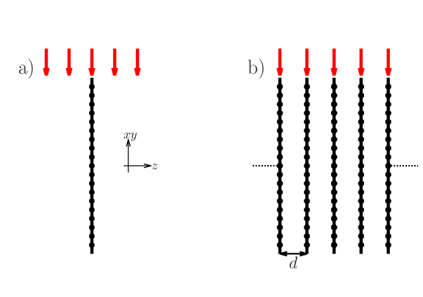
Our time-dependent density-functional theory (TDDFT) calculation of the permittivity consists of two steps. Since Q2D systems lack periodicity in the $z$-direction, it is customary to use the super-cell method [12, 13, 14]. First, in the super-cell geometry, we calculate the density-response function $\tilde{\chi}_{\mathbf{G}g,\mathbf{G}^{\prime}g^{\prime}}(\mathbf{q},\omega;d)$ of an auxiliary 3D system comprised of an infinite periodic array of monolayers with the separation $d$ between them, as is schematized in Fig. 1 b) (the dependence of $\tilde{\chi}$ on $d$ is shown explicitly). Here $g$ are reciprocal vectors in the $z$-direction.

We have conducted the calculation for the monolayer pristine graphene using the full-potential linear augmented plane-wave (FP-LAPW) code Elk [15]. The $z$-axis period $d$ of the super-cell was taken 20 a.u. The $k$-point grid of $512\times 512\times 1$, 30 empty bands, and the damping parameter of 0.002 a.u. were used in both the ground-state and the linear-response calculations. The former was carried out within the local-density approximation (LDA) [16] for the exchange-correlation (xc) potential, while the latter was the random-phase approximation (RPA) one (i.e., the xc kernel $f_{xc}$ [17] was set to zero).

Results for $\varepsilon_{\text{3D}}$, obtained through

are presented in the left panels of Figs. 2 and 3 for $q=0.049$ and $0.152$ a.u., respectively, along the $\Gamma M$ direction.

It is, however, known that $\varepsilon_{\text{3D}}(\mathbf{q},\omega;d)$, calculated in the super-cell geometry, is a quantity completely different from the permittivity $\varepsilon(\mathbf{q},\omega)$ of a single layer [12, 13, 14, 11], as can be also immediately appreciated from the $d$-dependence of the former. Our second step consists, therefore, in finding the density-response function $\chi$ of the single-layer system from that of the array of those layers $\tilde{\chi}$. This can be conveniently done by virtue of the matrix relation [11]

where the elements of the matrix $C$ are given by

In particular, $\chi$ calculated by Eqs. (3)-(4) is free of the spurious inter-layer interaction, which is present in $\tilde{\chi}$.

By the use of Eqs. (3)-(4), we find $\chi$ in the 3D reciprocal-space representation. Then, by the inverse Fourier transform to the mixed representation and using Eq. (1), we obtain the permittivity $\varepsilon(\mathbf{q},\omega)$. The latter is plotted in the right panels of Figs. 2 and 3.

A striking feature in Fig. 3, right panel, is that $\varepsilon(\mathbf{q},\omega=0)$ is negative and, since $\text{Im}\,\varepsilon(\mathbf{q},\omega\geq 0)\geq 0$, the permittivity of graphene does not satisfy Kramers-Kronig relations [2]

$\mathcal{P}$ denoting the principal value of the integrals, with $R(\omega)=\varepsilon(\mathbf{q},\omega)$. This fact is further illustrated in Fig. 4, where the real part of $\varepsilon(\mathbf{q},\omega)$ is compared with the KK transform of its imaginary part: The two functions coincide at $q<q_{c}$ (left panel), but they are largely different at $q>q_{c}$ (right panel). We found the critical wave-vector for graphene to be $q_{c}\approx 0.118$ a.u. ($0.223$ Å^-1). ¹¹ 1 Generally speaking, $q_{c}$ is different in different directions, however, it is practically isotropic in graphene. On the other hand, it can be seen in Figs. 2 and 3, left panels, that the array system has a positive static permittivity, which cannot be otherwise for a 3D periodic system within RPA [5].

Since KK relations are not satisfied by $\varepsilon(\mathbf{q},\omega)$, the latter must have a singularity in the complex $\omega$ upper half-plane. The singularity can only be a pole at $\omega=\omega_{s}$ satisfying

Considering that (a) $1/\varepsilon(\mathbf{q},\omega)$ is a real continuous function on the positive imaginary axis of the $\omega$-plane; (b) $1/\varepsilon(\mathbf{q},\omega=0)<0$ for $q>q_{c}$; and (c) $1/\varepsilon(\mathbf{q},\omega=i\infty)=1$, we conclude that, at $q>q_{c}$, there exists a point $\omega_{s}$ on the positive imaginary axis of the $\omega$-plane which satisfies Eq. (6). To find this point, we write by virtue of Cauchy’s integral formula

Expanding the complex inverse pemittivity in the right-hand side of Eq. (7) via its real and imaginary parts and using the parity properties of those functions, we can write

Further, the equality of the second term on the right-hand side to the third one can be easily proven with the use of the KK relations for $1/\varepsilon(\mathbf{q},\omega)$. We then have

We use Eq. (9) to calculate the inverse permittivity on the positive imaginary $\omega$-axis from our results for it on the real axis. In Fig. 5, this is plotted for the two wave-vectors, below and above the critical value.

Above the critical wave-vector, the inverse permittivity crosses zero (indicated by a circle in Fig. 5), which does not happen below the critical wave-vector. In Appendix A, we compare our results with the analytical ones known in the low-$q$ regime [19, 20].

We can gain a further insight into the situation using the approximate analytical relation between the Q2D permittivity of a single layer and the 3D permittivity of the array of those layers

rather than with the ’exact’ numerical solution of Eqs. (3)-(4). Equation (10), derived in Ref. 14, is a good approximation at $q$ far from the critical value from the both sides, as we demonstrate below in Fig. 7. Solving Eq. (10) with respect to $\varepsilon_{\text{3D}}$, we find that $1/\varepsilon$ is zero if

In Fig. 6, we plot $\varepsilon_{\text{3D}}(\mathbf{q},\omega;d)$ along the positive imaginary $\omega$. Although $\varepsilon_{\text{3D}}(\mathbf{q},\omega;d)$ is analytic in the upper complex $\omega$-plane at all values of $\mathbf{q}$, it gives rise to a zero in $1/\varepsilon$ (a pole in $\varepsilon$) when the condition (11) is met. In Fig. 6 this is shown as an intersection, in the case of $q>q_{c}$, with the straight horizontal line representing the right-hand side of Eq. (11).

Figure 7 is presented in support of the fact that the permittivity obtained through the ’exact’ numerical procedure via Eqs. (3), (4), and (1) can be accurately approximated by the simple analytical formula of Eq. (10), if $q$ is sufficiently below or above the critical wave-vector (upper panels). On the contrary, the same comparison done for the wave-vector slightly below and above the critical value (lower panels), reveals the complete inapplicability of the approximate formula (10) in the vicinity of the critical wave-vector. Moreover, a giant increase in the absolute value of the permittivity occurs close to the critical wave-vector.

Graphene is known to be a semi-metal, possessing a remarkable property of Dirac’s cones touching in the $K$-point of its band-structure [21]. A natural question arises whether the negative static permittivity and the violation of KK relations in graphene are in any way related to the Dirac’s cones in this material. To answer this, in Fig. 8 we present results for the permittivity of the hexagonal boron nitride ($h$-$\mathrm{BN}$), known to be an insulator [22]. Similar to graphene, above a critical wave-vector $q_{c}\approx 0.323$ a.u. ($0.610$ Å^-1) (right panel of Fig. 8), the permittivity of $\mathrm{BN}$ does not satisfy KK relations, while having a negative static limit. Furthermore, in Appendix B, we demonstrate that a simple local model of a metallic slab in vaccum supports the negative static permittivity at larger wave-vectors. This shows that the negative static permittivity and the breakdown of KK relations is a rather general property common to Q2D systems.

Importantly, in perfect 3D crystals the negative static permittivity is only possible due to the dynamic xc effects in the electronic response [5]. Since our results for Q2D crystals are obtained within the RPA, i.e., neglecting the xc effects, and the negative static permittivity occurs possible, the situation is fundamentally different with Q2D crystals: This is the finite but microscopic thickness of the crystal, which is also the break of the periodicity in one dimension, that makes the negative static permittivity possible. Nonetheless, static and dynamic many-body effects play an important part in Q2D crystals [23, 24], which have not been accounted for in the present study. In Appendix C, we show that the the inclusion of the xc kernel $f_{xc}$ on the level of the adiabatic time-dependent local-density approximation (ATDLDA) [25, 26, 17] does not lead to a significant change in the results. The inclusion of the same effects within TDDFT with more elaborate $f_{xc}$, e.g., following the schemes known in the 3D case [27, 28], presents a challenge in the case of Q2D systems. Furthermore, for Q2D crystals supported on substrates, the interaction with the latter strongly influences the excitation processes [29], which is also a demanding problem to be addressed in the future.

For the accurate interpretation of the results, it is necessary to keep in mind the exact meaning of the permittivity (1) of a Q2D crystal. This definition is given in two steps:[11] First, the 2D conductivity $\sigma^{\text{ext}}_{\text{2D}}$ with respect to the external field is introduced

where $\mathbf{E}^{\text{ext}}(\mathbf{q},\omega)$ is the uniform in the $z$-direction external electric field, and $\mathbf{j}_{\text{2D}}(\mathbf{q},\omega)$ is the 3D current-density integrated in the $z$-direction and averaged over the unit cell in the $xy$-plane. Secondly, the permittivity of a Q2D crystal is defined by the relation

rigorously valid for a strictly 2D system. The final justification of Eq. (13) is that with this definition the usual formula for the energy dissipation

holds for a Q2D crystal exactly. However, as detailed in Ref. 11, the Q2D permittivity cannot be attributed the meaning of the coefficient of proportionality between the external and the total fields and, hence, Eq. (14) cannot be rewritten in terms of $\mathbf{E}_{\text{tot}}$ and ${\rm Im}\,\varepsilon$. We note that these complications call for the particular caution in the consideration of the negative static permittivity in the context of the 2D superconductivity [4, 5]. The behavior of the total field along the $z$-direction in graphene is further discussed in Appendix Sec. D.

In conclusions, we have established the violation of Kramers-Kronig relations by the wave-vector and frequency dependent permittivity of quasi-two-dimensional graphene and boron nitride above a critical magnitude of the wave-vector, and the static permittivity was found negative in this case. The mechanism for the negative static permittivity was shown conceptually different from that in the 3D case: It is due to the system finite microscopic thickness rather than to the exchange-correlation effects. Our findings suggest the fundamental differences of the screening and the electronic excitation processes in quasi-2D crystals as compared with both 3D and purely 2D systems. It is, however, discussed that further work is required to consider the present results in the context of the 2D superconductivity.