A Metallicity Recipe for Rocky Planets
Abstract
Planets with sizes between those of Earth and Neptune divide into two populations: purely rocky bodies whose atmospheres contribute negligibly to their sizes, and larger gas-enveloped planets possessing voluminous and optically thick atmospheres. We show that whether a planet forms rocky or gas-enveloped depends on the solid surface density of its parent disk. Assembly times for rocky cores are sensitive to disk solid surface density. Lower surface densities spawn smaller planetary embryos; to assemble a core of given mass, smaller embryos require more mergers between bodies farther apart and therefore exponentially longer formation times. Gas accretion simulations yield a rule of thumb that a rocky core must be at least 2 before it can acquire a volumetrically significant atmosphere from its parent nebula. In disks of low solid surface density, cores of such mass appear only after the gas disk has dissipated, and so remain purely rocky. Higher surface density disks breed massive cores more quickly, within the gas disk lifetime, and so produce gas-enveloped planets. We test model predictions against observations, using planet radius as an observational proxy for gas-to-rock content and host star metallicity as a proxy for disk solid surface density. Theory can explain the observation that metal-rich stars host predominantly gas-enveloped planets.
Keywords:
planets and satellites: formation – planets and satellites: terrestrial planets – planets and satellites: dynamical evolution and stability1 Introduction
The Kepler Mission has discovered an abundance of planets — of order one per star (Fressin et al., 2013) — with orbital periods shorter than a year, and sizes smaller than that of Neptune (Borucki et al., 2011a; Borucki et al., 2011b; Batalha et al., 2013; Burke et al., 2014; Mullally et al., 2015). Kepler measurements of planet radii, when combined with planet masses measured via radial-velocity follow-up (Marcy et al., 2014; Weiss & Marcy, 2014; Dressing & Charbonneau, 2015) and transit timing variations (Ford et al., 2011; Fabrycky et al., 2012; Ford et al., 2012a; Ford et al., 2012b; Lithwick, Xie & Wu, 2012; Steffen et al., 2012b; Steffen et al., 2012a; Mazeh et al., 2013; Steffen et al., 2013; Wu & Lithwick, 2013; Hadden & Lithwick, 2014; Xie, 2014), reveal a surprising diversity of bulk densities. Some planets are dense enough to be made practically exclusively of solid refractory elements — e.g., Kepler-10b (Batalha et al., 2011) and Kepler-36b (Carter et al., 2012) — whereas others require voluminous volatile components, e.g., the Kepler-11 planets (Lissauer et al., 2011; Lissauer et al., 2013) and Kepler-36c (Carter et al., 2012). We refer to the former class as “purely rocky” (a.k.a. “super-Earths”) and the latter as “gas-enveloped” (a.k.a. “mini-Neptunes”).
Purely rocky planets can undergo transformation to gas-enveloped, and vice versa, through a variety of physical processes including outgassing (Rogers et al., 2011), photoevaporation (Lopez, Fortney & Miller, 2012; Lopez & Fortney, 2013), and collisional stripping of atmospheres (Schlichting, Sari & Yalinewich, 2015). Our interest here is in determining a planet’s make-up just after its formation. We seek to identify the factors that dictate whether or not a rocky core can accrete a volumetrically significant atmosphere from its parent nebula (Lee, Chiang & Ormel, 2014). We highlight the decisive role played by the surface density of solids in the primordial disk — and by extension the host star metallicity — in controlling how long a rocky core takes to coagulate. According to our interpretation, purely rocky planets are born within disks of low solid surface density and accordingly have long gestation times: they attain core masses large enough to acquire atmospheres only after their ambient gas disks have dissipated. Recent breakthroughs linking planet radius to composition (Lopez & Fortney, 2014; Rogers, 2015) allow us to identify with confidence purely rocky vs. gas-enveloped planets in the Kepler sample for comparison with theoretical models.
We present a planet formation scenario in Section 2, deriving approximate analytic estimates for the masses of the seed bodies or “embryos” that merge to form super-Earths and the underlying cores of mini-Neptunes, and the ambient gas densities during the merger era. These order-of-magnitude considerations set the stage for numerical simulations in Section 3, where we combine -body integrations with atmospheric accretion models to show that disks with the highest solid surface densities spawn gas-enveloped planets, whereas disks having sufficiently low solid surface densities produce purely rocky planets. In Section 4, we translate, as best we can, model predictions for gas mass fraction vs. disk surface density into the observables of planet radius vs. host star metallicity. There we compare to the observed sample of Kepler candidates with spectroscopic host star metallicities (Buchhave et al., 2014) and find support for the link between disk surface density and small planets’ composition. We conclude in Section 5.
2 Overview of formation scenario and initial conditions
The solids in a protoplanetary disk provide the raw material for building rocky planets and the cores of gas-enveloped planets. Planetesimals may have either formed in situ or accumulated by radial drift from larger orbital distances.
In a disk of solid surface density , an “embryo” (a.k.a. isolation mass) consumes all the solids within its feeding zone of annular width :
| (1) |
To give a sense of scale, if , where
| (2) |
is the mutual Hill radius and is the host star’s mass, then is approximately the mass of Mars at semi-major axis 0.3 AU in a disk with (for context, this surface density is about 3 that of the solid component of the minimum-mass solar nebula; see, e.g., Chiang & Youdin 2010 and use their ). We will consider other possibilities for and below.
At short orbital periods, isolation-mass embryos grow quickly, consuming the planetesimals in their annuli well before the gas disk dissipates. The growth or coagulation timescale is approximately
| (3) |
where is the orbital frequency, the embryo’s density, the embryo’s radius, and is the enhancement of the growth rate due to gravitational focusing (e.g., Goldreich, Lithwick & Sari 2004). For example, even without gravitational focusing (), the Mars-mass embryo mentioned above takes only 0.2 Myr to grow.
2.1 Embryo self-stirring as the gas disk dissipates
While the gas disk is still present, it damps the embryos’ eccentricities by dynamical friction, preventing them from crossing orbits, merging, and growing to larger masses. The gas disk needs to dissipate so that the embryos’ self-stirring becomes more effective against dynamical friction. The goal of this subsection is to gauge the degree of gas depletion, and the magnitudes of the embryos’ random velocities and spacings, at the time that embryos cross orbits — i.e., at the onset of the “giant impact” stage of planet formation. This will inform the choice of initial conditions for the -body coagulation simulations in Section 3 --- which will not include gas dynamical friction. 11 1 Our analysis in Section 2 assumes that embryos do not open gaps in the gas disk. Whether this is true depends on the disk viscosity (e.g., Duffell 2015, and references therein). Gaps weaken eccentricity damping by gas, but open the possibility of eccentricity excitation by gas (Goldreich & Sari, 2003). In any case, we do not expect gaps to seriously interfere with the ability of rocky cores to accrete gas envelopes, since the gas accretion rate is insensitive to the ambient gas density (Lee, Chiang & Ormel, 2014) and since gas in the gap is continuously replenished by viscous radial inflow (Lubow & D’Angelo, 2006).
We sketch below the various regimes for the embryos’ equilibrium random velocities . There are three velocity scales. The Hill velocity, , tends to be the smallest:
The sound speed, , is not much larger. We assume a disk temperature of
| (5) |
yielding a sound speed
| (6) |
where is the Boltzmann constant and g is the mean molecular mass.
The largest scale is the escape velocity from the surface of the embryo:
2.1.1 Growth of random velocities to
During the first stage of stirring, the embryos’ random velocities are below . Their stirring rate is
| (8) |
(Goldreich, Lithwick & Sari, 2004). At the same time, gas damps random velocities at a rate
| (9) |
(Kominami & Ida, 2002, e.g.,), resulting in an equilibrium,
The embryos’ random velocities grow to once the gas surface density drops to
This condition evaluates to for Mars-mass embryos at , or for Earth-mass embryos at 1 AU. For disks initialized with cosmic gas-to-solid ratios of , little or no depletion is required for .
2.1.2 Growth of random velocities to
Next the big bodies stir each other from random velocities of to . The gas damping rate remains the same (Equation 9), but the stirring rate decreases to
| (10) |
(Goldreich, Lithwick & Sari, 2004), resulting in a new equilibrium
Random velocities reach once .
2.1.3 Growth of random velocities to
Once the gas density drops enough for to exceed , the gas damping rate decreases to the classical formula for dynamical friction (Papaloizou & Larwood, 2000). We assume the random energy is equipartitioned so that the random vertical velocity is and the embryo remains marginally embedded in gas. The new damping rate is
and the random velocity reaches a new equilibrium of
until .
2.1.4 Gas damping shuts off
Finally, once so that , the embryo is no longer embedded in the disk but plunges through the disk twice per orbit, reducing the gas damping further to
| (12) |
(Ford & Chiang, 2007; Rein, 2012). At this stage, stirring (Equation 10) always exceeds gas dynamical friction; gas damping effectively shuts off and cannot establish a velocity equilibrium.
2.1.5 The case of widely spaced embryos
The stirring rates cited above (Equations 8 and 10) are based on the particle-in-a-box approximation, which holds only for embryos spaced closely enough (Ford & Chiang, 2007). Spacings widen as embryos merge, eventually invalidating the approximation. We estimate the reduced stirring rate by using the encounter map of Hasegawa & Nakazawa (1990). Two planets separated in semimajor axis by undergo close encounters every synodic period . Each encounter increases planetary eccentricities by as given by
| (13) |
(Hasegawa & Nakazawa 1990, their equation 38). The stirring rate is then
| (14) |
Substituting
| (15) |
yields
| (16) |
This formula is probably an upper limit to the true stirring rate, as it assumes that the planets’ eccentricity and inclination vectors are randomized between encounters (i.e., Equation 13 is “phase-averaged”).
For , equating Equation 16 to the damping rate in Equation 9 results in a velocity equilibrium
| (17) |
The equilibrium velocity reaches when the gas surface density drops to
| (18) |
This condition evaluates to for Mars-mass embryos at 0.3 AU separated by .
Once the equilibrium velocity exceeds , the ratio of the stirring rate (Equation 16) to the damping rate (Equation 11) grows with , and the velocity equilibrium is no longer stable. In this case, gas damping shuts off. However, it may not stay shut off. Equation 18 suggests that as embryos grow more widely spaced through successive mergers, eccentricity damping by gas may return to significance, bringing the equilibrium velocity back below and necessitating further reductions in to effect more mergers. For example, Equation 18 evaluates to for cores separated by 10 at 0.3 AU. Intermittent gas damping would both increase the total core growth timescale and limit the amount of gas a planet can ultimately accrete. We will not account for such ongoing gas damping in the remainder of the paper, but a detailed, self-consistent treatment for parameters appropriate to close-in super-Earths is an important subject for future work (see, e.g., Kominami & Ida 2002 for a study pertinent to solar system terrestrial planets).
2.2 Growth to super-Earths and mini-Neptunes in the giant impact stage
The results of the previous section suggest that, as a rough rule of thumb, is the condition that deactivates gas dynamical friction and that triggers when embryos can cross orbits and merge; furthermore, at the start of this giant impact stage, random velocities . An alternative scaling for the random velocity is to use ; Ida & Makino (1993) find that Hill scalings are appropriate for mutual stirring of oligarchs in the presence of planetesimals (neglecting gas). We will experiment with both scalings, respectively, in sections 2.2.1 and 2.2.2.
With , the giant impact stage commences with ample gas for merging embryos to accrete. How much gas the growing rocky cores actually accrete depends on how long the merging process takes. If a super-Earth-mass core takes too long to coagulate, the already depleted gaseous nebula will have completely dissipated (by viscous accretion onto the star) before the core can acquire a volumetrically significant atmosphere.
The timescale for embryos to cross orbits is (Yoshinaga, Kokubo & Makino, 1999):
| (19) |
where and are constants that depend on the initial random velocities — in units of — and is the number of mutual Hill radii between embryos. Therefore for a given set of embryo separations and initial velocities scaled by their Hill values, the timescale for the first merger is independent of . But for the small values of in low disks, one merger is not enough to build super-Earth cores; the timescale to grow to depends strongly on , as we now show.
2.2.1 Initial conditions set by the Hill scale
We start by considering the case where the initial , , and are independent of . For example, Hansen & Murray (2012) and Hansen & Murray (2013) recently simulated the giant impact stage with initial orbital spacings defined using a fixed multiple of , and random velocities independent of . In this set up, the first orbit crossing time is independent of . However, the number of mergers will depend on . For an initial spacing of Hill radii, the embryo mass (Equation 1) is
| (20) |
where (Kokubo & Ida, 2002, e.g.,).
To grow to — here loosely defined as the minimum mass necessary to accrete a volumetrically significant atmosphere — equal-mass embryos must undergo approximately mergers, each of which increases the number of Hill spacings by (since each merger increases the absolute separation between embryos by a factor of 2 while the mutual Hill radius increases by a factor of ). The timescale for the final merger to form is therefore
which we can rewrite as
where is independent of . Therefore the time to form depends exponentially on the solid surface density.
2.2.2 Initial conditions set by gas sound speed
If the initial spacings and random velocities are scaled instead by the gas sound speed (sections 2.1.2–2.1.4), then
and
The timescale for the final merger is
The coefficient may also depend on , because does not scale with . Yoshinaga, Kokubo & Makino (1999) found that , where . Then for ,
where and are independent of . Alternatively, if initial random velocities are damped to zero by mergers that precede the final doubling, then
Either way, we see that the final merger to reach takes a time that is exponentially sensitive to .
3 Simulations of core growth and gas accretion
We saw in Section 2 that embryos begin crossing orbits and merging when the gas surface density drops below the solid surface density . The subsequent merger history unfolds over a timescale that is exponentially sensitive to . High disks promise to spawn massive cores quickly enough that they can accrete volumetrically significant atmospheres before the gas disk dissipates. Here we determine using -body coagulation simulations whether this promise can be fulfilled.
3.1 -body simulations of core growth

We run four sets of -body integrations using mercury6 (Chambers, 1999) to simulate the era of giant impacts, similar to those run by Chambers & Wetherill (1998) and Hansen & Murray (2012); Hansen & Murray (2013). We use the hybrid symplectic integrator with a time step of 0.5 days and a close encounter distance (which triggers a transition from the symplectic integrator to the Burlisch-Stoer integrator) of 1 . In each set of 500 integrations, we begin with isolation-mass embryos resulting from disk solid surface densities spanning 3–400 g/cm2 at 1 AU (). All surface density profiles scale as .
In the first set of simulations (corresponding to the scaling arguments in Section 2.2.1), the embryo masses are defined by annuli each spanning 10 mutual Hill radii , similar to Hansen & Murray (2012); Hansen & Murray (2013) and Kokubo & Ida (1998); Kokubo & Ida (2002). The embryos’ initial semi-major axes span . Initial random velocities are set to the Hill velocity , equipartitioned between eccentricity () and inclination (). In the second set of simulations (corresponding to Section 2.2.2), the embryo masses are defined by annuli spanning , and random velocities are set to (Equation 6), similarly equipartitioned. In these first and second sets of simulations, all bodies have bulk densities set to 1 g/cm3, which defines their collisional cross-sections. The third and fourth set of simulations correspond to the first and second sets, respectively, except with bulk densities of 5 g/cm3 instead of 1 g/cm3. (For comparison, Hansen & Murray (2013) use 3 g/cm3.) Because the results did not change materially upon using the higher bulk density, all of the results shown below will be drawn from our first and second simulation sets.
The solid surface density, by means of setting the initial embryo masses, strongly affects the core coagulation timescale. Smaller initial embryos necessitate more mergers to reach a given core mass. More mergers take longer time (exponentially longer, according to the rough arguments presented in Section 2). In Figure 1, we show example snapshots from three simulations (all with Hill-scaled initial conditions) of disks with different . Cores quickly reach substantial masses in the highest disk; take millions of years to form in a lower disk; and remain low mass in the lowest disk. Next we summarize the results of two sets of 500 simulations a piece. In Figures 2 and 3, we plot the time to grow to , as a function of , for four sample values of . Figure 2 corresponds to Hill-scaled initial conditions and Figure 3 to those set by . A horizontal dashed line marks an approximate remaining lifetime of 1 Myr for the gas disk once has declined to . We employ only those simulations for which the maximum core mass attained is less than 30 Earth masses. For a wide range of , the embryos can grow to in sufficiently short time to accrete atmospheres and become enveloped by gas; in some cases, the embryo mass itself exceeds (gray regions). But for a subset of lower disks, the time to grow to is much longer than the remaining gas disk lifetime; such planets run out of time to accrete gas and remain purely rocky.


3.2 Atmospheric accretion models
Lee, Chiang & Ormel (2014) computed how a rocky core of a given mass accretes gas from the primordial nebula, with specific application to Kepler planets. We use their model to generate, for an array of core masses, a set of gas accretion histories that we will combine in Section 3.3 with the -body coagulation simulations from Section 3.1. This combination will enable us to determine, for any given protoplanet, the simultaneous time evolution of core mass and atmospheric mass fraction GCR gas-to-core mass ratio.
For each core mass , we run the Lee, Chiang & Ormel (2014) model for two nebular temperatures K appropriate for two orbital distances , respectively. For every and , we adopt two nebular gas densities. The higher gas density is chosen such that , where is that (extreme) value required to form as an isolation-mass embryo from a --wide annulus at the given . The lower gas density is this value. The set of models so constructed span a large enough range of and that they can be usefully interpolated. We run one set of gas accretion simulations using solar metallicity opacities with dust, and another set of 16 simulations using solar metallicity opacities without dust (for technical details, see Lee, Chiang & Ormel 2014 and Ferguson et al. 2005). Model parameters are summarized in Table 1, including the corresponding values of .
[b] (AU) (K) ( g/cm3) 0.7 600 1 65 41 0.65 2 100 64 1.0 4 160 102 1.6 10 300 188 3 0.3 900 1 1000 62 10a 2 1600 98 16 4 2600 156 26 10 4700 287 47
- a
The {1 , 0.3 AU, low } model could not be evolved because its outer radiative zone was too thin to be resolved. The omission of this model is unimportant because we do not expect it to yield a volumetrically significant atmosphere, judging from our other 1- models.
Figure 4 plots the resulting gas accretion histories for dusty-atmosphere opacities. As discussed by Lee, Chiang & Ormel (2014), these histories are not very sensitive to outer boundary conditions like , , or , because accretion is controlled by the ability of the atmosphere to cool internally, i.e., by conditions at the atmosphere’s radiative-convective boundary which is largely decoupled from the nebula. From Figure 4 we infer the following rule of thumb: a core must be at least 2 to accrete a volumetrically significant atmosphere within 1 Myr. (A gas depletion timescale shorter than 1 Myr would correspond to a larger core mass for the rule of thumb.) For example, a 2 core located at 0.3 AU within a disk having g/cm3 accretes a GCR 1% atmosphere within 1 Myr. If said core has an Earth-like composition, corresponding to a radius of 1.2 , a 1% atmosphere would inflate the planet’s total radius to 2 (Lopez & Fortney, 2014). For context, core masses also avoid complete atmospheric loss by photoevaporation at –1 AU, assuming a 10% efficiency in converting incident XUV radiation from the host star into the kinetic energy of a planetary outflow (Figure 2 of Lopez & Fortney 2013; see also Owen & Wu 2013).

3.3 Combining core growth and atmospheric accretion
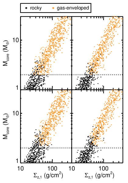
We now use the results from the atmospheric accretion simulations (Figure 4) to identify which of the cores grown in the -body simulations (Figures 2 and 3) acquire voluminous gas envelopes vs. stay purely rocky. We carry out two methods of analysis. The first and simpler procedure is to apply the rule of thumb described in Section 3.2. We declare that all cores that grow to 2 within 1 Myr accrete a gas envelope, and that all cores that fail to grow that quickly remain rocky. We plot the results of this experiment in the top panels of Figure 5 for both our Hill-scaled and sound-speed-scaled coagulation simulations. We see that only disks with higher solid surface densities — g/cm2 — always spawn cores fast enough to pick up atmospheres.
The results of a second, more detailed procedure are shown in the bottom panels of Figure 5. Here each core is prescribed to accrete an atmosphere based on the evolutionary tracks shown in Figure 4. By interpolating these tracks, we infer a gas-to-core mass fraction, , where .22 2 Technically because isolation-mass embryos can accrete gas before the giant impact era begins. In practice, because the gas accretion rate depends so steeply on core mass (see Figure 4), this initial amount of gas acquired is negligible compared to that accreted later when the core mass is larger. Let be the array of merger times for a given core. For simplicity and because the dependence of the accretion rate on the gas density is weak, we assume that the gas disk (which has already been depleted to based on the considerations in Section 2) remains in place for 1 Myr (the results are not sensitive to this exact time) and disappears thereafter:
If the first merger Myr, the final atmospheric gas content of the planet equals . Otherwise we interpolate the evolutionary tracks to calculate just before the first merger. Just after the first merger, we assume that, because of atmospheric loss from the giant impact, the new body starts with half the GCR of the larger merging body.33 3 In practice, this atmospheric loss is not important because gas accretion occurring after the last merger prior to the disappearance of the gas disk typically dominates. This is meant to be an approximation to the more realistic treatments developed by Schlichting, Sari & Yalinewich (2015) and Inamdar & Schlichting (2015). Note that the overwhelming majority of mergers are between bodies of comparable mass. From there, the GCR follows a new track appropriate to its new , accreting additional gas for . This process repeats until Myr. See Figure 4 for an example evolutionary trajectory.
Planets that attain GCR are considered gas-enveloped and colored orange in Figures 5 and 6. This second method yields essentially identical results to the first rule-of-thumb treatment.
In all panels of Figure 5, we see that the lowest disks produce predominantly rocky (black) planets; intermediate disks yield a combination of gas-free and gas-enveloped (orange) planets; and the highest disks spawn exclusively gas-enveloped planets. Figure 5 indicates that virtually all planets with final masses above 5 accrete gaseous envelopes, suggesting that radial-velocity discoveries like GJ 876 e (a 12.5 planet with a 124-day orbital period; Rivera et al. 2010) or 61 Vir c (a 10.6 planet with a 38-day orbital period; Vogt et al. 2010) are mini-Neptunes rather than super-Earths.
Inamdar & Schlichting (2015) also recently simulated the atmospheric mass fractions attained by an ensemble of planets that grow from isolation mass to core mass during the giant impact stage. Their isolation masses are formed from annuli wide and having a solid surface density such that observed exoplanets of mass can form from feeding zones that are wide, where is evaluated for (Schlichting, 2014). They simulate the accretion of gas during the isolation mass stage; subsequent atmospheric loss during giant impacts; and the final post-giant impact accretion of gas. The giant impacts are based on Monte Carlo simulations — by comparison with the -body simulations presented here — and atmospheric loss is treated in a more detailed and realistic way than our simple factor-of-2 prescription. When they consider only atmospheres accreted during the isolation-mass stage and subsequently eroded through impacts, the resulting atmospheric masses fractions are low, on the order of 10-3 (their Figure 8). However, atmospheric mass fractions reach several percent for subsequent accretion by core masses above beyond 0.15 AU (their Figure 9), unless the energy from giant impacts happens to be released over exactly the disk dissipation timescale. Thus our results are consistent with their post-giant impact results, in which gas accretion is dominated by the largest core mass achieved before the dissipation of the gas disk.
3.4 Effects of migration
The formation theory we have explored above is an in-situ theory; the planets are assumed to form in place. We sketch here how our results are impacted by orbital migration. Transporting bodies by gravitational torques in a disk (for a review, see Kley & Nelson 2012) can: (1) supply planetary embryos from the outer disk to the inner disk; (2) establish a resonant chain of protoplanets in the inner disk (but see Goldreich & Schlichting 2014 for reasons to believe such resonant locks are easily broken); and (3) move fully formed super-Earths and mini-Neptunes to the inner disk. We will argue that all these effects are compatible with our thesis that the disk’s solid surface density is a major determinant in a planet’s final gas-to-rock ratio.
In scenario (1), planet formation would proceed as detailed above (Sections 3.1–3.3) but with reflecting the surface density of embryos supplied from the outer disk rather than the surface density of dust/planetesimals in the inner disk. The simulations of Sections 3.1–3.3 model events post-dating the growth or delivery of embryos, so migration scenario (1) would not impact our conclusions qualitatively. Scenario (2) would be characterized by larger orbital spacings between protocores and longer orbit crossing times. Nevertheless the de-stabilization time should depend on planet masses (see, e.g., the resonant chains exhibited by the inner moons of Uranus; French, Dawson & Showalter 2015) which in turn would reflect the isolation masses in the outer disk; thus merger times should still depend sensitively on . Finally, under scenario (3), coagulation of rocky cores and accretion of gas would occur at larger orbital distances, where isolation masses are larger and orbital timescales are longer. The latter two effects appear to cancel for our fiducial semi-major axis range (0.04–1 AU); the black vs. blue points in Figures 2 and 3 exhibit similar trends. Whether they cancel so nearly at larger semi-major axes remains to be determined. If they do not cancel, then the threshold required to produce gas-enveloped planets could be larger or smaller, but it would still exist; i.e., we would still expect a population of purely rocky planets in the lowest disks. Because feeding zone annuli tend to be wider at larger orbital distances, cores formed in the outer disk do not need as large a to produce cores that are massive enough to accrete significant amounts of gas as isolation masses.
Recent models incorporating the effects of migration have assessed the effect of a parameter analogous to on the properties of super-Earths and mini-Neptunes. Cossou et al. (2014) simulated planet formation with -body integrations combined with prescriptive migration maps. Not treating gas accretion by cores, they found that disks with a higher mass in embryos delivered more massive super-Earth cores to the inner disk. We would expect these more massive cores to more easily acquire atmospheres (Section 3.2). In addition, Ida & Lin (2010) found that, for a range of migration speeds, the typical mass of super-Earths that migrate to AU increases with disk solid surface density normalization. The delivery of higher-mass planets to the interior regions of disks with overall higher solid density is consistent with our statement that the masses of planets that arrived by migration reflect the isolation masses in the outer disk.
4 Comparison to the Kepler sample
We argued above that the disk’s solid surface density is critical for determining whether a planet forms rocky or gas-enveloped. Here we translate the results from Section 3 — compositions as a function of — into observables to compare with the large Kepler sample of super-Earths and mini-Neptunes.
4.1 Observational proxies
Kepler has discovered about 3000 planet candidates with sizes between that of Earth and Neptune. Statistical modeling of the potential astrophysical false positive population has revealed that less than 10% of the candidates are false positives (Morton & Johnson, 2011; Fressin et al., 2013), allowing us to treat the sample as representative of true planets. Most Kepler candidates have measured radii but unknown masses. Lopez & Fortney (2014) recently argued that a planet’s radius can serve as a proxy for its composition (i.e., gas-to-rock content), assuming an envelope composed of hydrogen, helium, and an admixture of metals.44 4 In many models, the atmospheric metallicity can be as large as . In particular, planets larger than require a gas-to-core mass fraction exceeding 1%. This prediction has been borne out by the Kepler data. From a statistical analysis of planets with measured masses and radii, Rogers (2015) (see also Weiss & Marcy 2014 and Wolfgang & Lopez 2015) found that the cut-off radius between planets dense enough to be rocky and those requiring a significant volatile component sits at 1.6; a planet of radius has a 50% probability of being purely rocky. Between 1.5 to 2 , planets appear to transition from being purely rocky to having volumetrically significant gas envelopes (Figure 5 of Rogers 2015). A similar transition is suggested by planets with orbital periods shorter than 1 day — a.k.a. ultra-short period planets or USPs. Because USPs are so intensely irradiated by their host stars, they may have lost their primordial atmospheres to photoevaporation and may therefore exhibit a radius distribution corresponding to that of purely rocky cores. All the USPs studied by Sanchis-Ojeda et al. (2014) have radii , consistent with the interpretation that planets with larger radii possess voluminous gaseous envelopes.
Together, these recent advances allow us to identify Kepler planets as rocky or gas-enveloped based on their radii alone. We pay particular attention below to Kepler planets with periods longer than 15 days, since photoevaporation can remove the envelopes of shorter period planets (e.g., Lopez & Fortney 2013), leaving behind a planet that is purely rocky by nurture rather than by nature.
Having opted for planet radius as a proxy for composition, we now need a proxy for . Motivated by the strong correlation between giant planet occurrence and host star metallicity (Santos, Israelian & Mayor, 2001; Fischer & Valenti, 2005; Buchhave et al., 2012; Buchhave et al., 2014; Wang & Fischer, 2015), we use the spectroscopic of planet-hosting stars as a proxy for the surface density of their primordial planet-forming disks. Kepler follow-up teams have observed stellar spectra for hundreds of KOI (Kepler Object of Interest) host stars. Buchhave et al. (2014) recently published a catalogue of measured using the stellar parameter classification (SPC) tool developed by Buchhave et al. (2012). Because the host stars span a narrow stellar mass range, while spans nearly a full dex, we expect that should track — or at least its value averaged over the entire disk (it may not track the local value of because solids can concentrate radially in disks, so that the local disk metallicity can deviate from the bulk stellar metallicity — more on this point in Section 4.3). Buchhave et al. (2014) reported that hosts of KOIs with 2–4 have higher metallicities than hosts of smaller KOIs. Schlaufman (2015) recently argued against the statistical significance of this finding.

4.2 A metallicity divide for rocky planets
In Figure 6, we plot the results of the simulations from Section 3 with the added dimension of orbital period. The transition that divides gas-enveloped planets (orange points) from purely rocky planets (black points) decreases slightly with orbital period. Longer orbital periods correspond to larger isolation masses, lowering the threshold to spawn gas-enveloped planets only. This effect may be related to the observed rise in the occurrence rate of Neptune-sized planets at longer orbital periods (Dong & Zhu, 2013), though the concomitant weakening of photoevaporation at large orbital distances likely also contributes. (See also Figure 7 of Foreman-Mackey, Hogg & Morton 2014.) Regardless, beyond 20 days, the transition flattens to about 40 g/cm2, about 2 the lowest that can spawn close-in planets more massive than Earth, or about 4 the value of the minimum-mass solar nebula. Note that near this transition , a mixture of gas-enveloped and purely rocky planets is produced.

Next we plot, in Figure 7, the observed host star metal fraction (relative to solar) vs. orbital period using the Buchhave et al. (2014) catalogue of stars with spectroscopic parameters. We use radius as a proxy for composition, color-coding orange those planets with radii exceeding 2 to signify that they likely have volumetrically significant atmospheres. We remove KOIs designated as false positives in the NExSci database (Mullally et al., 2015). Figure 7 attests that at orbital periods days, beyond the reach of photoevaporation, metal-rich stars (in the pink box) lack rocky planets, whereas lower metallicity stars (in the gray box) host a mixture of rocky and gas-enveloped planets. This trend is related to that reported by Buchhave et al. (2014), who found that planets above 1.7 Earth radii orbit higher metallicity stars. Instead of identifying a cut in planet radius, we identify a cut in metallicity above which stars host exclusively gas-enveloped, not rocky, planets. Unlike the simulations shown in Figure 6, the observations shown in Figure 7 show no evidence that only rocky planets orbit the lowest metallicity stars; we will expand upon this point in Section 4.3 (see Figure 8).
We compute a K-S statistic comparing the distributions of planetary radii in the pink vs. gray boxes in Figure 7, yielding a formal statistical probability of 0.00045 that the difference in the distribution of radii is due to chance. It is not clear theoretically what the exact value of the metallicity divide should be between the pink and gray boxes; the existence of a metallicity divide is physically motivated by Sections 2–3 which highlight the role played by the solid surface density in determining a planet’s final gas content, but the exact mapping between and is not known. Despite this uncertainty, the high (formal) statistical confidence reflected in the K-S test is robust against a range of values for . In the Appendix, we perform an alternative statistical test that accounts for our freedom in choosing ; we find there that a model with a metallicity divide is preferred to one without at 95% confidence. The period cut of 15 days delineating the left boundaries of the pink and gray boxes is motivated by considerations of photoevaporation; for example, photoevaporation has been invoked to explain the rocky composition of Kepler-36b, which has a 13.8 day orbital period (Lopez & Fortney, 2013).
In interpreting the observations, we have assumed that the reported metallicities are correct relative to one another. Figure 7 should be remade if improved stellar parameters are obtained. For example, if the stars reported as metal-rich were actually giant stars, it would not have been possible to detect small planets orbiting them, and their identification as planet-hosting stars would be incorrect. Another potential complication is that stars more rich in metals tend to be larger than their metal-poor counterparts, making it more difficult to detect smaller (rocky) planets orbiting the former. In the sample here, the average size of stars that have metallicities and that host a 1–4 KOI with a period days is . By comparison, for stars with , the average size is . Nevertheless, the stellar radius ranges of the two samples have substantial overlap, and the difference in the median stellar projected areas implies only a 20% difference in signal-to-noise for transit detections. We also tried restricting the sample to stars for which otherwise identical planets of could have been detected; this reduced the sample size but did not change the results qualitatively. Therefore we interpret the trend identified in Figure 7 to be real and not just a selection effect, but we recommend revisiting the trend as the sample size of spectroscopically measured KOI hosts grows. We also recommend the publication of the joint two-dimensional posteriors for stellar metallicity and stellar radius so that any covariance in the inferred parameters can be accommodated.

4.3 Planet radius vs. host star metallicity in detail
We can add another layer of modeling by computing precise planetary radii from our simulations. The interior structure models of Lopez & Fortney (2013) yield an empirical formula for planetary radius as a function of core mass and GCR. Planet radii so evaluated using the simulation data from Section 3 are plotted against in Figure 8, and compared alongside the observed distribution of planet radii vs. host star metallicity. In both simulations and observations we see an “empty wedge” at large (large host star metallicity) and small planetary radius.
However, Figure 8 also reveals a discrepancy with the observations. The simulations predict a second empty wedge: an absence of large radius planets in the lowest disks. But this region of parameter space is actually populated by the observations55 5 Schlaufman (2015) found a linear correlation between planet radius and host star metallicity using a collection of candidates with sizes extending to 15 ; that trend may be dominated by planets larger than 4 so we do not compare here.. There are a few possible explanations. First, may be an imperfect proxy for . Some disks orbiting metal-poor stars may have disproportionately large if the solids in their primordial disks drifted radially inward by aerodynamic drag and accumulated at small orbital distances (e.g., Youdin & Shu 2002; Youdin & Chiang 2004; Chiang & Youdin 2010; Hansen & Murray 2012; Chatterjee & Tan 2014). In other words, the disk’s solids-to-gas ratio at any particular location can differ from the stellar metallicity because solids and gas can segregate in disks (see also Andrews et al. 2012). Second, gas-enveloped planets may have formed at larger separations beyond 1 AU — where isolation masses are larger — and migrated in (see Section 3.4).
5 Conclusions
Kepler has discovered an abundance of planets with voluminous atmospheres. A small mass percentage of volatiles — 1% for typical mini-Neptunes (e.g., Wolfgang & Lopez 2015) — can dramatically inflate a planet’s radius beyond that of its rocky core, with significant consequences for surface temperature, pressure, and habitability. Gas-enveloped planets are the rule around stars with supersolar metallicities; atmosphere-laden planets are also found orbiting stars with subsolar metallicities, together with purely rocky planets having practically no contribution to their radii from their atmospheres.
What determines whether a rocky core acquires an atmosphere or not? We have found that the protoplanetary disk’s surface density in solids is a key ingredient in recipes for forming rocky vs. gas-enveloped planets. In Section 2 we used order-of-magnitude scaling relations to show that low solid surface densities prolong the timescale for a core to grow from embryos, so much so that by the time the core is massive enough to acquire an atmosphere, there may not be any disk gas left. Long coagulation timescales in low solid surface density disks are a consequence of the larger number of mergers required to assemble a core from smaller isolation-mass embryos. In Section 3, we combined -body simulations of core assembly with one-dimensional gas accretion models to show that the highest surface density disks produce primarily gas-enveloped planets, whereas lower solid surface density disks can produce both gas-enveloped and rocky planets. In Section 4, using the Buchhave et al. (2014) spectroscopic sample, we presented observational evidence for a lack of purely rocky planets orbiting metal-rich stars at orbital periods 15 days (Figure 7 and left panel of Figure 8). This trend is another manifestation of the correlation between planet radius and host star metallicity for small planets reported previously (Buchhave et al., 2014; Wang & Fischer, 2015). If we assume a 1-to-1 correlation between host star metallicity and disk solid surface density, then we can reproduce the absence of purely rocky planets around metal-rich stars (i.e., high solid surface density disks; Figure 8). But this same simple model does not reproduce the observation that metal-poor stars also host gas-enveloped planets with sizes up to 4 Earth radii (Figure 8). This probably means that the assumption of a 1-to-1 correlation between stellar metallicity and disk surface density is inadequate; radial drift and accumulation of solids (for a review, see Chiang & Youdin 2010) can yield high surface density disks (and therefore gas-enveloped planets) even around stars with low bulk metallicity. Alternatively, it might also be that the in-situ planet formation models used here, which have a hard time producing “super-puffy” planets with low core masses and extended atmospheres (Masuda, 2014, e.g.,), need to account for migration. As argued in Section 3.4, migration should produce qualitatively similar trends in planet composition vs. disk solid surface density. The subset of mini-Neptunes orbiting metal-poor stars may have migrated from afar, where isolation masses are larger.
These results may bear on other recently discovered trends between host star metallicity and the properties of small planets. Adibekyan et al. (2013, their Figure 1) found that low-mass planets ) orbiting metal-rich stars have orbital periods shorter than 20 days, whereas more massive planets, and planets orbiting metal-poor stars, span a range of orbital periods. The restriction of mini-Neptunes/super-Earths to short orbital periods around metal-rich stars may be a manifestation of how embryo masses — and presumably final core masses — increase with increasing orbital distance. That is, at large orbital distances in a high surface density disk, embryo masses may be so large that the disk cannot help but spawn high-mass planets. Relatedly, Beaugé & Nesvorný (2013, their Figure 6) found that super-Earths and mini-Neptunes (radii ) hosted by low-metallicity stars have orbital periods greater than 5 days; that super-Earths and mini-Neptunes with orbital periods shorter than 5 days are hosted by high-metallicity stars; and that metal-poor stars do not harbor planets with radii . Their reported trends — which may stem from the higher solid surface densities expected to accompany higher metallicity stars, in concert with the rise in embryo mass with orbital period — could be revisited with the latest sample of spectroscopic metallicities from Buchhave et al. (2014).
We have assumed in this paper that mini-Neptunes are either purely rocky or gas-enveloped. The possibility that mini-Neptunes are “water-worlds” having a large fraction of their mass in water or ices cannot be discounted based on mass and radius measurements alone (see, e.g., the case of GJ 1214b; Rogers & Seager 2010). Our study favors the interpretation that mini-Neptunes are gas-enveloped and not water-worlds; we would not expect the prevalence of purely rocky vs. icy planets to be a strong function of disk solid surface density or host star metallicity.
Our study supports the idea that the volatiles in mini-Neptunes are directly accreted from the primordial nebula rather than outgassed from rock, as outgassing does not obviously lead to the observed trends with stellar metallicity / disk solid surface density. Further evidence for nebular accretion can be found in the ultra-short period ( day) planets studied by Sanchis-Ojeda et al. (2014). These have a radius cut-off of 1.7 — consistent with the transition from rocky to gas-enveloped planets (Rogers, 2015), but below the 3 break above which the planet occurrence rate decreases at larger orbital distances (Petigura, Marcy & Howard, 2013). The absence of planets with voluminous gas envelopes at the shortest orbital periods is more consistent with nebular accretion: at these close-in distances, primordially accreted atmospheres are readily lost to photoevaporation during the first 0.1 Gyr of the host star’s evolution (e.g., Owen & Wu 2013), whereas steam or gradually outgassed atmospheres can be maintained or replenished throughout the star’s lifetime. The one notable exception of a non-rocky ultra-short period planet is 55 Cnc e, which has an orbital period of 0.74 days (Dawson & Fabrycky, 2010), a radius of 2 , and a density too low to be purely rocky (Winn et al., 2011). Intriguingly, it is situated in a system with two close-in giant planets whose proximity to a mean-motion resonance (Marcy et al., 2002; McArthur et al., 2004; Fischer et al., 2008) suggests they underwent orbital migration. Thus 55 Cnc e may also have been transported from afar; it may be one of an uncommon class of migrated icy planets, interloping among the majority of super-Earths and mini-Neptunes that coagulated and acquired their atmospheres in situ.
Acknowledgments
We are grateful to the referee for a useful report. We thank Hilke Schlichting for several particularly helpful and insightful discussions. We also appreciate valuable exchanges with Lars Buchhave, Jonathan Fortney, Brad Hansen, Jack Lissauer, Eric Lopez, Geoff Marcy, Sean Raymond, Leslie Rogers, Kevin Schlaufman, Scott Tremaine, and Angie Wolfgang. RID gratefully acknowledges funding by the Berkeley Miller Institute for Basic Research in Science. EC acknowledges support from grants AST-0909210 and AST-1411954 awarded by the National Science Foundation, NASA Origins grant NNX13AI57G, and Hubble Space Telescope grant HST-AR-12823.001-A. EJL is supported in part by the Natural Sciences and Engineering Research Council of Canada under PGS D3 and the Berkeley Fellowship. Some of this research was conducted at the Kavli Institute for Theoretical Physics program on the Dynamics and Evolution of Earth-like Planets, supported in part by the National Science Foundation under Grant No. NSF PHY11-25915.
This paper makes use of the extremely valuable collection of planets discovered by the Kepler Mission. Funding for the Kepler mission is provided by the NASA Science Mission Directorate. We are grateful to the Kepler team for all their work on this revolutionizing mission and to the ground-based follow-up teams for their host star characterization. This research has made use of the NASA Exoplanet Archive, which is operated by the California Institute of Technology, under contract with the National Aeronautics and Space Administration under the Exoplanet Exploration Program. The simulations presented here were run on the SAVIO computational cluster resource provided by the Berkeley Research Computing program at the University of California Berkeley, supported by the UC Chancellor, the UC Berkeley Vice Chancellor of Research, and the Office of the Chief Information Officer.
References
- Adibekyan et al. (2013) Adibekyan V. Z. et al., 2013, A&A, 560, A51
- Andrews et al. (2012) Andrews S. M. et al., 2012, ApJ, 744, 162
- Batalha et al. (2011) Batalha N. M. et al., 2011, ApJ, 729, 27
- Batalha et al. (2013) Batalha N. M. et al., 2013, ApJS, 204, 24
- Beaugé & Nesvorný (2013) Beaugé C., Nesvorný D., 2013, ApJ, 763, 12
- Borucki et al. (2011a) Borucki W. J. et al., 2011a, ApJ, 728, 117
- Borucki et al. (2011b) Borucki W. J. et al., 2011b, ApJ, 736, 19
- Buchhave et al. (2014) Buchhave L. A. et al., 2014, Nature, 509, 593
- Buchhave et al. (2012) Buchhave L. A. et al., 2012, Nature, 486, 375
- Burke et al. (2014) Burke C. J. et al., 2014, ApJS, 210, 19
- Carter et al. (2012) Carter J. A. et al., 2012, Science, 337, 556
- Chambers (1999) Chambers J. E., 1999, MNRAS, 304, 793
- Chambers & Wetherill (1998) Chambers J. E., Wetherill G. W., 1998, Icarus, 136, 304
- Chatterjee & Tan (2014) Chatterjee S., Tan J. C., 2014, ApJ, 780, 53
- Chiang & Youdin (2010) Chiang E., Youdin A. N., 2010, Annual Review of Earth and Planetary Sciences, 38, 493
- Cossou et al. (2014) Cossou C., Raymond S. N., Hersant F., Pierens A., 2014, A&A, 569, A56
- Dawson & Fabrycky (2010) Dawson R. I., Fabrycky D. C., 2010, ApJ, 722, 937
- Dong & Zhu (2013) Dong S., Zhu Z., 2013, ApJ, 778, 53
- Dressing & Charbonneau (2015) Dressing C. D., Charbonneau D., 2015, ApJ, 807, 45
- Duffell (2015) Duffell P. C., 2015, ApJ, 807, L11
- Fabrycky et al. (2012) Fabrycky D. C. et al., 2012, ApJ, 750, 114
- Ferguson et al. (2005) Ferguson J. W., Alexander D. R., Allard F., Barman T., Bodnarik J. G., Hauschildt P. H., Heffner-Wong A., Tamanai A., 2005, ApJ, 623, 585
- Fischer et al. (2008) Fischer D. A. et al., 2008, ApJ, 675, 790
- Fischer & Valenti (2005) Fischer D. A., Valenti J., 2005, ApJ, 622, 1102
- Ford & Chiang (2007) Ford E. B., Chiang E. I., 2007, ApJ, 661, 602
- Ford et al. (2012a) Ford E. B. et al., 2012a, ApJ, 750, 113
- Ford et al. (2012b) Ford E. B. et al., 2012b, ApJ, 756, 185
- Ford et al. (2011) Ford E. B. et al., 2011, ApJS, 197, 2
- Foreman-Mackey, Hogg & Morton (2014) Foreman-Mackey D., Hogg D. W., Morton T. D., 2014, ApJ, 795, 64
- French, Dawson & Showalter (2015) French R. G., Dawson R. I., Showalter M. R., 2015, AJ, 149, 142
- Fressin et al. (2013) Fressin F. et al., 2013, ApJ, 766, 81
- Goldreich, Lithwick & Sari (2004) Goldreich P., Lithwick Y., Sari R., 2004, ARA&A, 42, 549
- Goldreich & Sari (2003) Goldreich P., Sari R., 2003, ApJ, 585, 1024
- Goldreich & Schlichting (2014) Goldreich P., Schlichting H. E., 2014, AJ, 147, 32
- Hadden & Lithwick (2014) Hadden S., Lithwick Y., 2014, ApJ, 787, 80
- Hansen & Murray (2012) Hansen B. M. S., Murray N., 2012, ApJ, 751, 158
- Hansen & Murray (2013) Hansen B. M. S., Murray N., 2013, ApJ, 775, 53
- Hasegawa & Nakazawa (1990) Hasegawa M., Nakazawa K., 1990, A&A, 227, 619
- Ida & Lin (2010) Ida S., Lin D. N. C., 2010, ApJ, 719, 810
- Ida & Makino (1993) Ida S., Makino J., 1993, Icarus, 106, 210
- Inamdar & Schlichting (2015) Inamdar N. K., Schlichting H. E., 2015, MNRAS, 448, 1751
- Kley & Nelson (2012) Kley W., Nelson R. P., 2012, ARA&A, 50, 211
- Kokubo & Ida (1998) Kokubo E., Ida S., 1998, Icarus, 131, 171
- Kokubo & Ida (2002) Kokubo E., Ida S., 2002, ApJ, 581, 666
- Kominami & Ida (2002) Kominami J., Ida S., 2002, Icarus, 157, 43
- Lee, Chiang & Ormel (2014) Lee E. J., Chiang E., Ormel C. W., 2014, ApJ, 797, 95
- Lissauer et al. (2011) Lissauer J. J. et al., 2011, Nature, 470, 53
- Lissauer et al. (2013) Lissauer J. J. et al., 2013, ApJ, 770, 131
- Lithwick, Xie & Wu (2012) Lithwick Y., Xie J., Wu Y., 2012, ApJ, 761, 122
- Lopez & Fortney (2013) Lopez E. D., Fortney J. J., 2013, ApJ, 776, 2
- Lopez & Fortney (2014) Lopez E. D., Fortney J. J., 2014, ApJ, 792, 1
- Lopez, Fortney & Miller (2012) Lopez E. D., Fortney J. J., Miller N., 2012, ApJ, 761, 59
- Lubow & D’Angelo (2006) Lubow S. H., D’Angelo G., 2006, ApJ, 641, 526
- Marcy et al. (2002) Marcy G. W., Butler R. P., Fischer D. A., Laughlin G., Vogt S. S., Henry G. W., Pourbaix D., 2002, ApJ, 581, 1375
- Marcy et al. (2014) Marcy G. W. et al., 2014, ApJS, 210, 20
- Masuda (2014) Masuda K., 2014, ApJ, 783, 53
- Mazeh et al. (2013) Mazeh T. et al., 2013, ApJS, 208, 16
- McArthur et al. (2004) McArthur B. E. et al., 2004, ApJ, 614, L81
- Morton & Johnson (2011) Morton T. D., Johnson J. A., 2011, ApJ, 738, 170
- Mullally et al. (2015) Mullally F. et al., 2015, ApJS, 217, 31
- Owen & Wu (2013) Owen J. E., Wu Y., 2013, ApJ, 775, 105
- Papaloizou & Larwood (2000) Papaloizou J. C. B., Larwood J. D., 2000, MNRAS, 315, 823
- Petigura, Marcy & Howard (2013) Petigura E. A., Marcy G. W., Howard A. W., 2013, ApJ, 770, 69
- Rein (2012) Rein H., 2012, MNRAS, 422, 3611
- Rivera et al. (2010) Rivera E. J., Laughlin G., Butler R. P., Vogt S. S., Haghighipour N., Meschiari S., 2010, ApJ, 719, 890
- Rogers (2015) Rogers L. A., 2015, ApJ, 801, 41
- Rogers et al. (2011) Rogers L. A., Bodenheimer P., Lissauer J. J., Seager S., 2011, ApJ, 738, 59
- Rogers & Seager (2010) Rogers L. A., Seager S., 2010, ApJ, 716, 1208
- Sanchis-Ojeda et al. (2014) Sanchis-Ojeda R., Rappaport S., Winn J. N., Kotson M. C., Levine A., El Mellah I., 2014, ApJ, 787, 47
- Santos, Israelian & Mayor (2001) Santos N. C., Israelian G., Mayor M., 2001, A&A, 373, 1019
- Schlaufman (2015) Schlaufman K. C., 2015, ApJ, 799, L26
- Schlichting (2014) Schlichting H. E., 2014, ApJ, 795, L15
- Schlichting, Sari & Yalinewich (2015) Schlichting H. E., Sari R., Yalinewich A., 2015, Icarus, 247, 81
- Steffen et al. (2013) Steffen J. H. et al., 2013, MNRAS, 428, 1077
- Steffen et al. (2012a) Steffen J. H. et al., 2012a, MNRAS, 421, 2342
- Steffen et al. (2012b) Steffen J. H. et al., 2012b, ApJ, 756, 186
- Vogt et al. (2010) Vogt S. S. et al., 2010, ApJ, 708, 1366
- Wang & Fischer (2015) Wang J., Fischer D. A., 2015, AJ, 149, 14
- Weiss & Marcy (2014) Weiss L. M., Marcy G. W., 2014, ApJ, 783, L6
- Winn et al. (2011) Winn J. N. et al., 2011, ApJ, 737, L18
- Wolfgang & Lopez (2015) Wolfgang A., Lopez E., 2015, ApJ, 806, 183
- Wu & Lithwick (2013) Wu Y., Lithwick Y., 2013, ApJ, 772, 74
- Xie (2014) Xie J.-W., 2014, ApJS, 210, 25
- Yoshinaga, Kokubo & Makino (1999) Yoshinaga K., Kokubo E., Makino J., 1999, Icarus, 139, 328
- Youdin & Chiang (2004) Youdin A. N., Chiang E. I., 2004, ApJ, 601, 1109
- Youdin & Shu (2002) Youdin A. N., Shu F. H., 2002, ApJ, 580, 494
Appendix A Statistical significance of absence of rocky planets orbiting metal-rich stars
As an alternative statistical test that accounts for our freedom in choosing the metallicity divide, we compute an odds ratio to compare a model with a metallicity divide (model 1) to one without (model 2). For the former, we marginalize over the metallicity divide. The odds ratio of model 1 over model 2 is:
| (21) |
If we give equal prior weight to the two models, the odds ratio becomes:
| (22) |
Here the data are the inferred compositions of observed planets, so we define a probability that an observed planet is rocky, , given its observed radius and uncertainty . The uncertainty is assumed to define a normal distribution and is computed by propagating the uncertainty from the stellar radius (Buchhave et al., 2014) and transit depth (Mullally et al., 2015), assuming that the uncertainties in these quantities are independent. For simplicity, we estimate
We clarify that this differs from the defined by Rogers (2015), who compute based on both mass and radius measurements. Our abstracts the results of Rogers (2015) and other studies (Lopez & Fortney, 2014; Sanchis-Ojeda et al., 2014; Weiss & Marcy, 2014; Wolfgang & Lopez, 2015) to assert that is an approximate cut-off above which a planet is very unlikely to be purely rocky. We marginalize over the uncertainty in the planet’s radius:
| (24) |
Next we evaluate the denominator of the odds ratio in Equation 22, the probability of the data given the model without the metallicity divide (model 2):
| (25) |
where refers to an individual planet. Equation 25 marginalizes over , the fraction of the sample comprised of rocky planets (e.g., for an even mixture of rocky and gaseous planets).
A similar formula to Equation 25 yields the probability of the data given model 1 for host stars with metallicities below the divide ; now is the fraction of the sample below the divide that is rocky:
| (26) |
By contrast, above , planets are unlikely to be rocky. We marginalize over , the fraction of the sample above the cut that is rocky, assuming ranges from 0 to 10%:
| (27) |
Marginalizing over , we have
| (28) |