UT–15–20
TU–997
August 24, 2026
Strong IR Cancellation in Heavy Quarkonium
and Precise Top Mass Determination
Y. Kiyoa,
G. Mishimab and
Y. Suminoc
a Department of Physics, Juntendo University
Inzai, Chiba 270-1695, Japan
b Department of Physics, University of Tokyo
Bunkyo-ku, Tokyo 113-0033, Japan
c Department of Physics, Tohoku University
Sendai, 980-8578 Japan
Combining recent perturbative analyses on the static QCD potential and the quark pole mass, we find that, for the heavy quarkonium states , and , (1) ultra-soft (US) corrections in the binding energies are small, and (2) there is a stronger cancellation of IR contributions than what has been predicted by renormalon dominance hypothesis. By contrast, for a hypothetical heavy quarkonium system with a small number of active quark flavors (), we observe evidence that renormalon dominance holds accurately and that non-negligible contributions from US corrections exist. In addition, we examine contributions of renormalons at . As an important consequence, we improve on a previous prediction for possible achievable accuracy of top quark –mass measurement at a future linear collider and estimate that in principle 20–30 MeV accuracy is reachable.
During the past few decades, there have been significant developments in the analysis of heavy quarkonium systems using perturbative QCD. Developments in computational technology greatly advanced our understanding on the nature of quark masses and interquark forces. We anticipate that eventually these developments will deepen our understanding on the structure of perturbative QCD in more general contexts.
Recently an important step toward this direction has been achieved. A computation was completed of the four-loop relation between the quark pole mass and the mass in the modified-minimal-subtraction scheme ( mass) [1]. This result, when combined with other known results such as the three-loop correction () to the static QCD potential [2], sets our analysis at a new stage, namely, at full next-to-next-to-next-to-leading order (NNNLO) in terms of short-distance quark masses. It realizes a cancellation of infra-red (IR) dynamics at this order.
In this first analysis we report what can be learned by combining existing results. In particular we compare the results of [3, 4, 1] to make clearer the nature of the perturbative series of the heavy quarkonium energies, concerning (1) corrections from the ultra-soft (US) energy scale and (2) the renormalon dominance hypothesis. In addition, we examine contributions of an ultra-violet (UV) renormalon at and discuss possible contributions of an IR renormalon at .
Motivations for performing such an analysis can be stated as follows. A few years ago, a convincing evidence has been presented for the existence of IR renormalons in the perturbative series of the energy of a static color source, which has an IR structure common to the quark pole mass [5]. Hence, it is among general interests how accurately the renormalon dominance picture holds for the quark pole mass. Furthermore, contributions of US corrections to the quarkonium energy have collected attention since long time [6, 7, 8]. Despite an original expectation of being dominating at IR, there have been evidences that US corrections are moderate in size from comparisons of the perturbative predictions with experimental data for the bottomonium spectrum [9, 10], phenomenological potential models of heavy quarkonia [11], and lattice computations of [12]. However, extraction of an accurate size of the US corrections still remains a challenge [13].
Important applications of this type of analysis include precise determination of the masses of the heavy quarks , and from the energy levels of the lowest-lying heavy quarkonium states [14]. (For earlier works, see [15] and references therein.) In this paper we apply our new understanding to a study of the possible achievable accuracy of top quark mass measurement expected at a future linear collider. Today, a precise determination of the top quark mass is highly demanded, for a precision test of the standard model of particle physics (SM) [16], and also since the top quark mass plays a crucial role in the vacuum stability of the SM at a very high energy scale [17]. Hence, progress in our understanding of the heavy quarkonium states may lead to an access to deep aspects of the SM.
The pole- mass relation can be expressed in a series expansion in the strong coupling constant as
| (1) |
Here, denotes the mass renormalized at the mass scale; represents the strong coupling constant in the scheme, where is the number of massless quark flavors (, 4 and 5 for the charm, bottom and top quarks, respectively); the renormalization scale is set to . In most part of this paper, we use the coupling constant of the theory with flavors only as the expansion parameter. The coefficients can be obtained from the corresponding mass relations in the full theory (with heavy quarks and light quarks), respectively, by rewriting them in terms of the coupling constant of the theory with light quarks only.
Let us first summarize the results of the previous analyses, on which our analysis is based. Refs. [3, 4] estimated on the basis of different assumptions, prior to Ref. [1], which accomplished the exact computation of :
- •
Ref. [3] required stability of the perturbative prediction for at relatively large . Essentially the only assumption made is that US corrections in do not deteriorate perturbative stability (which holds up to NNLO) at NNNLO.
- •
Ref. [4] assumed renormalon dominance in and and estimated their contributions from the latter. Contribution of US corrections in was subtracted in this estimate.** * Since US corrections in do not contribute to the renormalon at , this manipulation is justified within the renormalon dominance hypothesis.
- •
| 0 | 1 | 2 | 3 | 4 | 5 | 6 | |
|---|---|---|---|---|---|---|---|
Only the values for are presented explicitly in the final form in [1] (for the full theory with ). Since we need the values for other ’s in our analysis, we derive the exact result of given as a cubic polynomial of as
| (2) |
where an error of is assigned to its value for each . We determined the last two coefficients of eq. (2) by a fit using the results of [18, 19] in addition to the result of [1]. For the reader’s convenience, we list the exact result of in the full theory in Tab. 1 using this formula for .
As already mentioned, we convert the above formula using the coupling of the theory with massless quarks only as the expansion parameter. This gives
| (3) |
with the same error . In the rest of the analysis, we use this for various ’s.
In Tab. 2 we summarize the two estimates and the exact result for .†† † Since we use the converted , its values for listed in this table are different from TABLE III of [1]. In this sense, the comparison in TABLE III of [1] is not consistent, since ’s in the different definitions are compared. Numerically the differences due to different definitions are small, nonetheless. The relative accuracies are compared visually in Fig. 1. Overall, we find a reasonable agreement of the previous estimates and the exact results, with respect to the assigned errors. The relative accuracies of the estimates are also fairly good, at order 10% level. These features provide certain justification to the used assumptions in these estimates.
| 0 | 1 | 2 | 3 | 4 | 5 | 6 | |
|---|---|---|---|---|---|---|---|
| [3] | — | — | 1668(167) | — | |||
| [4] | 2887(133) | 2291(98) | 1772(82) | 1324(81) | 945(92) | 629(191) | |
| [1] | 2848.4(21.5) | 2228.4(21.5) | 1687.1(21.5) | 1220.3(21.5) | 824.1(21.5) | 494.3(21.5) |
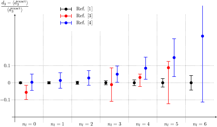
Furthermore, we can make a closer examination. In particular, the central (optimal) values of in the table and figure carry important information on the respective assumptions. We should note that the errors of are only systematic and have no statistical nature. Hence, by carefully contemplating on the origins of these systematic errors, we can extract the sizes and signs of the systematic effects. The agreement with respect to the systematic errors is a necessary condition for the validity of our analysis given below.
In the cases , corresponding to , , quarkonium states, respectively, we see a good agreement of the estimates by [3] with the exact values, whereas the estimates by [4] are slightly larger. On the other hand, for smaller , which correspond to hypothetical heavy quarkonium systems, the agreement between the estimates by [4] and the exact results is fairly good, whereas the estimate by [3] for is slightly smaller than the exact value. From these observations we derive the following interpretation:
- •
For , (i) US corrections in are small, and (ii) there is a stronger cancellation of IR contributions than what has been predicted by renormalon dominance hypothesis.
- •
For , (iii) renormalon dominance holds more accurately, and (iv) non-negligible contributions from US corrections exist.
We explain the details in the following.
The renormalon dominance hypothesis assumes that the expansion coefficient of the perturbative series is dominated by a factorial () growth [20],
| (4) |
which stems from the singularity at in the Borel transform of the perturbative series. [ , and denotes the -loop coefficient of the beta function of . ] Contributions from the analytic part at are neglected. The comparison between and the central values of shows that the renormalon dominance hypothesis works better for smaller . This suggests that the above factorial growth overwhelms contributions from the analytic part as becomes larger for smaller .
Another source of dependence of the renormalon dominance resides in the series [20, 22]
| (5) |
in eq. (33) of [4]. The factor multiplies the right-hand side of eq. (4), giving suppressed corrections, so that it shows how the expansion coefficient approaches the asymptotic form at large orders ().‡‡ ‡ Contributions from the analytic part at are not included in the series , as they are suppressed exponentially. Fig. 2 plots the series (5) in our case for different ’s. They exhibit the tendency that suppressed contributions become more important for larger , although the first term (=1) is by far dominating. Both of these dependences in analytic and suppressed contributions have been taken into account in the error estimates of [4]. The former error enters as scale dependences in the analysis of [4] and is the main source of errors.

One may wonder if the UV renormalon at contained in the pole mass gives a significant contribution to the perturbative series of the pole mass. Based on an analysis in the large- approximation, we estimate that the contribution of the renormalon to is fairly small compared to the errors of [4] listed in Tab. 2. This is consistent, since the analytic part at contributes dominantly to these errors, and the renormalon belongs to the analytic part. The analysis also suggests that the renormalon contribution is not a dominant component of the analytic part. Another important feature is that, since the UV renormalon is Borel summable and gives a well-defined contribution, as long as we obtain a converging series of a physical observable (such as the heavy quarkonium energy level), the contribution of the renormalon to the error estimate becomes small (arbitrarily small unlike IR renormalons). Indeed contribution to the error is minor at our present perturbative order. We give details of the analysis of the UV renormalon in the Appendix.
Similarly there may be effects by the IR renormalon contained in the pole mass, whose properties are less known. Known properties are as follows [21]. (a) It is induced by the non-relativistic kinetic energy operator ; (b) It is not forbidden by any symmetry, and parametrically it possibly induces an order uncertainty; (c) It does not appear in the large- approximation. With this limited knowledge, it is not easy to estimate contribution of the renormalon in the estimate of in [4]. In principle, this contribution is exponentially suppressed in the estimate of the renormalon in the pole mass and is encoded in the scale dependence in the error estimate of .
We turn to the estimates of by [3], which incorporate the fact that cancellation of IR dynamics occurs beyond the renormalon dominance hypothesis. It can be understood using the potential-NRQCD effective field theory [8], in which interactions of a heavy quarkonium and IR degrees of freedom are systematically organized in multipole expansion in . The leading order interaction is given by the interaction of an IR gluon with the total color charge of the heavy quarkonium, which vanishes for a color-singlet system. The corresponding contribution to the binding energy is given by an -independent IR part of [23]. The cancellation between and is not restricted to the renormalon part, and the analytic part at contains such contributions.
In this general framework, the lowest order non-canceled IR contribution to the energy is given by a double insertion of the dipole interaction between the color-electric field and heavy quarkonium, expressed in terms of a non-local gluon condensate of the form . It is dominated by contributions from the US energy scale, and the perturbative evaluation of this condensate at and has been incorporated in in the estimate of . In principle, the renormalon in the pole mass (if it exists) can affect . However, the large mass limit is taken in the analysis of [3], so that the renormalon (order ) is suppressed compared to the renormalon (order ). Hence, the estimate of should not be affected by the renormalon. Furthermore, in estimating the effects of taking the large mass limit are small for , compared to the real , , -quark mass cases, hence, our discussion is expected to be valid for these real heavy quarkonium systems. In the cases and , perturbative analysis makes sense only in a hypothetical static limit , and our discussion is confined to this limit.
In perturbative QCD, instability against scale variation in IR region is manifest for all the physical observables, reflecting the blow-up of the running coupling constant at IR. For a “good” observable, generally scale dependence decreases as the order of perturbative expansion is raised. Empirically this happens not only in the ultra-violet (UV) direction but also stability extends to IR region as the perturbation order is increased. In the case of the heavy quarkonium energy, the leading source of IR instability is the non-local gluon condensate dominated by US corrections. The (optimal) values of the estimates of in the first line of Tab. 2 are chosen to optimize the stability of the perturbative prediction for the energy in the IR region at NNNLO. A very good coincidence of these values with the exact results for suggests that the US corrections are small for these systems. Here, we may set the criterion for “large” or “small” by whether the corrections deteriorate stability of the perturbative prediction or not.
As shown in [3], perturbative stability of is sensitive to the precise value of , and this sensitivity turns out to be asymmetric with respect to the sign of a variation of .§§ § Qualitatively the same feature is observed for the heavy quarkonium energy levels [24]. If is larger than a certain critical value, stability of the prediction is lost very quickly. This leads to a fairly sharp upper bound on the estimate of for each . By contrast, stability of the prediction is degraded only gradually if is lowered from its optimal value. In this regard, a marked result is that in the case the exact value of is on the verge of or slightly above the upper bound of required by stability of the energy. Since US corrections are expected to be the source of IR instability of the energy, we infer that the US corrections are sizable in this case. Oppositely, in the case , the exact value of lies slightly below that required by optimal stability of the energy. Hence, in this case US corrections do not deteriorate perturbative stability in any essential way, and US corrections may well be regarded as “small.” Such a dependence of IR stability on may result from the fact that the running coupling constant blows up most rapidly for , while the running becomes milder as increases. (Note that we consider massless quarks.) If an IR catastrophe of perturbative stability should ever occur, it would be expected to appear first in the most rapidly running case. To demonstrate explicitly the level of instability in the case , we show a plot according to the analysis of [3]. Fig. 3 shows the scale dependences of at a relatively large , where perturbative stability up to NNLO is close to marginal. The NNNLO line is flatter than the NNLO line in the large region, however, it grows in the small region and starts to show a sign of instability. See [3] for more details of the analysis method.

There is a difficulty in quantifying the size of US corrections more directly. By definition, the US corrections are dependent on the factorization scale , which should satisfy the condition [8]
| (6) |
where is the Casimir operator for the adjoint representation. Given the different dependences of and , we confirm that a simple logarithmic dependence of the US corrections on , proportional to , cannot explain the difference, even if we assume a reasonable dependence of . This is expected, since except in dimensional regularization, which conceals power-like dependences on the scales, we expect a much stronger dependence of the US corrections. This dependence should eventually turn into a dependence on the physical US scales, namely should be replaced by and , where presumably the latter is more dominant at larger .¶¶ ¶ dependence is canceled in physical observables. Hence, we are ultimately interested in the dependence of physical observables on the physical US scale. At lower orders of perturbative series, only the scale is visible. As the order is raised, perturbative expansion becomes more sensitive to the scale. The leading dependence of on should appear as . This requires (at least) an analysis analogous to that of [4] incorporating the singularity in addition. Furthermore, we would need to separate UV and IR contributions in perturbative expansion systematically, to be able to accurately extract the US contributions [25, 26]. Such a detailed analysis is beyond the scope of this paper.
Thus, for the case , we are (for the time being) content with the observation that everything is consistent. The renormalon dominance hypothesis can accurately estimate by the method of [4]. As mentioned, it is plausible that the renormalon dominance works most accurately in this case.** * This feature appears to be slightly reinforced for by a cancellation of the contribution from the UV renormalon and other contributions from the analytic part at ; compare Tabs. 2 and 3. On the other hand, stability of at IR can in principle be jeopardized by US corrections and, if at all, this is expected to happen for smaller .
In contrast, for , the analytic part at has a larger relative significance, and the central values of the estimates by [4] depart from the exact values; see Tab. 2 and Fig. 1. We can circumvent this problem in the method of [3], since cancellation of IR dynamics takes place in the analytic part as well, and the contribution of US corrections is expected to be milder than the case. Thus, we are led to the interpretation as presented in the beginning of this discussion.
On the basis of our understanding up to this point, we reexamine the prediction of the energy level of the (would-be) toponium state, using the NNNLO formula for the energy level [27, 28, 29]. We compare with the analysis [30], which examined the energy level calculated in terms of and in the expansion [31]. The large- approximation (a crude approximation based on renormalon dominance) was used for estimates of and .†† † More accurately, a Padé estimate of was used and the prediction of the energy level was shown to be quite close to that of the large- approximation. Since the difference is minor and irrelevant in our context, we refer only to the large- approximation. We replace them by the exact values. The essence of the analysis [30] is to use the renormalon dominance hypothesis for estimating a perturbative error in the top quark mass determination from the energy level of the toponium state. As a result, about 40 MeV for an expected accuracy was predicted for determination of the top quark mass.

All the qualitative argument of [30] based on renormalon dominance hypothesis should be valid, since, as we have verified, the renormalon dominance is qualitatively a good approximation. Nevertheless, according to our above understanding, the accuracy of the prediction is expected to improve, since the cancellation of IR dynamics occurs at a deeper level than that of the large- approximation. In the system, the leading non-canceled IR contribution from US corrections is expected to be “small” if our understanding is consistent.
Fig. 4 compares the scale dependence of the toponium energy by the previous analysis [30] and that using the exact values of and . A marked difference is that the former prediction is much more unstable in the IR region than the latter. This is consistent with our expectation. There also appears a flat region (minimal-sensitivity scale [32]) in the new prediction, which is absent in the former prediction.
We estimate the error of the new prediction. It is natural to use the scale dependence around the minimal-sensitivity scale ( GeV).‡‡ ‡ From the general argument based on the renormalon dominance hypothesis, the minimal-sensitivity scale is expected to increase as the perturbation order is raised [25]; see Fig. 6. Following the standard prescription we vary the scale by factors 1/2 and 2. When the scale is varied between 80 and 320 GeV, the energy varies by about 20 MeV below and above the minimal-sensitivity scale, respectively. Therefore, the sum of the absolute variations of the energy level is about 40 MeV.§§ § This is a factor 2 more conservative estimate than taking the maximal variation of the energy level in this range. The corresponding variation of the top quark mass is almost one half of it, leading to about 20 MeV, which we take as an error estimate. Another error estimate may be obtained from the difference between the NNLO prediction at the minimal sensitivity scale (at NNLO) and that at NNNLO, namely the difference between the values of at the local maxima at NNLO and NNNLO in Fig. 6. This gives 30 MeV as an uncertainty for the top quark mass. For reference, we show the series expansion in at the minimal sensitivity scale at NNNLO:
| (7) |
which shows a healthy convergence behavior [ GeV and ]. Thus, we estimate an error in the top quark mass determination from to be 20–30 MeV.
We note that the naive error estimate of order by the uncanceled renormalon at in [30] is order 3–10 MeV, which is still somewhat smaller than the current error estimate. This means that the current perturbative order would not be high enough to be limited by this renormalon uncertainty. Contribution of the renormalon at in the pole mass is estimated to be a few MeV or less (see the Appendix), while contribution of the renormalon is estimated naively to be order – MeV (corresponding to – MeV).
In Ref. [30] the range of the scale variation was taken differently from the above range, since no minimal-sensitivity scale for the energy exists for that prediction and a different criterion was used. We may check consistency. If we vary the scale in the above range for the previous prediction, we obtain the same error estimate for the top quark mass as in [30] (about 40 MeV).
Thus, we obtained a better possible accuracy of the top quark mass determination at a future linear collider over the previous estimate, which relied only on the renormalon dominance hypothesis before the full computations of and . We consider that it is not a sheer numerical accident but with a reasoning that we obtain a smaller error estimate. Namely, from the general property of QCD a stronger IR cancellation than what is predicted by the renormalon dominance hypothesis follows. This interpretation is supported by a detailed comparison between the estimates of for from stability of and the estimates by the renormalon dominance, and also by an overall consistent picture drawn in the first part of this paper.


To clarify the current status, we show in Fig. 6 dependences of the energy level on the current uncertainty of the exact value of and on the input value of [33]. The former induces about 10 MeV variation (5 MeV for the top quark mass) at the minimal-sensitivity scale, while the latter induces about 90 MeV (45 MeV for the top mass) variation. Hence, a precise determination of , of the order of accuracy, is prerequisite to achieve 20–30 MeV accuracy of the top quark mass determination. Prediction of with higher precision is also favorable.
For comparison, we perform a similar analysis using the potential subtracted (PS) mass [34] as the input parameter. (The definition of the NNNLO PS mass is given in [27].) Fig. 6 shows the scale dependence of the toponium energy level, where we use the PS mass . To compare with the mass, we vary the scale from to and find the variation of the energy level of about . (For , the variation is about , which is consistent with [35].) The uncertainty of causes shift of the NNNLO energy level.¶¶ ¶ The dependence of the PS mass on starts from the order , which is the reason for a smaller dependence compared to the mass. Thus, use of the PS mass leads to a larger scale variation of the perturbative prediction for the energy level than the mass. We observe qualitatively different scale dependences between the two schemes by comparing Figs. 6 and 6, where this tendency is apparent not only at NNNLO but also at lower orders. Furthermore, we confirm a similar tendency in the scale dependences for other ’s, where the values of vary considerably. We also note that the conversion formula between the PS and masses induces a scale uncertainty of order 30 MeV for provided that GeV is an input value.
Intuitively the difference between using the and PS masses may be understood as follows. In the –mass scheme, the energy of the toponium bound state consists of (i) the masses of and , (ii) contributions to the self-energies of and not renormalized into the mass (typically from gluons whose wavelengths are larger than the Compton wavelength of , ), and (iii) the potential energy between and . IR contributions between (ii) and (iii) (typically from larger than the bound-state size) get canceled, where the domain of IR cancellation is determined dynamically by the wave function of the bound state [9, 36, 26].
The composition of the energy of the bound state in the PS–mass scheme is similar, except that the renormalized mass (i) is replaced by the PS mass, which renormalizes the top quark self-energy from . In the computation of the self-energy, a sharp cut-off is introduced in momentum space at the factorization scale , which is chosen to be of the order of the Bohr scale . The cut-off induces a power dependence of the PS mass on . Since the is close to the bound-state size, the IR cancellation can become incomplete by artificial cut-off effects if is too low. Such effects tend to be enhanced, due to the increase of the coupling constant at IR and the power dependence on .
We may check consistency of this picture, by computing the energy level in the case that is taken to be larger than the Bohr scale.∥∥ ∥ In principle this is at odds with the standard counting of in the PS–mass scheme. Furthermore, the approximation of subtracting the IR part of the pole mass by an integral of becomes worse as approaches . Hence, we take the cut-off in the range . In this case, the behavior of the predictions in the PS–mass scheme is expected to approach qualitatively that of the –mass scheme, as only shorter-wavelength contributions are renormalized in the PS mass and IR cancellation becomes more complete (artifact of cut-off diminishes). We show in Figs. 7(a)(b) the energy level for and 80 GeV, to be compared with Figs. 6, 6, and confirm this tendency. (We confirm qualitatively similar behavior for the bottomonium energy level as well.)


(a) (b)
Let us discuss other sources of errors. Besides what we have analyzed here, there are many sources of uncertainties, both of theoretical and experimental origins, in the actual top quark mass determination at ILC. Theoretically, these include effects of mixed electroweak and QCD corrections (finite width corrections, non-resonant diagrams, non-factorizable corrections, etc.), uncertainties in the normalization and shape of the threshold cross section, contributions from higher-spin quarkonium states, method for smooth matching to the high-energy cross section, and so forth. In addition effects of the initial-state radiation and beam energy spread need to be taken into account in a realistic experimental situation for the top quark threshold scan. (See [37, 38] for recent simulation studies for the threshold scan at ILC.) Since feasibility of a high precision top quark mass determination can be addressed only by realistic simulation studies incorporating all the above effects, the accuracy we present here is what can be achieved in principle, as a limitation from perturbative QCD. Nevertheless, such a precision is a unique possibility achievable only at a future collider and worth pursuing.
Note Added:
After we completed our work, an analysis was reported on the top quark mass determination using the NNNLO cross section near threshold and using the PS mass [35]. Their estimate of about 50 MeV accuracy is larger than the estimate presented in this paper (20–30 MeV), which is based only on the uncertainty of the energy level using the mass. Currently it remains an open question, in the case that the cross section is computed thoroughly in terms of the mass only, whether the latter estimate is increased substantially due to an uncertainty in the shape of the threshold cross section.
Acknowledgements
The authors are grateful to M. Beneke and M. Steinhauser for useful comments on our manuscript. The authors also thank the editor and the referee for bringing our attention to the renormalon and Ref. [21]. The works of Y.K. and Y.S., respectively, were supported in part by Grant-in-Aid for scientific research Nos. 26400255 and 26400238 from MEXT, Japan. The work of G.M. is supported in part by Grant-in-Aid for JSPS Fellows (No. 26-10887).
Appendix A UV renormalon
| 0 | 1 | 2 | 3 | 4 | 5 | 6 | |
|---|---|---|---|---|---|---|---|
| 31.4 | 26.1 | 21.3 | 17.2 | 13.7 | 10.6 | 8.1 |
In this appendix we estimate contributions to the pole– mass relation from the UV renormalon at using the large- approximation and estimate an uncertainty originating from this renormalon. Using the formula in [18], the contribution to [defined in eq. (1)] from the pole at is given by
| (8) |
where is the color factor. In particular the contributions to are evaluated explicitly for various in Tab. 3. Comparing these values with the corresponding errors of [4] in Tab. 2, we find that they are smaller than the errors by factors 4–6 for and by factors 10–20 for . This is consistent, since each error of [4] is dominated by the contribution from the analytic part at and belongs to the analytic part. It suggests that the UV renormalon is not a dominant component of the contribution from the analytic part (for ).
In the rest of this appendix we estimate the contribution of the UV renormalon to the quarkonium energy level, taking the toponium case () as an example. (The case for the bottomonium is qualitatively similar.)
In the energy level (at the leading-logarithms) only the pole mass contains the UV renormalon. In general a UV renormalon induces a factorial growth of perturbative series, as shown in eq. (8) (similarly to an IR renormalon), which breaks convergence of the perturbative series. Nevertheless, since the corresponding singularity in the Borel plane (–plane) lies along the negative real axis, a definite value can be assigned to the contributions of a UV renormalon by Borel summation. The perturbative series corresponding to a UV renormalon converges up to a certain order () and diverges beyond that order (), which is a typical feature of an asymptotic series. In the case of the UV renormalon (the UV renormalon nearest to the origin in the Borel plane), the critical order is given by
| (9) |
Therefore, the perturbative series is still converging in our NNNLO calculation. The first several terms of the contribution (in the large- approximation) read
| (10) | |||
| (11) |
for GeV and . According to a standard estimate with an asymptotic series, the error of the prediction is of the order of the last known term. Hence, at NNNLO, we can estimate the error due to the renormalon to be of order 2.5 MeV for the top quark mass determination.
Alternatively we can estimate the error using the difference between the Borel summed value and the perturbative contribution up to NNNLO:
| (12) |
It is somewhat smaller than the above estimate. [An error estimate by the N4LO term of eq. (11) gives a better estimate.]
From the above examinations, one expects that the contribution of the renormalon is fairly modest and minor in the error estimate in the determination of the top quark mass, which is performed in the main body of this paper. As long as the perturbative series is converging, the error due to the renormalon decreases. This is in contrast to the renormalon, which induces a limitation in achievable accuracy of order . A crude estimate based on the large- approximation indicates that at NNNLO the error due to the renormalon is smaller than the error due to the renormalon.
References
- [1] P. Marquard, A. V. Smirnov, V. A. Smirnov and M. Steinhauser, Phys. Rev. Lett. 114, 142002 (2015).
- [2] C. Anzai, Y. Kiyo and Y. Sumino, Phys. Rev. Lett. 104, 112003 (2010); A. V. Smirnov, V. A. Smirnov and M. Steinhauser, Phys. Rev. Lett. 104, 112002 (2010).
- [3] Y. Sumino, Phys. Lett. B 728, 73 (2014).
- [4] C. Ayala, G. Cvetič and A. Pineda, JHEP 1409, 045 (2014).
- [5] C. Bauer, G. S. Bali and A. Pineda, Phys. Rev. Lett. 108, 242002 (2012).
- [6] T. Appelquist, M. Dine and I. J. Muzinich, Phys. Rev. D 17, 2074 (1978).
- [7] M. B. Voloshin, Nucl. Phys. B 154, 365 (1979); H. Leutwyler, Phys. Lett. B 98, 447 (1981).
- [8] N. Brambilla, A. Pineda, J. Soto and A. Vairo, Nucl. Phys. B 566, 275 (2000); B. A. Kniehl and A. A. Penin, Nucl. Phys. B 563, 200 (1999).
- [9] N. Brambilla, Y. Sumino and A. Vairo, Phys. Lett. B 513, 381 (2001).
- [10] N. Brambilla, Y. Sumino and A. Vairo, Phys. Rev. D 65, 034001 (2002); Y. Kiyo and Y. Sumino, Phys. Lett. B 730, 76 (2014).
- [11] Y. Sumino, Phys. Rev. D 65, 054003 (2002); S. Recksiegel and Y. Sumino, Phys. Rev. D 65, 054018 (2002).
- [12] S. Necco and R. Sommer, Nucl. Phys. B 622, 328 (2002); A. Pineda, J. Phys. G 29, 371 (2003); S. Recksiegel and Y. Sumino, Eur. Phys. J. C 31, 187 (2003).
- [13] A. Bazavov, N. Brambilla, X. Garcia i Tormo, P. Petreczky, J. Soto and A. Vairo, Phys. Rev. D 90, 074038 (2014).
- [14] A. Hoang, P. Ruiz-Femenia and M. Stahlhofen, JHEP 1210, 188 (2012); C. Ayala and G. Cvetič, Phys. Rev. D 87, 054008 (2013); A. A. Penin and N. Zerf, JHEP 1404, 120 (2014); C. Ayala, G. Cvetič and A. Pineda, JHEP 1409, 045 (2014); M. Beneke, A. Maier, J. Piclum and T. Rauh, Nucl. Phys. B 891 (2015) 42.
- [15] N. Brambilla et al. [Quarkonium Working Group Collaboration], “Heavy quarkonium physics,” hep-ph/0412158; N. Brambilla, S. Eidelman, B. K. Heltsley, R. Vogt, G. T. Bodwin, E. Eichten, A. D. Frawley and A. B. Meyer et al., “Heavy quarkonium: progress, puzzles, and opportunities,” Eur. Phys. J. C 71, 1534 (2011).
- [16] M. Baak, M. Goebel, J. Haller, A. Hoecker, D. Kennedy, R. Kogler, K. Moenig and M. Schott et al., Eur. Phys. J. C 72, 2205 (2012); M. Ciuchini, E. Franco, S. Mishima and L. Silvestrini, JHEP 1308, 106 (2013); M. Baak et al. [Gfitter Group Collaboration], Eur. Phys. J. C 74, 3046 (2014).
- [17] G. Degrassi, S. Di Vita, J. Elias-Miro, J. R. Espinosa, G. F. Giudice, G. Isidori and A. Strumia, JHEP 1208, 098 (2012); D. Buttazzo, G. Degrassi, P. P. Giardino, G. F. Giudice, F. Sala, A. Salvio and A. Strumia, JHEP 1312, 089 (2013).
- [18] M. Beneke and V. M. Braun, Phys. Lett. B 348, 513 (1995).
- [19] R. Lee, P. Marquard, A. V. Smirnov, V. A. Smirnov and M. Steinhauser, JHEP 1303, 162 (2013).
- [20] M. Beneke, Phys. Lett. B 344, 341 (1995) [hep-ph/9408380].
- [21] M. Neubert, Phys. Lett. B 393 (1997) 110.
- [22] M. Beneke, Phys. Rept. 317, 1 (1999).
- [23] A. Pineda, Ph.D. Thesis, http: //www.slac.stanford.edu/spires/find/hep/ www?irn= 5399084; A. H. Hoang, M. C. Smith, T. Stelzer and S. Willenbrock, Phys. Rev. D 59, 114014 (1999); M. Beneke, Phys. Lett. B 434, 115 (1998).
- [24] Y. Kiyo and Y. Sumino, Phys. Lett. B 730, 76 (2014).
- [25] Y. Sumino, Phys. Rev. D 76, 114009 (2007).
- [26] Y. Sumino, Lecture Note, “Understanding Interquark Force and Quark Masses in Perturbative QCD,” arXiv:1411.7853 [hep-ph].
- [27] M. Beneke, Y. Kiyo and K. Schuller, Nucl. Phys. B 714, 67 (2005).
- [28] A. A. Penin and M. Steinhauser, Phys. Lett. B 538 (2002) 335.
- [29] Y. Kiyo and Y. Sumino, Nucl. Phys. B 889, 156 (2014)
- [30] Y. Kiyo and Y. Sumino, Phys. Rev. D 67, 071501 (2003).
- [31] A. H. Hoang, Z. Ligeti and A. V. Manohar, Phys. Rev. Lett. 82, 277 (1999) [hep-ph/9809423].
- [32] P. M. Stevenson, Phys. Rev. D 23, 2916 (1981).
- [33] K. A. Olive et al. [Particle Data Group Collaboration], Chin. Phys. C 38, 090001 (2014).
- [34] M. Beneke, Phys. Lett. B 434, 115 (1998).
- [35] M. Beneke and M. Steinhauser, Nucl. Part. Phys. Proc. 261-262, 378 (2015); M. Beneke, Y. Kiyo, P. Marquard, A. Penin, J. Piclum and M. Steinhauser, in preparation.
- [36] S. Recksiegel and Y. Sumino, Phys. Rev. D 67 (2003) 014004 [hep-ph/0207005].
- [37] M. Martinez and R. Miquel, Eur. Phys. J. C 27 (2003) 49.
- [38] T. Horiguchi, A. Ishikawa, T. Suehara, K. Fujii, Y. Sumino, Y. Kiyo and H. Yamamoto, arXiv:1310.0563 [hep-ex].