Certified Computation of planar Morse-Smale Complexes
Abstract
The Morse-Smale complex is an important tool for global topological analysis in various problems of computational geometry and topology. Algorithms for Morse-Smale complexes have been presented in case of piecewise linear manifolds [11]. However, previous research in this field is incomplete in the case of smooth functions. In the current paper we address the following question: Given an arbitrarily complex Morse-Smale system on a planar domain, is it possible to compute its certified (topologically correct) Morse-Smale complex? Towards this, we develop an algorithm using interval arithmetic to compute certified critical points and separatrices forming the Morse-Smale complexes of smooth functions on bounded planar domain. Our algorithm can also compute geometrically close Morse-Smale complexes.
keyword
Morse-Smale Complex, Certified Computation, Interval Arithmetic.
1 Introduction
Geometrical shapes occurring in the real world are often extremely complex. To analyze them, one associates a sufficiently smooth scalar field with the shape, e.g., a density function or a function interpolating gray values. Using this function, topological and geometrical information about the shape may be extracted, e.g., by computing its Morse-Smale complex. The cells of this complex are maximal connected sets consisting of orthogonal trajectories of the contour lines—curves of steepest ascent—with the same critical point of the function as origin and the same critical point as destination. The leftmost plots in Figures 11(a) and 11(b) illustrate the level sets of such a density function , and the rightmost pictures the Morse-Smale complex of as computed by the algorithm in this paper. This complex reveals the global topology of the shape. Recently, the Morse-Smale complex has been successfully applied in different areas like molecular shape analysis, image analysis, data and vector field simplification, visualization and detection of voids and clusters in galaxy distributions [6, 13].


1.1 Problem statement
A Morse function is a real-valued function with non-degenerate critical points (i.e., critical points with non-singular Hessian matrix). Non-degenerate critical points are isolated, and are either maxima, or minima, or saddle points. They correspond to singular points of the gradient vector field of , of type sink, source or saddle, respectively. Regular integral curves of the gradient vector field are orthogonal trajectories of the regular level curves of . We are interested in the configuration of integral curves of the gradient vector field. An unstable (stable) separatrix of a saddle point is the set of all regular points whose forward (backward) integral curve emerges from the saddle point. Section 2 contains a more precise definition. A non-degenerate saddle point has two stable and two unstable separatrices. A Morse-Smale function is a Morse function whose stable and unstable separatrices are disjoint. In particular, the unstable separatrices flow into a sink, and separate the unstable regions of two sources. Similarly, the stable separatrices emerge from a source, and separate the stable regions of two sinks. The corresponding gradient vector field is called a Morse-Smale system (MS-system). The Morse-Smale complex (MS-complex for short) is a complex consisting of all singularities, separatrices and the open regions forming their complement, of the MS-system. In other words, a cell of the MS-complex is a maximal connected subset of the domain of consisting of points whose integral curves have the same origin and destination. See also [10, 11, 22] and Section 2. The MS-complex describes the global structure of a Morse-Smale function.
Existing algorithms for MS-complexes [10, 11] compute the complex of a piecewise linear function on a piecewise linear manifold, or, in other words, of a discrete gradient-like vector field. When is an analytic function, we cannot use these algorithms without first creating a piecewise linear approximation . However, the MS-complex of is not guaranteed to be combinatorially equivalent to the MS-complex of the smooth vector field. The topological correctness depends on how close the approximation is to . Here “topological correctness” of the computed MS-complex means that there is a homeomorphism of the domain that induces a homeomorphism of each cell to a cell where is the true MS-complex, and, moreover, this induced map is an isomorphism of and . An isomorphism of two MS-complexes preserves the types of cells and their incidence relations. We can also require to be an -homeomorphism for some specified , i.e., the distance of a point and its -image does not exceed . As far as we know this problem has never been rigorously studied. Therefore, the main problem of this paper is to compute a piecewise-linear complex that is -homeomorphic to the MS-complex of a smooth Morse-Smale function . In short, we seek an exact computation in the sense of the Exact Geometric Computation (EGC) paradigm [17]. Note that it is unclear whether many fundamental problems from analysis are exactly computable in the EGC sense. In particular, the current state-of-the-art in EGC does not (yet) provide a good approach for coping with degenerate situations, and, in fact, this paradigm needs to be extended to incorporate degeneracies. Therefore, we have to assume that the gradients we start out with are Morse-Smale systems. However, generic gradients are Morse-Smale systems [22], so the presence of degenerate singularities and of saddle-saddle connections is exceptional. Note that in restricted contexts, like the class of polynomial functions, absence of degenerate critical points (the first, and local, Morse-Smale condition) can be detected. However, even (most) polynomial gradient systems cannot be integrated explicitly, so absence of saddle-saddle connections (the second, and global, Morse-Smale condition) cannot be detected with current approaches. Detecting such connections even in a restricted context remains a challenging open problem.
1.2 Our contribution
We present an algorithm for computing such a certified approximation of the MS-complex of a given smooth Morse-Smale function on the plane, as illustrated in Figures 11(a)-1(b). In particular, the algorithm produces:
- •
(arbitrarily small) isolated certified boxes each containing a unique saddle, source or sink;
- •
certified initial and terminal intervals (on the boundary of saddleboxes), each of which is guaranteed to contain a unique point corresponding to a stable or unstable separatrix;
- •
disjoint certified funnels (strips) around each separatrix, each of which contains exactly one separatrix and can be as close to the separatrix as desired.
Note. The current version is an extensive elaboration of our previous paper [7] by incorporating all the theoretical results necessary to establish our method of certified Morse-Smale complex computation. The aim in [7] was more on providing an water-tight algorithm; however, the scope of showing all the theoretical details was limited. We complete that analysis part in the current extensive version. In Section 3, under certified critical-box computation, we provide the details of the relevant lemmas which were missing in [7]. In Section 4, we establish rigorous theoretical foundations for refining the saddle-, source- and sink boxes that are used in computing the initial and terminating intervals of the stable and unstable separatrices. All the theoretical results in this section are new additions to the current version. The final method section (Section 5) for the computation of disjoint certified funnels (strips) is now restructured into three subsections, each completes the relevant theoretical and algorithmic analysis.
1.3 Overview
Section 2 starts with a brief review of Morse-Smale systems, their singular points and their invariant manifolds. We also recall the basics of Interval Arithmetic, the computational context which provides us with the necessary certified methods. The construction of the Morse-Smale complex of a gradient system consists of two main steps: constructing disjoint certified boxes for its singular points, and constructing disjoint certified strips (funnels) enclosing its separatrices. Singular points of the gradient system are computed by solving the system of equations . This is a special instance of the more general problem of solving a generic system of two equations , . Generic means that the Jacobi matrix at any solution is non-singular, or, geometrically speaking, that the two curves and intersect transversally. In our context, this genericity condition reduces to the fact that at singular points of the gradient the Hessian matrix is non-singular. Section 3 presents a method to compute disjoint isolating boxes for all solutions of such generic systems of two equations in two unknowns. This method yields disjoint isolating boxes for the singular points of the gradient system. In Section 4 these boxes are refined further. Saddle-boxes are augmented with four disjoint intervals in their boundary, one for each intersection of the boundary with the stable and unstable separatrices of the enclosed saddle point. We also show that these intervals can be made arbitrarily small, which is crucial in the second stage of the algorithm. Sink- and source-boxes are refined by computing boxes—not necessarily axis-aligned—around the sink or source on the boundaries of which the gradient system is transversal (pointing into the sink-box and out of the source-box). This implies that all integral curves reaching (emerging from) such a refined sink-box (source-box) lie inside this box beyond (before) the point of intersection.
Section 5 describes the second stage of the algorithm, in which isolating strips (funnels) for the stable and unstable separatrices are constructed. The boundary curves of funnels enclosing an unstable separatrix are polylines with initial point on a saddle box and terminal point on a sink box. The gradient vector field is transversally pointing inward at each point of these polylines. The initial points of the polylines are connected by the unstable interval through which the separatrix leaves its saddle box, and, hence, enters the funnel. The terminal points of these polylines lie on the boundary of the same sink-box. See also Figure 14. Given this direction of the gradient system on the boundary of the funnel, the unstable separatrix enters the sink-box and tends to the enclosed sink, which is its -limit. Although the width of the funnel may grow exponentially in the distance from the saddle-box, this growth is controlled. We exploit the computable (although very conservative) upper bound on this growth rate to obtain funnels that isolate separatrices from each other, and, hence, form a good approximation of the Morse-Smale complex together with the source- and sink-boxes. These upper bounds are also used to prove that the algorithm, which may need several subdivision steps, terminates.
We have implemented this algorithm, using Interval Arithmetic. Section 6 presents sample output of our algorithm. A contains guaranteed error bounds for the Euler method for solving ordinary differential equations, and B sketches a method for narrowing the separatrix intervals in the boundaries of the saddle boxes.
1.4 Related Work
Milnor [20] provides a basic set-up for Morse theory. The survey paper [5], focusing on geometrical-topological properties of real functions, gives an excellent overview of recent works on MS-complexes. Originally, Morse theory was developed for smooth functions on smooth manifolds. Banchoff [4] introduced the equivalent definition of critical points on polyhedral surfaces. Many of the recent developments on MS-complexes are based on this definition. A completely different discrete version of Morse theory is provided by Forman [12].
Different methods for computation. In the literature there are two different method for computing the Morse-Smale complexes: (a) boundary based approaches and (b) region based approaches. Boundary based methods compute boundaries of the cells of the MS-complex, i.e., the integral curves connecting a saddle to a source, or a saddle to a sink [28, 3, 11]. On the other hand, watershed algorithms for image segmentation are considered as region based approaches [19]. Edelsbrunner et.al [11] computes the Morse-Smale complex of piecewise linear manifolds using a paradigm called Simulation of Differentiability. In higher dimensions they give an algorithm for computing Morse Smale complexes of piecewise linear 3-manifolds [10].
Morse-Smale complexes have also been applied in shape analysis and data simplification. Computing MS-complexes is strongly related to vector field visualization [14]. In a similar context, designing vector fields on surfaces has been studied for many graphics applications [30]. Cazals et.al. [6] applied discrete Morse theory to molecular shape analysis.
2 Preliminaries
In this section we briefly review the necessary mathematical background on Morse functions, Morse-Smale systems, their singular points and their invariant manifolds. We also recall the basics of our computational model and Interval Arithmetic which are necessary for our certified computation algorithm.
2.1 Mathematical Background
Morse functions. A function is called a Morse function if all its critical points are non-degenerate. The Morse lemma [20] states that near a non-degenerate critical point it is possible to choose local co-ordinates in which is expressed as . Existence of these local co-ordinates implies that non-degenerate critical points are isolated. The number of minus signs is called the index of at . Thus a two variable Morse function has three types of non-degenerate critical points: minima (index 0), saddles (index 1) and maxima (index 2).
Integral curves. An integral curve passing through a point on is a unique maximal curve satisfying: for all in the interval . Integral curves corresponding to the gradient vector field of a smooth function have the following properties:
1. Two integral curves are either disjoint or same.
2. The integral curves cover all the points of .
3. The integral curves of the gradient vector field of form a
partition of .
4. The integral curve through a critical point of is
the constant curve .
5. The integral curve through a regular point of is
injective, and if or
exists, it is a critical
point of . This implies integral curves corresponding to gradient
vector field are never closed curves.
6. The function is strictly increasing along the integral curve
of a regular point of .
7. Integral curves are perpendicular to the regular level sets of .
Stable and unstable manifolds. Consider the integral curve passing through a point . If the limit exists, it is called the -limit of and is denoted by . Similarly, is called the -limit of and is denoted by – again provided this limit exists. The stable manifold of a singular point is the set . Similarly, the unstable manifold of a singular point is the set . Here we note that both and contain the singular point itself [15].
Now, the stable and unstable manifolds of a saddle point are 1-dimensional manifolds. A stable manifold of a saddle point consists of two integral curves converging to the saddle point. Each of these integral curves (not including the saddle point) are called the stable separatrices of the saddle point. Similarly, an unstable manifold of a saddle point consists of two integral curves diverging from the saddle point and each of these integral curves (not including the saddle point) are called the unstable separatrices of the saddle point.
The Morse-Smale complex. A Morse function on is called a Morse-Smale (MS) function if its stable and unstable separatrices are disjoint. In particular, a Morse-Smale function on a two-dimensional domain has no integral curve connecting two saddle points, since in that case a stable separatrix of one of the saddle points would coincide with an unstable separatrix of the other saddle point. The MS-complex associated with a MS-function on is the subdivision of formed by the connected components of the intersections , where , range over all singular points of .

If , then, according to the Quadrangle Lemma [11], each region of the MS-complex is a quadrangle with vertices of index , in this order around the region.
Stability of equilibrium points. We note that a gradient vector field of a MS-function can have three kinds of equilibria or singular points, namely, sinks (corresponding to maxima of ), saddles (saddles of ) and sources (corresponding to minima of ). These singular points can be distinguished based on the local behavior of the integral curves around those points. Locally, a sink has a neighborhood, which is a stable 2-manifold. Similarly, locally a source has a neighborhood, which is an unstable 2-manifold. Locally, a saddle has a stable 1-manifold and an unstable 1-manifold crossing each other at the saddle point. A sink is called a stable equilibrium point, where as a source or a saddle is called unstable equilibrium point. We note that, a source corresponding to a MS-function is a sink corresponding to the function .
2.2 Computational Model
Our computational model has two simple foundations: (1) BigFloat packages and (2) interval arithmetic (IA) [21]. Together, these are able to deliver efficient and guaranteed results in the implementation of our algorithms. A BigFloat package is a software implementation of exact ring () operations, division by , and exact comparisons, over the set of dyadic numbers. In practice, we can use IEEE machine arithmetic as a filter for BigFloat computation to speed up many computation. Range functions form a basic tool of IA: given any function , a range function for computes for each - dimensional interval (i.e., an -box) an -dimensional interval , such that . A range function is said to be convergent if the diameter of the output interval converges to when the diameter of the input interval shrinks to . Convergent range functions exist for the basic operators and functions, so all range functions are assumed to be convergent. Moreover, we assume that the sign of functions can be evaluated exactly at dyadic numbers. All our boxes are dyadic boxes, meaning that their corners have dyadic coordinates.
Interval implicit function theorem. To introduce a useful tool from IA, we recall some notation for interval matrices. An interval matrix is defined as
Also note that we write
if there exists no matrix such that where represents the determinant of the corresponding matrix.
If is a 2D-interval (box) in , the interval Jacobian determinant is the interval determinant given by
Proposition 2.1.
Remark 2.1.
In this paper, the domain of is a finite union of axis-aligned dyadic boxes. Furthermore, we (have to) assume that all stable and unstable separatrices of the saddle points are transversal to the boundary. Computationally this means that any sufficiently close approximation of these separatrices is transversal to the boundary as well.
3 Isolating boxes for singularities of gradient fields
As a first step towards the construction of the Morse-Smale complex of we construct disjoint isolating boxes for the singular points of . To this end, we first show how to compute isolating boxes for the solutions of a generic system of two equations in two unknowns, which are confined to a bounded domain in the plane. This domain is a finite union of dyadic boxes. Applying this general method to the case in which the two equations are defined by the components of the gradient vector field we obtain isolating boxes for the singularities of this gradient field.
3.1 Certified solutions of systems of equations
We consider a system of equations
| (1) |
where and are -functions defined on a bounded axisparallel box with dyadic vertices. Furthermore, we assume that the system has only non-degenerate solutions, i.e., the Jacobian determinant is non-zero at a solution. In other words,
| (2) |
for satisfying (1). Geometrically, this means that the curves given by and are regular near a point of intersection and the intersection is transversal. We will denote these curves by and , respectively. Note that this condition is satisfied by Morse-Smale systems, since in that case and , so the Jacobian determinant is precisely the Hessian determinant.
Since the domain of and is compact and we assume (2), the system (1) has finitely many solutions in . Our goal is to construct a collection of axis-aligned boxes and such that (i) box is concentric with and strictly contained in , (ii) the boxes are disjoint, (iii) each solution of (1) is contained in one of the boxes , and (iv) each box contains exactly one solution (contained inside the enclosed box ). The box pair is certified: contains a solution, and provides positive clearance to other solutions. In fact, the sequence of boxes will satisfy the following stronger conditions; See also Figure 3.

- 1.
The curves and each intersect the boundary of transversally in two points.
- 2.
There are disjoint intervals , , and in the boundary of (in this order), where the first and the third interval each contain one point of intersection of and , and the second and fourth interval each contain one point of intersection of and .
- 3.
The (interval) Jacobian determinant of and does not vanish on , i.e.,
3.2 Construction of certified box pairs
We first subdivide the domain into equal-sized boxes (called grid-boxes), until all boxes satisfy certain conditions to be introduced now. For a (square, axis-aligned) box , let be the box obtained by multiplying box from its center by a factor of , where . We also denote by ; this is the box formed by the union of and its eight neighbor grid-boxes. We shall call the surrounding box of . The algorithm subdivides until all grid-boxes satisfy , where the clauses , , are the following predicates:
| where | |||
If holds, box does not contain a solution, so it is discarded. The second predicate guarantees that contains at most one solution. This is a consequence of Interval Implicit Function Theorem [25, 24]. Condition is a small angle variation condition, guaranteeing that the variation of the unit normals of the curves and do not vary too much, so these curves are regular, and even ‘nearly linear’ (the unit normal of is the normalized gradient of ). Here denotes the interval version of the standard inner product on . The lower bound for the angle variation of is generated by the proof of Lemma 3.2.
Remark 3.1.
Condition implies that there is a computable positive lower bound on the angle between and where range over the surrounding box of . More precisely, to compute , we first compute a lower bound on the quantity . This may be obtained by an interval evaluation of this quantity at ; note that iff condition holds. We define as .
Our algorithm will construct disjoint certified boxes surrounding a box . As observed earlier, the surrounding boxes and of disjoint boxes and may intersect. Since our algorithm will construct disjoint certified boxes surrounding a box , its surrounding box should be smaller than the box . To achieve this, note be the box obtained by multiplying box from its center by a factor of , where . In particular, . If , then and have disjoint interiors. This is a key observation with regard to the correctness of our algorithm.
Lemma 3.2.
Let be a box such that conditions , ,
and hold. Let be the length of its
edges, and let .
1. If intersects , it intersects the boundary of
transversally at exactly two points. At a point of intersection of
and an edge of the angle between and
is at least .
2. If contains a point of intersection of and , then
the points of intersection of and are at
distance at least
from the points of intersection of and .
On , the points of intersection with and
with are alternating.

Proof.
1. Assume that intersects a vertical edge of at . Let be a point on . See Figure 4. Then there is a point on the curve segment at which the gradient of is perpendicular to this line segment . Let be the (smallest) angle between and the horizontal direction. Referring to the rightmost picture in Figure 4, we see that this angle is not less than . Since , it follows that
where the last inequality holds since . Since condition holds, the angle between the gradients of at and is less than . Therefore, the angle between and the vertical edge of at is at least .

2. Let be the point of intersection of and . Suppose and intersect the vertical edge of in and , respectively. Then there is a point on between and at which the gradient of is perpendicular to , and there is a point on between and at which the gradient of is perpendicular to . Let be the lower bound on the angle between and where , range over the box . See Figure 5, where . For fixed , the distance between and is minimal if the projection of on the edge is the midpoint of , in which case . Since and , the distance between and is at least . ∎
The following result gives an estimate on the position of the points at which intersects the boundary of the surrounding box of in case intersects an edge of in at least two points. For an edge of the inner box let and be the points of intersection of the line through and the edges of the surrounding box , perpendicular to . See also Figure 6. The dyadic intervals on the boundary of this surrounding box with length at most , centered at and , respectively, are denoted by and , where is the length of the edges of , and . Here, we note that in the follwing lemma 3.3 intervals and can be made corresponding dyadic intervals by replacing its real endpoints with suitable conservative dyadic numbers satisfying the conditions of the lemma.
Lemma 3.3.
Let be a box such that , and hold, and let be one of its edges. Let .
- 1.
If intersects an edge of the boundary of in at least two points, then it transversally intersects in exactly two points, one in each of the dyadic intervals and .
- 2.
If intersects in the dyadic intervals and , then these intersections are transversal, and intersects at exactly two points, one in each of these intervals.
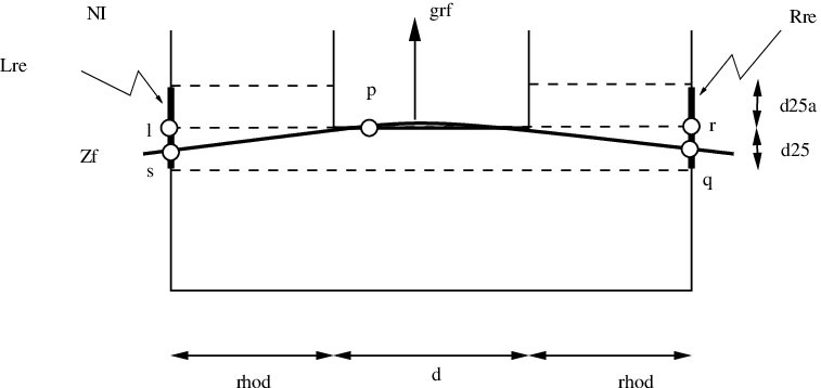
Proof.
1. There is a point on between the points of intersection with at which the gradient of is perpendicular to . See Figure 6. The small normal variation condition implies that does not intersect any of the two edges of parallel to , and that it intersects each of the edges of perpendicular to transversally in exactly one point. Let be the point of intersection with the edge containing . Then there is a point on at which the gradient of is perpendicular to the line segment . Since the angle between the gradients of at two points of does not differ by more than , we have . Therefore,
In other words, intersects . Similarly, intersects . The small normal variation condition implies that there are no other intersections with the edges of .
2. Let the points of intersection of and and be and , respectively. Then there is a point on at which is perpendicular to . Since the angle of and the vertical direction is at most
it follows from the small normal variation condition that the gradient of at any point of makes an angle of at most with the vertical direction. This rules out multiple intersections with the vertical edges of . It also implies that lies above the polyline , where is the intersection of the line through with slope and the line through with slope . Therefore, all points of lie at distance at most from the line through , so does not intersect the edges of parallel to . ∎
3.3 Towards an algorithm
After the first subdivision step, we have constructed a finite set of boxes, all of the same size, such that holds for each box . For each grid-box , the algorithm calls one of the following:
- •
Discard(), if it decides that does not contain a solution. It marks box as processed.
- •
ReportSolution(). It returns the certified pair , and marks all boxes contained in as processed.
In the latter case a solution is found inside , but, as will become clear later, it may not be contained in the smaller box . In view of none of the grid-boxes in contain a solution different from the one reported, so they are marked as being processed.
Decisions are based on evaluation of the signs of and at the vertices of the grid-boxes (or at certain dyadic points on edges of grid-boxes). An edge of a box is called bichromatic (monochromatic) for if the signs of the value of at its vertices are opposite (equal).
Algorithm, case 1: has a bichromatic edge for and a bichromatic edge for
Then and intersect , and, according to Lemma 3.2, part 1, both curves intersect the boundary of transversally in exactly two points. For each of the two points in the algorithm computes an isolating interval—called an -interval—on of length . The two -intervals are computed similarly. If the - and -intervals are not interleaving, there is no solution of (1) in box —even though there may be a solution in —and Discard() is called. This follows from Lemma 3.2, part 2. If the intervals are interleaving, then there is a point of intersection inside , so the algorithm calls ReportSolution().
Algorithm, case 2: contains no bichromatic edge for (), and at least one bichromatic edge for (, respectively)
We only consider the case in which all edges of are monochromatic for . Then the algorithm also evaluates the sign of at the vertices of the box . If has no disjoint bichromatic edges (as in the fourth and fifth configuration of Figure 7), the isocurve does not intersect , so the algorithm calls Discard().

To deal with the remaining case, in which has two disjoint bichromatic edges (as in the sixth configuration in Figure 7) we need to evaluate the sign of at certain dyadic points of these bichromatic edges, followed from Lemma 3.3. By evaluating the signs of at the (dyadic) endpoints of the interval and the algorithm decides whether they contain a point of intersection with . If at least one of these intervals is disjoint from , then Discard() is called. Otherwise, the algorithm computes isolating - and -intervals of length . As in case 1, the algorithm calls ReportSolution() if these intervals are interleaving, and Discard() otherwise.
Algorithm, case 3: all edges of are monochromatic for both and
Again, let be the (unique) edge of closest to the edge of which is
monochromatic for , at whose vertices the sign of is the opposite of the sign
of at the vertices of .
Edge of is defined similarly for .
Case 3.1: .
In this case or does not intersect . Indeed,
if intersects , it intersects in at least two points, so there is
a point at which is perpendicular to .
Condition guarantees that is nowhere parallel to
, so does not intersect , and, hence, does not intersect
. Therefore, Discard() is called.
Case 3.2: .
If does not intersect or , or
if does not intersect or , then, as in
case 2, the algorithm calls Discard().
Otherwise, or are isolating -intervals which are
disjoint from the isolating -intervals or .
If and are perpendicular, then these - and -intervals are
interleaving, and, hence, ReportSolution() is called. Otherwise, there is
no solution in , so Discard() is called.
Refinement: disjoint surrounding boxes
We would like distinct isolating boxes to have disjoint surrounding boxes . There is a simple way to ensure this: we just use the predicate to instead of in the above subdivision process. Then, if the interior of is non-empty, we can discard any one of or .
4 Isolating boxes for sinks, sources and saddles
In a first step, described in Section 3, we have constructed certified disjoint isolating boxes the singular points of in the domain of . Let be the closure of . Obviously, is a compact subset of .
In a second step towards the construction of the MS-complex, we refine the saddle-, sink- and sourceboxes. In Section 4.1 we show how to augment each saddlebox by computing four arbitrarily small disjoint intervals in its boundary, one for each intersection of a stable or unstable separatrix with the box boundary. Subsequently, in Section 4.2, we show how to construct for each source or sink of (minimum or maximum of ) a box on the boundary of which the gradient field is pointing outward or inward, respectively. These boxes are contained in the source- and sinkboxes constructed in the previous section, but are not necessarily axes-aligned.
4.1 Refining saddle boxes: Isolating separatrix intervals
To compute disjoint certified separatrix intervals we consider wedge shaped regions with apex at the saddle point, enclosing the unstable and stable manifolds of the saddle point. Even though the saddle point is not known exactly, we will show how to determine certified intervals for the intersection of these wedges and the boundary of a saddle box.
First we determine the eigenvalues and eigenvectors of the Hessian of at a point in the interior of the saddlebox —its center point, say—and consider these as good approximations to the eigenvalues and eigenvectors of the Hessian, i.e., the linear part of , at the saddle point. Let be the Hessian, i.e.,
| (3) |
and let be the Hessian evaluated at . The eigenvalues and of are given by
and the corresponding eigenvectors are
| (4) |
The singular point is a saddle, so we have . Since is a symmetric matrix, its eigenvectors are orthogonal. More precisely,
Here denotes counterclockwise rotation over an angle . Therefore,
| (5) |
The stable and unstable eigenvectors and are good approximations of the tangent vectors of the stable and unstable manifolds of the saddle point. These invariant manifolds are contained in wedge-shaped regions, which are defined as follows.
Definition 4.1.
Let the (orthogonal) vectors and be the stable and unstable eigenvectors of the Hessian of at the center of a saddle box , and let . The unstable wedge is the set of points in the surrounding box at which the (unsigned) angle between and is at most . See Figure 8. Similarly, the stable wedge is the set of points in the surrounding box at which the (unsigned) angle between and is at most .

The saddle point belongs to both the stable and the unstable wedge. Since and are orthogonal, and , this is the only common point of the stable and unstable wedge.
Conditions
We now introduce additional conditions, which guarantee that each of the wedge-boundaries consist
of two regular curves, cf lemma 4.2. In fact, these conditions
guarantee that and are really wedge-shaped.
Fix , and let be an arbitrarily small constant (to be specified
later).
At the point we have ,
, so can be taken small enough to guarantee
that the following condition is satisfied at all points of :
Condition I(). At every point of the box the following inequalities
hold:
At the point we also have , , and . Therefore, for any , the box can be taken small enough such that the following condition holds:
Condition II(). At every point of the box the following inequalities hold:
| (6) | ||||
| (7) | ||||
| (8) |
Since is symmetric, (8) also implies .
On the boundary of the gradient field makes a (signed) angle or with , or, in other words, is (anti)parallel to . Again, is the vector field obtained by rotating over an angle . So let be the curve along which the vector field is (anti)parallel to the unstable eigenvector . Then the boundary of the unstable wedge is the union of the two curves and . The curve is defined by the equation
| (9) |
Obviously, the saddle point lies on . The function is defined similarly.
Similarly, the boundary of the stable wedge is the union of curves , along which the vector field is (anti)parallel to . The curves are defined by the equation
The following technical result provides computable upper bounds for the angle variation of the normals of the boundary curves of the stable and unstable wedges.
Lemma 4.2.
Let (to be specified later), let , and let be such that Condition holds. Let and such that
| (10) | ||||
| (11) | ||||
| (12) |
If Condition also holds, then at any point of
| (13) |
and
| (14) |
In particular, the angle variation of any of the gradients and over is less than .
Proof.
We only show that the angle variation of over is less than . Since
the function satisfies where
so
Therefore,
| (15) |
Condition implies that , and are independent vectors, at all points of , so the gradient of is nonzero at every point of , so is a regular curve.
Expression (15) for implies that
Using the Cauchy-Schwarz inequality and the fact that we get
| (16) |
Since and , it follows from Condition that
Using Condition I again we get
In view of (16) we get, using :
| (17) |
Expression (15) for also implies that
Condition II and (12) imply
Since , this implies on .
The main result of this subsection states that, under suitable conditions, the intersection of the boundary of a saddle box and the stable and unstable wedges can be computed. Moreover, at all points of these intersections the gradient vector field is transversal to the boundary of the saddle box, and, even stronger, at these points there is a computable positive lower bound for the angle of the gradient vector field and the boundary of the saddle box.
Corollary 4.3.
If is a saddle box with concentric surrounding box satisfying Condition and Condition , then
- 1.
The saddle point is the only common point of the stable wedge and the unstable wedge .
- 2.
The gradient vector field is transversal at points on the boundary of these wedges, different from the saddle point: on the boundary of the unstable wedge it points inward, except at the saddle point, and on the boundary of the stable wedge it points outward, except at the saddle point.
- 3.
The unstable wedge contains the unstable separatrices of the saddle point, and the stable wedge contains the stable separatrices.
- 4.
The unstable wedge intersects the boundary of in two intervals, called the unstable intervals. Similarly, the stable wedge intersects the boundary of in two intervals, called the stable intervals. These four intervals are disjoint, and the unstable and stable intervals occur alternatingly on the boundary of . At each point of a stable or unstable interval the (unsigned) angle between and the boundary edge containing this point is at least . Moreover, there are computable isolating intervals for each stable and unstable interval.
Proof.
1. If , then
makes an angle with both
and . Therefore, , since these vectors
are orthogonal. Hence, is a singular point of inside
, which is the saddle point.
2. Recall from Lemma 4.2 that
is positive on . Let be the saddle
point of in . Since is parallel to on one
component of , and parallel to on the other
component, it follows that is pointing into the unstable wedge along both
components. See again Figure 8. Since is
obtained by rotating over , and over ,
also is pointing into the unstable wedge.
Similarly,
is negative along both components of , so
is also pointing into the unstable wedge along each of these
components.
A similar argument shows that is pointing outward
along each of the boundary components of the stable wedge ,
except at the saddle point.
3. The second part of the lemma implies that the unstable wedge is
forward invariant under the flow of the gradient vector field
. In particular, it contains the unstable separatrices of
the saddle point.
Similarly, the stable wedge is backward invariant, so it contains the
stable separatrices of the saddle point.

4. Suppose intersects an edge of the surrounding
box at a point , see Figure 9.
We first show that the angle of and is bounded
away from zero.
To see this, observe that there is a point at
which is perpendicular to .
Therefore, the angle between and the normal
of is at least , where
.
The angle between and lies in the
interval ,
cf Lemma 4.2, so the angle between and
is at least .
At any point of the angle between and is at most —by the definition of —so at any point of the angle between and is at least .
To find isolating intervals for the intersection of the stable and unstable wedges with the boundary of the surrounding box , we compute isolating intervals for the intersection of each of the four curves with this boudary. The normal to each of the curves makes an angle of at least with each of the curves . This follows from (13) and (14), and the fact that and are perpendicular. Since , so the angle between each of the curves and each of the curves is at least , which is bounded away from zero. Therefore, the method of Section 3 provides such isolating intervals. ∎
As will become clear in the certified construction of the MS-complex, we need to be able to provide certified separatrix intervals of arbitrarily small width, without refining the saddle box:
Lemma 4.4.
Let be a separatrix box satisfying the conditions of Corollary 4.3. Then the isolating separatrix intervals in the boundary of can be made arbitrarily small.
The proof of this result is rather technical. For a sketch we refer to B.
4.2 Refining boxes for maxima and minima
To construct the MS-complex, the algorithm needs to determine when an unstable (stable) separatrix will have a given maximum (minimum) of as its -limit (-limit). For each maximum (minimum) the algorithm determines a certified box such that the gradient vector field points inward (outward) on the boundary of the box. Unfortunately, we cannot always choose an axis-aligned box, as will become clear from the following example.
Let , then the origin is a sink of the gradient vector field
This vector field is horizontal along the line , which intersects the horizontal edges of every axis aligned box centered at the sink . In other words, the vector field is not transversal on the boundary of any such box.
However, there is a box aligned with (approximations) of a pair of
eigenvectors of the linear part of the gradient vector field at (or,
near) its singular point, for which the vector field is transversal
to the boundary.
To see this, we refine the sink-box to obtain three concentric
axis aligned boxes , such that
(i) the edge length of , , is three times the edge length of
, and
(ii) the sink is contained in the inner box .
See also Figure 10.

Moreover, let and be the (orthogonal) eigenvectors of the Hessian matrix at the center of the boxes. These eigenvectors, corresponding to the eigenvectors and , are computed as in Section 4.1, cf (4).
We require that
(iii) the gradients of the two functions and , defined by
have small angle variation over the outer box . This condition is made precise in Lemma 4.5 below. Note that
| (18) |
where is again the Hessian matrix of at . Since this matrix is non-singular, we can find a triple of boxes , satisfying conditions (i), (ii) and (iii), such that is nearly constant over the outer box (again, this is made precise in Lemma 4.5). In particular, is nearly parallel to , since . Now construct boxes and , which are the smallest boxes enclosing and , respectively, with edges parallel to or .
Lemma 4.5.
Suppose on the outer box the following conditions hold:
- 1.
, for ;
- 2.
.
Then the gradient vector field is transversal to the boundary of .
Proof.
The second condition limits the variation of the angle of and the basis vectors and over . Using this bound, we use the same arguments as in Section 3, applied to the pair of boxes , , to show that the curve does not intersect the edges of perpendicular to . Therefore, is nowhere zero on these edges, so is nowhere tangent to these edges. Therefore, is the desired sink box, on the boundary of which is pointing inward. In other words, if an unstable separatrix intersects the boundary of this box, the part of the separatrix beyond this point of intersection lies inside the sink-box. Certified source-boxes are constructed similarly. ∎
5 Isolating funnels around separatrices
If the forward orbits of the endpoints of an unstable separatrix interval have the same sink of as -limit, these forward orbits bound a region around the unstable separatrix leaving the saddle box via this unstable segment. This region is called a funnel for the separatrix (this terminology is borrowed from [16]).
In this section we provide the details of the construction of a certified funnel for each separatrix. First we show, in Section 5.1 how to construct two polylines per separatrix interval those are candidates for the funnel around the corresponding separatrix. Then, in Section 5.2, we introduce the notion of width of a funnel, and derive upper bounds for its growth. These upper bounds are the ingredients for a certified algorithm computing these funnels. The algorithm computes the Morse-Smale complex by providing disjoint certified funnels for each stable and unstable separatrix. The proof of correctness and termination is presented in Section 5.3.
5.1 Construction of fences around a separatrix
Let be the vector field obtained by rotating the vector field over an angle , i.e.,
We compute an isolating funnel for the forward orbit of through a point by enclosing it between (approximations of) the forward orbits of and through . See Figure 11.


Small angle variation
We first determine some bounds on the angle variation of the gradient vector field over . We subdivide the region into square boxes over which the angle variation of is at most , where is to be determined later. Let be the edge length of the boxes. If is a vector field on , then the angle variation over a regular curve is given by [2, Section 36.7]:
If , this angle variation is equal to
Let and be constants such that
| (19) |
Then the angle variation over a curve is less than
This inequality provides an upper bound for the maximal angle variation over a square box:
Lemma 5.1.
Let and satisfy (19). Then the total angle variation over a square box in with edge length does not exceed .
The grid boxes have edge length such that the angle variation of over any box in is less than .
Lemma 5.2.
Let , and let the grid boxes in have width satisfying
| (20) |
Then the following properties hold.
1. The angle variation of over any gridbox is less than
.
2. Let be a point on an edge of a gridbox,
and let be the point on the boundary of the gridbox into
which is pointing, such that the line segment
has direction .
The point is defined similarly. See Figure 12.
Then is pointing rightward along and
leftward along .
3. The function is strictly increasing on the line segments from to
and from to .

Proof.
The first claim follows from Lemma 5.1, using the fact that the diameter of a grid box is .
With regard to the second claim, the small angle variation condition implies that the orientation of does not change as ranges over . Since this orientation is positive for , it is positive for all . Similarly, the orientation of is negative for all . Therefore, the second claim also holds.
At a point of the line segment the directional derivative of in the direction of this line segment is , which is positive since the angle between and , is less than , and . This proves the third part. ∎
Fencing in the separatrices
For each isolating unstable separatrix interval on the boundary of a saddle box we construct two polylines and as follows. The initial points of these polylines are the endpoints of , and , where comes before in the counterclockwise orientation of the boundary of the saddle box. The polyline is uniquely defined by requiring that its vertices lie on grid edges, with the property that
- 1.
The line segment , , lies in a (closed) grid box of , and has direction .
- 2.
, the last vertex, lies on the boundary of .
The polyline is defined similarly, with the obvious changes: its initial vertex is , and each edge has direction equal to the value of the vector field at the initial point of this edge. The polylines are called fences of the (unique) unstable separatrix of intersecting .
It is not hard to see that that a grid box contains at most two consecutive edges of each of these polylines, but it is not obvious a priori that each box cannot contain more than two edges of each polyline in total. It follows from the next result that the intersection of a grid box with any of these polylines is connected, and, hence, that these polylines are finite.
The following results states that, when walking along the polylines and in the direction of increasing -values, each grid box is passed at most once.
Lemma 5.3.
Let be a box such that the angle variation of over the surrounding box is at most . Then the intersection of and ( and ) is either empty or a connected polyline (consisting of one or two segments).

Proof.
Let be a point at which leaves , i.e., the segment of ending at lies inside and the segment beginning at lies outside . Let be a point on the boundary of at which attains its maximum value .
Case 1: is a vertex of , incident to the edge of
containing .
See Figure 13, top row.
Let be the line through the edge of containing , let
be the angle between and , and let
be the angle between and the segment of
with initial point .
The angles and are both positive, since is a
vertex of .
The angle between and
is at most , since the angle variation of
over is less than .
Therefore, .
Let and , with and on the boundary of , be the line segments that make an angle of with . Since the angle variation of over is at most , the value of at any point of these line segments is at least . We shall prove that the connected component of containing intersects one of the line segments and .
First assume . Then the line segment lies in the grid box containing segment of . If lies on an edge of incident to , then intersects . So assume lies on the edge of contained in the boundary of (Figure 13, leftmost picture). Let be the point of intersection of the line through and the line through . This point lies on the same side of as and , since and . Furthermore, . Therefore, lies inside , in other words, intersects also in this case.
Now consider the case . Then lies on the side of parallel to the line through and . Furthermore, , so ‘leaves’ at a point on the side of perpendicular to the line through and . See Figure 13, rightmost picture. It follows that the part of between and intersects . In particular, .
Case 2: is not a vertex of , incident to the edge of containing . Then either is a vertex of , not incident to the edge of , containing , as in Figure 13, bottom-left picture, or lies on the relative interior of an edge of , as in Figure 13, bottom-right picture.
In this case is nearly vertical, as are the edges of . Similarly, the line segments and are nearly horizontal, so intersects . The details are similar to those of Case 1 of this proof. ∎
If the endpoints of the fences and lie on the same connected component of the boundary of , then these fences split into two connected regions. See Figure 14.

In this case, the region containing the separatrix interval in its boundary is called the funnel of (with angle ) denoted by . Its boundary consists of , the two fences and , and a curve on the boundary of connecting the endpoints of these fences. If the funnel is simply connected, it contains the part of the unstable separatrix through lying inside , which enters the funnel through and leaves it through . Note that is a curve either on the outer boundary of or on a sink box.
Similarly, each stable separatrix interval has two fences (for an angle ). If the endpoints of these fences lie on the same connected component of , the enclosed region is again called a funnel for the stable separatrix interval. Our goal is to construct disjoint, simply connected funnels for the stable and unstable separatrix intervals. If these funnels are disjoint, then they form, together with the sink boxes, source boxes and saddle boxes, a (fattened) Morse-Smale complex for .
It is intuitively clear that a funnel is simply connected if , the length of the separatrix interval , and the edge length of the grid boxes are sufficiently small. The next subsection presents computable upper bounds on these quantities, guaranteeing that the endpoints of two fences of a separatrix interval lie on the same boundary component. It is then easy to check whether the enclosed funnel is simply connected.
5.2 Controlling the width of the funnel
If the width of a funnel is sufficiently small, in a sense to be made more precise, it encloses a simply connected region in . The width of a funnel is, roughly speaking, the number of grid boxes between its bounding fences in the vertical direction, in regions where the fences are nearly horizontal, and in the horizontal direction, in regions where the fences are nearly vertical. To define the width of a funnel more precisely, we distinguish quasihorizontal and quasivertical parts of a funnel, and show that the width of a funnel does not increase substantially at transitions between these quasihorizontal and quasivertical parts.
Quasihorizontal and quasivertical parts of a funnel
A nonzero vector is called quasihorizontal if , and quasivertical if . Note that each nonzero vector is quasihorizontal, quasivertical, or both. Consider a subdivision of into boxes of equal width, where non-disjoint boxes share either an edge or a vertex. A horizontal -strip is the union of a sequence of boxes where successive boxes share a vertical edge, such that the horizontal edge of the rectangle thus obtained has length at most . A vertical -strip is defined similarly. An -box is a square box with edge length at most which is the union of a number of boxes. Two polygonal curves and form an -funnel if there is a set of horizontal -strips, a set of vertical -strips, and a set of -boxes such that the following holds:
- 1.
The vertices of and lie on the edges of the grid-boxes; intersects a grid box in at most one vertex or in at most one edge; the same holds for ;
- 2.
Both and lie in the union of the rectangles in , and ;
- 3.
An edge of contained in a horizontal -strip is quasi-vertical, and an edge contained in a vertical -strip is quasihorizontal. Moreover, neither nor intersect the vertical sides of a horizontal -strip, or the horizontal sides of a vertical -strip. Each -strip and each -box is intersected by both polylines.
- 4.
Either or intersects an -box in exactly one of its edges, which is contained in a grid box at the corner of the -box. This single edge is either quasivertical or quasihorizontal (but not both). If this edge is quasihorizontal (quasivertical), all edges of the other polyline inside the -box are quasihorizontal (quasivertical) as well – and possibly also quasivertical (quasihorizontal). The other polygonal curve intersects the same edges of the -box, each in exactly one point, and is disjoint from the other edges of the -box.
See also Figure 15.

We determine later, but for now we assume that
| (21) |
We start with a simple observation.
Lemma 5.4.
Let be a polyline with quasihorizontal edges and with vertices on the edges of a grid with edge length satisfying (20). If lies in a vertical strip of width , where each of the vertical lines bounding the strip contains one of its endpoints, then intersects at most three grid boxes contained in this vertical strip.
A similar property holds for a polyline with quasivertical edges intersecting a horizontal strip.
Proof.
We only prove the first part, in which lies in a vertical strip and has quasihorizontal edges. The slope of the line segment connecting the endpoints of does not exceed the maximum slope of any of the edges of , so this slope is at most . Hence the projection of this line segment on any of the vertical lines bounding the strip has length at most , so it intersects at most three boxes. ∎
The next result shows that the width of a funnel does not grow substantially at a transition between a quasihorizontal and a quasivertical part. We take such that the angle variation of over a box with edge length is at most . Again, by Lemma 5.1, this is guaranteed by taking
| (22) |
Lemma 5.5.
Let be an -box intersected by both and , with an edge which contains the initial vertex of both and . Assume that at least one of the polylines has an edge which is either quasihorizontal or quasivertical, but not both. Then both polylines intersect the boundary of in exactly two points, and there is an edge of , adjacent to , containing the terminal vertices of both and . See Figure 15.
Proof.
Assume that has an edge which is quasivertical but not quasihorizontal. We first show that all edges of are quasivertical (and possibly quasihorizontal). The angle between and the horizontal direction is at least , which is greater than . Since the slope of is the slope of the vector field at the initial vertex of , and the angle variation of over is at most , the slope of at any point of is at least . Since the slope of an edge of is the slope of at the initial vertex of this edge, we conclude that all edges of are quasivertical.
All edges of are also quasivertical (and possibly quasihorizontal). To see this, observe that the slope of an edge of is the slope of at the initial vertex of this edge, and, hence, the slope of at this initial vertex, minus . In other words, the slope of any edge of is at least . Since , this slope is at least . Therefore, all edges of are quasivertical.
The polylines and do not intersect the
edge of opposite , since then at least one of the edges of these polylines
would have a slope less than .
Let be the edge containing the endpoint of .
Then is adjacent to .
Given the bounds on the slope variation of the edges of the polylines, it is
easy to see that
(i) the endpoint of is the only point of this polyline on ;
(ii) the endpoint also lies on , and this is the only
point of this polyline on ;
(iii) none of the polylines intersects the edge opposite .
This concludes the proof of Lemma 5.5.
∎
Growth of the width of quasihorizontal and quasivertical funnel parts
The width of the funnel may grow exponentially in the number of grid boxes it is traversing. The next result gives an upper bound for the growth of this width. Even though the bounds are conservative, they provide the tools for the construction of certified funnels for all separatrices.
A gridbox is called quasihorizontal (quasivertical) if it contains a point at which is quasihorizontal (quasivertical). Again, a gridbox may be both quasihorizontal and quasivertical.
An integral curve of in a quasihorizontal gridbox is the graph of a function , where is a solution of the differential equation
| (23) | ||||
where . Here ranges over the full interval if . Otherwise, the range of is restricted to a suitable maximal subinterval , such that and are points on the boundary of the gridbox. Similarly, a trajectory of in a quasihorizontal gridbox is the graph of a function , where is a solution of the differential equation
| (24) |
with
Similarly, a trajectory of is the graph of a function , where is a solution of the differential equation
with
Here ranges over the full interval if , or a suitable maximal subinterval otherwise.
The union of all quasihorizontal gridboxes in is denoted by , and the union of all quasivertical gridboxes by .
Even though the width of a funnel may grow exponentially in the number of grid boxes it traverses, this growth is controlled. To this end, we introduce several computable constants that only depend on the function and (the size of) its domain . Let , , , , and be positive constants such that
Note that
Let be a dyadic number such that
| (25) |
Take such that . Finally, let be a constant such that
| (26) |
Taking , we have, for :
| (27) |
Similarly, there are (computable) constants and such that
| (28) |
for . Finally, let the constants , and be defined by
| (29) | ||||
| (30) | ||||
| (31) |
The next result provides an upper bound for the growth of the funnel width along a quasihorizontal part of its bounding polylines. We assume that the funnel runs from left to right, so its initial points are on the line with smallest -coordinate. If the funnel runs from right to left, a similar result is obtained.
Lemma 5.6.
Let be the piecewise linear functions the graphs of which are quasihorizontal parts of the polylines and for a grid with edge length , respectively. Let be an upper bound for the distance of the initial points of these polylines, i.e.,
Then the width of the fence, bounded by and , is bounded:
Proof.
Let be the exact solution of the rotated system with initial condition . In particular, . Then (27) implies
Therefore, according to the Fundamental Inequality [16, Theorem 4.4.1]—See also A—we have
| (32) |
The interval is subdivided into a finite number of subintervals of length at most , where the endpoints correspond to the -coordinates of the breakpoints of the fences and . Let be the Euler approximation to the ordinary differential equation (24). Its graph is (a quasihorizontal) part of the fence . Theorem 4.5.2 in [16]—See also A—gives the following explicit bound for the error in Euler’s method:
| (33) |
We get a similar inequality for the Euler approximation of . Combining (32) and (33), and using (29) and (30), yields
∎
A similar result holds for quasivertical trajectories. Next we need to control the increase of the funnel width upon transition from a quasihorizontal to a quasivertical part its bounding polylines (or from a quasivertical to a quasihorizontal part).
Transitions: bounded increase of funnel width
Transition from a quasihorizontal to a quasivertical, or from a quasivertical to a quasihorizontal part of the funnel takes place at an -box. If the width of the funnel at the ‘entry’ of the box is less than the width of a grid box, then the width may increase, but it will not be greater than at the exit. This is made more precise by the following result.
Lemma 5.7.
Let be a -box as in Lemma 5.5, where, moreover, the initial points and of and , respectively, are on the boundary of the gridboxes containing the vertices of edge of . If the distance between and is at least , then the distance between the terminal points and of and , respectively, is less than the distance of and . If the distance between and is less than , then the distance of and is at most .
Proof.
Assume that the first edge of is quasivertical, but not quasihorizontal. Edge of is then vertical. Assume that this polyline consists of a single edge, namely the line segment .

Let be the angle between and edge , then . Let be the angle between the line segment and edge , then is inbetween the smallest and largest slope of any edge of . Since the angle variation of over is less than , the angle is greater than . Let be the distance of to the nearest vertex of , then . If , the distance between and satisfies
since . Here we used to get
Since , a short computation shows that .
If , then lies in the same gridbox as , or in a gridbox adjacent to it. Then it is easy to see that lies in the same grid box as , and also lies in this box, or in a box adjacent to it. Therefore, in this case.
If consists of a single edge, then the argument is similar. ∎
Lemmas 5.6 and 5.7 provide the following result on the upper bound on the funnel width of a separatrix with transitions between quasihorizontal and quasivertical parts.
Corollary 5.8.
Let be the (computable) edge length of a bounding square of the domain of the function ), and let be the total number of quasihorizontal and quasivertical parts of the polylines bounding a separatrix funnel. Let and let . Then the width of the funnel does not exceed
provided where , with and given by (29) and (30), respectively.
In particular, this width is at most if
| (34) |
Proof.
Let , then . There are transitions from quasihorizontal to quasivertical parts of the funnel, each occurring at an -box. Let be the width of the initial separatrix interval, and let be the width of the funnel at the entry of the corresponding boxes, in other words, is the width at the end of the -th part of the funnel. Using induction, we will prove that, for :
| (35) |
So assume (35) holds for . If , the initial width of the -th part of the funnel does not exceed , cf Lemma 5.7. Assume that the -th part of the funnel is quasihorizontal, then Lemma 5.6 implies that the width of this part at a point with horizontal coordinate is at most
so in particular, since and :
Therefore, (35) holds for . If , then the initial width of the -th part of the funnel is at most , cf Lemma 5.7. Therefore, Lemma 5.6 implies that the width of this part at a point with horizontal coordinate is at most
so in particular
Therefore, for , we have
which proves the corollary. ∎
Remark 5.9.
The computable constants and depend only on and .
In the next section, we assemble the bits and pieces into a certified algorithm for the construction of the MS-complex, and show how the upper bounds on the funnel width are used to prove that this algorithm terminates.
5.3 Construction of the MS-complex
The Algorithm
The construction of the MS-complex of is a rather straightforward application of the preceding results. It uses a parameter , the (a priori unknown) number of transitions (at -boxes) between quasihorizontal and quasivertical parts of a funnel. Let be the edge length of a bounding square of the domain of . Then the algorithm performs the following steps.
-
Step 1. Construct certified isolating boxes for the singularities of (cf Section 3).
-
Step 2. Let be the closure of . Compute the constants , , , and , which depend only on and . Set to the minimum of the width of the source-, sink- and saddleboxes.
-
Step 3. Let and be such that , , and (cf Corollary 5.8). Subdivide until all gridboxes have maximum width . For each saddle box, compute four separatrix intervals on its boundary, of width at most .
-
Step 4. For each stable and unstable separatrix interval do the following. Start the computation of a funnel for a separatrix by setting to a small number (say 4). Compute the fences and , keeping track of the width of the enclosed funnel under construction and of the number of transitions between quasihorizontal and quasivertical parts of this funnel.
If the width of the funnel exceeds or the number of transitions exceeds , then abort the computation of the current funnel, discard all funnels constructed so far, set to twice its current value and goto Step 3.
If the funnel intersects an already constructed funnel, or a source- or sinkbox on which it does not terminate (i.e., if only one of its fences intersects this box), then set to half its current value, discard all funnels constructed so far, and goto Step 3.
If the funnel intersects a saddlebox , then decrease the size of by a factor of two via subdivision, discard all funnels constructed so far, set to half its current value, and goto Step 2. (Note that gets larger, so the constants in Step 2 have to be recomputed.)
Otherwise, the fences end on the same component of the boundary of . The enclosed funnel is simply connected, and does not intersect any of the funnels constructed so far. Add the funnel to the output, and reset to (and repeat until all separatrices have been processed).
5.4 Termination
Since the gradient field is a Morse-Smale system, its separatrices are disjoint. Their intersections with are compact, and have positive distance (although this distance is not known a priori). In the main loop of the algorithm, the maximal funnel width is bisected if funnels intersect, and saddleboxes intersected by the funnel are subdivided, so after a finite number of iterations of the main loop its value is less than half the minimum distance between any pair of distinct separatrices, and funnels stay clear from saddleboxes (apart from the one containing the - or -limit of the enclosed separatrix).
Separatrices that intersect do so transversally, cf Remark 2.1. Therefore, after a finite number of subdivision steps, both fences around such separatrices will intersect transversally. Hence, eventually all funnels become disjoint, at which point the algorithm terminates after returning a topologically correct MS-complex for .
6 Implementation and experimental results
The algorithm has been implemented using the Boost library [1] for IA. All experiments have been performed on a 3GHz Intel Pentium 4 machine under Linux with 1 GB RAM using the g++ compiler, version 3.3.5. Figures 11(a)-1(b) and 1717(a)-17(b) depict the output of our algorithm, for several Morse-Smale functions. In our implementation the parameter , used in the construction of separatrix-funnels, is , which is larger than the theoretical bound given by Corollary 5.8. The algorithm halves this angle several times, depending on the input, until the funnels are simply connected, mutually disjoint, and connect a saddle-box to a source-box (for stable separatrices) or sink-box (for unstable separatrices), in which case a topologically correct MS-complex has been computed.


Each of the funnels with deep black boundaries contains an unstable separatrix, whereas a funnel with light black boundaries contains a stable separatrix. The CPU-time for computing a MS-system increases with the number of critical points and the complexity of the vector field, as indicated in the captions of the figures.
7 Conclusion
The outcome of our research is two-fold. Firstly, we compute the topologically correct MS-complex of a Morse-Smale system. The correct saddle-sink or saddle-source connectivity can also be represented as a graph, which is of special interest from different application point of view. On the other hand, depending on a user-specified width of funnel one can compute a geometrically close approximation of the MS-complex. We give the proof of convergence of our algorithms. Although the complexity of the given algorithm depends on the input function and the complexity of the interval arithmetic library used in the algorithm. As we discussed some of the separatrices inside a bounding box may have discontinuous components. The algorithm we propose here is able to compute only the part of the separatrices which are connected to the corresponding saddle. Therefore one open question is how to compute all the components of separatrices inside a bounding box.
References
- [1] Boost interval arithmetic library. http://www.boost.org.
- [2] V.I. Arnol’d. Ordinary Differential Equations. Universitext. Springer-Verlag, New York, Heidelberg, Berlin, 2006.
- [3] C.L. Bajaj and D.R. Schikore. Topology preserving data simplification with error bounds. Comput. Graph., 22(1):3–12, 1998.
- [4] T. F. Banchoff. Critical points and curvature for embedded polyhedral surfaces. Amer. Math. Month., 77:475–485, 1970.
- [5] S. Biasotti, L. De Floriani, B. Falcidieno, P. Frosini, D. Giorgi, C. Landi, L. Papaleo, and M. Spagnuolo. Describing shapes by geometrical-topological properties of real functions. ACM Computing Surveys, 40(4):12.1–12:87, 2008.
- [6] F. Cazals, F. Chazal, and T. Lewiner. Molecular shape analysis based upon the Morse-Smale complex and the Connolly function. In In SCG 2003: Proceedings of the 19th Annual Symposium on Computational Geometry, pages 351–360, ACM Press, New York, NY, 351-360, 2003.
- [7] A. Chattopadhyay, G. Vegter, and C.K. Yap. Certified Computation of Planar Morse-Smale Complexes. In Proceedings 27th ACM Symposium on Computational Geometry, pages 259–268, Chapel Hill, 2012.
- [8] S.-N. Chow and J.K. Hale. Methods of Bifurcation Theory, volume 251 of Grundlehren der mathematischen Wissenschaften. Springer-Verlag, New York, Heidelberg, Berlin, 1982.
- [9] E.A. Coddington and N. Levinson. Theory of Ordinary Differential Equations. McGraw-Hill Book Company, 1955.
- [10] H. Edelsbrunner, J. Harer, V. Natarajan, and V. Pascucci. Morse-Smale complexes for piecewise linear 3-manifolds. In Proc. 19th Ann. Sympos. Comput. Geom., pages 361–370, 2003.
- [11] H. Edelsbrunner, J. Harer, and A. Zomorodian. Hierarchical Morse-Smale complexes for piecewise linear 2-manifolds. Discrete Comput. Geom, 30:87–107, 2003.
- [12] R. Forman. Morse theory for cell complexes. Adv. Math., 134:90–145, 1998.
- [13] A. Gyulassy, P. Bremer, B. Hamann, and V. Pascucci. A practical approach to Morse-Smale complex computation. IEEE Transactions on Visualization and Computer, 14:1619–1626., 2008.
- [14] J. L. Helman and L. Hesselink. Visualizing vector field topology in fluid flows. IEEE Computer Graphics and Applications, 11(3):36–46, 1991.
- [15] M. W. Hirsch and S. Smale. Differential Equations, Dynamical Systems, and Linear Algebra. Academic Press, 1974.
- [16] J.H. Hubbard and B.H. West. Differential Equations. A Dynamical Systems Approach. Part I, volume 5 of Texts in Applied Mathematics. Springer Verlag, New York, Heidelberg, Berlin, 1991.
- [17] C. Li, S. Pion, and C. Yap. Recent progress in Exact Geometric Computation. J. of Logic and Algebraic Programming, 64(1):85–111, 2004. Special issue on “Practical Development of Exact Real Number Computation”.
- [18] Long Lin and Chee Yap. Adaptive isotopic approximation of nonsingular curves: the parameterizability and nonlocal isotopy approach. Discrete and Computational Geometry, 45(4):760–795, 2011.
- [19] F. Meyer. Topographic distance and watershed lines. Signal Process., 38:113–125, 1994.
- [20] J. Milnor. Morse Theory. Princeton University Press, 1968.
- [21] R.E. Moore. Interval Analysis. Prentice-Hall., 1996.
- [22] J. Palis and W. de Melo. Geometric Theory of Dynamical Systems: An Introduction. Springer-Verlag, 1982.
- [23] S. Plantinga and G. Vegter. Isotopic meshing of implicit surfaces. The Visual Computer, 23:45–58, 2007.
- [24] J. M. Snyder. Generative modeling for computer graphics and CAD: symbolic shape design using interval analysis. Academic Press Professional, Inc., San Diego, CA, USA, 1992.
- [25] J. M. Snyder. Interval analysis for computer graphics. SIGGRAPH Computer Graphics, 26(2):121–130, 1992.
- [26] J.M. Snyder. Generative Modeling for Cimputer Graphics and CAD. Symbolic Shape Design Using Interval Analysis. Academic Press Professional, Inc., San Diego, CA, USA, 1992.
- [27] J.M. Snyder. Interval analysis for computer graphics. SIGGRAPH Comput. Graph., 26(2):121–130, 1992.
- [28] S. Takahashi, T. Ikeda, Y. Shinagawa, and I. Fujishiro. Algorithms for extracting correct critical points and constructing topological graphs from discrete geographic elevation data. Comput. Graph. For., 14(3):181–192, 1995.
- [29] C.K. Yap. In praise of numerical computation. In S. Albers, H. Alt, and S. Näher, editors, Efficient Algorithms, volume 5760 of Lecture Notes in Computer Science, pages 308–407. Springer-Verlag, 2009. Essays Dedicated to Kurt Mehlhorn on the Occasion of His 60th Birthday.
- [30] E. Zhang, K. Mischaikow, and G. Turk. Vector field design on surfaces. ACM Transactions on Graphics, 25(4):1294–1326, 2006.
Appendix A Mathematical results used in the text
Error in Euler’s method.
Error bounds for approximate solutions of ordinary differential equation play a crucial role in the construction of certified funnels for separatrices. We quote the relevant parts of the book [16].
Fundamental Inequality [16, Theorem 4.4.1].
Consider the differential equation
on a box , and let be a constant such that
If and are two approximate piecewise differentiable solutions satisfying
for all at which and are differentiable, and if, for some
then, for all
where .
The well-known Euler method for constructing approximate solutions to ordinary differential equations is also useful for the construction of certified strips. It proceeds as follows. For a given initial position , define the sequence of points by
as long as . Then the Euler approximate solution through with step is the piecewise linear function the graph of which joins the points , so
The following result states that the Euler approximate solution converges to the actual solution as the step tends to zero, and gives a bound for the error.
Error in Euler’s method [16, Theorem 4.5.2].
Consider the differential equation
on a box , where is a -function on . Let the constants , and satisfy
The deviation of the Euler approximate solution with step from a solution of the differential equation with satisfies
for all .
The preceding result also holds if, as in the current chapter, is not the exact step, but an upper bound for a possibly varying step.
Appendix B Narrowing separatrix intervals
We first sketch the algorithm for narrowing the separatrix intervals. To this end we subdivide the box , and hence the box , yielding a nested sequence of boxes , with surrounding boxes , such that
- 1.
- 2.
the saddle point is contained in box , for all .
See Figure 18.

Let be the -coordinate of the saddle point , and let be the -coordinate of the rightmost vertical boundary edge of . Let be the width of , and let be the -coordinate of its center. Then , and . Since then , since
Since , we get
| (36) |
Consider the forward integral curves of the vector field through the points of intersection of the line and the boundary curves . See Figure 19. These curves intersect the rightmost edge of in two points bounding an interval on this edge. Arbitrarily good approximations of these integral curves are obtained as follows. Let be (an upper bound on) the maximum angle variation of over any of the boxes of the -th subdivision of . Since is , the angle variation is a Lipschitz function, so . In particular, the rotated vector fields converge to . We construct an upper fence with angle for the upper integral curve, and a lower fence with angle for the lower integral curve. See also Section 5.1 for the construction of a fence. These fences are disjoint, since the angle variation of over a grid box is less than .
Since , cf (36), the points converge to the saddle point. Therefore, the intervals , contained in the intersection of the unstable wedge and the rightmost vertical edge of , converge to the intersection of the unstable separatrix and the rightmost vertical edge of .

A proof of Lemma 4.4 can be given along the lines of [9, page 330ff] or [8, Chapter 3.6]. Rather than giving a complete proof we give an example illustrating the main ideas. Consider the function , with . The gradient vector field is given by . Obviously, the origin is a saddle point, with positive eigenvalue and negative eigenvalue , and eigenvectors and , respectively. The unstable cone of this saddle point is bounded by the curves , defined implicitly by , where
Therefore, the equation of is , with . Let the right vertical edge of be on the line , , and consider a point , with , on the boundary curve of the unstable cone. The integral curve of through satisfies the differential equation
with initial condition , where . Therefore,
The integral curve through intersects the rightmost edge of in the point , where
Similarly, the integral curve through intersects the rightmost edge of in the point . Now let range over the sequence . Then the interval has endpoints , so its width is . In view of (36), with , we have
In other words, with and ,
Hence,
Since , after two subdivision steps the size of the separatrix interval reduces by more than a factor two. Hence interval arithmetic provides an arbitrarily good approximation of the intersection of the unstable separatrix and the boundary of the saddle box. A similar observation holds for the intersection of the other separatrices and the boundary of their saddle box.