Vectorlike -boson coupling at TeV and third family fermion masses
Abstract
In the third fermion family and gauge symmetry of the Standard Model (SM), we study the quark-quark, lepton-lepton and quark-lepton four-fermion operators in an effective theory at high energies. These operators have nontrivial contributions to the Schwinger-Dyson equations for fermion self-energy functions and the -boson coupling vertex. As a result, the top-quark mass is generated via the spontaneous symmetry breaking of -condensate and the -boson coupling becomes approximately vectorlike at TeV scale. The bottom-quark, tau-lepton and tau-neutrino masses are generated via the explicit symmetry breaking of -contributions and quark-lepton interactions. Their masses and Yukawa couplings are functions of the top-quark mass and Yukawa coupling. We qualitatively show the hierarchy of fermion masses and Yukawa couplings of the third fermion family. We also discuss the possible collider signatures due to the vectorlike (parity-restoration) feature of -boson coupling at high energies.
pacs
12.60.-i,12.60.Rc,11.30.Qc,11.30.Rd,12.15.FfI Introduction
The parity-violating (chiral) gauge symmetries and spontaneous/explicit breaking of these symmetries for the hierarchy of fermion masses and mixing angles have been at the center of a conceptual elaboration that has played a major role in donating to mankind the beauty of the SM for fundamental particle physics. On the one hand the composite Higgs-boson model or the Nambu-Jona-Lasinio (NJL) [1] with four-fermion operators, and on the other the phenomenological model [2] of the elementary Higgs boson, they are effectively equivalent for the SM at low energies and provide an elegant and simple description for the electroweak symmetry breaking and intermediate gauge boson masses. The experimental results of Higgs-boson mass 126 GeV [3] and top-quark mass 173 GeV [4] begin to shed light on this most elusive and fascinating arena of fundamental particle physics.
In order to accommodate high-dimensional operators of fermion fields in the SM framework of a well-defined quantum field theory at the high-energy scale , it is essential and necessary to study: (i) what physics beyond the SM at the scale explains the origin of these operators; (ii) which dynamics of these operators undergo in terms of their dimensional couplings (e.g., ) and energy scale ; (iii) associating to these dynamics, where infrared (IR) and ultraviolet (UV) stable fixed points of these couplings locate and what characteristic energy scale is; (iv) in the IR domain and UV domain (scaling regions) of these stable IR and UV fixed points, which operators become physically relevant (effectively dimension-4) and renormalizable following renormalization group (RG) equations (scaling laws), and other irrelevant operators are suppressed by the cutoff at least .
The strong technicolor dynamics of extended gauge theories at the TeV scale was invoked [5, 6] to have a natural scheme incorporating the relevant four-fermion operator
| (1) |
of the -condensate model of Bardeen, Hill and Lindner (BHL) [7] and notations will be given later in Eq. (10). This relevant four-fermion operator (1) undergoes the dynamics of spontaneous symmetry breaking (SSB) in the IR domain (small ) of infrared fixed point (critical value) associated with the SSB and characteristic energy scale (vev) GeV. The analysis of this composite Higgs boson model was made [7] to show the low-energy effective Lagrangian, RG equations, the composite Goldstone modes (pseudoscalars ) for the longitudinal modes of massive and gauge bosons, and the composite scalar () for the Higgs boson in the SM. On the other hand, these relevant operators can be constructed on the basis of phenomenology of the SM at low-energies. In 1989, several authors [7, 8, 9] suggested that the symmetry breakdown of the SM could be a dynamical mechanism of the NJL type that intimately involves the top quark at the high-energy scale . Since then, many models based on this idea have been studied [10]. The low-energy SM physics was supposed to be achieved by the RG equations in the IR domain of the IR-stable fixed point with GeV [6, 9, 7].
Nowadays, the top-quark and Higgs boson masses are known and they completely determine the boundary conditions for the RG equations of the composite Higgs boson model [7]. Using the experimental values of top-quark and Higgs boson masses, we obtained [11, 12] the unique solutions to these RG equations provided the appropriate nonvanishing form factor of the composite Higgs boson in TeV scales where the effective quartic coupling of composite Higgs bosons vanishes.
The form factor of composite Higgs boson is finite and does not vanish in the SSB phase (composite Higgs phase for small ), indicating that the tightly bound composite Higges particle behaves as if an elementary particle. On the other hand, due to large four-fermion coupling , massive composite fermions are formed by combining a composite Higgs boson with an elementary fermion in the symmetric phase where the SM gauge symmetries are exactly preserved [13]. This indicates that a second-order phase transition from the SSB phase to the SM gauge symmetric phase takes place at the critical point . In addition the effective quartic coupling of composite Higgs bosons vanishing at TeV scales indicates the characteristic energy scale of such phase transition. The energy scale is much lower than the cutoff scale () so that the fine-tuning (hierarchy) problem of fermion masses or the pseudoscalar decay constant can be avoided [11].
In this article, after a short review that recalls and explains the quantum-gravity origin of four-fermion operators at the cutoff , the SSB and -condensate model, we show that due to four-fermion operators (i) there are the SM gauge symmetric vertexes of quark-lepton interactions; (ii) the one-particle-irreducible (1PI) vertex function of -boson coupling becomes approximately vectorlike at TeV scale. Both interacting vertexes contribute the explicit symmetry breaking (ESB) terms to Schwinger-Dyson (SD) equations for fermion self-energy functions. As a result, once the top-quark mass is generated via the SSB, other fermion masses are generated by the ESB via quark-lepton interactions and -boson vectorlike coupling. In the third fermion family, we qualitatively show the hierarchy of fermion masses and effective Yukawa couplings in terms of the top-quark mass and Yukawa coupling. In the concluding section, a summary of basic points of the scenario and its extension to three fermion families is given. In addition, we present some discussions on the possible experimental relevance of running Yukawa couplings obtained and parity-conservation feature of the -boson coupling at TeV scale 11 1 More discussions on the experimental aspects of this scenario can be found in the Refs. S.-S. Xue, arXiv1601.06845 and arXiv1506.05994v2. The latter contains the part of this article..
II Four-fermion operators from quantum gravity
A well-defined quantum field theory for the SM Lagrangian requires a natural regularization (cutoff ) fully preserving the SM chiral-gauge symmetry. The quantum gravity naturally provides a such regularization of discrete space-time with the minimal length [16], where the Planck length cm and scale GeV. However, the no-go theorem [17] tells us that there is not any consistent way to regularize the SM bilinear fermion Lagrangian to exactly preserve the SM chiral-gauge symmetries, which must be explicitly broken at the scale of fundamental space-time cutoff . This implies that the natural quantum-gravity regularization for the SM should lead us to consider at least dimension-6 four-fermion operators originated from quantum-gravity effects at short distances 22 2 In the regularized and quantized EC theory [16] with a basic space-time cutoff, in addition to dimension-6 four-fermion operators, there are high-dimensional fermion operators (), e.g., , which are suppressed at least by . .
On the other hand, it is known that four-fermion operators of the classical and torsion-free Einstein-Cartan (EC) theory are naturally obtained by integrating over “static” torsion fields at the Planck length,
| (2) |
where the gravitational Lagrangian , tetrad field , spin-connection field , the covariant derivative and the axial current of massless fermion fields. The four-fermion coupling relates to the gravitation-fermion gauge coupling and fundamental space-time cutoff .
Within the SM fermion content, we consider massless left- and right-handed Weyl fermions and carrying quantum numbers of the SM symmetries, as well as three right-handed Weyl sterile neutrinos and their left-handed conjugated fields , where “” is the fermion-family index. Analogously to the EC theory (2), we obtain a torsion-free, diffeomorphism and local gauge-invariant Lagrangian
| (3) | |||||
where we omit the gauge interactions in and axial currents read
| (4) |
The four-fermion coupling is unique for all four-fermion operators and high-dimensional fermion operators () are neglected. If torsion fields that couple to fermion fields are not exactly static, propagating a short distance , characterized by their large masses , this implies the four-fermion coupling . We will in the future address the issue of how the space-time cutoff due to quantum gravity relates to the cutoff scale possibly by intermediate torsion fields or the Wilson-Kadanoff renormalization group approach. In this article, we adopt the effective four-fermion operators (3) in the context of a well-defined quantum field theory at the high-energy scale .
By using the Fierz theorem [18], the dimension-6 four-fermion operators in Eq. (3) can be written as
| (5) | |||||
| (6) |
which preserve the SM gauge symmetries. Equations (5) and (6) represent repulsive and attractive operators respectively. In Ref. [19], we pointed out that the repulsive four-fermion operators (5) are suppressed by the cutoff , and cannot become relevant and renormalizable operators of effective dimension-4 in the IR domain where the SSB dynamics occurs.
Thus the torsion-free EC theory with the relevant four-fermion operators read,
| (7) | |||||
where the two-component Weyl fermions and respectively are the gauged doublets and singlets of the SM. For the sake of compact notations, is also used to represent , which has no SM quantum numbers. All fermions are massless, they are four-component Dirac fermions , two-component right-handed Weyl neutrinos and four-component sterile Majorana neutrinos whose kinetic terms read
| (8) |
In Eq. (7), and () are fermion-family indexes summed over respectively for three lepton families (charge ) and three quark families (). Equation (7) preserves not only the SM gauge symmetries and global fermion-family symmetries, but also the global symmetries for fermion-number conservations.
III The third fermion family
In this section, we discuss how the quark and lepton Dirac mass matrices are generated by the SSB via four-fermion operators. In Eq. (7), the four-fermion operators of the quark sector are
| (9) |
Due to the unique four-fermion coupling and the global fermion-family symmetry of Eq. (9), we perform chiral transformations and so that , the four-fermion operator (9) is only for each quark family and all quark fields are Dirac mass eigenstates. The four-fermion operators (9) read,
| (10) |
where and are the color and flavor indexes of the top and bottom quarks, the left-handed quark doublet and the right-handed singlet . The first and second terms in Eq. (10) are respectively the four-fermion operators of top-quark channel [7] and bottom-quark channel, whereas “terms” stands for the first and second quark families that can be obtained by substituting and .
In Eq. (7), the four-fermion operators relating to the lepton Dirac mass matrix are
| (11) |
where Dirac lepton fields and are the SM doublets and singlets respectively, and are three sterile neutrinos. Analogously to the quark sector (9), we perform chiral transformations and so that , the four-fermion operators (11) are only for each lepton family and all lepton fields are Dirac mass eigenstates. Namely, the four-fermion operators (11) become
| (12) |
where three right-handed sterile neutrinos (), the left-handed lepton doublets and the right-handed singlets .
In the IR domain of the SM, the four-fermion coupling and the SSB leads to the fermion-condensation , two diagonal mass matrices of quark sectors and satisfying mass-gap equations. It was demonstrated [20] that as an energetically favorable solution of the SSB ground state of the SM, only top-quark is massive (), otherwise there would be more Goldstone modes in addition to those becoming the longitudinal modes of massive gauge bosons. In other words, among four-fermion operators (10) and (12), the -condensate model (1) is the unique channel undergoing the SSB of SM gauge symmetries, for the reason that this is energetically favorable, i.e., the ground-state energy is minimal when the maximal number of Goldstone modes are three and equal to the number of the longitudinal modes of massive gauge bosons in the SM. Moreover, the four-fermion operators (11) of the lepton sector do not undergo the SSB leading to the lepton-condensation , i.e., two diagonal mass matrices of the lepton sector ( and ). The reason is that the effective four-lepton coupling is -times smaller than the four-quark coupling , where the color number . In the IR domain of the IR-stable fixed point (the critical value), the effective four-quark coupling is above the critical value and the SSB occurs, whereas the effective four-lepton coupling is below the critical value and the SSB does not occur.
As a result, only the top quark acquires its mass via the SSB and four-fermion operator (1) of the top-quark channel becomes the relevant operator following the RG equations in the IR domain [7]. While all other quarks and leptons do not acquire their masses via the SSB and their four-fermion operators (9) and (11) are irrelevant dimension-6 operators, whose tree-level amplitudes of four-fermion scatterings are suppressed , thus their deviations from the SM are experimentally inaccessible [19]. However they acquire their masses because their SD equations acquire the ESB induced by the -boson vectorlike coupling and quark-lepton interactions, see Secs. V and VI. It is difficult to analyze the SD equations of three fermion families all together. Beside, the fermion masses in the third fermion family are much heavier than those in the first or second fermion family, and the off-diagonal element is much smaller than the diagonal one in the family mixing matrices, like the CKM one. For these reasons and observations, to the leading order of approximation, we focus on the third fermion family in this article so as to first qualitatively explain and show how the bottom quark, tau lepton and tau neutrino acquire their masses as functions of the top-quark mass.
IV The -condensate model
In this section, briefly recalling the BHL -condensate model [7] for the full effective Lagrangian of the low-energy SM in the scaling region (IR domain) of the IR-fixed point, we explain why our solution is radically different from the BHL one though the same renormalization procedure and RG equations are adopted in the IR domain. It is important to compare our solution with the BHL one, as well as discuss its difference from the elementary Higgs model.
IV.1 The scaling region of the IR-stable fixed point and BHL analysis
Using the approach of large -expansion with a fixed value to involve the most fermion loops (since each loop provides a factor of ), it is shown [7] that the top-quark channel of operators (10) undergoes the SSB dynamics in the IR domain of IR-stable fixed point . As a result, the -divergence (tadpole-diagram) is removed by the mass gap equation, the top-quark channel of four-fermion operator (1) becomes physically relevant and renormalizable operators of effective dimension-4. Namely, the effective SM Lagrangian with the bilinear top-quark mass term and Yukawa coupling to the composite Higgs boson at the low-energy scale is given by [7]
| (13) | |||||
all renormalized quantities received fermion-loop contributions are defined with respect to the low-energy scale . The conventional renormalization for fundamental fermions and the unconventional wave-function renormalization (form factor) for the composite Higgs boson are adopted
| (14) |
where and are proper renormalization constants of the Yukawa coupling and quartic coupling in Eq. (13). The SSB-generated top-quark mass . The composite Higgs boson is described by its pole-mass , form-factor , and effective quartic coupling , provided that and are obeyed. After the proper wave-function renormalization , the Higgs boson behaves as an elementary particle, as long as is finite.
In the scaling region of the IR-stable fixed point where the SM of particle physics is realized, the full one-loop RG equations for running couplings and read
| (15) | |||||
| (16) |
where one can find , and RG equations for running gauge couplings in Eqs. (4.7), (4.8) of Ref. [7]. The solutions to these ordinary differential equations are uniquely determined, once the boundary conditions are fixed. In 1990, when the top-quark and Higgs masses were unknown, using the composite conditions and as the boundary conditions at the cutoff , the analysis of the RG equations (15) and (16) for and was made to calculate the top-quark and Higgs-boson masses by varying the values of cutoff . It was found that the cutoff varies from to GeV, the obtained top-quark and Higgs-boson masses are larger than GeV.
IV.2 Experimental boundary conditions for RG equations and our analysis
We made the same analysis and reproduced the BHL result. However, in Refs. [11, 12] we further proceed our analysis by using the boundary conditions based on the experimental values of top-quark and Higgs-boson masses, GeV and GeV. Namely we adopt these experimental values and the mass-shell conditions
| (17) |
as the boundary conditions of the RG equations (15) and (16) to determine the solutions for and in the IR domain of the energy scale GeV, where the low-energy SM physics is achieved with GeV and GeV.
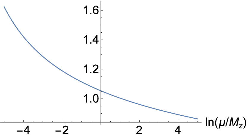
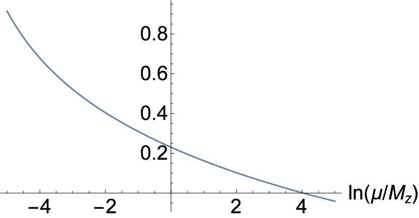
As a result, we obtained the unique solution (see Fig. 1) for the composite Higgs-boson model (1) or (13) as well as at the energy scale
| (18) |
and effective quartic coupling vanishes . As shown in Fig. 1, or the Fig. 2 in Ref. [12], our solution shows the following three important features. (I) The squared Higgs-boson mass changes its sign at , indicating the second-order phase transition from the SSB phase to the gauge symmetric phase for strong four-fermion coupling [13]. (II) The form-factor shows that the tightly bound composite Higgs particle behaves as if an elementary particle for . Recall that in the BHL analysis and are demanded for different values. (III) The effective form-factor of the composite Higgs boson is finite, indicating the formation of massive composite fermions ) in the gauge symmetric phase [13]. This critical point of the phase transition could be a ultra-violet (UV) fixed point for defining an effective gauge-symmetric field theory for massive composite fermions and bosons at TeV scales [12], and there are some possible experimental implications [19]. We do not address this issue in this article.
IV.3 Compare and contrast
It is important to compare and contrast our study with the BHL one [7]. In both studies, the definitions of all physical quantities are identical, the same RG equations (15) and (16) are used for the running Yukawa and quartic couplings as well as gauge couplings. However, the different boundary conditions are adopted. We impose the infrared boundary conditions (17) that are known nowadays, to uniquely determine the solutions of the RG equations, the values of the form-factor and high-energy scale . As shown in Fig. 1, [] monotonically increases (decreases) as the energy scale increases up to . Both experimental and values were unknown in the early 1990s, in order to find low-energy values and close to the IR-stable fixed point, BHL [7] imposed the compositeness conditions and for different values of the high-energy cutoff as the boundary condition to solve the RG equations. As a result, too large and values (Table I in Ref. [7]) were obtained, and we have reproduced these values. However, these BHL results are radically different from the present results of Eqs. (17), (18) and Fig. 1, showing that the composite Higgs boson actually becomes a more and more tightly bound state, as the energy scale increases, and eventually combines with an elementary fermion to form a composite fermion in the symmetric phase. This phase transition to the gauge symmetric phase is also indicated by as at which the 1PI vertex function in Eqs. (14) and (13) vanishes.
On the other hand, we compare and contrast our result with the study of the fundamental scalar theory for the elementary Higgs particle. The study of the high-order corrections to the RG equations of elementary Higgs quartic coupling “” and measured Higgs mass shows that becomes very small and smoothly varies in high energies approaching the Planck scale [21]. This is a crucial result for the elementary Higgs-boson model. This result is clearly distinct from the intermediate energy scale TeV obtained in the composite Higgs-boson model, where the quadratic term is removed by the mass gap equation of the SSB and an “unconventional” renormalization for the form factor of composite Higgs field is adopted [7]. Instead in the calculations of high-order corrections to the RG equations of the elementary Higgs quartic coupling “”, the quadratic term is removed in the prescription of the conventional renormalization for elementary scalar fields. It is worthwhile to mention that in Ref. [22] it is shown in the elementary Higgs-boson model that the quadratic term from high-order quantum corrections has a physical impact on the SSB and the phase transition to a symmetric phase occurs at the scale of order of TeV. Apart from described and discussed above, the effective four-fermion interaction theory has different dynamics from the fundamental scalar theory for the elementary Higgs particle, in particular for strong four-fermion coupling , e.g. the formations of boson and fermion bound states [13]. Nevertheless, all these studies of either the elementary or the composite Higgs-boson model play an important role in understanding new physics beyond the SM for fundamental particles.
V Origins of explicit symmetry breaking
Once the top-quark mass is generated via the SSB, other fermion masses are generated by the ESB via quark-lepton interactions and -boson vectorlike coupling.
V.1 Quark-lepton interactions
Although the four-fermion operators in Eq. (7) do not have quark-lepton interactions, we consider the following SM gauge-symmetric four-fermion operators that contain quark-lepton interactions [23],
| (19) |
where and for the third family. The “terms” represent for the first and second families with substitutions: , , and and . These operators (19) should be expected in the framework of Einstein-Cartan theory and unification theory [24]. Once the top quark mass is generated by the SSB, the quark-lepton interactions (19) introduce the ESB terms to the SD equations (mass-gap equations) for other fermions.
In order to show these ESB terms, we first approximate the SD equations to be self-consistent mass gap-equations by neglecting perturbative gauge interactions and using the large -expansion to the leading order, as indicated by Fig. 2. The quark-lepton interactions (19), via the tadpole diagrams in Fig. 2, contribute to the tau lepton mass and tau neutrino mass , provided the bottom-quark mass and top-quark mass are not zero. The latter is generated by the SSB, see Sec. IV. The former is generated by the ESB due to the -boson vectorlike coupling and top-quark mass , see next Sec. V.2. The superscript “sb” indicates the mass generated by the SSB. The superscript “eb” indicates the mass generated by the ESB. These are bare fermion masses at the energy scale .
Corresponding to the tadpole diagrams in Fig. 2, the mass-gap equations of tau lepton and tau neutrino are given by
| (20) | |||||
| (21) |
Here we use the self-consistent mass-gap equations of the bottom and top quarks [see Eq. (2.1) and (2.2) in Ref. [7]]
| (22) | |||||
| (23) |
and the definitions of Dirac quark, lepton and neutrino bare masses in general read
| (24) | |||||
| (25) |
and . The notation does not represent new SSB condensates, but the 1PI functions of fermion mass operator , i.e., the self-energy functions that satisfy the self-consistent SD equations or mass-gap equations. It is important to note the difference that Eq. (23) is the mass-gap equation for the top-quark mass generated by the SSB, while Eq. (23) is just a self-consistent mass-gap equation for the bottom-quark mass , as given by the tadpole diagram. The tau-neutrino mass and tau-lepton mass are not zero, if the top-quark mass and bottom-quark mass are not zero. This is meant to the mass generation of tau neutrino and tau lepton due to the ESB terms introduced by the quark-lepton interactions (19), quark masses and . It will be further clarified that these ESB terms are actually the inhomogeneous terms in the SD equations, which have nontrivial massive solutions without extra Goldstone bosons produced. In next section, we are going to show the other type of ESB term due to the -boson vectorlike coupling, that is crucial to have the bottom-quark mass generated by the ESB, once the top-quark mass is generated by the SSB.

V.2 -boson coupling to right-handed fermions
In addition to the ESB terms due to quark-lepton interactions, the effective vertex of -boson coupling to right-handed fermions at the energy scale also introduces the ESB terms to the Schwinger-Dyson equations for other fermions, once the top-quark mass is generated by the SSB. We study this effective vertex in this section.
In the low-energy SM obeying chiral gauge symmetries, the parity symmetry is violated, in particular, the -boson couples only to the left-handed fermions, i.e., . In order to show that the four-fermion operators (7) induce a 1PI vertex function of -boson coupling to the right-handed fermions, see Fig. 3, we take the third quark family in Eq. (10)
| (26) |
as an example for calculations. The leading contribution to the nontrivial 1PI vertex function is given by
| (27) | |||||
| (28) | |||||
| (29) |
where two fields in brackets in the line (27) mean the contraction of them, as shown in Fig. 3, the color degrees () of freedom have been summed and spinor indexes are explicitly shown in the line (28). represents the effective vertex function of -boson coupling to the right-handed fermions and ,
| (30) | |||||
Based on the Lorentz invariance, the 1PI vertex can be written as
| (31) |
where is the dimensionless Lorentz scalar. Beside, this vertex function (31) remains the same for exchanging and . The same calculations can be done by replacing and , as well as and .
As shown in Fig. 3 and Eq. (31), the two-loop calculation to obtain the finite part of the dimensionless Lorentz scalar is not an easy task. Nevertheless we can preliminarily infer its behavior as a function of energy and . For the case and , the vertex function vanishes in the IR domain of IR-fixed point of weak four-fermion coupling [7], where the SM with parity-violating gauge couplings of and bosons are realized. For the case and , increases as and increase. In addition the four-fermion coupling increases its strength as energy scale increases, i.e., the -function is positive [12]. This implies that in high energies and/or , the vertex function does not vanish and the -boson coupling to fermions is no longer purely left handed. On the other hand, at high-energy scale, the dependence of the vertex function on fermion masses is negligible, and is approximately universal for all quarks and leptons.

VI Schwinger-Dyson equations
After discussing the simplest mass-gap equations (20) and (23) and the effective -boson coupling vertex (31), we turn to the SD equations for fermion self-energy functions by taking gauge interactions into account. It is known that in the SM the boson does not contribute to the SD equations for fermion self-energy functions . However, due to the nontrivial vertex function (31), the gauge boson has the contribution, as shown in Fig. 4, to SD equations at high energies. This contribution not only introduces an explicit symmetry breaking term, but also mixes up SD equations for self-energy functions of different fermion fields via the CKM mixing matrix [23, 25].
In the vectorlike gauge theory, SD equations for fermion self-energy functions were intensively studied in Ref. [26]. In the Landau gauge, SD equations for and quarks are given by
| (32) | |||||
| (33) |
where the integration is up to the cutoff , and are the vertex functions of vectorlike gauge theories. In Eq. (32), the bare mass term comes from the SSB, see the simplest mass-gap equation (23) and discussions in Sec. IV. Instead, the bare mass term in Eq. (33) comes from the ESB terms due to the effective -boson coupling vertex (31) and the self-consistent mass-gap equation (22). We neglect corrections to vertex functions of vectorlike gauge interactions, for example, and in the QED case. Since the vertex function in Eq. (31) does not vanish only for high energies, we approximately treat it as a boundary value at the scale
| (34) |
where . This means that the contributions of Fig. 4 are approximately boundary terms in the integral SD equations (32) and (33), see the following equations (35)-(38). Thus we neglect possible right-handed couplings of the would-be Nambu-Goldstone bosons in the Landau gauge, which could have effects on the explicit gauge symmetry breaking. In the future we will study these effects in some more detail.
Following the approach of Ref. [26], we convert Eqs. (32) and (33) to the following boundary value problems (, ):
| (35) | |||
| (36) |
and
| (37) | |||
| (38) |
The boundary conditions (36) and (38) are actually the mass-gap equations of and quarks at the scale , the -terms come from the contribution of Fig. 4, - and -terms come from Eqs. (22) and (23). Analogously, we obtain the following boundary value problem for the and leptons:
| (39) | |||||
| (40) |
and
| (41) | |||||
| (42) |
where is the element of PMNS mixing matrix. The boundary conditions (40) and (42) are actually the mass-gap equations of and leptons at the scale , the -terms come from the contribution of Fig. 4, - and -terms come from Eqs. (21) and (20). In the rhs of self-consistent mass-gap equations (36), (38), (40) and (42), only the top-quark mass term is due to the SSB, see Eq. (20) and Sec. IV, whereas the -terms are the ESB terms due to the effective vertex (31), see Fig. 4, whereas the -, - and -terms are ESB terms, satisfying the self-consistent mass-gap equations, e.g., Eqs. (21)-(23) due to the quark-lepton interactions (19), four-fermion interactions (10) and (12). All ESB terms are functions of the top-quark mass term , which is the unique origin of the ESB terms. The SD equations (35(-(42) are coupled, become inhomogeneous and we try to find the nontrivial massive solutions for the bottom quark, tau lepton and tau neutrino.
Suppose that the SSB for the top-quark mass does not occur (), fermion bare masses are zero and the -boson contribution vanishes (). In this case the SD equations (35-42) are homogenous. It was established [26] that only trivial solutions to homogeneous SD equations exist in the weak coupling phase , however, inhomogeneous SD equations have nontrivial solutions
| (43) |
where the factor comes from the corrections of perturbative gauge interactions and is the anomalous dimension of fermion mass operators. Actually, when and the nonlinearity in SD equations is neglected, Eqs. (35), (37) and (41) admit the solution [27],
| (44) |
“”, and is the infrared scale. In Eqs. (43) and (44), the infrared mass scales are proportional to the inhomogeneous terms attributed to the ESB terms, which are in our scenario -terms and mass terms . Equation (39) for -neutrino () admits the solution that is related to the inhomogeneous term of the ESB at the infrared scale .

VII The masses of third fermion family
First we try to find the massive solutions () to the mass-gap equations Eqs. (36), (38), (40) and (42) at the energy scale . In these equations, the term can be neglected, since , where Eq. (43) is used. We define the bare masses , , , and . As a result, we approximately obtain
| (45) | |||||
| (46) | |||||
| (47) | |||||
| (48) |
where [28] and . Equations (45) and (47) are used in the last inequality of Eq. (46). Equations (45)-(48) show that at the energy scale , the ESB masses , and are originated from the SSB mass . The last step in Eqs. (45-48) shows the dominate contributions: (i) the -neutrino acquires its mass from the -quark mass via the quark-lepton interaction (19), (ii) the -quark acquires its mass from the -quark mass via the CKM mixing, (iii) the -lepton acquires its mass from the bottom-quark mass via the quark-lepton interaction (19) and -neutrino mass via the PMNS mixing. In this article, we only indicate that the tau neutrino Dirac mass relates to the top-quark mass without further discussions, since the problem of neutrinos masses is complex for their Dirac or Majorana feature. We will discuss in the future that the Dirac mass of the left-handed neutrino and right-handed sterile neutrino , as well as the large Majorana mass of Majorana neutrino ) generated by the four-fermion operator in Eq. (7), in order to see if the smallness of gauged Majorana neutrino masses is consistent with experimental data.
In order to find the fermion self-energy function (43) or (44) at the infrared mass scale , we need to solve the inhomogeneous SD equations (35), (37) and (41) with the boundary values (45)-(48). This is still a difficult task. To the leading order, neglecting the corrections from perturbative gauge interactions, we use Eqs. (46) and (48) to approximately obtain the bottom quark and -lepton masses at the infrared mass scale ,
| (49) |
in terms of the top-quark mass , and we define the bottom-quark and tau-lepton Yukawa couplings
| (50) |
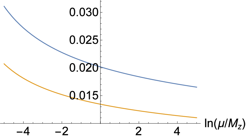
which are obviously related to the top-quark Yukawa coupling . In Fig. 5, the Yukawa couplings and are plotted. Comparing them with the Yukawa coupling in Fig. 1, one finds the hierarchy pattern of the Yukawa couplings in the third fermion family.
Using the top-quark mass-shell condition and experimental values of top- and bottom-quark masses: GeV and GeV, as well as the gauge-coupling value , we numerically obtain the - and -values at the energy scale ,
| (51) |
and in Eq. (34). Note that in Fig. 1 has received the contributions from the renormalized gauge couplings of the SM, see Sec. IV. Thus we approximately determine the finite part of vertex function (31), since we have not calculated it.
In the determination of the -lepton mass, we take into account the corrections of perturbative gauge interactions by adopting the RG solutions for fermion masses [29] (the number of quark flavors ),
| (52) |
and . We use Eqs. (49), (50), (52) and the -lepton mass-shell condition
| (53) |
to uniquely determine the -lepton mass GeV. This is a qualitative result, since we have only considered in the inhomogeneous SD equation the possible dominate contributions to the tau lepton mass and neglected other contributions, e.g., the fermion-family mixing. Nevertheless, the result is in a qualitative agreement with the experimental value GeV, and consistently shows the hierarchy spectrum of fermion masses , and in the third family. It should be emphasized that these qualitative results cannot to be quantitatively compared with the SM precision tests. The quantitative study is a difficult and challenging task and one will probably be able to carry it out by using a numerical approach in the future.
VIII A brief conclusion and some remarks
Our goal in this article is to present a possible scenario and understanding of the origins and hierarchy spectrum of fermion masses in the third family of the SM. We obtain the fermion masses, Yukawa couplings and their relations, as well as the energy scale TeV at which the second-order phase transition occurs from the SSB phase to the gauge symmetric phase. All these results are preliminarily qualitative, and they should receive the high-order corrections and some nonperturbative contributions. Nevertheless, these results may give us some insight into the long-standing problem of fermion-mass origin and hierarchy. We will present the similar study including the first and second families, as well as neutrinos by taking into account the fermion-family mixing to understand the hierarchy spectrum of SM fermions: from top quark to electron neutrino [30]. It is much more complicated to solve the SD equations for the SM fermion masses, however, the basic scenario is simply the same. Due to the ground-state (vacuum) alignment of the effective theory of relevant operators, the top-quark mass is generated by the SSB, and other fermion masses are originated from the ESB terms, which are induced by the top-quark mass via the fermion-family mixing, quark-lepton interactions and vectorlike -boson coupling at high energies. As a consequence, fermion Yukawa couplings are functions of the top-quark Yukawa coupling.
In this article, the top-quark Yukawa coupling in fact relates to the nonvanishing form-factor of composite Higgs boson, see Eq. (14). Both of them, as shown in Fig. 1, are of the order of unity and slowly vary from GeV to TeV. This means that the composite Higgs boson is a tightly bound state, as if an elementary Higgs boson. In addition, relating to the top-quark Yukawa coupling , the Yukawa couplings and also slowly vary from GeV to TeV, see Fig. 5. These features imply that it should be hard to have any detectable nonresonant signatures in the LHC -collisions, showing the deviations from the SM with the elementary Higgs boson.
To end this article, we would like to mention that the vectorlike feature of -boson coupling at high energy is expected to have some collider signatures on the decay channels of -boson into both left- and right-handed helicity states of two high-energy leptons or quarks. The branching ratios of different helicity states are expected to be almost the same, given the qualitative estimation of Eqs. (34) and (51). This contrasts to the helicity suppression in the low-energy SM due to its -boson coupling being purely left handed, recalling the helicity suppression of pion decay into an electron and the corresponding electron antineutrino. On the other hand, the forward-backward asymmetry in top-quark pair production measured by the CDF [31] and D0 [32] at the Fermilab Tevatron collisions seems to be larger than the SM (QCD) result. This may be related to the vectorlike (parity-restoration) feature of -boson coupling at high energy, since the top-quark pair can be produced by , and quarks in the -channel via the -boson exchange. We will study it in detail.
IX Acknowledgments
The author thanks the anonymous referee for his/her effort of reviewing this article. The author thanks Professor Hagen Kleinert for discussions on the domains of IR- and UV-fixed points of gauge field theories, and to Professor Zhiqing Zhang for discussions on the experimental physics in the LHC.
References
- [1] Y. Nambu and G. Jona-Lasinio, Phys. Rev. 122 (1961) 345.
- [2]
F. Englert, R. Brout, Phys. Rev. Lett. 13 (1964) 321;
P. W. Higgs, Phys. Lett. 12 (1964) 132; Phys. Rev. Lett. 13 (1964) 508; Phys. Rev. 145 (1966) 1156;
G. S. Guralnik, C. R. Hagen, T. W. B. Kibble, Phys. Rev. Lett. 13 (1964) 585; T. W. B. Kibble, Phys. Rev. 155 (1967) 1554. - [3]
ATLAS Collaboration, Phys. Lett. B 716 (2012) 1;
CMS Collaboration, Phys. Lett. B 716 (2012) 30-61. - [4]
CDF Collaboration, Phys. Rev. Lett. 74, 2626
(1995);
D0 Collaboration, Phys. Rev. Lett. 74, 2422 (1995). - [5] C. T. Hill, Phys. Lett. B266 (1991) 491 and ibid B345 (1995) 483; Phys. Rev. D87 (2013) 065002.
- [6] C. T. Hill, Phys. Rev. D24, 691 (1990); C. T. Hill, C. N. Leung, S. Rao, Nucl. Phys. B262, 517, (1985); J. Bagger, S. Dimopoulous, E. Masso, Phys. Rev. Lett. 55 920 (1985).
- [7] W. A. Bardeen, C. T. Hill and M. Lindner, Phys. Rev. D41 (1990) 1647.
- [8]
Y. Nambu, in Proceedings of
the 1989 Workshop on Dynamical Symmetry Breaking, edited
by T. Muta and K. Yamawaki (Nagoya University, Nagoya, Japan, 1990);
V.A. Miranski, M. Tanabashi and K. Yamawaki, Mod. Phys. Lett. A4 (1989) 1043; Phys. Lett. B221 (1989) 117;
H. Kleinert, the SU(3)-extension of their work in Chapter 26 of the textbook http://klnrt.de/b6, ”Particles an Quantum Field” World Scientific Publishing Company, 2016. - [9] W. J. Marciano, Phys. Rev. Lett. 62, (1989) 2793.
- [10]
G. Cvetic, Rev. Mod. Phys. 71 (1999) 513-574;
C. T. Hill, E. H. Simmons, Phys. Rept. 381 (2003) 235-402; Erratum-ibid. 390 (2004) 553-554. - [11] S.-S. Xue, Phys. Lett. B727 (2013) 308.
- [12] S.-S. Xue, Phys. Lett. B737 (2014) 172.
- [13] S.-S. Xue, Phys. Lett. B381 (1996) 277, Nucl. Phys. B486 (1997) 282, ibid B580 (2000) 365, Phys. Rev. D 61 (2000) 054502, ibid D64 (2001) 094504, J. Phys. G, Nucl. Part. Phys. 29 (2003) 2381.
- [14] ATLAS Collaboration, J. High Energy Phys. 12 (2015)055, arXiv:1506.00962.
- [15] CMS Collaboration, Phys. Rev. D91, 052009 (2015), arXiv:1501.04198
- [16] S.-S. Xue, Phys. Rev. D82, 064039 (2010), Phys. Lett. B682 (2009) 300 and ibid B711 (2012) 404.
- [17] H.B. Nielson and M. Ninomiya, Nucl. Phys. B185 (1981) 20, ibid B193 (1981) 173, Phys. Lett. B105 (1981) 219, Int. J. Mod. Phys. A6 (1991) 2913.
- [18] see for example, C. Itzykson and J-B. Zuber “Quantum Feild Theory” page 161, McGraw-Hill, Inc. ISBN 0-07-032071-3.
- [19] S.-S. Xue, Phys. Lett. B744 (2015) 88–94.
- [20] S.-S. Xue, Phys. Lett. B721 (2013) 347.
- [21] see for example, D. Buttazzo, G. Degrassi, P. P. Giardino, G. F. Giudice, et al., JHEP 12 (2013), 089.
- [22] D. Bai, J.-W. Cui, Y.-L. Wu, Phys. Lett. B746 (2015) 379–384.
- [23] S.-S. Xue, Modern Physics Letters A, Vol. 14 (1999) 2701.
- [24]
E. Eichten, J. Preskill, Nucl. Phys. B 268 (1986) 179;
M. Creutz, C. Rebbi, M. Tytgat, S.-S. Xue, Phys. Lett. B 402 (1997) 341. - [25] S.-S. Xue, Phys. Lett. B398 (1997) 177.
- [26]
R. Fukuda and T. Kugo, Nucl. Phys. B117 (1976) 250,
W.A. Bardeen, C.N. Leung, and S.T. Love, Nucl. Phys. B273 (1986) 649; ibid B323 (1989) 493.
A. Kocić, S. Hands, B. Kogut and E. Dagotto, Nucl. Phys. B347 (1990) 217.
G. Preparata and S.-S. Xue, Phys. Lett. B264, (1991) 35, ibid B302 (1993) 442, B325 (1994) 161. - [27] S.-S. Xue, Modern Physics Letters A, Vol. 15 (2000) 1089.
- [28] J. Beringer et al. (Particle Data Group Collaboration), Phys. Rev. D 86, 010001 (2012).
- [29] See for example, “Gauge theory of elementray particle physics” by T. P. Cheng and L. F. Li, Oxford University Press Inc. New York, 1984, ISBN 978-019-851961-4 (page 449), the references therein.
- [30] S.-S. Xue, in preparation.
- [31] CDF collaboration, Phys. Rev. Lett. 101, 202001.
- [32] D0 collaboration, Phys. Rev. Lett. 100, 142002.