On the stationary Navier-Stokes
equations in the half-plane

Julien Guillod and Peter Wittwer
Department of Theoretical Physics,
University of Geneva, Switzerland

Abstract

We consider the stationary incompressible Navier-Stokes equation in the half-plane with inhomogeneous boundary condition. We prove existence of strong solutions for boundary data close to any Jeffery-Hamel solution with small flux evaluated on the boundary. The perturbation of the Jeffery-Hamel solution on the boundary has to satisfy a nonlinear compatibility condition which corresponds to the integral of the velocity field on the boundary. The first component of this integral is the flux which is an invariant quantity, but the second, called the asymmetry, is not invariant, which leads to one compatibility condition. Finally, we prove existence of weak solutions, as well as weak-strong uniqueness for small data.

Keywords: Navier-Stokes equations, Flow-structure interactions, Jeffery-Hamel flow
MSC class: 76D03, 76D05, 35Q30, 76D25, 74F10, 76M10

1 Introduction

The stationary and incompressible Navier-Stokes equations in the half-plane

\Omega=\left\{(x,y)\in\mathbb{R}^{2}\colon y>1\right\}

are

	$\displaystyle\Delta\boldsymbol{u}-\boldsymbol{\nabla}p$	$\displaystyle=\boldsymbol{u}\boldsymbol{\cdot}\boldsymbol{\nabla}\boldsymbol{u}\,,$	$\displaystyle\boldsymbol{\nabla}\boldsymbol{\cdot}\boldsymbol{u}$	$\displaystyle=0\,,$		(1)
	$\displaystyle\left.\boldsymbol{u}\right\|_{\partial\Omega}$	$\displaystyle=\boldsymbol{u}^{*}\,,$	$\displaystyle\lim_{\|\boldsymbol{x}\|\to\infty}\boldsymbol{u}$	$\displaystyle=\boldsymbol{0}\,,$		(1)

where $\boldsymbol{u}^{*}$ is a boundary condition. Due to the incompressibility of the fluid, the flux is an invariant quantity,

\Phi=\int_{\partial\Omega}\boldsymbol{u}^{*}\boldsymbol{\cdot}\boldsymbol{n}=\int_{\mathbb{R}}v(x,y)\,\mathrm{d}x\,,

for all $y\geq 1$ , where $\boldsymbol{u}=(u,v)$ and $\boldsymbol{n}=(0,1)$ is the normal vector to the half-plane. This problem (see \figrefschemea) presents three difficulties: $\Omega$ is a two-dimensional unbounded domain, the boundary of $\partial\Omega$ is unbounded, and the boundary data are not zero. There is not much previous work on this problem, but some authors have treated related problems. Concerning the half-plane problem, Heywood (1976, §5) proves the uniqueness of solutions for the steady Stokes equation and the time-dependent Navier-Stokes equation. The so called Leray’s problem, which consists of a finite number of outlets connected to a compact domain, has been studied in detail by Amick (1977); Amick (1978); Amick (1980) and several other authors, but the resolvability for large fluxes is still an open problem. Fraenkel (1962); Fraenkel (1963) provides a formal asymptotic expansion of the stream function in case of a curved channel by starting with the Jeffery-Hamel solution (Jeffery, 1915; Hamel, 1917) for the first order. The case of paraboloidal outlets was first treated by Nazarov & Pileckas (1998), and then more recently by Kaulakytė & Pileckas (2012); Kaulakytė (2013). Another important class of similar problems are the aperture domains, introduced by Heywood (1976), as shown in \figrefschemeb. The linear approximation was studied in any dimension by Farwig (1996); Farwig & Sohr (1996). The three-dimensional case was treated by Borchers & Pileckas (1992), as well as other authors. For the two-dimensional nonlinear problem, Galdi et al. (1995) proved that the velocity tends to zero in the $L^{2}$ -norm for arbitrary values of the flux. For small fluxes, Galdi et al. (1996) and Nazarov (1996) show that the asymptotic behavior is given by a Jeffery-Hamel solution but only if the problem is symmetry with respect to the $y$ -axis. The asymptotic behavior of the two-dimensional aperture problem in the nonsymmetric case is still open. Finally, Nazarov et al. (2001); Nazarov et al. (2002) considered a straight channel connected to a half-plane (see \figrefschemec), and looked under which conditions the asymptotic behavior is given by a Jeffery-Hamel flow in the half-plane and by the Poiseuille flow in the channel. Theses conditions are described in details later on. On a more applied side, the bifurcation properties and the stability of the Jeffery-Hamel flows have retained the attention of many authors (Moffatt & Duffy, 1980; Sobey & Drazin, 1986; Banks et al., 1988; Uribe et al., 1997; Drazin, 1999).

Figure 1: (a) The domain

\Omega

we consider is the half plane defined by

x\in\mathbb{R}

and

y>1

; (b) an aperture domain; (c) a channel connected to a half-plane.

Jeffery-Hamel flows play an important role in the asymptotic behavior of flows carrying flux. They own their name to the work of Jeffery (1915); Hamel (1917), and are radial scale invariant solutions of the two-dimensional stationary incompressible Navier-Stokes equations

\displaystyle\Delta\boldsymbol{u}-\left(\boldsymbol{u}\boldsymbol{\cdot}\boldsymbol{\nabla}\right)\boldsymbol{u}-\boldsymbol{\nabla}p

\displaystyle=\boldsymbol{0}\,,

\displaystyle\boldsymbol{\nabla}\boldsymbol{\cdot}\boldsymbol{u}

\displaystyle=0\,,

in domains

D=\left\{\left(r\sin(\theta),r\cos(\theta)\right)\in\mathbb{R}^{2}\colon\,r>0\text{ and }\theta\in\left(-\beta,\beta\right)\right\}

with $\beta\in\bigl(0,\tfrac{\pi}{2}\bigr]$ , satisfying the boundary condition

\boldsymbol{u}\bigr|_{\partial D\setminus\left\{\boldsymbol{0}\right\}}=\boldsymbol{0}\,.

Explicitly, a Jeffery-Hamel solution $\boldsymbol{u}_{\textsc{jh}}$ is of the form

\boldsymbol{u}_{\textsc{jh}}(r,\theta)=\dfrac{1}{r}f(\theta)\,\boldsymbol{e}_{r}\,,

with $f$ a solution of the nonlinear second order ordinary differential equation

f^{\prime\prime}+f^{2}+4f=2C\,,

with $C\in\mathbb{R}$ , satisfying the boundary condition $f(\pm\beta)=0$ . The constant $C$ is related to the flux $\Phi$ of the flow,

\Phi=\int_{-\beta}^{+\beta}f(\theta)\,\mathrm{d}\theta\,.

The Jeffery-Hamel solutions have been intensively studied (Rosenhead, 1940; Fraenkel, 1962; Banks et al., 1988; Tutty, 1996), and, because some mathematical questions still remain open, there has been a regain of interest in recent years (Rivkind & Solonnikov, 2000; Kerswell et al., 2004; Putkaradze & Vorobieff, 2006; Corless & Assefa, 2007).

In what follows we are interested in the half-plane case, so we consider $\beta=\tfrac{\pi}{2}$ , i.e., when the domain is the upper half plane $D=\mathbb{R}\times\left(0,\infty\right)$ . In Cartesian coordinates, the two components of the velocity of the Jeffery-Hamel solutions are

\displaystyle u_{\textsc{jh}}(x,y)

\displaystyle=\frac{1}{y}f_{u}\left(\frac{x}{y}\right)\,,

\displaystyle v_{\textsc{jh}}(x,y)=

\displaystyle\frac{1}{y}f_{v}\left(\frac{x}{y}\right)\,,

(2)

with

\displaystyle f_{u}(s)

\displaystyle=\frac{s\,f(\arctan s)}{1+s^{2}}\,,

\displaystyle f_{v}(s)

\displaystyle=\frac{f(\arctan s)}{1+s^{2}}\,.

Figure 2: Existence of the Jeffery-Hamel flows for small values of the flux

\Phi

. For

\Phi>0

, there exists one symmetric solutions, but for

\Phi<0

, also two additional asymmetric solutions exist.

The Jeffery-Hamel solutions for $\beta=\tfrac{\pi}{2}$ have a peculiar property: for small $\Phi<0$ there is more than one solution. In fact, as shown in appendix §A, $\Phi=0$ is a tri-critical bifurcation point, see \figrefbifurcation-JH. For small $\Phi>0$ the Jeffery-Hamel problem has a solution $\boldsymbol{u}_{\Phi}^{0}$ which is symmetric with respect to the $y$ -axis. The solution $\boldsymbol{u}_{\Phi}^{0}$ also exists for small values of $\Phi<0$ , but when crossing from $\Phi>0$ to $\Phi<0$ , an additional pair $\boldsymbol{u}_{\Phi}^{\pm 1}$ of asymmetric solutions (related to each other by a reflection with respect to the $y$ -axis) appears. For $\Phi=0$ , the Jeffery-Hamel solution is the zero function, and will be ignored in what follows.

The central idea of the method we use to study (), is to interpret the system as an evolution equation with $y$ playing the role of time. The boundary data of the original problem then become the initial data for the resulting Cauchy problem. This allows discussing the “time” dependence of quantities like the flux $\Phi=\int_{\mathbb{R}}v(x,y)\mathrm{d}x$ and the asymmetry $A=\int_{\mathbb{R}}u(x,y)\mathrm{d}x$ in a natural setting. We assume for the moment sufficient decay for these integrals to make sense. As can be seen from (), the flux and the asymmetry are invariants for a Jeffery-Hamel solution $\boldsymbol{u}_{\Phi}^{\sigma}$ , i.e., they are independent of the time $y$ , and therefore

	$\displaystyle A$	$\displaystyle=\int_{\mathbb{R}}u_{\Phi}^{\sigma}(x,1)\,\mathrm{d}x=\int_{\mathbb{R}}u_{\Phi}^{\sigma}(x,y)\,\mathrm{d}x=\lim_{y\rightarrow\infty}\int_{\mathbb{R}}u_{\Phi}^{\sigma}(x,y)\,\mathrm{d}x\,,$
	$\displaystyle\Phi$	$\displaystyle=\int_{\mathbb{R}}v_{\Phi}^{\sigma}(x,1)\,\mathrm{d}x=\int_{\mathbb{R}}v_{\Phi}^{\sigma}(x,y)\,\mathrm{d}x=\lim_{y\rightarrow\infty}\int_{\mathbb{R}}v_{\Phi}^{\sigma}(x,y)\,\mathrm{d}x\,.$

The flux is an invariant of the Navier-Stokes equation (), i.e., if $\boldsymbol{u}$ is a solution of the Navier-Stokes equation, then for $y>1$ ,

\int_{\mathbb{R}}v(x,1)\,\mathrm{d}x=\int_{\mathbb{R}}v(x,y)\,\mathrm{d}x=\lim_{y\rightarrow\infty}\int_{\mathbb{R}}v(x,y)\,\mathrm{d}x\,,

but the asymmetry is not an invariant, so typically,

\int_{\mathbb{R}}u(x,1)\,\mathrm{d}x\neq\int_{\mathbb{R}}u(x,y)\,\mathrm{d}x\neq\lim_{y\rightarrow\infty}\int_{\mathbb{R}}u(x,y)\,\mathrm{d}x\,.

As we will see below, for solutions that are close but not equal to Jeffery-Hamel, the asymmetry is no more an invariant, and this fact is the main source of trouble for the construction of solutions.

Jeffery-Hamel solutions are singular at the origin, and, in order to study this phenomenon, i.e. look for solutions which are close to Jeffery-Hamel flows, it is necessary to regularize the problem. For this purpose, given a Jeffery-Hamel solution $\boldsymbol{u}_{\Phi}^{\sigma}$ in the upper half plane $D=\left\{(x,y)\in\mathbb{R}^{2}\colon y>0\right\}$ , we restrict it to the domain $\Omega=\left\{(x,y)\in\mathbb{R}^{2}\colon y>1\right\}$ , and construct stationary solutions of the Navier-Stokes equations which are close to the Jeffery-Hamel flow by imposing boundary conditions of the form

\boldsymbol{u}\bigr|_{\partial\Omega}=\boldsymbol{u}_{\Phi}^{\sigma}\bigr|_{\partial\Omega}+\boldsymbol{u}_{b}\,,

(3)

with $\boldsymbol{u}_{b}$ small and with zero flux,

\int_{\partial\Omega}\boldsymbol{u}_{b}\boldsymbol{\cdot}\boldsymbol{n}=0\,.

Even when considering such boundary conditions, we are not able to perform a fixed point argument on the nonlinearity by inverting the Stokes problem. The main reason is that the flux is determined by the boundary condition, while the asymmetry is not. In order to adjust the asymmetry, we rewrite the boundary condition as

\left.\boldsymbol{u}\right|_{\partial\Omega}=\left.\boldsymbol{u}_{\Phi}^{\sigma}\right|_{\partial\Omega}+\left(A,0\right)\frac{1}{\sqrt{2\pi}}\mathrm{e}^{-\frac{1}{2}x^{2}}+\boldsymbol{u}_{s}\,,

(4)

where

A=\int_{\mathbb{R}}u_{b}\,,

so that $\boldsymbol{u}_{s}$ has no asymmetry and no flux.

\int_{\mathbb{R}}\boldsymbol{u}_{s}=\boldsymbol{0}\,.

The choice of $\mathrm{e}^{-\frac{1}{2}x^{2}}$ in () is for convenience later on, and we could have chosen instead any other smooth function of rapid decay.

We will show the existence of strong solutions to the Navier-Stokes equation (), with the boundary condition () for $\Phi$ small and $\boldsymbol{u}_{s}$ in a small ball by adjusting the parameter $A$ . The main result is the following:

Theorem 1.

For all boundary condition of the form () with $\boldsymbol{u}_{\Phi}^{\sigma}$ a Jeffery-Hamel solution with small enough flux $\Phi$ and all $\boldsymbol{u}_{s}$ in a small enough neighborhood of zero in some function space, there exists a solution $(\boldsymbol{u},p)$ of the Navier-Stokes equation in $\Omega$ , satisfying

\lim_{y\rightarrow\infty}y\left(\sup_{x\in\mathbb{R}}\bigl|\boldsymbol{u}-\boldsymbol{u}_{\Phi}^{\sigma}\bigr|\right)=0\,,

and

\displaystyle\begin{aligned} \boldsymbol{\nabla}\boldsymbol{u}&\in L^{2}(\Omega)\,,\\ \boldsymbol{u}/y&\in L^{2}(\Omega)\,,\end{aligned}

\displaystyle\begin{aligned} y\boldsymbol{u}&\in L^{\infty}(\Omega)\,,\\ y^{2}\boldsymbol{\nabla}\boldsymbol{u}&\in L^{\infty}(\Omega)\,.\end{aligned}

(5)

Moreover, if $\boldsymbol{v}$ is a weak solution (defined in ()) of () and $\boldsymbol{u}$ a strong solution of () satisfying (), then $\boldsymbol{u}=\boldsymbol{v}$ , provided $\boldsymbol{u}^{*}$ is small enough.

We now discuss more precisely the results of Nazarov et al. (2001); Nazarov et al. (2002), for the domain shown in \figrefschemec. We note that in this domain, the flux through the channel is not prescribed. They show that by requiring the asymptotic behavior to be an antisymmetric Jeffery-Hamel solution $\boldsymbol{u}_{\Phi}^{\pm 1}$ , there exists a unique solution in some weighted space, and the flux is uniquely determined by the data. Conversely, by requiring that the asymptotic behavior is given by a symmetric Jeffery-Hamel solution $\boldsymbol{u}_{\Phi}^{0}$ , the Navier-Stokes equation linearized around $\boldsymbol{u}_{\Phi}^{0}$ leads to a well-posed problem for $\Phi<0$ and to an ill-posed one for $\Phi>0$ . So for $\Phi<0$ , there exists a unique solution for all small enough fluxes, but for $\Phi>0$ , the asymptotic behavior is still unknown. So we believe that in case $\Phi<0$ , the Navier-Stokes equation in the half-plane () has a solution decaying like $r^{-1}$ at infinity whose asymptote is given by a Jeffery-Hamel solution, but in the case $\Phi>0$ , it is still not clear that the solution is in general bounded by $r^{-1}$ .

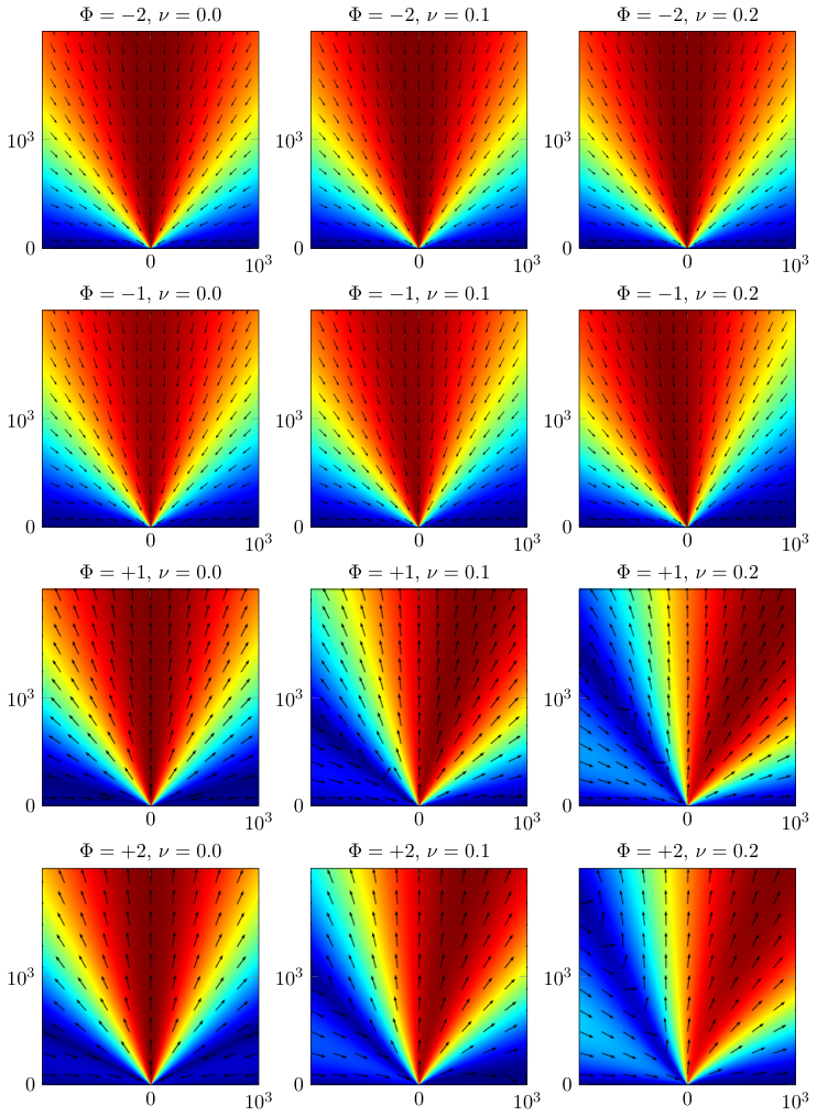
The remainder of this paper is organized as follows. In \secrefhalplane-spaces, we introduce the function spaces which we use for the mathematical formulation of the problem, and prove some basic bounds. In \secrefstokes, we rewrite the Stokes equation as a dynamical system, present the associated integral equations, and provide bounds on the solution of the Stokes system, so that in \secrefns, we can show the existence of strong solutions to the Navier-Stokes system. In \secrefweaksol, we prove existence of weak solutions, and, finally, in \secrefuniqueness, we prove uniqueness of solutions for small data with a weak-strong uniqueness result. In the last part, we also present numerical simulations that show that the asymptotic behavior is most likely not given by the Jeffery-Hamel solution if $\Phi>0$ . In the appendix, we show the existence of symmetric and asymmetric Jeffery-Hamel solutions with small flux.

2 Function spaces

As explained in the introduction, our strategy of proof is to rewrite () as a dynamical system with $y$ playing the role of time. This system is studied by taking the Fourier transform in the variable $x$ , which transforms the system into a set of ordinary differential equations with respect to $y$ . We now define the function spaces for the Fourier transforms of the velocity field, pressure field and the nonlinearity. The choice of spaces is motivated by the scaling property of the equations with respect to $x$ and $y$ when linearized around a Jeffery-Hamel solution. This setup turns out to be natural for the description of the asymptotic behavior of solutions close to Jeffery-Hamel flows. Similar function spaces were already used by Wittwer (2002), where the basic operations which are needed for the discussion of the Navier-Stokes equations were discussed. In particular, Wittwer (2002) shows basic bounds on the convolution with respect to the variable $k$ , the Fourier conjugate variable of $x$ , which is needed to implement the nonlinearities, and bounds on the convolution with the semigroup $\mathrm{e}^{-\left|k\right|y}$ which is associated with the Stokes operator when viewed as a time evolution in $y$ . Further properties and improved bounds have been proved by Hillairet & Wittwer (2009); Boeckle & Wittwer (2012).

Definition 2 (Fourier transform and convolution).

For two functions $\hat{f}$ and $\hat{g}$ defined almost everywhere in $\Omega$ and which are in $L^{1}(\mathbb{R})$ for all $y\geq 1$ , the inverse Fourier transform of $\hat{f}$ is defined by

f(x,y)=\mathcal{F}\bigl[\hat{f}\,\bigr](x,y)=\int_{\mathbb{R}}\mathrm{e}^{\mathrm{i}kx}\hat{f}(k,y)\,\mathrm{d}k\,,

and the convolution by

\bigl(\hat{f}*\hat{g}\bigr)(k,y)=\int_{\mathbb{R}}\hat{f}(k-\ell,y)\hat{g}(\ell,y)\,\mathrm{d}\ell\,.

We note that with these definitions,

fg=\mathcal{F}\bigl[\hat{f}*\hat{g}\bigr]\,.

We now define two families of function spaces: the first one is for functions of $k$ only which will be used for the boundary data, and the second one is for functions of $k$ and $y$ :

Definition 3 (function spaces on $\partial\Omega$ ).

For $\alpha\geq 0$ and $q\in\mathbb{R}$ , let $\mathcal{A}_{\alpha,q}$ be the Banach space of functions $\hat{f}\in C(X,\mathbb{C})$ where

X=\begin{cases}\mathbb{R}\,,&q\geq 0\,,\\ \mathbb{R}\setminus\{0\}\,,&q<0\,,\end{cases}

(6)

such that $\overline{\hat{f}(k)}=\hat{f}(-k)$ and such that the norm

\bigl\|\hat{f};\mathcal{A}_{\alpha,q}\bigr\|=\sup_{X}\frac{\bigl|\hat{f}\bigr|}{\eta_{\alpha,q}}\qquad\text{with}\qquad\eta_{\alpha,q}(k)=\frac{\left|k\right|^{q}}{1+\left|k\right|^{\alpha+q}}\,,

is finite. For $\alpha\geq 0$ and $q\geq 0$ , let $\mathcal{T}_{\alpha,q}$ and $\mathcal{W}_{\alpha,q}$ , be the Banach space of functions in $\mathcal{A}_{\alpha+1,\min(0,q-1)}$ such that their respective norm

\displaystyle\bigl\|\hat{f};\mathcal{T}_{\alpha,q}\bigr\|

\displaystyle=\sum_{i=0}^{\lfloor q\rfloor}\bigl\|\partial_{k}^{i}\hat{f};\mathcal{A}_{\alpha+1,\min(0,q-1-i)}\bigr\|\,,

\displaystyle\bigl\|\hat{f};\mathcal{W}_{\alpha,q}\bigr\|

\displaystyle=\sum_{i=0}^{\lfloor q\rfloor}\bigl\|\partial_{k}^{i}\hat{f};\mathcal{A}_{\alpha+1,q-1-i}\bigr\|\,,

is finite, where $\lfloor q\rfloor$ denotes the integer part of $q$ .

Remark 4.

The parameter $\alpha$ captures the behavior of functions at infinity, which corresponds to the regularity in $x$ in direct space. For example, if $\hat{f}\in\mathcal{A}_{\alpha,0}$ for $\alpha>1$ , then $\hat{f}\in L^{1}(\mathbb{R})$ and by the dominated convergence theorem, $f\in C(\mathbb{R})$ . The index $q$ characterizes the behavior near $k=0$ : a function which behaves like $\left|k\right|^{q}$ around zero is in the space $\mathcal{A}_{\alpha,q}$ . The space $\mathcal{T}_{\alpha,q}$ includes some characterization of the derivative with respect to $k$ , which is needed in order to characterized the behavior near $k=0$ as shown in the next lemma.

Lemma 5.

For all $\hat{f}\in\mathcal{T}_{\alpha,q}$ , the function

\hat{g}(k)=\hat{f}(k)-\left(\sum_{i=0}^{\lfloor q\rfloor-1}\frac{k^{i}}{i!}\partial_{k}^{i}\hat{f}(0)\right)\chi(\left|k\right|)\,,

where $\chi$ is a smooth cut-off function with

\displaystyle\chi\left(\left[0,1\right]\right)

\displaystyle=\left\{1\right\}\,,

\displaystyle\chi\left(\left[2,\infty\right)\right)

\displaystyle=\left\{0\right\}\,,

satisfies $\hat{g}\in\mathcal{W}_{\alpha,p}$ and therefore

\mathcal{W}_{\alpha,q}=\left\{\hat{f}\in\mathcal{T}_{\alpha,q}\colon\hat{f}^{(i)}(0)=0,\,\forall i\leq\lfloor q\rfloor-1\right\}\,.

Proof.

Due to the fact that the behavior at large $\left|k\right|$ of functions in $\mathcal{T}_{\alpha,q}$ and in $\mathcal{W}_{\alpha,q}$ are the same we only need to prove the behavior for small $\left|k\right|$ . In view of the properties of the cut-off function, for $\left|k\right|\leq 1$ and $i\leq\lfloor q\rfloor-1$ , we have

	$\displaystyle\left\|\partial_{k}^{i}\hat{g}(k)\right\|$	$\displaystyle=\left\|\partial_{k}^{i}\hat{f}(k)-\left(\sum_{j=0}^{\lfloor q\rfloor-1-i}\frac{k^{j}}{j!}\partial_{k}^{j+i}\hat{f}(0)\right)\chi(\left\|k\right\|)\right\|$
		$\displaystyle\leq\int_{0}^{\left\|k\right\|}\left\|\partial_{k}^{\lfloor q\rfloor}\hat{f}(\xi)\right\|\xi^{\lfloor q\rfloor-1-i}\mathrm{d}\xi\lesssim\bigl\\|\hat{f};\mathcal{T}_{\alpha,q}\bigr\\|\left\|k\right\|^{q-i}\,.$

∎

For functions of $k$ and $y$ , we define the following spaces with norms reflecting the scaling property of the Jeffery-Hamel solution:

Definition 6 (function spaces on $\Omega$ ).

For $\alpha\geq 0$ and $q\in\mathbb{R}$ , let $\mathcal{B}_{\alpha,q}$ be the Banach space of functions $\hat{f}\in C(X\times\left[1,\infty\right),\mathbb{C})$ where $X$ is defined by (), such that $\overline{\hat{f}(k,y)}=\hat{f}(-k,y)$ and such that the norm

\bigl\|\hat{f};\mathcal{B}_{\alpha,q}\bigr\|=\sup_{X\times\left[1;\infty\right)}\frac{\bigl|\hat{f}\bigr|}{\mu_{\alpha,q}}\,,

is finite, where the weight is given by

\mu_{\alpha,q}(k,y)=\begin{cases}{\displaystyle\frac{1}{y^{q}}\frac{1}{1+\left(\left|k\right|y\right)^{\alpha}}}\,,&q\geq 0\,,\\ {\displaystyle\frac{1}{y^{q}}\frac{1}{1+\left(\left|k\right|y\right)^{\alpha}}\left(1+\frac{1}{\left(\left|k\right|y\right)^{-q}}\right)}\,,&q<0\,.\end{cases}

For $\alpha\geq 0$ and $q\geq 0$ , the space for the velocity field $\mathcal{U}_{\alpha,q}$ is Banach space of functions in $\mathcal{B}_{\alpha+1,q-1}$ such that the following norm is finite,

\bigl\|\hat{f};\mathcal{U}_{\alpha,q}\bigr\|=\sum_{i=0}^{\lfloor q\rfloor}\sum_{j=0}^{\lfloor\alpha\rfloor}\bigl\|\partial_{y}^{j}\partial_{k}^{i}\hat{f};\mathcal{B}_{\alpha+1-j,q-1-i+j}\bigr\|\,.

For $\alpha\geq 1$ and $q\geq 1$ , the spaces for the pressure $\mathcal{P}_{\alpha,q}$ and for the nonlinearity $\mathcal{R}_{\alpha,q}$ are the Banach spaces of functions in $\mathcal{B}_{\alpha+1,q-1}$ such that the respective norms are finite,

	$\displaystyle\bigl\\|\hat{f};\mathcal{P}_{\alpha,q}\bigr\\|$	$\displaystyle=\sum_{i=0}^{\lfloor q\rfloor-1}\sum_{j=0}^{\lfloor\alpha\rfloor}\bigl\\|\partial_{y}^{j}\partial_{k}^{i}\hat{f};\mathcal{B}_{\alpha+1-j,q-1-i+j}\bigr\\|\,,$
	$\displaystyle\bigl\\|\hat{f};\mathcal{R}_{\alpha,q}\bigr\\|$	$\displaystyle=\sum_{i=0}^{\lfloor q\rfloor-1}\sum_{j=0}^{\lfloor\alpha\rfloor-1}\bigl\\|\partial_{y}^{j}\partial_{k}^{i}\hat{f};\mathcal{B}_{\alpha+1-j,q-1-i+j}\bigr\\|\,.$

Remark 7.

The parameter $\alpha$ captures the behavior of functions at infinity as a function of $\left|k\right|y$ , which is reminiscent of the scaling properties in $x/y$ of the Jeffery-Hamel solution. By taking the inverse Fourier transform, the parameter $\alpha$ corresponds to the regularity in $x$ in direct space. The index $q$ determines the decay in $y$ at infinity. As we will see below, functions on the boundary which are in $\mathcal{A}_{\alpha,q}$ are in the space $\mathcal{B}_{\alpha,q}$ , when evolved in time by $\mathrm{e}^{-\left|k\right|y}$ . The spaces $\mathcal{U}_{\alpha,q}$ , $\mathcal{P}_{\alpha,q}$ and $\mathcal{R}_{\alpha,q}$ include derivatives with respect to $k$ in order to catch the behavior near $k=0$ and derivatives with respect to $y$ for the regularity in the $y$ -direction.

Remark 8.

For $\alpha^{\prime}\geq\alpha$ and $q^{\prime}\geq q$ we have the inclusion $\mathcal{X}_{\alpha^{\prime},q^{\prime}}\subset\mathcal{X}_{\alpha,q}$ for $\mathcal{X}=\mathcal{A}$ , $\mathcal{B}$ , $\mathcal{T}$ , $\mathcal{W}$ , $\mathcal{U}$ , $\mathcal{P}$ , and $\mathcal{R}$ , which will be routinely used without mention.

Remark 9.

Since the completion defining $\mathcal{B}_{\alpha,q}$ is defined by starting from smooth functions on the closed set $\mathbb{R}\times\left[1,\infty\right)$ , the restriction of a function $\hat{f}\in\mathcal{B}_{\alpha,q}$ to the boundary $y=1$ , is a function in $\mathcal{A}_{\alpha,q}$ . In the same way, the restriction of $\hat{f}\in\mathcal{R}_{\alpha,q}$ is in $\mathcal{T}_{\alpha,q}$ .

These spaces lead to the following regularity in direct space:

Lemma 10.

For $\alpha>1$ and $q\geq 0$ , if $\hat{f}\in\mathcal{B}_{\alpha,q}$ , we have

\displaystyle f

\displaystyle\in C(\Omega)\,,

\displaystyle y^{1+q}f\in

\displaystyle L^{\infty}(\Omega)\,,

\displaystyle y^{q-\varepsilon}f

\displaystyle\in L^{2}(\Omega)\,,

for all $\varepsilon>0$ . For $\alpha\notin\mathbb{N}$ and $q\geq 0$ , if $\hat{f}\in\mathcal{U}_{\alpha,q}$ or $\hat{f}\in\mathcal{P}_{\alpha,q}$ we have

\displaystyle f

\displaystyle\in C^{\lfloor\alpha\rfloor}(\Omega)\,,

\displaystyle y^{q+i+j}\partial_{x}^{i}\partial_{y}^{j}f

\displaystyle\in L^{\infty}(\Omega)\,,

\displaystyle y^{q-1+i+j-\varepsilon}f

\displaystyle\in L^{2}(\Omega)\,,

for $i+j\leq\lfloor\alpha\rfloor$ , and $\varepsilon>0$ .

Proof.

We consider $\hat{f}\in\mathcal{B}_{\alpha,q}$ . At fixed $y$ , $\hat{f}(\boldsymbol{\cdot},y)\in L^{1}(\mathbb{R})$ , so $f$ is continuous in $x$ . The continuity in $y$ follows from the fact that $\hat{f}(k,\cdot)\in C([1,\infty))$ , so $f\in C(\Omega)$ . Since

\big|\mathcal{F}[\hat{\mu}_{\alpha,q}]\big|\leq\frac{1}{y^{q+1}}\int_{\mathbb{R}}\frac{1}{1+z^{\alpha}}\mathrm{d}z\leq\frac{\alpha}{\alpha-1}\frac{1}{y^{q+1}}\,,

then $y^{q+1}f\in L^{\infty}$ . Finally, by Parseval identity

\int_{\mathbb{R}}\left|f(x,y)\right|^{2}\,\mathrm{d}x=\int_{\mathbb{R}}\big|\hat{f}(k,y)\big|^{2}\,\mathrm{d}k\leq\frac{\bigl\|\hat{f};\mathcal{B}_{\alpha,q}\bigr\|}{y^{2q+1}}\int_{\mathbb{R}}\frac{1}{1+z^{2\alpha}}\mathrm{d}z\lesssim\frac{1}{y^{2q+1}}\,,

so $y^{q-\varepsilon}f\in L^{2}(\Omega)$ for all $\varepsilon>0$ .

Finally, we consider $\hat{f}\in\mathcal{U}_{\alpha,q}$ or $\hat{f}\in\mathcal{P}_{\alpha,q}$ . Since $\partial_{x}^{i}\partial_{y}^{j}f=\mathcal{F}\bigl[\left(\mathrm{i}k\right)^{i}\partial_{y}^{j}\hat{f}\bigr]$ and $\partial_{y}^{j}\hat{f}\in\mathcal{B}_{\alpha-j,q+j}$ , we have $\left|k\right|^{i}\partial_{y}^{j}\hat{f}\in\mathcal{B}_{\alpha-j-i,q+j+i}$ , so by applying the previous result, we obtain the claimed properties. ∎

3 Stokes system

In this section we consider the following inhomogeneous Stokes system,

\displaystyle\Delta\boldsymbol{u}-\boldsymbol{\nabla}p

\displaystyle=\boldsymbol{\nabla}\boldsymbol{\cdot}\mathbf{Q}\,,

\displaystyle\boldsymbol{\nabla}\boldsymbol{\cdot}\boldsymbol{u}

\displaystyle=0\,,

\displaystyle\left.\boldsymbol{u}\right|_{\partial\Omega}

\displaystyle=\boldsymbol{u}^{*}\,,

(7)

where $\mathbf{Q}$ is a given symmetric tensor. For simplicity we define

\displaystyle R

\displaystyle=Q_{12}=Q_{21}\,,

\displaystyle S

\displaystyle=\frac{1}{2}\left(Q_{11}-Q_{22}\right)\,.

The aim is to determine the compatibility conditions on the boundary data $\boldsymbol{u}^{*}$ and on the inhomogeneous term $\boldsymbol{R}=\left(R,S\right)$ , such that () admits an $(\alpha,q)$ -solution:

Definition 11 ( $(\alpha,q)$ -solutions for Stokes).

A pair $\left(\hat{\boldsymbol{u}},\hat{p}\right)\in\mathcal{U}_{\alpha,q}\times\mathcal{P}_{\alpha-1,q+1}$ is called an $(\alpha,q)$ -solution of the Stokes equation, if it satisfies the Fourier transform (with respect to $x$ ) of the Stokes equation ().

Lemma 12 ( $(\alpha,q)$ -solutions are classical solutions).

For $\alpha>2$ and $q>0$ , if $\left(\hat{\boldsymbol{u}},\hat{p}\right)$ is an $(\alpha,q)$ -solution, then its inverse Fourier transform $\left(\boldsymbol{u},p\right)$ has the regularity $\left(\boldsymbol{u},p\right)\in C^{2}(\Omega)\times C^{1}(\Omega)$ and satisfies the Stokes equation () in the classical sense.

Proof.

In view of \lemrefspaces-regularity, we obtain that $\left(\boldsymbol{u},p\right)\in C^{2}(\Omega)\times C^{1}(\Omega)$ , and since $\left(\hat{\boldsymbol{u}},\hat{p}\right)$ satisfies the Fourier transform of (), we obtain that $\left(\boldsymbol{u},p\right)$ is a solution of () in the classical sense.∎

Theorem 13 (existence of $(\alpha,q)$ -solutions for Stokes).

We have:

1.

For all $\alpha>2$ and $q\geq 1$ , if $\hat{\mathbf{Q}}=\boldsymbol{0}$ and $\hat{\boldsymbol{u}}^{*}\in\mathcal{W}_{\alpha,q}$ , there exists an $(\alpha,q)$ -solution.
2.

For all $\alpha>2$ and $q>1$ with $q\notin\mathbb{N}$ , if $\hat{\mathbf{Q}}\in\mathcal{R}_{\alpha,q+1}$ and $\hat{\boldsymbol{u}}^{*}\in\mathcal{T}_{\alpha,q}$ there exists an $(\alpha,q)$ -solution provided the compatibility condition $\hat{\boldsymbol{u}}_{r}\in\mathcal{W}_{\alpha,q}$ holds, which is explicitly written in the following proposition.

Proposition 14 (compatibility conditions).

For $q\in\left(1,2\right)$ , there is one compatibility condition

\displaystyle\hat{u}^{*}(0)+\int_{1}^{\infty}\hat{R}(0,y)\,\mathrm{d}y

\displaystyle=0\,,

\displaystyle\hat{v}^{*}(0)

\displaystyle=0\,,

and for $p\in\left(2,3\right)$ , we have the additional conditions,

	$\displaystyle\partial_{k}\hat{u}^{*}(0)+\int_{1}^{\infty}\partial_{k}\hat{R}(0,y)\,\mathrm{d}y-2\mathrm{i}\int_{1}^{\infty}\left(y-1\right)\hat{S}(0,y)\,\mathrm{d}y$	$\displaystyle=0\,,$
	$\displaystyle\partial_{k}\hat{v}^{*}(0)+\int_{1}^{\infty}\partial_{k}\hat{R}(0,y)\,\mathrm{d}y+\mathrm{i}\int_{1}^{\infty}\left(y-1\right)\hat{R}(0,y)\,\mathrm{d}y$	$\displaystyle=0\,.$

The rest of this section is devoted to the proof of the existence of $(\alpha,q)$ -solution for Stokes system.

Definition 15.

We define the following operators:

	$\displaystyle\left(T_{<}w\right)(k,y)$	$\displaystyle=\frac{1}{2}\int_{1}^{y}\mathrm{e}^{-\left\|k\right\|\left(y-z\right)}\left(1-\chi\left(\left\|k\right\|\left(z-1\right)\right)\right)w(k,z)\,\mathrm{d}z\,,$
	$\displaystyle\left(T_{>}^{\pm}w\right)(k,y)$	$\displaystyle=\frac{1}{2}\int_{y}^{\infty}\left(\mathrm{e}^{-\left\|k\right\|\left(z-y\right)}\pm\chi\left(\left\|k\right\|\left(z-1\right)\right)\mathrm{e}^{\left\|k\right\|\left(z-y\right)}\right)w(k,z)\,\mathrm{d}z\,,$
	$\displaystyle\left(U_{r}w\right)(k,y)$	$\displaystyle=\left(y-1\right)^{r}\mathrm{e}^{-\left\|k\right\|\left(y-1\right)}w(k)\,,$

where $\chi\in C_{0}^{\infty}(\mathbb{R})$ is a smooth cut-off function such that

\displaystyle\chi\left(\left[0,1\right]\right)

\displaystyle=\left\{1\right\}\,,

\displaystyle\chi\left(\left[2,\infty\right)\right)

\displaystyle=\left\{0\right\}\,,

(8)

and their combinations:

	$\displaystyle T^{+}$	$\displaystyle=T_{<}-T_{>}^{+}\,,$	$\displaystyle T^{-}$	$\displaystyle=\sigma T_{<}+\sigma T_{>}^{-}\,,$
	$\displaystyle B^{+}$	$\displaystyle=\left.T^{+}\right\|_{y=1}\,,$	$\displaystyle B^{-}$	$\displaystyle=\left.T^{-}\right\|_{y=1}\,.$

Proposition 16.

Formally, the Fourier transform of the Stokes system is given by

	$\displaystyle\hat{\boldsymbol{u}}$	$\displaystyle=\mathbf{N}\hat{\boldsymbol{R}}+\mathbf{B}\hat{\boldsymbol{u}}_{r}\,,\qquad\hat{\boldsymbol{u}}_{r}=\hat{\boldsymbol{u}}^{*}-\left.\mathbf{N}\right\|_{y=1}\hat{\boldsymbol{R}}\,,$		(9)
	$\displaystyle\hat{p}$	$\displaystyle=-\mathrm{i}kT^{+}\hat{R}+\mathrm{i}kT^{-}\hat{S}-\hat{Q}_{12}-U_{0}\left[2\mathrm{i}k\left(\hat{u}_{r}+\sigma\hat{v}_{r}\right)\right]\,,$		(10)

where

\displaystyle\mathbf{N}

\displaystyle=\begin{pmatrix}T^{+}-T^{-}\mathrm{i}k\left(z-y\right)&-T^{-}-T^{+}\mathrm{i}k\left(z-y\right)\\ T^{+}\mathrm{i}k\left(z-y\right)&-T^{-}\mathrm{i}k\left(z-y\right)\end{pmatrix}\,,

\displaystyle\mathbf{B}

\displaystyle=\begin{pmatrix}U_{0}-\left|k\right|U_{1}&-\mathrm{i}kU_{1}\\ -\mathrm{i}kU_{1}&U_{0}+\left|k\right|U_{1}\end{pmatrix}\,.

Proof.

The vorticity is

\omega=\partial_{x}v-\partial_{y}u\,,

(11)

and the Stokes equation () implies the vorticity equation

\Delta\omega=\left(\partial_{x}^{2}-\partial_{y}^{2}\right)R-2\partial_{x}\partial_{y}S\,.

(12)

By defining $\gamma=\omega+R$ , the divergence-free condition, (), and () can be rewritten as a first order differential system in $y$ ,

	$\displaystyle\partial_{y}u$	$\displaystyle=\partial_{x}v-\gamma+R\,,$	$\displaystyle\partial_{y}\gamma$	$\displaystyle=\partial_{x}\eta-2\partial_{x}S$
	$\displaystyle\partial_{y}v$	$\displaystyle=-\partial_{x}u\,,$	$\displaystyle\partial_{y}\eta$	$\displaystyle=-\partial_{x}\gamma+2\partial_{x}R\,.$

By taking formally the Fourier transform in the variable $x$ , the divergence-free condition, () and () can be rewritten as a dynamical system where $y$ plays the role of time,

\displaystyle\partial_{y}\hat{\boldsymbol{r}}

\displaystyle=\mathbf{L}\hat{\boldsymbol{r}}+\hat{\boldsymbol{q}}\,,

\displaystyle\hat{\boldsymbol{u}}(k,1)

\displaystyle=\hat{\boldsymbol{u}}_{b}\,,

where

\displaystyle\hat{\boldsymbol{r}}

\displaystyle=\begin{pmatrix}\hat{u}\\ \hat{v}\\ \hat{\gamma}\\ \hat{\eta}\end{pmatrix}\,,

\displaystyle\mathbf{L}

\displaystyle=\begin{pmatrix}0&\mathrm{i}k&-1&0\\ -\mathrm{i}k&0&0&0\\ 0&0&0&\mathrm{i}k\\ 0&0&-\mathrm{i}k&0\end{pmatrix}\,,

\displaystyle\hat{\boldsymbol{q}}

\displaystyle=\begin{pmatrix}\hat{R}\\ 0\\ -2\mathrm{i}k\hat{S}\\ 2\mathrm{i}k\hat{R}\end{pmatrix}\,.

The eigenvalues of $L$ are given by $\pm\left|k\right|$ , and since we are interested in solutions with zero velocity at infinity, we have to distinguish between stable and unstable modes, so the solution is given by

	$\displaystyle\hat{\boldsymbol{r}}(k,y)$	$\displaystyle=\int_{1}^{y}\mathbf{P}\mathrm{e}^{\mathbf{L}\left(y-z\right)}\hat{\boldsymbol{q}}(k,z)\,\mathrm{d}z-\int_{y}^{\infty}\left(\mathbf{1}-\mathbf{P}\right)\mathrm{e}^{\mathbf{L}\left(y-z\right)}\hat{\boldsymbol{q}}(k,z)\,\mathrm{d}z+\mathrm{e}^{\mathbf{L}y}\hat{\boldsymbol{r}}_{s}(k)$
	$\displaystyle\hat{\boldsymbol{r}}_{s}(k)$	$\displaystyle=\int_{1}^{\infty}\left(\mathbf{1}-\mathbf{P}\right)\mathrm{e}^{\mathbf{L}\left(1-z\right)}\hat{\boldsymbol{q}}(k,z)\,\mathrm{d}z+\hat{\boldsymbol{r}}_{b}(k)\,,$

where $\mathbf{P}$ is the projection onto stable modes and $\hat{\boldsymbol{r}}^{*}$ is such that the boundary condition in () is satisfied,

\displaystyle\mathbf{P}

\displaystyle=\frac{1}{2\left|k\right|}\begin{pmatrix}\left|k\right|&-\mathrm{i}k&1/2&0\\ \mathrm{i}k&\left|k\right|&0&-1/2\\ 0&0&\left|k\right|&-\mathrm{i}k\\ 0&0&\mathrm{i}k&\left|k\right|\end{pmatrix}\,,

\displaystyle\hat{\boldsymbol{r}}_{b}

\displaystyle=\begin{pmatrix}\hat{u}_{b}\\ \hat{v}_{b}\\ 2\left|k\right|\left(\hat{u}_{b}+\sigma\hat{v}_{b}\right)\\ 2\mathrm{i}k\left(\hat{u}_{b}+\sigma\hat{v}_{b}\right)\end{pmatrix}\,,

where

\sigma=\mathrm{i}\cdot\operatorname{sign}(k)\,.

By using the Jordan decomposition for $\mathbf{L}$ we can explicitly calculate the exponential and we find that

	$\displaystyle\hat{u}$	$\displaystyle=\frac{1}{2}\int_{1}^{y}\mathrm{e}^{-\left\|k\right\|\left(y-z\right)}\left(1-\left\|k\right\|\left(y-z\right)\right)\hat{R}_{-}(k,z)\,\mathrm{d}z-\frac{1}{2}\int_{y}^{\infty}\mathrm{e}^{-\left\|k\right\|\left(z-y\right)}\left(1+\left\|k\right\|\left(y-z\right)\right)\hat{R}_{+}(k,z)\,\mathrm{d}z$
		$\displaystyle+\mathrm{e}^{-\left\|k\right\|\left(y-1\right)}\left[\left(1-\left\|k\right\|\left(y-1\right)\right)\hat{u}_{s}-\mathrm{i}k\left(y-1\right)\hat{v}_{s}\right]\,.$
	$\displaystyle\hat{v}$	$\displaystyle=-\frac{1}{2}\int_{1}^{y}\mathrm{e}^{-\left\|k\right\|\left(y-z\right)}\mathrm{i}k\left(y-z\right)\hat{R}_{-}(k,z)\,\mathrm{d}z+\frac{1}{2}\int_{y}^{\infty}\mathrm{e}^{-\left\|k\right\|\left(z-y\right)}\mathrm{i}k\left(y-z\right)\hat{R}_{+}(k,z)\,\mathrm{d}z$
		$\displaystyle+\mathrm{e}^{-\left\|k\right\|\left(y-1\right)}\left[\left(1+\left\|k\right\|\left(y-1\right)\right)\hat{v}_{s}-\mathrm{i}k\left(y-1\right)\hat{u}_{s}\right]\,,$

where $\hat{R}_{\pm}=\hat{R}\pm\sigma\hat{S}$ , and

	$\displaystyle\hat{u}_{s}$	$\displaystyle=\hat{u}^{*}+\frac{1}{2}\int_{1}^{\infty}\mathrm{e}^{-\left\|k\right\|\left(z-1\right)}\left(1-\left\|k\right\|\left(z-1\right)\right)\hat{R}_{+}(k,z)\,\mathrm{d}z\,,$
	$\displaystyle\hat{v}_{s}$	$\displaystyle=\hat{v}^{*}+\frac{1}{2}\int_{1}^{\infty}\mathrm{e}^{-\left\|k\right\|\left(z-1\right)}\mathrm{i}k\left(z-1\right)\hat{R}_{+}(k,z)\,\mathrm{d}z\,.$

By using the operators defined in \defrefoperators, we can rewrite the integral equations as

	$\displaystyle\hat{u}$	$\displaystyle=T^{+}\left[\hat{R}-\mathrm{i}k\left(z-y\right)\hat{S}\right]-T^{-}\left[\hat{S}+\mathrm{i}k\left(z-y\right)\hat{R}\right]+U\left[\left(1-\left\|k\right\|\left(y-1\right)\right)\hat{u}_{r}-\mathrm{i}k\left(y-1\right)\hat{v}_{r}\right]\,,$
	$\displaystyle\hat{v}$	$\displaystyle=T^{+}\left[\mathrm{i}k\left(z-y\right)\hat{R}\right]-T^{-}\left[\mathrm{i}k\left(z-y\right)\hat{S}\right]+U\left[\left(1+\left\|k\right\|\left(y-1\right)\right)\hat{v}_{r}-\mathrm{i}k\left(y-1\right)\hat{u}_{r}\right]\,,$

where

	$\displaystyle\hat{u}_{r}$	$\displaystyle=\hat{u}^{*}-B^{+}\left[\hat{R}-\mathrm{i}k\left(z-1\right)\hat{S}\right]+B^{-}\left[\hat{S}+\mathrm{i}k\left(z-1\right)\hat{R}\right]\,,$
	$\displaystyle\hat{v}_{r}$	$\displaystyle=\hat{v}^{*}-B^{+}\left[\mathrm{i}k\left(z-1\right)\hat{R}\right]+B^{-}\left[\mathrm{i}k\left(z-1\right)\hat{S}\right]\,,$

which shows (). Finally, from the Fourier transform of the Stokes equation (), we can check that the pressure is effectively given by (). ∎

In order to prove the existence of an $(\alpha,q)$ -solution, we have to estimate the operators used in \proprefGreen:

Lemma 17.

For $\alpha>1$ , $r\in\mathbb{N}$ , and $p\in\mathbb{R}$ , the operator $U_{r}\colon\mathcal{A}_{\alpha,q}\to\mathcal{B}_{\alpha+r,q-r}$ is well-defined and continuous.

Proof.

It suffices to prove that

\frac{1}{1+\left|k\right|^{\alpha}}\left(\frac{y-1}{y}\right)^{r}\mathrm{e}^{-\left|k\right|\left(y-1\right)}\lesssim\frac{1}{1+\left(\left|k\right|y\right)^{\alpha+r}}\,.

For $\left|k\right|y\leq 1$ the result is trivial and for $\left|k\right|y>1$ , we distinguish two cases: for $y>2$ , we have

\frac{1}{1+\left|k\right|^{\alpha}}\left(\frac{y-1}{y}\right)^{r}\mathrm{e}^{-\left|k\right|\left(y-1\right)}\leq\mathrm{e}^{-\frac{1}{2}\left|k\right|y}\lesssim\frac{1}{1+\left(\left|k\right|y\right)^{\alpha+r}}\,,

and for $1\leq y\leq 2$ ,

\frac{1}{1+\left|k\right|^{\alpha}}\left(\frac{y-1}{y}\right)^{r}\mathrm{e}^{-\left|k\right|\left(y-1\right)}\lesssim\frac{1}{1+\left(\left|k\right|y\right)^{\alpha}}\frac{1}{\left(\left|k\right|y\right)^{r}}\left(\left|k\right|\left(y-1\right)\right)^{r}\mathrm{e}^{-\left|k\right|\left(y-1\right)}\lesssim\frac{1}{1+\left(\left|k\right|y\right)^{\alpha+r}}\,.

∎

Lemma 18.

For $\alpha>1$ , $r\in\mathbb{N}$ and $q\geq 0$ , the operator $U_{r}\colon\mathcal{W}_{\alpha,q}\to\mathcal{U}_{\alpha+r,q-r}$ is well-defined and continuous.

Proof.

First of all, we have

\partial_{y}U_{r}=U_{r-1}+\left|k\right|U_{r}\,,

so $\partial_{y}U_{r}:\mathcal{A}_{\alpha+1,q-1}\to\mathcal{B}_{\alpha+r,q-r}$ . For $q>0$ , we have

\partial_{k}\left(U_{r}w\right)=U_{r}\partial_{k}w+\mathrm{i}\sigma U_{r+1}w\,,

so by \lemrefbound-U we obtain that $\partial_{k}\left(U_{r}w\right)\in\mathcal{B}_{\alpha+r+1,q-r-2}$ . The result now follows by a recursion on the number of derivatives.∎

Lemma 19.

For $\alpha\geq 0$ and $q\geq 0$ , the operator $T_{<}\colon\mathcal{B}_{\alpha,q}\to\mathcal{B}_{\alpha+1,q-1}$ is well-defined and continuous.

Proof.

	$\displaystyle\left(T_{<}\mu_{\alpha,q}\right)(k,y)$	$\displaystyle\leq\int_{1}^{\frac{y+1}{2}}\mathrm{e}^{-\left\|k\right\|\left(y-z\right)}\left(1-\chi\left(\left\|k\right\|\left(z-1\right)\right)\right)\mu_{\alpha,q}(k,z)\,\mathrm{d}z+\int_{\frac{y+1}{2}}^{y}\mathrm{e}^{-\left\|k\right\|\left(y-z\right)}\mu_{\alpha,q}(k,z)\,\mathrm{d}z$
		$\displaystyle\lesssim\mathrm{e}^{-\left\|k\right\|\left(y-1\right)/2}\int_{1}^{\frac{y+1}{2}}\eta_{\alpha,q}(k)\,\mathrm{d}z+\mu_{\alpha,q}(k,y)\int_{\frac{y+1}{2}}^{y}\mathrm{e}^{-\left\|k\right\|\left(y-z\right)}\,\mathrm{d}z$
		$\displaystyle\lesssim\mathrm{e}^{-\left\|k\right\|\left(y-1\right)/2}\left(y-1\right)\eta_{\alpha,q}(k)+\frac{1}{\left\|k\right\|y}\mu_{\alpha,q-1}\left(k,y\right)\lesssim\mu_{\alpha+1,q-1}(k,y)\,,$

where for the last step we apply \lemrefbound-U.∎

Lemma 20.

For all $\alpha>1$ and $q\geq 0$ with $q\neq 1$ , the operators $T_{>}^{\pm}\colon\mathcal{B}_{\alpha,q}\to\mathcal{B}_{\alpha+1,q-1}$ are well-defined and continuous.

Proof.

For $\left|k\right|y>1$ , we have

	$\displaystyle\left(T_{>}^{\pm}\mu_{\alpha,q}\right)(k,y)$	$\displaystyle\lesssim\int_{y}^{\infty}\mathrm{e}^{-\left\|k\right\|\left(z-y\right)}\mu_{\alpha,q}(k,z)\,\mathrm{d}z\leq\mu_{\alpha,q}\left(k,y\right)\int_{y}^{\infty}\mathrm{e}^{\left\|k\right\|\left(y-z\right)}\,\mathrm{d}z$
		$\displaystyle\lesssim\frac{1}{\left\|k\right\|y}\mu_{\alpha,q-1}(k,y)\lesssim\mu_{\alpha+1,q-1}(k,y)\,,$

and for $\left|k\right|y<1$ , since $p\neq q$ , we have

\left(T_{>}^{\pm}\mu_{\alpha,q}\right)(k,y)\lesssim\int_{y}^{\infty}\mu_{\alpha,q}(k,z)\,\mathrm{d}z\leq\left|k\right|^{q-1}\int_{\left|k\right|y}^{\infty}\frac{1}{u^{q}}\frac{1}{1+u^{\alpha}}\mathrm{d}u\lesssim\mu_{\alpha+1,q-1}(k,y)\,.

∎

Lemma 21.

For all $\alpha>0$ and $q\geq 0$ with $q\notin\mathbb{N}$ , the operators $T_{\pm}\colon\mathcal{R}_{\alpha,q+1}\to\mathcal{U}_{\alpha+1,q}$ are well-defined and continuous.

Proof.

First, by using \lemrefbound-T, we have $T_{\pm}\colon\mathcal{B}_{\alpha+1,q}\to\mathcal{B}_{\alpha+2,q-1}$ . By take the derivative with respect to $y$ , we get

	$\displaystyle\partial_{y}\left(T_{<}q\right)(k,y)$	$\displaystyle=\frac{1}{2}\left(1-\chi\left(\left\|k\right\|\left(y-1\right)\right)\right)q(k,y)-\left\|k\right\|\left(T_{<}q\right)(k,y)\,,$
	$\displaystyle\partial_{y}\left(T_{>}^{\pm}q\right)(k,y)$	$\displaystyle=\frac{-1}{2}\left(1\pm\chi\left(\left\|k\right\|\left(y-1\right)\right)\right)q(k,y)+\left\|k\right\|\left(T_{>}^{\mp}q\right)(k,y)\,,$

so the time-derivative of the operators are

\displaystyle\partial_{y}T^{+}

\displaystyle=\frac{1}{2}+\mathrm{i}kT^{-}\,,

\displaystyle\partial_{y}T^{-}

\displaystyle=-\mathrm{i}kT^{+}\,,

so $\partial_{y}T_{\pm}\colon\mathcal{B}_{\alpha+1,q}\to\mathcal{B}_{\alpha+1,q}$ . Since the integrand of $T_{<}^{-}$ vanishes at $k=0$ , we have

	$\displaystyle\partial_{k}\left(T_{<}w\right)$	$\displaystyle=T_{<}\partial_{k}w+\mathrm{i}\left(y-1\right)\sigma T_{<}w-\mathrm{i}\sigma\tilde{T}_{<}\left(z-1\right)w\,,$
	$\displaystyle\partial_{k}\left(T_{>}^{+}w\right)$	$\displaystyle=T_{>}^{+}\partial_{k}w-\mathrm{i}\left(y-1\right)\sigma T_{>}^{-}w+\mathrm{i}\sigma\tilde{T}_{>}^{-}\left(z-1\right)w\,,$
	$\displaystyle\partial_{k}\left(\sigma T_{>}^{-}w\right)$	$\displaystyle=\sigma T_{>}^{-}\partial_{k}w+\mathrm{i}\left(y-1\right)T_{>}^{+}w-\mathrm{i}\tilde{T}_{>}^{+}\left(z-1\right)w\,,$

where a tilde over an operator denotes the same operator where $\chi$ is replaced by $\chi+\chi^{\prime}$ which is also a cut-off function satisfying (). Therefore,

	$\displaystyle\partial_{k}\left(T_{+}w\right)$	$\displaystyle=T_{+}\partial_{k}w+\mathrm{i}\left(y-1\right)T_{-}w-\mathrm{i}\sigma\tilde{T}_{-}\left(z-1\right)w\,,$
	$\displaystyle\partial_{k}\left(T_{-}w\right)$	$\displaystyle=T_{-}\partial_{k}w-\mathrm{i}\left(y-1\right)T_{+}w+\mathrm{i}\tilde{T}_{+}\left(z-1\right)w\,,$

and by using the previously shown properties on the operators $T_{\pm}$ , we obtain that $\partial_{k}\left(T_{\pm}w\right)\in\mathcal{B}_{\alpha+2,q-2}$ . By recursion on the number of derivatives we obtain $T_{\pm}w\in\mathcal{U}_{\alpha+1,q}$ . ∎

We can now apply these lemmas to prove the existence of $(\alpha,q)$ -solutions:

Proof of \thmrefStokes.

By applying \lemrefbound2-U, we have $\mathbf{B}\colon\mathcal{W}_{\alpha,p}\to\mathcal{U}_{\alpha,p}$ , and therefore, if $\hat{\mathbf{Q}}=\boldsymbol{0}$ and $\hat{\boldsymbol{u}}^{*}\in\mathcal{W}_{\alpha,q}$ , we obtain that $\left(\hat{\boldsymbol{u}},\hat{p}\right)\in\mathcal{U}_{\alpha,q}\times\mathcal{P}_{\alpha-1,q+1}$ . By applying \lemrefbound2-T, noting that

z-y=\left(z-1\right)-\left(y-1\right)\,,

and bounding each resulting term separately, we obtain that $\mathbf{N}\colon\mathcal{R}_{\alpha,q+1}\to\mathcal{U}_{\alpha,q}$ , for $q>1$ with $q\notin\mathbb{N}$ . In view of \remrefon-boundary, we have $\left.\mathbf{N}\right|_{y=1}\colon\mathcal{R}_{\alpha,q+1}\to\mathcal{T}_{\alpha,q}$ . In case $\hat{\boldsymbol{u}}_{r}\in\mathcal{W}_{\alpha,q}$ , since $\mathbf{B}\colon\mathcal{W}_{\alpha,p}\to\mathcal{U}_{\alpha,p}$ , we have $\left(\hat{\boldsymbol{u}},\hat{p}\right)\in\mathcal{U}_{\alpha,q}\times\mathcal{P}_{\alpha-1,q+1}$ . ∎

The deduction of the compatibility conditions is now straightforward:

Proof of \proprefcompatibility.

Since $\hat{\boldsymbol{u}}_{r}\in\mathcal{T}_{\alpha,p}$ , we use the characterization of $\mathcal{W}_{\alpha,p}$ in terms of elements of $\mathcal{T}_{\alpha,p}$ provided in \lemrefspaces-TtoU. The first compatibility condition is $\hat{\boldsymbol{u}}_{r}(0)=\boldsymbol{0}$ , and the second $\partial_{k}\hat{\boldsymbol{u}}_{r}(0)=\boldsymbol{0}$ . By explicit calculations, we obtain the claimed conditions. ∎

4 Strong solutions to the Navier-Stokes equation

The Navier-Stokes equation in the half-space can be written as the Stokes system () with $\mathbf{Q}=\boldsymbol{u}\otimes\boldsymbol{u}$ , and we are going to look for solutions of the form $\hat{\boldsymbol{u}}=\hat{\boldsymbol{u}}_{\Phi}^{\sigma}+\hat{\boldsymbol{u}}_{1}$ and perform a fixed point argument on $\hat{\boldsymbol{u}}_{1}\in\mathcal{U}_{\alpha,q}$ . First of all, the Jeffery-Hamel solution () at fixed values of $y$ and large values of $\pm s$ , where $s=x/y$ , is

\displaystyle u_{\Phi}^{\sigma}(x,y)

\displaystyle\approx\frac{-1}{y\,s^{2}}f^{\prime}\!\left(\pm\tfrac{\pi}{2}\right)\,,

\displaystyle v_{\Phi}^{\sigma}(x,y)

\displaystyle\approx\frac{-1}{y\,s^{3}}f^{\prime}\!\left(\pm\tfrac{\pi}{2}\right)\,,

so that its Fourier transforms satisfies $\partial_{y}^{i}\hat{\boldsymbol{u}}_{\Phi}^{\sigma}\in\mathcal{B}_{\alpha,i}$ , so

\hat{\boldsymbol{u}}_{\Phi}^{\sigma}\in\mathcal{U}_{\alpha,0}\,,

(13)

for arbitrary $\alpha>1$ . In order to treat the nonlinearity $\boldsymbol{u}_{\Phi}^{\sigma}\otimes\boldsymbol{u}_{1}$ , we need the following proposition concerning the convolution:

Proposition 22.

For $\alpha>1$ and $q\geq 1$ the convolution $*\colon\mathcal{U}_{\alpha,1}\times\mathcal{U}_{\alpha,q}\to\mathcal{R}_{\alpha,q+1}$ is a continuous bilinear map.

Proof.

First, we show that the map $*\colon\mathcal{B}_{\alpha,p}\times\mathcal{B}_{\alpha,q-1}\to\mathcal{B}_{\alpha,p+q}$ is a continuous bilinear map, for $p,q\geq 0$ . If $\hat{f}\in\mathcal{B}_{\alpha,p}$ and $\hat{g}\in\mathcal{B}_{\alpha,q-1}$ , $\hat{f}$ is in $L^{\infty}(\mathbb{R})$ and $\hat{g}$ is in $L^{1}(\mathbb{R})$ for fixed $y\in\left[1;\infty\right)$ , so (see for example Folland, 1999, Proposition 8.8) $\hat{f}*\hat{g}\in C(\mathbb{R})$ . The dependence of the convolution on the power of $y$ is trivial and it therefore suffices to prove that

\mu_{\alpha,0}*\mu_{\alpha,0}^{\nu}\lesssim\mu_{\alpha,1}\,,

for $\nu\in\left(0,1\right)$ , where

\mu_{\alpha,0}^{\nu}(k,y)=\frac{1}{\left(\left|k\right|y\right)^{\nu}}\frac{1}{1+\left(\left|k\right|y\right)^{\alpha-\nu}}\,.

For $\left|k\right|y\leq 1$ , we have

	$\displaystyle\int_{\mathbb{R}}\mu_{\alpha,0}\left(\ell,y\right)\mu_{\alpha,0}^{\nu}\left(k-\ell,y\right)\mathrm{d}\ell$	$\displaystyle\leq\int_{\mathbb{R}}\mu_{\alpha,0}^{\nu}\left(k-\ell,y\right)\mathrm{d}\ell$
		$\displaystyle\leq\frac{1}{y}\int_{\mathbb{R}}\mu_{\alpha,0}^{\nu}\left(\ell,1\right)\mathrm{d}\ell$
		$\displaystyle\lesssim\mu_{\alpha,1}\left(k,y\right)\,,$

and, for $\left|k\right|y>1$ , we have that $\mu_{\alpha,0}^{\nu}\leq\mu_{\alpha,0}$ and therefore, by splitting the integral at $k/2$ , we find that

	$\displaystyle\int_{\mathbb{R}}\mu_{\alpha,0}\left(\ell,y\right)\mu_{\alpha,0}^{\nu}\left(k-\ell,y\right)\mathrm{d}\ell$	$\displaystyle\leq\mu_{\alpha,0}\left(k/2,y\right)\int_{\mathbb{R}}\mu_{\alpha,0}\left(\ell,y\right)\mathrm{d}\ell$
		$\displaystyle\leq\mu_{\alpha,0}\left(k/2,y\right)\frac{1}{y}\int_{\mathbb{R}}\mu_{\alpha,0}\left(\ell,1\right)\mathrm{d}\ell$
		$\displaystyle\lesssim\mu_{\alpha,1}\left(k,y\right)\,.$

Now we consider $\hat{f}\in\mathcal{U}_{\alpha,1}$ , and $\hat{g}\in\mathcal{U}_{\alpha,q}$ . If $\alpha>0$ , we have (see for example Folland, 1999, Exercise 8.8) $\partial_{k}\left(\hat{f}*\hat{g}\right)=\hat{f}*\partial_{k}\hat{g}$ , so by using the previous result, $\hat{f}*\partial_{k}\hat{g}\in\mathcal{B}_{\alpha+1,q-1}$ . By taking the derivative with respect to $y$ , we have $\partial_{y}\left(\hat{f}*\hat{g}\right)=\partial_{y}\hat{f}*\hat{g}+\hat{f}*\partial_{y}\hat{g}\in\mathcal{B}_{\alpha,q+1}$ . Finally, by a recursion on the number of derivatives, we obtain that $\hat{f}*\hat{g}\in\mathcal{R}_{\alpha,q+1}$ . ∎

Now we can state the main theorem:

Theorem 23 (existence of $(\alpha,q)$ -solutions for Navier-Stokes).

For $\alpha>2$ and $q\in\left(1,2\right)$ , there exists $\nu>0$ such that for any $\Phi\in\mathbb{R}$ and $\hat{\boldsymbol{u}}_{s}\in\mathcal{T}_{\alpha,q}$ satisfying

\displaystyle\left|\Phi\right|

\displaystyle\leq\nu\,,

\displaystyle\left\|\hat{\boldsymbol{u}}_{s};\mathcal{T}_{\alpha,0}\right\|

\displaystyle\leq\nu\,,

\displaystyle\int_{\mathbb{R}}\boldsymbol{u}_{s}(x)\,\mathrm{d}x

\displaystyle=\boldsymbol{0}\,,

there exists $A\in\mathbb{R}$ such that there exists $\left(\boldsymbol{u},p\right)\in C^{2}(\Omega)\times C^{1}(\Omega)$ satisfying () with

\boldsymbol{u}^{*}(x)=\boldsymbol{u}_{\Phi}^{\sigma}(x,1)+\frac{\left(A,0\right)}{\sqrt{2\pi}}\mathrm{e}^{-\frac{1}{2}x^{2}}+\boldsymbol{u}_{s}(x)\,.

Moreover, $\hat{\boldsymbol{u}}-\hat{\boldsymbol{u}}_{\Phi}^{\sigma}\in\mathcal{U}_{\alpha,q}$ so that

\lim_{y\to\infty}y\left(\sup_{x\in\mathbb{R}}\left|\boldsymbol{u}-\boldsymbol{u}_{\Phi}^{\sigma}\right|\right)=0\,,

and

\displaystyle\begin{aligned} \boldsymbol{\nabla}\boldsymbol{u}&\in L^{2}(\Omega)\,,\\ \boldsymbol{u}/y&\in L^{2}(\Omega)\,,\end{aligned}

\displaystyle\begin{aligned} y\boldsymbol{u}&\in L^{\infty}(\Omega)\,,\\ y^{2}\boldsymbol{\nabla}\boldsymbol{u}&\in L^{\infty}(\Omega)\,.\end{aligned}

(14)

Proof.

We look for solutions of the form $\hat{\boldsymbol{u}}=\hat{\boldsymbol{u}}_{\Phi}^{\sigma}+\hat{\boldsymbol{u}}_{1}$ and perform a fixed point argument on $\hat{\boldsymbol{u}}_{1}$ in the space $\hat{\boldsymbol{u}}_{1}\in\mathcal{U}_{\alpha,q}$ . In view of the previous section, the Navier-Stokes equation can be written as the Stokes equation () for $\boldsymbol{u}_{1}$ where $\mathbf{Q}=\boldsymbol{u}_{\Phi}^{\sigma}\otimes\boldsymbol{u}_{1}+\boldsymbol{u}_{1}\otimes\boldsymbol{u}_{\Phi}^{\sigma}+\boldsymbol{u}_{1}\otimes\boldsymbol{u}_{1}$ . The boundary condition is

\hat{\boldsymbol{u}}^{*}(k)=\hat{\boldsymbol{u}}_{\Phi}^{\sigma}(k,1)+\left(A,0\right)\mathrm{e}^{-\frac{1}{2}k^{2}}+\hat{\boldsymbol{u}}_{s}(k)\,,

and the compatibility conditions of \proprefcompatibility are given by

\displaystyle\hat{u}_{r}(0)

\displaystyle=A+\int_{1}^{\infty}\hat{R}(0,y)\,\mathrm{d}y\,,

\displaystyle\hat{v}_{r}(0)

\displaystyle=0\,,

since by hypothesis $\hat{\boldsymbol{u}}_{s}(k)=\boldsymbol{0}$ . Therefore, by defining $A=-\int_{1}^{\infty}\hat{R}(0,y)\,\mathrm{d}y$ , the two compatibility conditions are fulfilled. In what follows, $C>0$ represents a generic constant depending on $q$ , but not on $\varepsilon$ . By \proprefconvolution, we have $\hat{\mathbf{Q}}\in\mathcal{R}_{\alpha,q+1}$ and

\left\|\hat{\boldsymbol{R}};\mathcal{R}_{\alpha,q+1}\right\|\leq C\left(\left\|\hat{\boldsymbol{u}}_{\Phi}^{\sigma};\mathcal{U}_{\alpha,0}\right\|+\left\|\hat{\boldsymbol{u}}_{1};\mathcal{U}_{\alpha,q}\right\|\right)\left\|\hat{\boldsymbol{u}}_{1};\mathcal{U}_{\alpha,q}\right\|\,.

Since

\left|A\right|\leq\left|\int_{1}^{\infty}\hat{R}(0,y)\,\mathrm{d}y\right|\leq\frac{1}{p}\left\|\hat{\boldsymbol{R}};\mathcal{R}_{\alpha,q+1}\right\|\,,

we have

\left\|\hat{\boldsymbol{u}}^{*}-\hat{\boldsymbol{u}}_{\Phi}^{\sigma};\mathcal{T}_{\alpha,q}\right\|\leq\left\|\hat{\boldsymbol{u}}_{s};\mathcal{T}_{\alpha,q}\right\|+C\left\|\hat{\boldsymbol{R}};\mathcal{R}_{\alpha,q+1}\right\|\,.

By applying \thmrefStokes, we obtain that

\left\|\hat{\boldsymbol{u}}_{1};\mathcal{U}_{\alpha,q}\right\|\leq C\left\|\hat{\boldsymbol{u}}_{s};\mathcal{T}_{\alpha,q}\right\|+C\left(\left\|\hat{\boldsymbol{u}}_{\Phi}^{\sigma};\mathcal{U}_{\alpha,0}\right\|+\left\|\hat{\boldsymbol{u}}_{1};\mathcal{U}_{\alpha,q}\right\|\right)\left\|\hat{\boldsymbol{u}}_{1};\mathcal{U}_{\alpha,p}\right\|\,.

Therefore, for $\varepsilon>0$ small enough, a fixed point argument shows the existence of a solution $\left(\hat{\boldsymbol{u}},\hat{p}\right)\in\mathcal{U}_{\alpha,q}\times\mathcal{P}_{\alpha-1,p+1}$ of the Fourier transform of the Navier-Stokes equation. In the same way as in \thmrefStokes, we obtain the claimed regularity and the asymptotic properties. ∎

5 Existence of weak solutions

In this section we define weak solutions for our problem, and we discuss in particular the technicalities due to the inhomogeneous boundary conditions on an unbounded boundary. In order to show that our definition of weak solutions is general enough, we then construct such solutions by Leray’s method. To study an inhomogeneous boundary problem, it is standard (see for example Ladyzhenskaya, 1969, Chapter 5.) to define weak solutions by using an extension map to write the energy inequality.

We denote by $D_{\sigma}^{1,2}(\Omega)$ the subspace of the homogeneous Sobolev space of order $(1,2)$ of divergence-free functions on $\Omega$ , and by $D_{0,\sigma}^{1,2}(\Omega)$ the completion with respect to the norm of $D_{\sigma}^{1,2}(\Omega)$ of the vector space of smooth divergence-free functions with compact support in $\Omega$ . We refer the reader to (Galdi, 2011, Chapter II.6.) for the properties of these spaces. The main tool in studying the existence and uniqueness of weak solution is the Hardy inequality:

Proposition 24 (Maz’ya, 2011, §2.7.1).

For all $\boldsymbol{u}\in D_{0,\sigma}^{1,2}(\Omega)$ , we have

\left\|\boldsymbol{u}/y\right\|_{2}\leq 2\left\|\boldsymbol{\nabla}\boldsymbol{u}\right\|_{2}\,.

We define an extension map as follows, whose existence is proved in \thmrefStokes for $\hat{\boldsymbol{u}}^{*}\in\mathcal{A}_{\alpha,0}$ :

Definition 25 (extension).

Given a boundary condition $\boldsymbol{u}^{*}$ , an extension is a map $\boldsymbol{a}\in D_{\sigma}^{1,2}(\Omega)$ such that $\boldsymbol{a}/y\in L^{2}(\Omega)$ , $y\boldsymbol{a}\in L^{\infty}(\Omega)$ and $y^{2}\boldsymbol{\nabla}\boldsymbol{a}\in L^{\infty}$ and such that the trace of $\boldsymbol{a}$ on $\partial\Omega$ is $\boldsymbol{u}^{*}$ .

Definition 26 (weak solution).

A weak solution in the domain $\Omega$ with boundary condition $\boldsymbol{u}^{*}$ is a vector field $\boldsymbol{u}=\boldsymbol{a}+\boldsymbol{v}$ , where $\boldsymbol{a}$ is an extension of $\boldsymbol{u}^{*}$ and $\boldsymbol{v}\in D_{0,\sigma}^{1,2}(\Omega)$ which satisfies:

\int_{\Omega}\boldsymbol{\nabla}\boldsymbol{u}:\boldsymbol{\nabla}\boldsymbol{\varphi}+\int_{\Omega}\left(\boldsymbol{u}\boldsymbol{\cdot}\boldsymbol{\nabla}\boldsymbol{u}\right)\boldsymbol{\cdot}\boldsymbol{\varphi}=0\,,

(15)

for arbitrary smooth divergence-free vector-fields $\boldsymbol{\varphi}$ with compact support in $\Omega$ .

The main result of this section is the existence of weak solutions:

Theorem 27 (existence of weak solution).

For a small enough boundary condition $\boldsymbol{u}^{*}$ (more precisely such that $\left\|y\boldsymbol{a}\right\|_{\infty}+\left\|\boldsymbol{a}/y\right\|_{2}$ is small enough), there exists a weak solution $\boldsymbol{u}$ in $\Omega$ .

Before proving this theorem, we mention the fact that any weak solution vanishes at infinity in the following sense:

Proposition 28.

If $\boldsymbol{u}=\boldsymbol{a}+\boldsymbol{v}$ is a weak solution with $\boldsymbol{v}\in D_{0,\sigma}^{1,2}(\Omega)$ , and $y\boldsymbol{a}\in L^{\infty}(\Omega)$ , then

\lim_{\left|\boldsymbol{x}\right|\to\infty}\boldsymbol{u}=\boldsymbol{0}\,,

in the following sense

\lim_{r\to\infty}\int_{-\pi/2}^{\pi/2}\left|\boldsymbol{u}(r\sin\theta,1+r\cos\theta)\right|^{2}\mathrm{d}\theta=0\,.

Proof.

First of all, by Hardy inequality, we have $\boldsymbol{u}/y\in L^{2}(\Omega)$ . We define the half-ball $\Omega_{n}$ and the half-shell $S_{n}$ by

\displaystyle\Omega_{n}

\displaystyle=B((0,1),n)\cap\Omega\,,

\displaystyle S_{n}

\displaystyle=\Omega_{2n}\setminus\Omega_{n}\,,

with $B((0,1),n)$ the open ball of radius $n$ centered at $(0,1)$ . By using the trace theorem in $S_{1}$ , there exists $C>0$ such that

\left\|\boldsymbol{u};L^{2}(\partial\Omega_{1})\right\|^{2}\leq\left\|\boldsymbol{u};L^{2}(\partial S_{1})\right\|^{2}\leq C\left\|\boldsymbol{u};L^{2}(S_{1})\right\|^{2}+C\left\|\boldsymbol{\nabla}\boldsymbol{u};L^{2}(S_{1})\right\|^{2}\,.

By a rescaling argument, we obtain that

\frac{1}{n}\left\|\boldsymbol{u};L^{2}(\partial\Omega_{n})\right\|^{2}\leq\frac{C}{n^{2}}\left\|\boldsymbol{u};L^{2}(S_{n})\right\|^{2}+C\left\|\boldsymbol{\nabla}\boldsymbol{u};L^{2}(S_{n})\right\|^{2}\,,

and since $y\leq n$ in $\Omega_{n}$ , we have

\frac{1}{n}\left\|\boldsymbol{u};L^{2}(\partial\Omega_{n})\right\|^{2}\leq C\left\|\boldsymbol{u}/\boldsymbol{y};L^{2}(S_{n})\right\|^{2}+C\left\|\boldsymbol{\nabla}\boldsymbol{u};L^{2}(S_{n})\right\|^{2}\,.

In the limit $n\to\infty$ , the right hand-side converges to zero, because $\boldsymbol{u}/y,\boldsymbol{\nabla}\boldsymbol{u}\in L^{2}(\Omega)$ and since the integrals over $S_{n}$ can be written as the difference of integrals over $\Omega_{2n}$ and $\Omega_{n}$ . Finally,

\int_{-\pi/2}^{\pi/2}\left|\boldsymbol{u}(r\sin\theta,1+r\cos\theta)\right|^{2}\mathrm{d}\theta=\frac{1}{2\pi n}\left\|\boldsymbol{u};L^{2}(\partial\Omega_{n})\right\|\,,

and the result is proved. ∎

As usual, to show the existence of a weak solution in an unbounded domain, we first prove, for arbitrary $n\in\mathbb{N}$ , the existence of a weak solution in the domains $\Omega_{n}$ defined in the previous proof. To this end, we introduce the concept of approximate weak solution in $\Omega_{n}$ and then apply the Leray-Schauder theorem to prove the existence of such approximate solutions.

Definition 29 (approximate weak solution).

For $n\in\mathbb{N}$ , an approximate weak solution is a vector field $\boldsymbol{u}_{n}=\boldsymbol{a}+\boldsymbol{v}_{n}$ where $\boldsymbol{v}_{n}\in D_{0,\sigma}^{1,2}(\Omega)$ with support in $\Omega_{n}$ , which satisfies

\int_{\Omega}\boldsymbol{\nabla}\boldsymbol{v}_{n}:\boldsymbol{\nabla}\boldsymbol{\varphi}+\int_{\Omega}\left(\boldsymbol{u}_{n}\boldsymbol{\cdot}\boldsymbol{\nabla}\boldsymbol{u}_{n}\right)\boldsymbol{\cdot}\varphi=0\,,

for arbitrary smooth divergence-free vector-fields $\boldsymbol{\varphi}$ with support in $\Omega_{n}$ .

Lemma 30 (existence of approximate weak solution).

Provided $\boldsymbol{u}^{*}$ is small enough, there exists for all $n\in\mathbb{N}$ an approximate weak solution $\boldsymbol{u}_{n}=\boldsymbol{a}+\boldsymbol{v}_{n}$ , with $\left\|\boldsymbol{\nabla}\boldsymbol{v}_{n}\right\|\leq 1$ .

Proof.

First we note that the trilinear term can be bounded as

\left|\int_{\Omega}\left(\boldsymbol{u}_{n}\boldsymbol{\cdot}\boldsymbol{\nabla}\boldsymbol{u}_{n}\right)\boldsymbol{\cdot}\boldsymbol{\varphi}\right|\leq\left\|\boldsymbol{\nabla}\boldsymbol{u}_{n}\right\|_{2}\left\|\boldsymbol{u}_{n}\right\|_{4}\left\|\boldsymbol{\varphi}\right\|_{4}\,.

Therefore the map

	$\displaystyle H_{0,\sigma}^{1}(\Omega_{n})$	$\displaystyle\to\mathbb{R}$
	$\displaystyle\boldsymbol{\varphi}$	$\displaystyle\mapsto-\int_{\Omega}\left(\boldsymbol{u}_{n}\boldsymbol{\cdot}\boldsymbol{\nabla}\boldsymbol{u}_{n}\right)\boldsymbol{\cdot}\boldsymbol{\varphi}\,,$

is a continuous linear form, and by the Riesz representation theorem, there exists a map $F_{n}:W_{0,\sigma}^{1,2}(\Omega_{n})\to W_{0,\sigma}^{1,2}(\Omega_{n})$ such that

\left(F_{n}(\boldsymbol{v}_{n}),\boldsymbol{\varphi}\right)=-\int_{\Omega}\left(\boldsymbol{u}_{n}\boldsymbol{\cdot}\boldsymbol{\nabla}\boldsymbol{u}_{n}\right)\boldsymbol{\cdot}\boldsymbol{\varphi}\,.

The map $F_{n}$ is continuous on $W_{0,\sigma}^{1,2}(\Omega_{n})$ when equipped with the $L^{4}$ -norm, and, since $W_{0,\sigma}^{1,2}(\Omega_{n})$ is compactly embedded in $L^{4}(\Omega_{n})$ , $F_{n}$ is completely continuous.

The problem of finding an approximate solution is equivalent to solving the equation

\boldsymbol{v}_{n}=F_{n}(\boldsymbol{v}_{n})

in $W_{0,\sigma}^{1,2}(\Omega_{n})$ . From the Leray-Schauder fixed point theorem (see for example Gilbarg & Trudinger, 1988, Theorem 11.6.) to prove the existence of an approximate weak solution it is sufficient to prove that the set of all possible solutions of the equation

\boldsymbol{v}_{n}=\lambda F_{n}(\boldsymbol{v}_{n})\,,

(16)

is uniformly bounded in $\lambda\in\left[0,1\right]$ .

To this end, we take the scalar product of () with $\boldsymbol{v}_{n}$ , and after integrations by parts, we get

\int_{\Omega}\boldsymbol{\nabla}\boldsymbol{v}_{n}:\boldsymbol{\nabla}\boldsymbol{v}_{n}=\lambda\int_{\Omega}\left(\boldsymbol{u}_{n}\boldsymbol{\cdot}\boldsymbol{\nabla}\boldsymbol{v}_{n}\right)\boldsymbol{\cdot}\boldsymbol{a}\,.

Therefore by Hölder inequality, we obtain

\left\|\boldsymbol{\nabla}\boldsymbol{v}_{n}\right\|_{2}^{2}\leq\lambda\left(\left\|\boldsymbol{a}/y\right\|_{2}+\left\|\boldsymbol{v}_{n}/y\right\|_{2}\right)\left\|\boldsymbol{\nabla}\boldsymbol{v}_{n}\right\|_{2}\left\|y\boldsymbol{a}\right\|_{\infty}\,,

and therefore by using Hardy inequality,

\left\|\boldsymbol{\nabla}\boldsymbol{v}_{n}\right\|_{2}\leq\lambda\left(\left\|\boldsymbol{a}/y\right\|_{2}+2\left\|\boldsymbol{\nabla}\boldsymbol{v}_{n}\right\|_{2}\right)\left\|y\boldsymbol{a}\right\|_{\infty}\,.

For $\lambda\in\left[0,1\right]$ , we finally obtain for $n$ big enough, and $\boldsymbol{a}$ small enough,

\left\|\boldsymbol{\nabla}\boldsymbol{v}_{n}\right\|_{2}\leq\frac{\left\|\boldsymbol{a}/y\right\|_{2}\left\|y\boldsymbol{a}\right\|_{\infty}}{1-2\left\|y\boldsymbol{a}\right\|_{\infty}}\,,

which proves that $\boldsymbol{\nabla}\boldsymbol{v}_{n}$ is uniformly bounded. ∎

We are now able to take the limit $n\to\infty$ and prove the existence of a weak solution in $\Omega$ :

Proof of \thmrefexistence-weak.

By \lemrefexistence-approx-weak-sol, there exists for any $n\in\mathbb{N}$ an approximate weak-solution $\boldsymbol{v}_{n}$ and the sequence $\left(\boldsymbol{v}_{n}\right)_{n\in\mathbb{N}}$ is bounded in $D_{0,\sigma}^{1,2}(\Omega)$ . Therefore, we can extract a subsequence, denoted also by $\left(\boldsymbol{v}_{n}\right)_{n\in\mathbb{N}}$ , which converges weakly to $\boldsymbol{v}$ in $D_{0,\sigma}^{1,2}(\Omega)$ . Now let $\boldsymbol{\varphi}$ be a test function with compact support in $\Omega$ . Then, there exists $m\in\mathbb{N}$ such that the support of $\boldsymbol{\varphi}$ is in $\Omega_{m}$ . Therefore, we have for any $n\geq m$ ,

\int_{\Omega}\boldsymbol{\nabla}\boldsymbol{v}_{n}:\boldsymbol{\nabla}\boldsymbol{\varphi}+\int_{\Omega}\left(\boldsymbol{u}_{n}\boldsymbol{\cdot}\boldsymbol{\nabla}\boldsymbol{u}_{n}\right)\boldsymbol{\cdot}\boldsymbol{\varphi}=0\,.

By replacing the test function by $\boldsymbol{v}_{n}$ and after integration by parts, we obtain

\int_{\Omega}\boldsymbol{\nabla}\boldsymbol{v}_{n}:\boldsymbol{\nabla}\boldsymbol{v}_{n}\leq\int_{\Omega}\left(\boldsymbol{u}_{n}\boldsymbol{\cdot}\boldsymbol{\nabla}\boldsymbol{v}_{n}\right)\boldsymbol{\cdot}\boldsymbol{a}\,.

Therefore it remains to prove that these last two equations remain valid in the limit $n\to\infty$ . By definition of the weak convergence, we have

\lim_{n\to\infty}\int_{\Omega}\boldsymbol{\nabla}\boldsymbol{v}_{n}:\boldsymbol{\nabla}\boldsymbol{\varphi}=\int_{\Omega}\boldsymbol{\nabla}\boldsymbol{v}:\boldsymbol{\nabla}\boldsymbol{\varphi}\,,

and

\int_{\Omega}\boldsymbol{\nabla}\boldsymbol{v}:\boldsymbol{\nabla}\boldsymbol{v}\leq\liminf_{n\to\infty}\int_{\Omega}\boldsymbol{\nabla}\boldsymbol{v}_{n}:\boldsymbol{\nabla}\boldsymbol{v}_{n}\leq 1\,.

Since $\varphi$ has support in $\Omega_{m}$ ,

	$\displaystyle\left\|\int_{\Omega}\left(\boldsymbol{u}_{n}\boldsymbol{\cdot}\boldsymbol{\nabla}\boldsymbol{u}_{n}-\boldsymbol{u}\boldsymbol{\cdot}\boldsymbol{\nabla}\boldsymbol{u}\right)\boldsymbol{\cdot}\boldsymbol{\varphi}\right\|$	$\displaystyle=\left\|\int_{\Omega_{m}}\left(\left(\boldsymbol{u}_{n}-\boldsymbol{u}\right)\boldsymbol{\cdot}\boldsymbol{\nabla}\boldsymbol{u}_{n}+\boldsymbol{u}\boldsymbol{\cdot}\boldsymbol{\nabla}\left(\boldsymbol{u}_{n}-\boldsymbol{u}\right)\right)\boldsymbol{\cdot}\boldsymbol{\varphi}\right\|$
		$\displaystyle\leq\left\|\int_{\Omega_{m}}\left(\left(\boldsymbol{v}_{n}-\boldsymbol{v}\right)\boldsymbol{\cdot}\boldsymbol{\nabla}\boldsymbol{u}_{n}\right)\boldsymbol{\cdot}\boldsymbol{\varphi}\right\|+\left\|\int_{\Omega_{m}}\left(\boldsymbol{u}\boldsymbol{\cdot}\boldsymbol{\nabla}\boldsymbol{\varphi}\right)\boldsymbol{\cdot}\left(\boldsymbol{v}_{n}-\boldsymbol{v}\right)\right\|$
		$\displaystyle\leq\left(\left\\|\boldsymbol{\nabla}\boldsymbol{u}_{n}\right\\|_{2}\left\\|\boldsymbol{\varphi}\right\\|_{\infty}+2\left\\|\boldsymbol{\nabla}\boldsymbol{u}_{n}\right\\|_{2}\left\\|y\boldsymbol{\nabla}\boldsymbol{\varphi}\right\\|_{\infty}\right)\left\\|\boldsymbol{v}_{n}-\boldsymbol{v};L_{2}(\Omega_{m})\right\\|\,,$

and therefore since $D_{0,\sigma}^{1,2}(\Omega_{m})$ is compactly embedded in $L_{2}(\Omega_{m})$ this proves that

\lim_{n\to\infty}\int_{\Omega}\left(\boldsymbol{u}_{n}\boldsymbol{\cdot}\boldsymbol{\nabla}\boldsymbol{u}_{n}\right)\boldsymbol{\cdot}\boldsymbol{\varphi}=\int_{\Omega}\left(\boldsymbol{u}\boldsymbol{\cdot}\boldsymbol{\nabla}\boldsymbol{u}\right)\boldsymbol{\cdot}\boldsymbol{\varphi}\,.

∎

6 Uniqueness

In this section, we prove a weak-strong uniqueness theorem by exploiting the properties of $(\alpha,q)$ -solutions. Namely we prove that any weak solution satisfying the decay properties () of an $(\alpha,q)$ -solution coincides with any weak-solutions for the same boundary data. The ideas of the proof that are not specific to the presence of an extension can be found in Hillairet & Wittwer (2012) and we refer the reader to this article for some technical details which are omitted here.

Theorem 31 (weak-strong uniqueness).

Let be $\bar{\boldsymbol{u}}$ a weak solution that satisfies

\displaystyle\bar{\boldsymbol{u}}

\displaystyle\in D_{\sigma}^{1,2}(\Omega)\,,

\displaystyle y\bar{\boldsymbol{u}}

\displaystyle\in L^{\infty}(\Omega)\,,

\displaystyle y^{2}\boldsymbol{\nabla}\bar{\boldsymbol{u}}

\displaystyle\in L^{\infty}(\Omega)\,,

(17)

and such that $\left\|y\bar{\boldsymbol{u}}\right\|_{\infty}$ is small enough. Then any weak solution $\boldsymbol{u}$ with boundary value $\boldsymbol{u}^{*}=\left.\bar{\boldsymbol{u}}\right|_{\partial\Omega}$ that satisfies the energy inequality

\int_{\Omega}\boldsymbol{\nabla}\boldsymbol{u}:\boldsymbol{\nabla}\boldsymbol{v}\leq\int_{\Omega}\left(\boldsymbol{u}\boldsymbol{\cdot}\boldsymbol{\nabla}\boldsymbol{v}\right)\boldsymbol{a}\,,

(18)

coincides with $\bar{\boldsymbol{u}}$ .

Remark 32.

The $(\alpha,q)$ -solutions found in \thmrefNavier-Stokes satisfy the requirement () on $\bar{\boldsymbol{u}}$ .

The remaining part of this section is devoted to the proof of this theorem. To begin with, we prove that integration by parts with respect to the solution $\bar{\boldsymbol{u}}$ is permitted:

Lemma 33 (integration by parts).

For any $\bar{\boldsymbol{u}}$ that satisfies (), we have

\int_{\Omega}\left(\boldsymbol{w}\boldsymbol{\cdot}\boldsymbol{\nabla}\bar{\boldsymbol{u}}\right)\boldsymbol{\cdot}\boldsymbol{u}+\int_{\Omega}\left(\boldsymbol{w}\boldsymbol{\cdot}\boldsymbol{\nabla}\boldsymbol{u}\right)\boldsymbol{\cdot}\bar{\boldsymbol{u}}=0\,,

for all $\boldsymbol{u},\boldsymbol{w}\in D_{\sigma}^{1,2}(\Omega)$ with $\boldsymbol{u}/y\in L^{2}(\Omega)$ and $\boldsymbol{w}/y\in L^{2}(\Omega)$ . We note in particular, that if $\boldsymbol{u}$ and $\boldsymbol{w}$ are weak solutions, the hypothesis are satisfied.

Proof.

By using Hölder inequality, we have the bounds

\left|\int_{\Omega}\left(\boldsymbol{w}\boldsymbol{\cdot}\boldsymbol{\nabla}\bar{\boldsymbol{u}}\right)\boldsymbol{\cdot}\boldsymbol{u}\right|\leq\left\|\boldsymbol{w}/y\right\|_{2}\left\|y^{2}\boldsymbol{\nabla}\bar{\boldsymbol{u}}\right\|_{\infty}\left\|\boldsymbol{u}/y\right\|_{2}\,,

and

\left|\int_{\Omega}\left(\boldsymbol{w}\boldsymbol{\cdot}\boldsymbol{\nabla}\boldsymbol{u}\right)\boldsymbol{\cdot}\bar{\boldsymbol{u}}\right|\leq\left\|\boldsymbol{w}/y\right\|_{2}\left\|\boldsymbol{\nabla}\boldsymbol{u}\right\|_{2}\left\|y\bar{\boldsymbol{u}}\right\|_{\infty}\,.

Then, the result follows by an integration by parts, where $\bar{\boldsymbol{u}}$ is approximated by compactly supported functions (see for example Hillairet & Wittwer, 2012, Proposition 21).

Finally, if $\boldsymbol{u}=\boldsymbol{a}+\boldsymbol{v}$ is a weak solution, we have by hypothesis $\boldsymbol{a}/y\in L^{2}(\Omega)$ and by Hardy inequality $\boldsymbol{v}/y\in L^{2}(\Omega)$ , since $\boldsymbol{v}\in D_{0,\sigma}^{1}$ . ∎

Next we prove some results on the extension of allowed test functions in the definition of weak solutions:

Lemma 34.

If $\boldsymbol{u}$ is a weak solution, then

\int_{\Omega}\boldsymbol{\nabla}\boldsymbol{u}:\boldsymbol{\nabla}\bar{\boldsymbol{v}}+\int_{\Omega}\left(\boldsymbol{u}\boldsymbol{\cdot}\boldsymbol{\nabla}\boldsymbol{u}\right)\boldsymbol{\cdot}\bar{\boldsymbol{v}}=0\,,

for any $\bar{\boldsymbol{v}}\in D_{0,\sigma}^{1}(\Omega)$ such that $y\bar{\boldsymbol{v}}\in L^{\infty}(\Omega)$ .

Proof.

We have

	$\displaystyle\left\|\int_{\Omega}\boldsymbol{\nabla}\boldsymbol{u}:\boldsymbol{\nabla}\boldsymbol{\varphi}+\int_{\Omega}\left(\boldsymbol{u}\boldsymbol{\cdot}\boldsymbol{\nabla}\boldsymbol{u}\right)\boldsymbol{\cdot}\boldsymbol{\varphi}\right\|$	$\displaystyle\leq\left\|\int_{\Omega}\boldsymbol{\nabla}\boldsymbol{u}:\boldsymbol{\nabla}\boldsymbol{\varphi}\right\|+\left\|\int_{\Omega}\left(\boldsymbol{a}\boldsymbol{\cdot}\boldsymbol{\nabla}\boldsymbol{u}\right)\boldsymbol{\cdot}\boldsymbol{\varphi}\right\|+\left\|\int_{\Omega}\left(\boldsymbol{v}\boldsymbol{\cdot}\boldsymbol{\nabla}\boldsymbol{u}\right)\boldsymbol{\cdot}\boldsymbol{\varphi}\right\|$
		$\displaystyle\begin{aligned} \leq\left\\|\boldsymbol{\nabla}\boldsymbol{u}\right\\|_{2}\left\\|\boldsymbol{\nabla}\boldsymbol{\varphi}\right\\|_{2}&+\left\\|y\boldsymbol{a}\right\\|_{\infty}\left\\|\boldsymbol{\nabla}\boldsymbol{u}\right\\|_{2}\left\\|\boldsymbol{\varphi}/y\right\\|_{2}\\ &+\left\\|\boldsymbol{v}/y\right\\|_{2}\left\\|\boldsymbol{\nabla}\boldsymbol{u}\right\\|_{2}\left\\|y\boldsymbol{\varphi}\right\\|_{\infty}\end{aligned}$
		$\displaystyle\leq\left\\|\boldsymbol{\nabla}\boldsymbol{u}\right\\|_{2}\left(\left\\|\boldsymbol{\nabla}\boldsymbol{\varphi}\right\\|_{2}+2\left\\|y\boldsymbol{a}\right\\|_{\infty}\left\\|\boldsymbol{\nabla}\boldsymbol{\varphi}\right\\|_{2}+2\left\\|\boldsymbol{\nabla}\boldsymbol{v}\right\\|_{2}\left\\|y\boldsymbol{\varphi}\right\\|_{\infty}\right)\,,$

so that the expression under consideration defines a linear form in $\varphi$ . Since we can approximate $\bar{\boldsymbol{v}}$ by $\left(\bar{\boldsymbol{v}}_{n}\right)_{n\in\mathbb{N}}\in C_{0,\sigma}^{\infty}(\Omega)$ , such that $\left\|\boldsymbol{\nabla}\bar{\boldsymbol{v}}-\boldsymbol{\nabla}\bar{\boldsymbol{v}}_{n}\right\|_{2}+\left\|y\bar{\boldsymbol{v}}-y\bar{\boldsymbol{v}}_{n}\right\|_{\infty}\to 0$ as $n\to\infty$ , this proves the lemma.∎

Lemma 35.

If $\bar{\boldsymbol{u}}$ is a weak solution such that $y\bar{\boldsymbol{u}}\in L^{\infty}(\Omega)$ , then

\int_{\Omega}\boldsymbol{\nabla}\bar{\boldsymbol{u}}:\boldsymbol{\nabla}\boldsymbol{v}+\int_{\Omega}\left(\bar{\boldsymbol{u}}\boldsymbol{\cdot}\boldsymbol{\nabla}\bar{\boldsymbol{u}}\right)\boldsymbol{\cdot}\boldsymbol{v}=0\,,

for any $\boldsymbol{v}\in D_{0,\sigma}^{1}(\Omega)$ .

Proof.

We have

	$\displaystyle\left\|\int_{\Omega}\boldsymbol{\nabla}\bar{\boldsymbol{u}}:\boldsymbol{\nabla}\varphi+\int_{\Omega}\left(\bar{\boldsymbol{u}}\boldsymbol{\cdot}\boldsymbol{\nabla}\bar{\boldsymbol{u}}\right)\boldsymbol{\cdot}\boldsymbol{\varphi}\right\|$	$\displaystyle\leq\left\|\int_{\Omega}\boldsymbol{\nabla}\bar{\boldsymbol{u}}:\boldsymbol{\nabla}\boldsymbol{\varphi}\right\|+\left\|\int_{\Omega}\left(\bar{\boldsymbol{u}}\boldsymbol{\cdot}\boldsymbol{\nabla}\bar{\boldsymbol{u}}\right)\boldsymbol{\cdot}\boldsymbol{\varphi}\right\|$
		$\displaystyle\leq\left\\|\boldsymbol{\nabla}\bar{\boldsymbol{u}}\right\\|_{2}\left\\|\boldsymbol{\nabla}\boldsymbol{\varphi}\right\\|_{2}+\left\\|y\bar{\boldsymbol{u}}\right\\|_{\infty}\left\\|\boldsymbol{\nabla}\bar{\boldsymbol{u}}\right\\|_{2}\left\\|\boldsymbol{\varphi}/y\right\\|_{2}$
		$\displaystyle\leq\left\\|\boldsymbol{\nabla}\bar{\boldsymbol{u}}\right\\|_{2}\left(1+2\left\\|y\bar{\boldsymbol{u}}\right\\|_{\infty}\right)\left\\|\boldsymbol{\nabla}\boldsymbol{\varphi}\right\\|_{2}\,,$

and since the form is linear in $\boldsymbol{\varphi}$ , the lemma is proved. ∎

We now prove that the weak solution $\bar{\boldsymbol{u}}$ satisfies an energy equality:

Lemma 36.

Any weak solution $\bar{\boldsymbol{u}}$ which satisfies () verifies the energy equality

\int_{\Omega}\boldsymbol{\nabla}\bar{\boldsymbol{u}}:\boldsymbol{\nabla}\bar{\boldsymbol{v}}=\int_{\Omega}\left(\bar{\boldsymbol{u}}\boldsymbol{\cdot}\boldsymbol{\nabla}\bar{\boldsymbol{v}}\right)\boldsymbol{a}\,.

(19)

Proof.

By \lemrefv-in-ubar, we have

\int_{\Omega}\boldsymbol{\nabla}\bar{\boldsymbol{u}}:\boldsymbol{\nabla}\bar{\boldsymbol{v}}+\int_{\Omega}\left(\bar{\boldsymbol{u}}\boldsymbol{\cdot}\boldsymbol{\nabla}\bar{\boldsymbol{u}}\right)\boldsymbol{\cdot}\bar{\boldsymbol{v}}=0\,,

and by \lemrefint-by-parts,

\displaystyle\int_{\Omega}\left(\bar{\boldsymbol{u}}\boldsymbol{\cdot}\boldsymbol{\nabla}\bar{\boldsymbol{v}}\right)\boldsymbol{\cdot}\bar{\boldsymbol{v}}

\displaystyle=0\,,

\displaystyle\int_{\Omega}\left(\bar{\boldsymbol{u}}\boldsymbol{\cdot}\boldsymbol{\nabla}\boldsymbol{a}\right)\boldsymbol{\cdot}\bar{\boldsymbol{v}}+\int_{\Omega}\left(\bar{\boldsymbol{u}}\boldsymbol{\cdot}\boldsymbol{\nabla}\bar{\boldsymbol{v}}\right)\boldsymbol{\cdot}\boldsymbol{a}

\displaystyle=0\,,

so we obtain the energy equality

\int_{\Omega}\boldsymbol{\nabla}\bar{\boldsymbol{u}}:\boldsymbol{\nabla}\bar{\boldsymbol{v}}=-\int_{\Omega}\left(\bar{\boldsymbol{u}}\boldsymbol{\cdot}\boldsymbol{\nabla}\boldsymbol{a}\right)\boldsymbol{\cdot}\bar{\boldsymbol{v}}=\int_{\Omega}\left(\bar{\boldsymbol{u}}\boldsymbol{\cdot}\boldsymbol{\nabla}\bar{\boldsymbol{v}}\right)\boldsymbol{\cdot}\boldsymbol{a}\,.

∎

We now have the necessary tools in order to prove the main theorem of this section:

Proof of \thmrefuniqueness.

Let $\boldsymbol{u}$ and $\bar{\boldsymbol{u}}$ be two weak solutions with the same boundary conditions, so $\boldsymbol{d}=\boldsymbol{u}-\bar{\boldsymbol{u}}\in D_{0,\sigma}^{1,2}(\Omega)$ , see for example Galdi (2011, Theorem II.7.7). Then, by using the scalar product on $D_{0,\sigma}^{1,2}(\Omega)$ , we have

	$\displaystyle\left\\|\boldsymbol{\nabla}\boldsymbol{d}\right\\|_{2}^{2}$	$\displaystyle=\int_{\Omega}\left(\boldsymbol{\nabla}\boldsymbol{u}-\boldsymbol{\nabla}\bar{\boldsymbol{u}}\right):\left(\boldsymbol{\nabla}\boldsymbol{v}-\boldsymbol{\nabla}\bar{\boldsymbol{v}}\right)$
		$\displaystyle=\int_{\Omega}\boldsymbol{\nabla}\boldsymbol{u}:\boldsymbol{\nabla}\boldsymbol{v}+\int_{\Omega}\boldsymbol{\nabla}\bar{\boldsymbol{u}}:\boldsymbol{\nabla}\bar{\boldsymbol{v}}-\int_{\Omega}\boldsymbol{\nabla}\boldsymbol{u}:\boldsymbol{\nabla}\bar{\boldsymbol{v}}-\int_{\Omega}\boldsymbol{\nabla}\bar{\boldsymbol{u}}:\boldsymbol{\nabla}\boldsymbol{v}\,.$

By using \lemrefvbar-in-u, v-in-ubar, the energy equality () and the energy inequality (), we have

\left\|\boldsymbol{\nabla}\boldsymbol{d}\right\|_{2}^{2}\leq\int_{\Omega}\left(\boldsymbol{u}\boldsymbol{\cdot}\boldsymbol{\nabla}\boldsymbol{v}\right)\boldsymbol{\cdot}\boldsymbol{a}+\int_{\Omega}\left(\bar{\boldsymbol{u}}\boldsymbol{\cdot}\boldsymbol{\nabla}\bar{\boldsymbol{v}}\right)\boldsymbol{\cdot}\boldsymbol{a}+\int_{\Omega}\left(\boldsymbol{u}\boldsymbol{\cdot}\boldsymbol{\nabla}\boldsymbol{u}\right)\boldsymbol{\cdot}\bar{\boldsymbol{v}}+\int_{\Omega}\left(\bar{\boldsymbol{u}}\boldsymbol{\cdot}\boldsymbol{\nabla}\bar{\boldsymbol{u}}\right)\boldsymbol{\cdot}\boldsymbol{v}\,.

Since $\boldsymbol{u}/y\in L^{2}(\Omega)$ and $\bar{\boldsymbol{u}}/y\in L^{2}(\Omega)$ by using Hardy inequality and \lemrefint-by-parts we have

\displaystyle\int_{\Omega}\left(\boldsymbol{u}\boldsymbol{\cdot}\boldsymbol{\nabla}\boldsymbol{a}\right)\boldsymbol{\cdot}\boldsymbol{a}

\displaystyle=0\,,

\displaystyle\int_{\Omega}\left(\bar{\boldsymbol{u}}\boldsymbol{\cdot}\boldsymbol{\nabla}\boldsymbol{a}\right)\boldsymbol{\cdot}\boldsymbol{a}

\displaystyle=0\,,

which allows us to rewrite the bound as

	$\displaystyle\left\\|\boldsymbol{\nabla}\boldsymbol{d}\right\\|_{2}^{2}$	$\displaystyle\leq\int_{\Omega}\left(\boldsymbol{u}\boldsymbol{\cdot}\boldsymbol{\nabla}\boldsymbol{u}\right)\boldsymbol{\cdot}\boldsymbol{a}+\int_{\Omega}\left(\bar{\boldsymbol{u}}\boldsymbol{\cdot}\boldsymbol{\nabla}\bar{\boldsymbol{u}}\right)\boldsymbol{\cdot}\boldsymbol{a}+\int_{\Omega}\left(\boldsymbol{u}\boldsymbol{\cdot}\boldsymbol{\nabla}\boldsymbol{u}\right)\boldsymbol{\cdot}\bar{\boldsymbol{v}}+\int_{\Omega}\left(\bar{\boldsymbol{u}}\boldsymbol{\cdot}\boldsymbol{\nabla}\bar{\boldsymbol{u}}\right)\boldsymbol{\cdot}\boldsymbol{v}$
		$\displaystyle\leq\int_{\Omega}\left(\boldsymbol{u}\boldsymbol{\cdot}\boldsymbol{\nabla}\boldsymbol{u}\right)\boldsymbol{\cdot}\bar{\boldsymbol{u}}+\int_{\Omega}\left(\bar{\boldsymbol{u}}\boldsymbol{\cdot}\boldsymbol{\nabla}\bar{\boldsymbol{u}}\right)\boldsymbol{\cdot}\boldsymbol{u}\,.$

By using \lemrefint-by-parts, we integrate the second term by parts,

\left\|\boldsymbol{\nabla}\boldsymbol{d}\right\|_{2}^{2}\leq\int_{\Omega}\left(\boldsymbol{u}\boldsymbol{\cdot}\boldsymbol{\nabla}\boldsymbol{u}\right)\boldsymbol{\cdot}\bar{\boldsymbol{u}}-\int_{\Omega}\left(\bar{\boldsymbol{u}}\boldsymbol{\cdot}\boldsymbol{\nabla}\boldsymbol{u}\right)\boldsymbol{\cdot}\bar{\boldsymbol{u}}=\int_{\Omega}\left(\boldsymbol{d}\boldsymbol{\cdot}\boldsymbol{\nabla}\boldsymbol{u}\right)\boldsymbol{\cdot}\bar{\boldsymbol{u}}\,.

Again by \lemrefint-by-parts, we have

\int_{\Omega}\left(\boldsymbol{d}\boldsymbol{\cdot}\boldsymbol{\nabla}\bar{\boldsymbol{u}}\right)\boldsymbol{\cdot}\bar{\boldsymbol{u}}=0\,,

so by Hardy inequality,

\left\|\boldsymbol{\nabla}\boldsymbol{d}\right\|_{2}^{2}\leq\left|\int_{\Omega}\left(\boldsymbol{d}\boldsymbol{\cdot}\boldsymbol{\nabla}\boldsymbol{d}\right)\boldsymbol{\cdot}\bar{\boldsymbol{u}}\right|\leq\left\|\boldsymbol{d}/y\right\|_{2}\left\|\boldsymbol{\nabla}\boldsymbol{d}\right\|_{2}\left\|y\bar{\boldsymbol{u}}\right\|_{\infty}\leq 2\left\|y\bar{\boldsymbol{u}}\right\|_{\infty}\left\|\boldsymbol{\nabla}\boldsymbol{d}\right\|_{2}^{2}\,.

Therefore, if $\left\|y\bar{\boldsymbol{u}}\right\|_{\infty}$ is small enough, we obtain that $\boldsymbol{d}=\boldsymbol{0}$ , i.e. $\boldsymbol{u}=\bar{\boldsymbol{u}}$ . ∎

7 Numerical simulations

In order to simulate this problem numerically, we truncate the domain $\Omega$ to a ball of radius $R=10^{4}$ , $\Omega_{R}=\Omega\cap B((0,1),R)$ . On the bottom boundary we take an antisymmetric perturbation of a symmetric Jeffery-Hamel,

\left.\boldsymbol{u}\right|_{\left[-R,R\right]\times\{1\}}=\boldsymbol{u}_{\Phi}^{0}+\frac{\nu}{r}\sin(2\theta)\boldsymbol{e}_{r}\,,

(20)

and on the artificial boundary $\Gamma$ , which is the upper half circle of radius $R$ , we take

\left.\boldsymbol{u}\right|_{\Gamma}=\boldsymbol{u}_{\Phi}^{0}\,.

In \figrefplot, we represent the velocity field $\boldsymbol{u}$ multiplied by $r$ in order to see the behavior at large distances. For $\nu=0$ , this corresponds to the Jeffery-Hamel solutions $\boldsymbol{u}_{\Phi}^{0}$ which are scale-invariant. For negative fluxes $\Phi<0$ , small perturbations have almost no effect on the behavior at large distances, so the asymptotic term is probably given by the Jeffery-Hamel solution $\boldsymbol{u}_{\Phi}^{0}$ . Conversely for $\Phi>0$ , even a small perturbation drastically change the behavior of the solution at large distances by somehow rotating the region where the magnitude of the velocity is large. In the case, the asymptotic behavior is very likely not given by the Jeffery-Hamel solution $\boldsymbol{u}_{\Phi}^{0}$ . This conclusion can also be seen in \figrefprofile, where we plot the velocity field $\boldsymbol{u}$ in polar coordinates multiplied by $r$ on the half-circle $\bigl\{10^{3}\left(\sin\theta,\cos\theta\right),\theta\in\bigl[\frac{-\pi}{2};\frac{\pi}{2}\bigr]\bigr\}$ in terms of $\nu$ .

Refer to caption — Figure 3: Numerical results for the velocity $\boldsymbol{u}$ multiplied by $r$ , for the boundary condition () in a domain of size $R=10^{4}$ , for various values of the flux $\Phi$ and of the perturbation $\nu$ .

Figure 4: Profiles of

ru_{r}

and

ru_{\theta}

on the half-circle of radius

10^{3}

in term of

\theta\in[-\pi/2,\pi/2]

and

\nu\in[0,1]

Appendix A Jeffery-Hamel solutions with small flux

A Jeffery-Hamel solution in the upper half-plane,

\Bigl\{\left(r\sin\theta,r\cos\theta\right),\,r>0\text{ and }\theta\in\big(\tfrac{-\pi}{2},\tfrac{\pi}{2}\big)\Bigr\}\,,

is a radial solution of the Navier-Stokes equations with zero velocity on the boundary and whose velocity norm is $f(\theta)/r$ . More explicitly $f$ has to satisfy the boundary value problem (). Here we prove an existence theorem:

Theorem 37.

For every small enough value of the flux $\phi$ , the Jeffery-Hamel equation

\displaystyle f^{\prime\prime}+f^{2}+4f

\displaystyle=2C\,,

\displaystyle f\big(\tfrac{\pm\pi}{2}\big)

\displaystyle=0\,,

(21)

admits a symmetric solution,

f_{\phi}^{0}(\theta)=\frac{2\phi}{\pi}\cos^{2}(\theta)+O(\phi^{3/2})\,,

and in addition if $\phi<0$ , two quasiantisymmetric solutions,

f_{\phi}^{\pm 1}(\theta)=\pm\sqrt{\frac{-48\phi}{\pi}}\sin(2\theta)+O(\phi)\,.

Proof.

First of all the solution of the linear equation

f^{\prime\prime}+4f=g\,,

is given by

f(\theta)=A\sin(2\theta)+B\cos(2\theta)-L[g](\theta)\,,

where

L[g](\theta)=\frac{1}{2}\cos(2\theta)\int_{-\pi/2}^{\theta}g(s)\sin(2s)\,\mathrm{d}s-\frac{1}{2}\sin(2\theta)\int_{-\pi/2}^{\theta}g(s)\cos(2s)\,\mathrm{d}s\,.

Therefore the Jeffery-Hamel equation and the boundary condition (), can be rewritten as

\displaystyle f(\theta)

\displaystyle=A\sin(2\theta)+C\cos^{2}(\theta)+L[f^{2}](\theta)\,,

\displaystyle\int_{-\pi/2}^{+\pi/2}f^{2}(\theta)\sin(2\theta)\,\mathrm{d}\theta

\displaystyle=0\,.

(22)

By defining

\displaystyle f_{0}(\theta)

\displaystyle=A\sin(2\theta)\,,

\displaystyle f_{1}(\theta)

\displaystyle=C\cos^{2}(\theta)-\frac{A^{2}}{3}\cos^{4}(\theta)\,,

\displaystyle f

\displaystyle=f_{0}+f_{1}+\bar{f}\,,

the flux condition

\phi=\int_{-\pi/2}^{+\pi/2}f(\theta)\,\mathrm{d}\theta

directly gives the definition of $C$ in term of the flux,

C=\frac{2\phi}{\pi}+\frac{A^{2}}{4}-\frac{2}{\pi}\int_{-\pi/2}^{+\pi/2}\bar{f}(\theta)\,\mathrm{d}\theta\,,

and the two equations () can be rewritten by substitution as:

	$\displaystyle\bar{f}$	$\displaystyle=L\left[\left(2f_{0}+f_{1}+\bar{f}\right)\left(f_{1}+\bar{f}\right)\right]\,,$		(23)
	$\displaystyle A\left(\phi+\frac{\pi}{48}A^{2}\right)$	$\displaystyle=\int_{-\pi/2}^{+\pi/2}\left(A-2f_{0}(\theta)-2f_{1}(\theta)-\bar{f}(\theta)\right)\bar{f}(\theta)\,\mathrm{d}\theta\,.$		(24)

In order to find a fixed point of theses equations, we first solve the left-hand-side of the second equation

A_{0}\left(\phi+\frac{\pi}{48}A_{0}^{2}\right)=0

for $A_{0}$ . This equation admits the solution $A_{0}=0$ and in addition if $\phi<0$ the two solutions

A_{0}=\pm\sqrt{\frac{-48\phi}{\pi}}\,.

Given one of these three solutions, we define

A=A_{0}+\bar{A}\,,

and () becomes:

\bar{A}=\frac{48}{48\phi+3\pi A_{0}^{2}}\left[\int_{-\pi/2}^{+\pi/2}\left(A-2f_{0}(\theta)-2f_{1}(\theta)-\bar{f}(\theta)\right)\bar{f}(\theta)\,\mathrm{d}\theta-\frac{\pi}{48}\left(3A_{0}+\bar{A}\right)\bar{A}^{2}\right]\,.

(25)

It is easily verified that the maps defined by () and () map the ball

B_{\phi}=\left\{\left(\bar{A},\bar{f}\right)\in\mathbb{R}\times C^{0}\big(\big[-\tfrac{\pi}{2},\tfrac{\pi}{2}\big]\big)\colon\left|\bar{A}\right|\leq 50\phi\text{ and }\left|\bar{f}\right|\leq 600\phi^{3/2}\right\}

into itself, provided $\phi$ is small enough. Moreover, since the maps () and () are multilinear affine maps of $\bar{A}$ and $\bar{f}$ , they are contractions from $B_{\phi}$ into itself, for $\phi$ small enough. The first order terms which we explicitly computed above prove the claimed leading terms of the symmetric and quasiantisymmetric solutions. ∎

References

Amick (1980) Amick, C. 1980, Steady solutions of the Navier-Stokes equations representing plane flow in channels of various types. In Approximation Methods for Navier-Stokes Problems (edited by R. Rautmann), vol. 771 of Lecture Notes in Mathematics, 1–11, Springer Berlin / Heidelberg.
Amick (1977) Amick, C. J. 1977, Steady solutions of the Navier-Stokes equations in unbounded channels and pipes. Annali della Scuola Normale Superiore di Pisa - Classe di Scienze 4 (3), 473–513.
Amick (1978) Amick, C. J. 1978, Properties of steady Navier-Stokes solutions for certain unbounded channels and pipes. Nonlinear Analysis: Theory, Methods & Applications 2 (6), 689–720.
Banks et al. (1988) Banks, W. H. H., Drazin, P. G., & Zaturska, M. B. 1988, On perturbations of Jeffery-Hamel flow. Journal of Fluid Mechanics 186, 559–581.
Boeckle & Wittwer (2012) Boeckle, C. & Wittwer, P. 2012, Decay estimates for solutions of the two-dimensional Navier-Stokes equations in the presence of a wall. SIAM Journal on Mathematical Analysis 44 (5), 3346–3368.
Borchers & Pileckas (1992) Borchers, W. & Pileckas, K. 1992, Existence, uniqueness and asymptotics of steady jets. Archive for Rational Mechanics and Analysis 120 (1), 1–49.
Corless & Assefa (2007) Corless, R. M. & Assefa, D. 2007, Jeffery-Hamel flow with Maple: a case study of integration of elliptic functions in a CAS. In Proceedings of the 2007 international symposium on Symbolic and algebraic computation, ISSAC ’07, 108–115, ACM, New York, NY, USA.
Drazin (1999) Drazin, P. 1999, Flow through a diverging channel: instability and bifurcation. Fluid Dynamics Research 24 (6), 321–327.
Farwig (1996) Farwig, R. 1996, Note on the flux condition and pressure drop in the resolvent problem of the Stokes system. Manuscripta Mathematica 89, 139–158.
Farwig & Sohr (1996) Farwig, R. & Sohr, H. 1996, Helmholtz decomposition and Stokes resolvent system for aperture domains in $l_{q}$ -spaces. Analysis 16, 1–26.
Folland (1999) Folland, G. B. 1999, Real Analysis : Modern Techniques and Their Applications. Pure and applied mathematics, second edition edn., John Wiley & Sons, Ltd, New York.
Fraenkel (1962) Fraenkel, L. E. 1962, Laminar flow in symmetrical channels with slightly curved walls. I. On the Jeffery-Hamel solutions for flow between plane walls. Proceedings of the Royal Society of London. Series A. Mathematical and Physical Sciences 267 (1328), 119–138.
Fraenkel (1963) Fraenkel, L. E. 1963, Laminar flow in symmetrical channels with slightly curved walls. II. An asymptotic series for the stream function. Proceedings of the Royal Society of London. Series A. Mathematical and Physical Sciences 272 (1350), 406–428.
Galdi et al. (1995) Galdi, G., Padula, M., & Passerini, A. 1995, Existence and asymptotic decay of plane steady flow in aperture domain. In Advances in geometric analysis and continuum mechanics (edited by P. Concus & K. Lancaster), 81–99, International Press.
Galdi (2011) Galdi, G. P. 2011, An Introduction to the Mathematical Theory of the Navier-Stokes Equations. Steady-State Problems. Springer Monographs in Mathematics, 2nd edn., Springer Verlag, New York.
Galdi et al. (1996) Galdi, G. P., Padula, M., & Solonnikov, V. A. 1996, Existence, uniqueness and asymptotic behaviour of solutions of steady-state Navier-Stokes equations in a plane aperture domain. Indiana University Mathematics Journal 45, 961–996.
Gilbarg & Trudinger (1988) Gilbarg, D. & Trudinger, N. S. 1988, Elliptic Partial Differential Equations of Second Order. Springer.
Hamel (1917) Hamel, G. 1917, Spiralförmige Bewegungen zäher Flüssigkeiten. Jahresbericht der Deutschen Mathematiker-Vereinigung 25, 34–60.
Heywood (1976) Heywood, J. 1976, On uniqueness questions in the theory of viscous flow. Acta Mathematica 136, 61–102.
Hillairet & Wittwer (2009) Hillairet, M. & Wittwer, P. 2009, Existence of stationary solutions of the Navier-Stokes equations in two dimensions in the presence of a wall. Journal of Evolution Equations 9 (4), 675–706.
Hillairet & Wittwer (2012) Hillairet, M. & Wittwer, P. 2012, Asymptotic description of solutions of the exterior Navier-Stokes problem in a half space. Archive for Rational Mechanics and Analysis 205, 553–584.
Jeffery (1915) Jeffery, G. 1915, The two-dimensional steady motion of a viscous fluid. Philosophical Magazine Series 6 29 (172), 455–465.
Kaulakytė (2013) Kaulakytė, K. 2013, Nonhomogeneous Boundary Value Problem for the Stationary Navier-Stokes System in Domains with Noncompact Boundaries. Ph.D. thesis, Vilnius University.
Kaulakytė & Pileckas (2012) Kaulakytė, K. & Pileckas, K. 2012, On the nonhomogeneous boundary value problem for the Navier-Stokes system in a class of unbounded domains. Journal of Mathematical Fluid Mechanics 1–24.
Kerswell et al. (2004) Kerswell, R. R., R., T. O., & Drazin, P. G. 2004, Steady nonlinear waves in diverging channel flow. Journal of Fluid Mechanics 501, 231–250.
Ladyzhenskaya (1969) Ladyzhenskaya, O. A. 1969, The Mathematical Theory of Viscous Incompressible Flow. 2nd edn., Gordon and Breach Science Publishers, New York, translated from the Russian by Richard A. Silverman.
Maz’ya (2011) Maz’ya, V. 2011, Sobolev Spaces with Applications to Elliptic Partial Differential Equations, vol. 342 of Grundlehren der mathematischen Wissenschaften. 2nd edn., Springer-Verlag.
Moffatt & Duffy (1980) Moffatt, H. K. & Duffy, B. R. 1980, Local similarity solutions and their limitations. Journal of Fluid Mechanics 96 (02), 299–313.
Nazarov (1996) Nazarov, S. A. 1996, On the two-dimensional aperture problem for Navier-Stokes equations. Comptes rendus de l’Académie des Sciences. Série 1, Mathématique 323 (6), 699–703.
Nazarov & Pileckas (1998) Nazarov, S. A. & Pileckas, K. 1998, Asymptotics of solutions to Stokes and Navier-Stokes equations in domains with paraboloidal outlets to infinity. Rendiconti del Seminario Matematico della Università di Padova 99, 1–43.
Nazarov et al. (2001) Nazarov, S. A., Sequeira, A., & Videman, J. H. 2001, Steady flows of Jeffrey-Hamel type from the half-plane into an infinite channel. 1. Linearization on an antisymmetric solution. Journal de Mathématiques Pures et Appliquées 80 (10), 1069–1098.
Nazarov et al. (2002) Nazarov, S. A., Sequeira, A., & Videman, J. H. 2002, Steady flows of Jeffrey-Hamel type from the half-plane into an infinite channel. 2. Linearization on a symmetric solution. Journal de Mathématiques Pures et Appliquées 81 (8), 781–810.
Putkaradze & Vorobieff (2006) Putkaradze, V. & Vorobieff, P. 2006, Instabilities, bifurcations, and multiple solutions in expanding channel flows. Physical Review Letters 97 (14), 144502.
Rivkind & Solonnikov (2000) Rivkind, L. & Solonnikov, V. A. 2000, Jeffery-Hamel asymptotics for steady state Navier-Stokes flow in domains with sector-like outlets to infinity. Journal of Mathematical Fluid Mechanics 2, 324–352.
Rosenhead (1940) Rosenhead, L. 1940, The steady two-dimensional radial flow of viscous fluid between two inclined plane walls. Proceedings of the Royal Society of London. Series A, Mathematical and Physical Sciences 175 (963), 436–467.
Sobey & Drazin (1986) Sobey, I. J. & Drazin, P. G. 1986, Bifurcations of two-dimensional channel flows. Journal of Fluid Mechanics 171, 263–287.
Tutty (1996) Tutty, O. R. 1996, Nonlinear development of flow in channels with non-parallel walls. Journal of Fluid Mechanics 326, 265–284.
Uribe et al. (1997) Uribe, F. J., Diaz-Herrera, E., Bravo, A., & Peralta-Fabi, R. 1997, On the stability of the Jeffery-Hamel flow. Physics of Fluids 9 (9), 2798–2800.
Wittwer (2002) Wittwer, P. 2002, On the structure of stationary solutions of the Navier-Stokes equations. Communications in Mathematical Physics 226, 455–474.

	$\displaystyle\bigl\\|\hat{f};\mathcal{P}_{\alpha,q}\bigr\\|$	$\displaystyle=\sum_{i=0}^{\lfloor q\rfloor-1}\sum_{j=0}^{\lfloor\alpha\rfloor}\bigl\\|\partial_{y}^{j}\partial_{k}^{i}\hat{f};\mathcal{B}_{\alpha+1-j,q-1-i+j}\bigr\\|\,,$
	$\displaystyle\bigl\\|\hat{f};\mathcal{R}_{\alpha,q}\bigr\\|$	$\displaystyle=\sum_{i=0}^{\lfloor q\rfloor-1}\sum_{j=0}^{\lfloor\alpha\rfloor-1}\bigl\\|\partial_{y}^{j}\partial_{k}^{i}\hat{f};\mathcal{B}_{\alpha+1-j,q-1-i+j}\bigr\\|\,.$

	$\displaystyle\hat{u}$	$\displaystyle=\frac{1}{2}\int_{1}^{y}\mathrm{e}^{-\left\|k\right\|\left(y-z\right)}\left(1-\left\|k\right\|\left(y-z\right)\right)\hat{R}_{-}(k,z)\,\mathrm{d}z-\frac{1}{2}\int_{y}^{\infty}\mathrm{e}^{-\left\|k\right\|\left(z-y\right)}\left(1+\left\|k\right\|\left(y-z\right)\right)\hat{R}_{+}(k,z)\,\mathrm{d}z$
		$\displaystyle+\mathrm{e}^{-\left\|k\right\|\left(y-1\right)}\left[\left(1-\left\|k\right\|\left(y-1\right)\right)\hat{u}_{s}-\mathrm{i}k\left(y-1\right)\hat{v}_{s}\right]\,.$
	$\displaystyle\hat{v}$	$\displaystyle=-\frac{1}{2}\int_{1}^{y}\mathrm{e}^{-\left\|k\right\|\left(y-z\right)}\mathrm{i}k\left(y-z\right)\hat{R}_{-}(k,z)\,\mathrm{d}z+\frac{1}{2}\int_{y}^{\infty}\mathrm{e}^{-\left\|k\right\|\left(z-y\right)}\mathrm{i}k\left(y-z\right)\hat{R}_{+}(k,z)\,\mathrm{d}z$
		$\displaystyle+\mathrm{e}^{-\left\|k\right\|\left(y-1\right)}\left[\left(1+\left\|k\right\|\left(y-1\right)\right)\hat{v}_{s}-\mathrm{i}k\left(y-1\right)\hat{u}_{s}\right]\,,$

	$\displaystyle\left(T_{<}\mu_{\alpha,q}\right)(k,y)$	$\displaystyle\leq\int_{1}^{\frac{y+1}{2}}\mathrm{e}^{-\left\|k\right\|\left(y-z\right)}\left(1-\chi\left(\left\|k\right\|\left(z-1\right)\right)\right)\mu_{\alpha,q}(k,z)\,\mathrm{d}z+\int_{\frac{y+1}{2}}^{y}\mathrm{e}^{-\left\|k\right\|\left(y-z\right)}\mu_{\alpha,q}(k,z)\,\mathrm{d}z$
		$\displaystyle\lesssim\mathrm{e}^{-\left\|k\right\|\left(y-1\right)/2}\int_{1}^{\frac{y+1}{2}}\eta_{\alpha,q}(k)\,\mathrm{d}z+\mu_{\alpha,q}(k,y)\int_{\frac{y+1}{2}}^{y}\mathrm{e}^{-\left\|k\right\|\left(y-z\right)}\,\mathrm{d}z$
		$\displaystyle\lesssim\mathrm{e}^{-\left\|k\right\|\left(y-1\right)/2}\left(y-1\right)\eta_{\alpha,q}(k)+\frac{1}{\left\|k\right\|y}\mu_{\alpha,q-1}\left(k,y\right)\lesssim\mu_{\alpha+1,q-1}(k,y)\,,$

	$\displaystyle\left\|\int_{\Omega}\left(\boldsymbol{u}_{n}\boldsymbol{\cdot}\boldsymbol{\nabla}\boldsymbol{u}_{n}-\boldsymbol{u}\boldsymbol{\cdot}\boldsymbol{\nabla}\boldsymbol{u}\right)\boldsymbol{\cdot}\boldsymbol{\varphi}\right\|$	$\displaystyle=\left\|\int_{\Omega_{m}}\left(\left(\boldsymbol{u}_{n}-\boldsymbol{u}\right)\boldsymbol{\cdot}\boldsymbol{\nabla}\boldsymbol{u}_{n}+\boldsymbol{u}\boldsymbol{\cdot}\boldsymbol{\nabla}\left(\boldsymbol{u}_{n}-\boldsymbol{u}\right)\right)\boldsymbol{\cdot}\boldsymbol{\varphi}\right\|$
		$\displaystyle\leq\left\|\int_{\Omega_{m}}\left(\left(\boldsymbol{v}_{n}-\boldsymbol{v}\right)\boldsymbol{\cdot}\boldsymbol{\nabla}\boldsymbol{u}_{n}\right)\boldsymbol{\cdot}\boldsymbol{\varphi}\right\|+\left\|\int_{\Omega_{m}}\left(\boldsymbol{u}\boldsymbol{\cdot}\boldsymbol{\nabla}\boldsymbol{\varphi}\right)\boldsymbol{\cdot}\left(\boldsymbol{v}_{n}-\boldsymbol{v}\right)\right\|$
		$\displaystyle\leq\left(\left\\|\boldsymbol{\nabla}\boldsymbol{u}_{n}\right\\|_{2}\left\\|\boldsymbol{\varphi}\right\\|_{\infty}+2\left\\|\boldsymbol{\nabla}\boldsymbol{u}_{n}\right\\|_{2}\left\\|y\boldsymbol{\nabla}\boldsymbol{\varphi}\right\\|_{\infty}\right)\left\\|\boldsymbol{v}_{n}-\boldsymbol{v};L_{2}(\Omega_{m})\right\\|\,,$

	$\displaystyle\left\|\int_{\Omega}\boldsymbol{\nabla}\boldsymbol{u}:\boldsymbol{\nabla}\boldsymbol{\varphi}+\int_{\Omega}\left(\boldsymbol{u}\boldsymbol{\cdot}\boldsymbol{\nabla}\boldsymbol{u}\right)\boldsymbol{\cdot}\boldsymbol{\varphi}\right\|$	$\displaystyle\leq\left\|\int_{\Omega}\boldsymbol{\nabla}\boldsymbol{u}:\boldsymbol{\nabla}\boldsymbol{\varphi}\right\|+\left\|\int_{\Omega}\left(\boldsymbol{a}\boldsymbol{\cdot}\boldsymbol{\nabla}\boldsymbol{u}\right)\boldsymbol{\cdot}\boldsymbol{\varphi}\right\|+\left\|\int_{\Omega}\left(\boldsymbol{v}\boldsymbol{\cdot}\boldsymbol{\nabla}\boldsymbol{u}\right)\boldsymbol{\cdot}\boldsymbol{\varphi}\right\|$
		$\displaystyle\begin{aligned} \leq\left\\|\boldsymbol{\nabla}\boldsymbol{u}\right\\|_{2}\left\\|\boldsymbol{\nabla}\boldsymbol{\varphi}\right\\|_{2}&+\left\\|y\boldsymbol{a}\right\\|_{\infty}\left\\|\boldsymbol{\nabla}\boldsymbol{u}\right\\|_{2}\left\\|\boldsymbol{\varphi}/y\right\\|_{2}\\ &+\left\\|\boldsymbol{v}/y\right\\|_{2}\left\\|\boldsymbol{\nabla}\boldsymbol{u}\right\\|_{2}\left\\|y\boldsymbol{\varphi}\right\\|_{\infty}\end{aligned}$
		$\displaystyle\leq\left\\|\boldsymbol{\nabla}\boldsymbol{u}\right\\|_{2}\left(\left\\|\boldsymbol{\nabla}\boldsymbol{\varphi}\right\\|_{2}+2\left\\|y\boldsymbol{a}\right\\|_{\infty}\left\\|\boldsymbol{\nabla}\boldsymbol{\varphi}\right\\|_{2}+2\left\\|\boldsymbol{\nabla}\boldsymbol{v}\right\\|_{2}\left\\|y\boldsymbol{\varphi}\right\\|_{\infty}\right)\,,$

On the stationary Navier-Stokes equations in the half-plane

Abstract

1 Introduction

Theorem 1.

2 Function spaces

Definition 2 (Fourier transform and convolution).

Definition 3 (function spaces on ∂Ω\partial\Omega).

Remark 4.

Lemma 5.

Proof.

Definition 6 (function spaces on Ω\Omega).

Remark 7.

Remark 8.

Remark 9.

Lemma 10.

Proof.

3 Stokes system

Definition 11 ((α,q)(\alpha,q)-solutions for Stokes).

Lemma 12 ((α,q)(\alpha,q)-solutions are classical solutions).

Proof.

Theorem 13 (existence of (α,q)(\alpha,q)-solutions for Stokes).

Proposition 14 (compatibility conditions).

Definition 15.

Proposition 16.

Proof.

Lemma 17.

Proof.

Lemma 18.

Proof.

Lemma 19.

Proof.

Lemma 20.

Proof.

Lemma 21.

Proof.

Proof of \thmrefStokes.

Proof of \proprefcompatibility.

4 Strong solutions to the Navier-Stokes equation

Proposition 22.

Proof.

Theorem 23 (existence of (α,q)(\alpha,q)-solutions for Navier-Stokes).

Proof.

5 Existence of weak solutions

Proposition 24 (Maz’ya, 2011, §2.7.1).

Definition 25 (extension).

Definition 26 (weak solution).

Theorem 27 (existence of weak solution).

Proposition 28.

Proof.

Definition 29 (approximate weak solution).

Lemma 30 (existence of approximate weak solution).

Proof.

Proof of \thmrefexistence-weak.

6 Uniqueness

Theorem 31 (weak-strong uniqueness).

Remark 32.

Lemma 33 (integration by parts).

Proof.

Lemma 34.

Proof.

Lemma 35.

Proof.

Lemma 36.

Proof.

Proof of \thmrefuniqueness.

7 Numerical simulations

Appendix A Jeffery-Hamel solutions with small flux

Theorem 37.

Proof.

References

On the stationary Navier-Stokes
equations in the half-plane

Definition 3 (function spaces on $\partial\Omega$ ).

Definition 6 (function spaces on $\Omega$ ).

Definition 11 ( $(\alpha,q)$ -solutions for Stokes).

Lemma 12 ( $(\alpha,q)$ -solutions are classical solutions).

Theorem 13 (existence of $(\alpha,q)$ -solutions for Stokes).

Theorem 23 (existence of $(\alpha,q)$ -solutions for Navier-Stokes).