跳到论文正文
W Papers独立论文阅读器 arXiv:1506.05575 论文正文 计算阅读时间 · 0%
引用这篇论文根据当前论文元数据生成,正式投稿前建议核对。


License: arXiv.org perpetual non-exclusive license
arXiv:1506.05575v1 [hep-ph] 18 Jun 2015


Two-body decay widths of lowest lying and next-to-lowest lying scalar and pseudoscalar mesons in generalized linear sigma model

S. Mohammad Zebarjad11footnotemark: 1   and Soodeh Zarepour22footnotemark: 2 Address: Department of Physics, Shiraz University,
Shiraz 71454, Iran
11footnotemark: 1 zebarjad@susc.ac.ir
22footnotemark: 2 soodehzarepour@shirazu.ac.ir
Abstract

Two-body decay widths of lowest lying and next-to-lowest lying scalar and pseudoscalar mesons are studied in Generalized Linear Sigma Model (GLSM) of low-energy QCD. This model which considers mixing between “two quark” and “four quark” chiral nonets has been employed to investigate various decays and scatterings in low energy region of QCD. In this paper, Γ[f0(980)→KK¯]\Gamma[f_{0}(980)\rightarrow K\bar{K}] and Γ[a0(980)→KK¯]\Gamma[a_{0}(980)\rightarrow K\bar{K}] are obtained and it is shown that two-body decay widths of lowest lying mesons are well predicted by this model while for the next-to-lowest lying mesons, only some of the decay widths agree with the experimental results. We have compared the predicted decay widths in GLSM with the results obtained in single nonet linear sigma model (SNLSM) to indicate that chiral nonet mixing greatly improves the predictions of SNLSM for decay widths.

keywords
Generalized linear sigma model; single nonet linear sigma model; two-body decays; chiral symmetry.
PACS
PACS numbers: 13.25.-k, 12.39.Fe

1 Introduction

Since low energy QCD is nonperturbative, the usual field theory methods are impractical and researchers have been examining effective field theory approaches. In theses approaches like chiral perturbation theory [1, 2, 3, 4, 5, 6, 7], linear and non-linear sigma models [8, 9, 10, 11, 12, 13], extended linear sigma model [14, 15, 16] and generalized linear sigma model (GLSM) [17, 18, 19, 20], the underlying chiral symmetry of QCD is used in order to construct hadronic Lagrangians.

Generalized linear sigma model is successful in describing some unusual features of scalar and pseudoscalar mesons below 2 GeV by allowing mixing between a quark-antiquark nonet and a four-quark nonet. As we know, the light scalar nonet has unusual spectroscopy compared to the vector one. The vector mass ordering corresponds to the number of ss-type quarks in each state, i.e., m[ρ(776)∼ud¯]<m[K∗(892)∼us¯]<m[ϕ(1020)∼ss¯]m[\rho(776)\sim u\bar{d}]<m[K^{*}(892)\sim u\bar{s}]<m[\phi(1020)\sim s\bar{s}], while this is not the case for the scalars. In fact, the conventional q​q¯q\bar{q}, S​U​(3)SU(3) picture doesn’t match with the mass of the scalar mesons below 1 GeV. For example, the isodoublet K0∗​(800)K_{0}^{*}(800) should be heavier than the isovector a0​(980)a_{0}(980) but: m[K0∗(800)∼us¯]<m[a0(980)∼ud¯]m[K_{0}^{*}(800)\sim u\bar{s}]<m[a_{0}(980)\sim u\bar{d}]. In 1977, Jaffe examined the possibility that the light scalar mesons are made of two quarks and two anti-quarks (MIT bag model) and showed that this proposal can explain the unusual mass spectrum of the scalar mesons [21, 22, 23]. In this picture the mass ordering of the scalar mesons becomes proportional to the number of ss-type quarks in each state. As an example, K0∗K_{0}^{*} with one strange quark becomes lighter than a0​(980)a_{0}(980) with two strange quarks, m[K0∗(800)∼d¯s¯ud]<m[a0(980)∼d¯s¯su]m[K_{0}^{*}(800)\sim\bar{d}\bar{s}ud]<m[a_{0}(980)\sim\bar{d}\bar{s}su], which is consistent with the experimental data. Others also studied properties of light scalar mesons in tetraquark picture (see Refs. [24, 25, 26]).

Since this pure four-quark picture is deficient in describing some decay properties of lowest lying scalars and besides the fact that the pure quark-antiquark picture for the next-to-lowest lying scalars can not completely describe their properties, mixing among these states was considered as a solution to this puzzling feature [27, 28, 29, 30, 31, 32, 33, 34, 35, 36]. Mechanism for such mixing in a nonlinear chiral Lagrangian was studied in Ref. [37] and it was shown that due to level repulsion, the lowest lying scalar mesons become lighter and this gives an answer to the question of why scalar mesons are lighter than the axial vector mesons.

The effect of possible mixing among two quark and four quark chiral nonets on the masses and some decay properties of scalar and pseudoscalar mesons, was studied in generalized linear sigma model and it was found that the scalar mesons below 1 GeV are predominantly four-quark states while the lowest lying pseudoscalar mesons are closer to q​q¯q\bar{q} type[20]. The role of these mixing patterns were also explored in π​π\pi\pi [38], π​K\pi K [39] and π​η\pi\eta [40] scatterings and it was shown that the model prediction for the scattering amplitudes are reasonable and in good agreement with the experiment for the energy region below 11 GeV. Also the poles in the scattering unitarized amplitudes, which correspond to the physical resonances, were found to represent the scalars with masses and decay widths close to experimental data. Furthermore, the η′→η​π​π\eta^{\prime}\rightarrow\eta\pi\pi decay was probed within this model and it was shown that the predicted decay width agrees with the experiment up to about 1%1\% [41].

In this article we will investigate two-body decays of lowest lying and next-to-lowest lying scalar and pseudoscalar mesons. For more convenience the experimental data for masses and decay widths are given in Table 1 [42]. A brief review of the model is given in Sec. 2 and in Sec. 3 the predictions of the model for all hadronic two-body decay widths of scalars and pseudoscalars below 22 GeV are presented. Sec. 4 is devoted to the unitarity corrections and their effects on decay widths. In Sec. 5, we summarize and discuss the results.

Table 1: Brief review of lowest lying and next-to-lowest lying scalar and pseudoscalar mesons properties [42].
 
 
particle IG​(JP​C)I^{G}(J^{PC}) mass (MeV) full width (MeV) hadronic two-body branching ratios or fractions Γi/Γj\Gamma_{i}/\Gamma_{j}
decay modes
 
below 11 GeV
π0\pi^{0} 1−​(0−⁣+)1^{-}(0^{-+}) 134.9766±0.0006134.9766\pm 0.0006 ∼10−6\sim 10^{-6} —— ——
π±\pi^{\pm} 1−​(0−)1^{-}(0^{-}) 139.57018±0.00035139.57018\pm 0.00035 ∼10−14\sim 10^{-14} —— ——
K±K^{\pm} 12​(0−)\frac{1}{2}(0^{-}) 493.677±0.016493.677\pm 0.016 ∼10−14\sim 10^{-14} π+​π0\pi^{+}\pi^{0} (20.66±0.08)%(20.66\pm 0.08)\%
K0K^{0} 12​(0−)\frac{1}{2}(0^{-}) 497.614±0.024497.614\pm 0.024 —— —— ——
f0​(500)f_{0}(500) or σ\sigma 0+​(0+⁣+)0^{+}(0^{++}) 400400 to 550550 400400 to 700700 π​π\pi\pi (dominant) ——
η\eta 0+​(0−⁣+)0^{+}(0^{-+}) 547.862±0.018547.862\pm 0.018 (1.31±0.05)×10−3(1.31\pm 0.05)\times 10^{-3} —— ——
K0∗​(800)K_{0}^{*}(800) or κ\kappa 12​(0+)\frac{1}{2}(0^{+}) 682±29682\pm 29 547±24547\pm 24 π​K\pi K ——
η′\eta^{\prime} 0+​(0−⁣+)0^{+}(0^{-+}) 957.78±0.06957.78\pm 0.06 0.198±0.0090.198\pm 0.009 —— ——
a0​(980)a_{0}(980) 1−​(0+⁣+)1^{-}(0^{++}) 980±20980\pm 20 5050 to 100100 {πη (dominant)KK¯\left\{\begin{tabular}[]{@{\ }l@{}}$\pi\eta$ (dominant)\\ $K\overline{K}$\end{tabular}\right. Γ⁡(K​K¯)/Γ⁡(π​η)=0.183±0.024\Gamma(K\overline{K})/\Gamma(\pi\eta)=0.183\pm 0.024
f0​(980)f_{0}(980) 0+​(0+⁣+)0^{+}(0^{++}) 990±20990\pm 20 4040 to 100100 {ππ (dominant)KK¯\left\{\begin{tabular}[]{@{\ }l@{}}$\pi\pi$ (dominant)\\ $K\overline{K}$\end{tabular}\right. ——
above 11 GeV
η⁡(1295)\eta(1295) 0+​(0−⁣+)0^{+}(0^{-+}) 1294±41294\pm 4 55±555\pm 5 {a0(980)πση\left\{\begin{tabular}[]{@{\ }l@{}}$a_{0}(980)\pi$\\ $\sigma\eta$\end{tabular}\right.
Γ⁡(a0​(980)​π)/Γ⁡(σ​η)=0.48±0.22\Gamma(a_{0}(980)\pi)/\Gamma(\sigma\eta)=0.48\pm 0.22
π⁡(1300)\pi(1300) 1−​(0−⁣+)1^{-}(0^{-+}) 1300±1001300\pm 100 200​to​ 600200\,{\rm to}\,600 ρ​π\rho\pi ——
f0​(1370)f_{0}(1370) 0+​(0+⁣+)0^{+}(0^{++}) 12001200 to 15001500 200200 to 500500 {πππ(1300)πηηKK¯\left\{\begin{tabular}[]{@{\ }l@{}}$\pi\pi$\\ $\pi(1300)\pi$\\ $\eta\eta$\\ $K\overline{K}$\end{tabular}\right. ——
η⁡(1405)\eta(1405) 0+​(0−⁣+)0^{+}(0^{-+}) 1408.9±2.41408.9\pm 2.4 51.1±3.251.1\pm 3.2 {a0(980)πf0(980)η\left\{\begin{tabular}[]{@{\ }l@{}}$a_{0}(980)\pi$\\ $f_{0}(980)\eta$\end{tabular}\right. ——
K0∗​(1430)K_{0}^{*}(1430) 12​(0+)\frac{1}{2}(0^{+}) 1425±501425\pm 50 270±80270\pm 80 π​K\pi K (93±10)%(93\pm 10)\%
a0​(1450)a_{0}(1450) 1−​(0+⁣+)1^{-}(0^{++}) 1474±191474\pm 19 265±13265\pm 13 {πηπη′KK¯\left\{\begin{tabular}[]{@{\ }l@{}}$\pi\eta$\\ $\pi\eta^{\prime}$\\ $K\overline{K}$\end{tabular}\right.
Γ⁡(π​η′)/Γ⁡(π​η)=0.35±0.16\Gamma(\pi\eta^{\prime})/\Gamma(\pi\eta)=0.35\pm 0.16
Γ⁡(K​K¯)/Γ⁡(π​η)=0.88±0.23\Gamma(K\overline{K})/\Gamma(\pi\eta)=0.88\pm 0.23
η⁡(1475)\eta(1475) 0+​(0−⁣+)0^{+}(0^{-+}) 1476±41476\pm 4 85±985\pm 9 a0​(980)​πa_{0}(980)\pi
f0​(1500)f_{0}(1500) 0+​(0+⁣+)0^{+}(0^{++}) 1505±61505\pm 6 109±7109\pm 7 {πππ(1300)πηηηη′KK¯\left\{\begin{tabular}[]{@{\ }l@{}}$\pi\pi$\\ $\pi(1300)\pi$\\ $\eta\eta$\\ $\eta\eta^{\prime}$\\ $K\overline{K}$\end{tabular}\right.
(34.9±2.3)%(34.9\pm 2.3)\%
——
(5.1±0.9)%(5.1\pm 0.9)\%
(1.9±0.8)%(1.9\pm 0.8)\%
(8.6±1.0)%(8.6\pm 1.0)\%
f0​(1710)f_{0}(1710) 0+​(0+⁣+)0^{+}(0^{++}) 1720±61720\pm 6 135±8135\pm 8 {ππηηKK¯\left\{\begin{tabular}[]{@{\ }l@{}}$\pi\pi$\\ $\eta\eta$\\ $K\overline{K}$\end{tabular}\right.
Γ⁡(π​π)/Γ⁡(K​K¯)=0.41−0.17+0.11\Gamma(\pi\pi)/\Gamma(K\overline{K})=0.41^{+0.11}_{-0.17}
Γ⁡(η​η)/Γ⁡(K​K¯)=0.48±0.15\Gamma(\eta\eta)/\Gamma(K\overline{K})=0.48\pm 0.15
η⁡(1760)\eta(1760) 0+​(0−⁣+)0^{+}(0^{-+}) 1756±91756\pm 9 96±7096\pm 70 —— ——


2 Brief review of the generalized linear sigma model

The effective Lagrangian of GLSM is constructed out of 3×\times3 matrices MM and M′M^{\prime} [20]:

M=S+i​ϕ=[S11+i​ϕ11S12+i​ϕ12S13+i​ϕ13S21+i​ϕ21S22+i​ϕ22S23+i​ϕ23S31+i​ϕ31S32+i​ϕ32S33+i​ϕ33],M′=S′+i​ϕ′=[S1′1+i​ϕ1′1S1′2+i​ϕ1′2S1′3+i​ϕ1′3S2′1+i​ϕ2′1S2′2+i​ϕ2′2S2′3+i​ϕ2′3S3′1+i​ϕ3′1S3′2+i​ϕ3′2S3′3+i​ϕ3′3],M=S+i\phi=\begin{bmatrix}S^{1}_{1}+i\phi^{1}_{1}\qquad&S^{2}_{1}+i\phi^{2}_{1}&S^{3}_{1}+i\phi^{3}_{1}\\ S^{1}_{2}+i\phi^{1}_{2}&S^{2}_{2}+i\phi^{2}_{2}&S^{3}_{2}+i\phi^{3}_{2}\\ S^{1}_{3}+i\phi^{1}_{3}&S^{2}_{3}+i\phi^{2}_{3}&S^{3}_{3}+i\phi^{3}_{3}\end{bmatrix},\\ \hskip 2.84544ptM^{\prime}=S^{\prime}+i\phi^{\prime}=\begin{bmatrix}S^{\prime 1}_{1}+i\phi^{\prime 1}_{1}&S^{\prime 2}_{1}+i\phi^{\prime 2}_{1}&S^{\prime 3}_{1}+i\phi^{\prime 3}_{1}\\ S^{\prime 1}_{2}+i\phi^{\prime 1}_{2}&S^{\prime 2}_{2}+i\phi^{\prime 2}_{2}&S^{\prime 3}_{2}+i\phi^{\prime 3}_{2}\\ S^{\prime 1}_{3}+i\phi^{\prime 1}_{3}&S^{\prime 2}_{3}+i\phi^{\prime 2}_{3}&S^{\prime 3}_{3}+i\phi^{\prime 3}_{3}\end{bmatrix}, (1)

where MM contains 18 “bare” quark-antiquark scalar and pseudoscalar fields and M′M^{\prime} includes 18 “bare” scalar and pseudoscalar fields containing two quarks and two antiquarks. Although under chiral transformations SU(3)L×{}_{\rm L}\times SU(3)R, MM and M′M^{\prime} transform in the same way

M⟶UL​M​UR†,M′⟶UL​M′​UR†,M\longrightarrow U_{L}MU^{\dagger}_{R},\hskip 56.9055ptM^{\prime}\longrightarrow U_{L}M^{\prime}U^{\dagger}_{R}, (2)

they transform differently under U(1)A

M⟶e2​i​ν​M,M′⟶e−4​i​ν​M′.M\longrightarrow e^{2i\nu}M,\hskip 56.9055ptM^{\prime}\longrightarrow e^{-4i\nu}M^{\prime}. (3)

The Lagrangian density of the model which respects chiral symmetry SU(3)L×{}_{\rm L}\times SU(3)R(but not necessarily U(1)A symmetry), is

ℒ=−12​Tr​(∂μM​∂μM†)−12​Tr​(∂μM′​∂μM′⁣†)−V0​(M,M′),{\cal L}=-\frac{1}{2}{\rm Tr}\left(\partial_{\mu}M\partial_{\mu}M^{\dagger}\right)-\frac{1}{2}{\rm Tr}\left(\partial_{\mu}M^{\prime}\partial_{\mu}M^{\prime\dagger}\right)-V_{0}\left(M,M^{\prime}\right), (4)

where V0​(M,M′)V_{0}(M,M^{\prime}) at the leading order N≤8N\leq 8 (eight or fewer underlying quark plus antiquark lines at each effective vertex) reads

V0=\displaystyle V_{0}= −\displaystyle- c2​Tr​(M​M†)+c4a​Tr​(M​M†​M​M†)\displaystyle c_{2}\,{\rm Tr}(MM^{\dagger})+c_{4}^{a}\,{\rm Tr}(MM^{\dagger}MM^{\dagger}) (5)
+\displaystyle+ d2Tr(M′M′⁣†)+e3a(ϵa​b​cϵd​e​fMdaMebMf′c+H.c.)\displaystyle d_{2}\,{\rm Tr}(M^{\prime}M^{\prime\dagger})+e_{3}^{a}(\epsilon_{abc}\epsilon^{def}M^{a}_{d}M^{b}_{e}M^{\prime c}_{f}+{\rm H.c.})
+\displaystyle+ c3​[γ1​ln​(det​Mdet​M†)+(1−γ1)​ln​Tr⁡(M​M′⁣†)Tr⁡(M′​M†)]2.\displaystyle c_{3}\left[\gamma_{1}{\rm ln}(\frac{{\rm det}M}{{\rm det}M^{\dagger}})+(1-\gamma_{1}){\rm ln}\frac{{\rm Tr}(MM^{\prime\dagger})}{{\rm Tr}(M^{\prime}M^{\dagger})}\right]^{2}.

All the terms except the last two are invariant under U(1)A. We have omitted a possible term [Tr⁡(M​M†)]2\left[{\rm Tr}(MM^{\dagger})\right]^{2} because it violates the Okubo-Zweig-Iizuka rule. Also we should add a simple chiral symmetry breaking term due to the small light quark masses to the potential V0V_{0}

VS​B=−Tr⁡[A⁡(M+M†)]=−2​Tr​[A​S],A=diag⁡(A1,A2,A3),V_{SB}=-{\rm Tr}[A(M+M^{\dagger})]=-2{\rm Tr}[A\,S],\hskip 56.9055ptA={\rm diag}(A_{1},A_{2},A_{3}), (6)

where A1A_{1}, A2A_{2} and A3A_{3} are proportional to the three light quark masses. The equilibrium point (or ground state) of the system can be found by imposing extremum conditions

⟨∂V0∂S⟩0+⟨∂VS​B∂S⟩0=0,⟨∂V0∂S′⟩0=0,\left<\frac{\partial V_{0}}{\partial S}\right>_{0}+\left<\frac{\partial V_{SB}}{\partial S}\right>_{0}=0,\qquad\left<\frac{\partial V_{0}}{\partial S^{\prime}}\right>_{0}=0, (7)

where the equilibrium values of fields S′S^{\prime}, ϕ′\phi^{\prime}, SS and ϕ\phi are respectively

⟨S′ba⟩0=δab​βa,⟨ϕ′aa⟩0=0,⟨Sba⟩0=δab​αa,⟨ϕba⟩0=0.\langle{S^{\prime}}_{b}^{a}\rangle_{0}=\delta^{b}_{a}\beta_{a},\hskip 28.45274pt\langle{\phi^{\prime}}_{a}^{a}\rangle_{0}=0,\hskip 28.45274pt\langle S_{b}^{a}\rangle_{0}=\delta^{b}_{a}\alpha_{a},\hskip 28.45274pt\langle{\phi}_{b}^{a}\rangle_{0}=0. (8)

In this paper, we assume isotopic spin symmetry so that A1 =A2≠{}_{2}\neq A3, α1=α2≠α3\alpha_{1}=\alpha_{2}\neq\alpha_{3} and β1=β2≠β3.\beta_{1}=\beta_{2}\neq\beta_{3}. The four unknown coefficients in the Lagrangian (c2c_{2}, c4ac_{4}^{a}, d2d_{2}, e3ae_{3}^{a}) and the six unknown parameters (α1\alpha_{1}, α3\alpha_{3}, β1\beta_{1}, β3\beta_{3}, A1A_{1}, A3A_{3}) can be determined [20] by using the four minimum potential conditions (Eq. (7)) together with the following experimental inputs [42]

m​[a0​(980)]\displaystyle m[a_{0}(980)] =\displaystyle= 980±20​MeV,\displaystyle 980\pm 20\>{\rm MeV},
m​[a0​(1450)]\displaystyle m[a_{0}(1450)] =\displaystyle= 1474±19​MeV,\displaystyle 1474\pm 19\>{\rm MeV},
m⁡[π⁡(1300)]\displaystyle m[\pi(1300)] =\displaystyle= 1300±100​MeV,\displaystyle 1300\pm 100\>{\rm MeV},
mπ\displaystyle m_{\pi} =\displaystyle= 137​MeV,\displaystyle 137\>{\rm MeV},
Fπ\displaystyle F_{\pi} =\displaystyle= 131​MeV,\displaystyle 131\>{\rm MeV},
A3A1\displaystyle\frac{A_{3}}{A_{1}} =\displaystyle= 20→30,\displaystyle 20\rightarrow 30, (9)

where A3/A1A_{3}/A_{1} is the ratio of strange to nonstrange quark masses [43]. Obviously, there are large uncertainties in the values of m⁡[π⁡(1300)]m[\pi(1300)] and A3/A1A_{3}/A_{1} which dominate the uncertainty of predictions.

Since the remaining parameters c3c_{3} and γ1\gamma_{1} only affect the isosinglet pseudoscalars, one needs η\eta masses as inputs. From Table 1, it is clear that there are two η\eta’s below 1 GeV which are good candidates for η1\eta_{1} and η2\eta_{2} predicted by our model

mexp.​[η​(547)]\displaystyle m^{\rm exp.}[\eta(547)] =\displaystyle= 547.862±0.018​MeV,\displaystyle 547.862\pm 0.018\,{\rm MeV},
mexp.​[η′​(958)]\displaystyle m^{\rm exp.}[\eta^{\prime}(958)] =\displaystyle= 957.78±0.06​MeV,\displaystyle 957.78\pm 0.06\,{\rm MeV}, (10)

and four experimental candidates for the two heavier η\eta’s in our model

mexp.​[η​(1295)]\displaystyle m^{\rm exp.}[\eta(1295)] =\displaystyle= 1294±4​MeV,\displaystyle 1294\pm 4\,{\rm MeV},
mexp.​[η​(1405)]\displaystyle m^{\rm exp.}[\eta(1405)] =\displaystyle= 1408.9±2.4​MeV,\displaystyle 1408.9\pm 2.4\,{\rm MeV},
mexp.​[η​(1475)]\displaystyle m^{\rm exp.}[\eta(1475)] =\displaystyle= 1476±4​MeV,\displaystyle 1476\pm 4\,{\rm MeV},
mexp.​[η​(1760)]\displaystyle m^{\rm exp.}[\eta(1760)] =\displaystyle= 1756±9​MeV.\displaystyle 1756\pm 9\,{\rm MeV}. (11)

This leads to six scenarios to identify the two heavier η\eta’s (η3\eta_{3} and η4\eta_{4}) with the four experimental candidates above 1 GeV. Tr⁡(Mη2){\rm Tr}\left(M^{2}_{\eta}\right) and det⁡(Mη2){\rm det}\left(M^{2}_{\eta}\right) are the experimental inputs for the determination of c3c_{3} and γ1\gamma_{1}

Tr⁡(Mη2)\displaystyle{\rm Tr}\left(M^{2}_{\eta}\right) =\displaystyle= Tr​(Mη2)exp.,\displaystyle{\rm Tr}\left({M^{2}_{\eta}}\right)_{\rm exp.},
det⁡(Mη2)\displaystyle{\rm det}\left(M^{2}_{\eta}\right) =\displaystyle= det​(Mη2)exp..\displaystyle{\rm det}\left({M^{2}_{\eta}}\right)_{\rm exp.}. (12)

For each of these six scenarios, two sets of γ1\gamma_{1} and c3c_{3} are found as a result of the quadratic form of γ1\gamma_{1} in Eq. (12). These twelve possibilities are studied in detail in Refs. [20] and [41] and it was shown that the third scenario with the experimental candidates η⁡(1295)\eta(1295) and η⁡(1760)\eta(1760) and solution I (i.e., scenario 3I), has the best agreement with experimental mass spectrum of the η\eta system. The variations of these twelve parameters are plotted for different values of m⁡[π⁡(1300)]m[\pi(1300)] and A3/A1A_{3}/A_{1} in Ref. [20] and it is shown that the variations of parameters are most affected by the uncertainty in m⁡[π⁡(1300)]m[\pi(1300)].

After fixing the twelve parameters of the model, we will have the rotation matrices describing the underlying mixing among two- and four-quark components for each spin and isospin state

[π+​(137)π+​(1300)]=Rπ−1​[ϕ12ϕ′12],[K+​(496)K′+​(1460)]=RK−1​[ϕ13ϕ′13],\left[\begin{array}[]{cc}\pi^{+}(137)\\ {\pi}^{+}(1300)\end{array}\right]=R_{\pi}^{-1}\left[\begin{array}[]{cc}\phi_{1}^{2}\\ {\phi^{\prime}}_{1}^{2}\end{array}\right],\hskip 56.9055pt\left[\begin{array}[]{cc}K^{+}(496)\\ {K^{\prime}}^{+}(1460)\end{array}\right]=R_{K}^{-1}\left[\begin{array}[]{cc}\phi_{1}^{3}\\ {\phi^{\prime}}_{1}^{3}\end{array}\right],
[a0+​(980)a0+​(1450)]=La−1​[S12S′12],[K0​(800)K0∗​(1430)]=Lκ−1​[S13S′13],\left[\begin{array}[]{cc}a_{0}^{+}(980)\\ a_{0}^{+}(1450)\end{array}\right]=L_{a}^{-1}\left[\begin{array}[]{cc}S_{1}^{2}\\ {S^{\prime}}_{1}^{2}\end{array}\right],\hskip 56.9055pt\left[\begin{array}[]{cc}K_{0}(800)\\ K_{0}^{*}(1430)\end{array}\right]=L_{\kappa}^{-1}\left[\begin{array}[]{cc}S_{1}^{3}\\ {S^{\prime}}_{1}^{3}\end{array}\right], (13)

where Rπ−1R_{\pi}^{-1} and RK−1R_{K}^{-1}are the rotation matrices for I=1I=1 and I=1/2I=1/2 pseudoscalars and La−1L_{a}^{-1} and Lκ−1L_{\kappa}^{-1} are the rotation matrices for I=1I=1 and I=1/2I=1/2 scalars. For isosinglet scalars and pseduscalars

[f1f2f3f4]=L0−1​[fafbfcfd],[η1η2η3η4]=R0−1​[ηaηbηcηd],\left[\begin{array}[]{cc}f_{1}\\ f_{2}\\ f_{3}\\ f_{4}\end{array}\right]=L_{0}^{-1}\left[\begin{array}[]{cc}f_{a}\\ f_{b}\\ f_{c}\\ f_{d}\end{array}\right],\hskip 56.9055pt\left[\begin{array}[]{cc}\eta_{1}\\ \eta_{2}\\ \eta_{3}\\ \eta_{4}\end{array}\right]=R_{0}^{-1}\left[\begin{array}[]{cc}\eta_{a}\\ \eta_{b}\\ \eta_{c}\\ \eta_{d}\end{array}\right], (14)

where fi,i=1..4f_{i},i=1..4 and ηi,i=1..4\eta_{i},i=1..4 are four of the physical isosinglet scalars and pseudoscalars below 2 GeV and

{fa=S11+S222∝nn¯,fb=S33∝ss¯,fc=S1′1+S2′22∝nsn¯s¯,fd=S′33∝nnn¯n¯,{ηa=ϕ11+ϕ222∝nn¯,ηb=ϕ33∝ss¯,ηc=ϕ′11+ϕ′222∝nsn¯s¯,ηd=ϕ′33∝nnn¯n¯.\begin{cases}f_{a}=\frac{S^{1}_{1}+S^{2}_{2}}{\sqrt{2}}\hskip 24.75375pt\propto n{\bar{n}},\\ f_{b}=S^{3}_{3}\hskip 48.36958pt\propto s{\bar{s}},\\ f_{c}=\frac{S^{\prime 1}_{1}+S^{\prime 2}_{2}}{\sqrt{2}}\qquad\propto ns{\bar{n}}{\bar{s}},\\ f_{d}=S^{\prime 3}_{3}\hskip 42.67912pt\propto nn{\bar{n}}{\bar{n}},\end{cases}\hskip 56.9055pt\begin{cases}\eta_{a}=\frac{\phi^{1}_{1}+\phi^{2}_{2}}{\sqrt{2}}\hskip 24.75375pt\propto n{\bar{n}},\\ \eta_{b}=\phi^{3}_{3}\hskip 48.36958pt\propto s{\bar{s}},\\ \eta_{c}=\frac{{\phi^{\prime}}^{1}_{1}+{\phi^{\prime}}^{2}_{2}}{\sqrt{2}}\qquad\propto ns{\bar{n}}{\bar{s}},\\ \eta_{d}={\phi^{\prime}}^{3}_{3}\hskip 48.36958pt\propto nn{\bar{n}}{\bar{n}}.\end{cases} (15)

In this paper, we compute two body decay widths of the scalar and psuduescalar mesons using the same order of potential in Ref. [20] with fixed parameters. This provides further test of the underlying two and four-quark mixing among the scalar and pseudoscalar mesons below and above 1 GeV and the appropriateness of the generalized linear sigma model developed in Ref. [20] and references therein.

3 Two-body decays

In this section, we present the prediction of GLSM for hadronic two-body decay widths of lowest lying and next-to-lowest lying scalar and pseudoscalar mesons to show whether the mixing of scalar and pseudoscalar mesons can improve the results of SNLSM [44] for the lowest lying decays. We also report the results for the decays above 1 GeV which are beyond the prediction of single nonet model. The decay widths are obtained through the following formulas

Γ[fi⟶ππ]=3(q​γfi​π​π28​π​mfi2),Γ[fi⟶KK¯]=q​γfi​K​K28​π​mfi2,Γ[aj⟶πη]=q​γaj​π​η28​π​maj2,\displaystyle\Gamma[f_{i}\longrightarrow\pi\pi]=3\Big(\frac{q\,\gamma_{f_{i}\pi\pi}^{2}}{8\pi m_{f_{i}}^{2}}\Big),\quad\Gamma[f_{i}\longrightarrow K\bar{K}]=\frac{\,q\,\gamma_{f_{i}KK}^{2}}{8\pi m_{f_{i}}^{2}},\quad\Gamma[a_{j}\longrightarrow\pi\eta]=\frac{\,q\,\gamma_{a_{j}\pi\eta}^{2}}{8\pi m_{a_{j}}^{2}},
Γ[aj⟶πη′]=qγajπη′28​π​maj2,Γ[κl⟶πK]=3(q​γκl​K​π216​π​mκl2),Γ[aj⟶KK¯]=q​γaj​K​K28​π​maj2,\displaystyle\Gamma[a_{j}\longrightarrow\pi\eta^{{}^{\prime}}]=\frac{\,q\,\gamma_{a_{j}\pi\eta^{{}^{\prime}}}^{2}}{8\pi m_{a_{j}}^{2}},\quad\Gamma[\kappa_{l}\longrightarrow\pi K]=3\Big(\frac{q\,\gamma_{\kappa_{l}K\pi}^{2}}{16\pi m_{\kappa_{l}}^{2}}\Big),\quad\Gamma[a_{j}\longrightarrow K\overline{K}]=\frac{\,q\,\gamma_{a_{j}KK}^{2}}{8\pi m_{a_{j}}^{2}},
Γ[fi⟶ηη]=q​γfi​η​η24​π​mfi2,Γ[fi⟶ηη′]=qγfiηη′28​π​mfi2,Γ[fi⟶π(1300)π]=5(q​γfi​π​π′216​π​mfi2).\displaystyle\Gamma[f_{i}\longrightarrow\eta\eta]=\frac{\,q\,\gamma_{f_{i}\eta\eta}^{2}}{4\pi m_{f_{i}}^{2}},\quad\Gamma[f_{i}\longrightarrow\eta\eta^{{}^{\prime}}]=\frac{\,q\,\gamma_{f_{i}\eta\eta^{{}^{\prime}}}^{2}}{8\pi m_{f_{i}}^{2}},\quad\Gamma[f_{i}\longrightarrow\pi(1300)\pi]=5\Big(\frac{q\,\gamma_{f_{i}\pi\pi^{\prime}}^{2}}{16\pi m_{f_{i}}^{2}}\Big). (16)

where qq, the center of mass momentum, is given as

q=12​m1​[m12−(m2+m3)2]​[m12−(m2−m3)2],q=\frac{1}{2m_{1}}\sqrt{[m_{1}^{2}-(m_{2}+m_{3})^{2}][m_{1}^{2}-(m_{2}-m_{3})^{2}]}, (17)

for a general two-body decay 1→2 31\rightarrow 2\,3 and the coupling constants are defined as

−ℒ\displaystyle-{\cal L} =\displaystyle= γfi​π​π2fi𝝅⋅𝝅+γfi​K​K2fiKK¯+γaj​K​K2K¯𝝉⋅𝐚𝐣K+γκl​K​π2(K¯𝝉⋅𝝅κl+H.c.)\displaystyle\frac{\gamma_{f_{i}\pi\pi}}{\sqrt{2}}f_{i}\mbox{\boldmath${\pi}$}\cdot{\mbox{\boldmath${\pi}$}}+\frac{\gamma_{f_{i}KK}}{\sqrt{2}}f_{i}K\overline{K}+\frac{\gamma_{a_{j}KK}}{\sqrt{2}}\overline{K}{\mbox{\boldmath${\tau}$}}\cdot{\bf a_{j}}K+\frac{\gamma_{\kappa_{l}K\pi}}{\sqrt{2}}(\overline{K}{\mbox{\boldmath${\tau}$}}\cdot{\mbox{\boldmath${\pi}$}}\kappa_{l}+\rm{H.c.}) (18)
+γκl​K​η(κ¯lKη+H.c.)+γκl​K​η′(κ¯lKη′+H.c.)+γaj​π​η𝐚𝐣⋅𝝅η+γaj​π​η′𝐚𝐣⋅𝝅η′\displaystyle+\,\gamma_{\kappa_{l}{K}\eta}\left({\overline{\kappa}_{l}}K{\eta}+\rm{H.c.}\right)+\gamma_{\kappa_{l}{K}\eta^{\prime}}\left({\bar{\kappa}_{l}}K{\eta^{\prime}}+\rm{H.c.}\right)\,+\gamma_{a_{j}\pi\eta}{\bf a_{j}}\cdot\mbox{\boldmath${\pi}$}\eta+\gamma_{a_{j}\pi\eta^{\prime}}{\bf a_{j}}\cdot\mbox{\boldmath${\pi}$}\eta^{\prime}
+γfi​η​η​fi​η​η+γfi​η​η′​fi​η​η′+γfi​η′​η′​fi​η′​η′+⋯,\displaystyle+\,\gamma_{f_{i}\eta\eta}f_{i}\eta\eta+\gamma_{f_{i}\eta\eta^{\prime}}f_{i}\eta\eta^{\prime}+\gamma_{f_{i}\eta^{\prime}\eta^{\prime}}f_{i}\eta^{\prime}\eta^{\prime}+\cdots,

where the subscripts i(=1,2,3i(=1,2,3 and OPEN4)4), j(=1,2)j(=1,2) and l(=1,2)l(=1,2) show the different isosingle, isovector and isodoublet meson states, respectively. These isomultiplets contain the physical fields

K=[K+K0],K¯=[K−​K¯0],κ=[κ+κ0],κ¯=[κ−​κ¯0],\displaystyle K=\left[\begin{array}[]{cc}K^{+}\\ K^{0}\end{array}\right],\qquad\overline{K}=\left[K^{-}\;\overline{K}^{0}\right],\qquad\kappa=\left[\begin{array}[]{cc}\kappa^{+}\\ \kappa^{0}\end{array}\right],\qquad\overline{\kappa}=\left[\kappa^{-}\;\overline{\kappa}^{0}\right],
π1=12​(π++π−),π2=i2​(π+−π−),π3=π0,\displaystyle\pi_{1}=\frac{1}{\sqrt{2}}(\pi^{+}+\pi^{-}),\qquad\pi_{2}=\frac{i}{\sqrt{2}}(\pi^{+}-\pi^{-}),\qquad\pi_{3}=\pi^{0},
a01=12​(a0++a0−),a02=i2​(a0+−a0−),a03=a00.\displaystyle a_{01}=\frac{1}{\sqrt{2}}(a_{0}^{+}+a_{0}^{-}),\qquad a_{02}=\frac{i}{\sqrt{2}}(a_{0}^{+}-a_{0}^{-}),\qquad a_{03}=a_{0}^{0}. (24)

The coupling constants are related to the bare couplings through the following relations

γfi​π​π\displaystyle\gamma_{f_{i}\pi\pi} =12​⟨∂3V∂fi​∂π+​∂π−⟩=12​∑I,A,B⟨∂3V∂fI​∂(ϕ12)A​∂(ϕ21)B⟩​(L0)I​i​(Rπ)A​1​(Rπ)B​1,\displaystyle={1\over{\sqrt{2}}}\left\langle{{\partial^{3}V}\over{\partial f_{i}\,\partial\pi^{+}\,\partial\pi^{-}}}\right\rangle={1\over{\sqrt{2}}}\sum_{I,A,B}\left\langle{{\partial^{3}V}\over{\partial f_{I}\,\partial(\phi_{1}^{2})_{A}\,\partial(\phi_{2}^{1})_{B}}}\right\rangle(L_{0})_{Ii}\,(R_{\pi})_{A1}\,(R_{\pi})_{B1},
γfi​π​π′\displaystyle\gamma_{f_{i}\pi\pi^{\prime}} =12​⟨∂3V∂fi​∂π+​∂π−⟩=12​∑I,A,B⟨∂3V∂fI​∂(ϕ12)A​∂(ϕ21)B⟩​(L0)I​i​(Rπ)A​1​(Rπ)B​2,\displaystyle={1\over{\sqrt{2}}}\left\langle{{\partial^{3}V}\over{\partial f_{i}\,\partial\pi^{+}\,\partial\pi^{-}}}\right\rangle={1\over{\sqrt{2}}}\sum_{I,A,B}\left\langle{{\partial^{3}V}\over{\partial f_{I}\,\partial(\phi_{1}^{2})_{A}\,\partial(\phi_{2}^{1})_{B}}}\right\rangle(L_{0})_{Ii}\,(R_{\pi})_{A1}\,(R_{\pi})_{B2},
γfi​K​K\displaystyle\gamma_{f_{i}KK} =2​⟨∂3V∂fi​∂K+​∂K−⟩=2​∑I,A,B⟨∂3V∂fI​∂(ϕ13)A​∂(ϕ31)B⟩​(L0)I​i​(RK)A​1​(RK)B​1,\displaystyle=\sqrt{2}\left\langle{{\partial^{3}V}\over{\partial f_{i}\,\partial K^{+}\,\partial K^{-}}}\right\rangle=\sqrt{2}\sum_{I,A,B}\left\langle{{\partial^{3}V}\over{\partial f_{I}\,\partial(\phi_{1}^{3})_{A}\,\partial(\phi_{3}^{1})_{B}}}\right\rangle(L_{0})_{Ii}\,(R_{K})_{A1}\,(R_{K})_{B1},
γaj​π​η\displaystyle\gamma_{a_{j}\pi\eta} =⟨∂3V∂aj−​∂π+​∂η⟩=∑A,B,I⟨∂3V∂(S12)A​∂(ϕ12)B​∂ηI⟩​(La)A​j​(Rπ)B​1​(R0)I​1,\displaystyle=\left\langle{{\partial^{3}V}\over{\partial a_{j}^{-}\,\partial\pi^{+}\,\partial\eta}}\right\rangle=\sum_{A,B,I}\left\langle{{\partial^{3}V}\over{\partial(S^{2}_{1})_{A}\,\partial(\phi_{1}^{2})_{B}\,\partial\eta_{I}}}\right\rangle(L_{a})_{Aj}\,(R_{\pi})_{B1}\,(R_{0})_{I1},
γaj​π​η′\displaystyle\gamma_{a_{j}\pi\eta^{\prime}} =⟨∂3V∂aj−​∂π+​∂η⟩=∑A,B,I⟨∂3V∂(S12)A​∂(ϕ12)B​∂ηI⟩​(La)A​j​(Rπ)B​1​(R0)I​2,\displaystyle=\left\langle{{\partial^{3}V}\over{\partial a_{j}^{-}\,\partial\pi^{+}\,\partial\eta}}\right\rangle=\sum_{A,B,I}\left\langle{{\partial^{3}V}\over{\partial(S^{2}_{1})_{A}\,\partial(\phi_{1}^{2})_{B}\,\partial\eta_{I}}}\right\rangle(L_{a})_{Aj}\,(R_{\pi})_{B1}\,(R_{0})_{I2},
γκl​K​π\displaystyle\gamma_{\kappa_{l}K\pi} =⟨∂3V∂κl0​∂K−​∂π+⟩=∑A,B,C⟨∂3V∂(S23)A​∂(ϕ31)B​∂(ϕ12)C⟩​(Lκ)A​l​(RK)B​1​(Rπ)C​1,\displaystyle=\left\langle{{\partial^{3}V}\over{\partial\kappa_{l}^{0}\,\partial K^{-}\,\partial\pi^{+}}}\right\rangle=\sum_{A,B,C}\left\langle{{\partial^{3}V}\over{\partial(S_{2}^{3})_{A}\,\partial(\phi_{3}^{1})_{B}\,\partial(\phi_{1}^{2})_{C}}}\right\rangle(L_{\kappa})_{Al}\,(R_{K})_{B1}\,(R_{\pi})_{C1},
γaj​K​K\displaystyle\gamma_{a_{j}KK} =⟨∂3V∂aj+​∂K0​∂K−⟩=∑A,B,C⟨∂3V∂(S12)A​∂(ϕ23)B​∂(ϕ31)C⟩​(La)A​j​(RK)B​1​(RK)C​1,\displaystyle=\left\langle{{\partial^{3}V}\over{\partial a_{j}^{+}\,\partial K^{0}\,\partial K^{-}}}\right\rangle=\sum_{A,B,C}\left\langle{{\partial^{3}V}\over{\partial(S_{1}^{2})_{A}\,\partial(\phi_{2}^{3})_{B}\,\partial(\phi_{3}^{1})_{C}}}\right\rangle(L_{a})_{Aj}\,(R_{K})_{B1}\,(R_{K})_{C1},
γfi​η​η\displaystyle\gamma_{f_{i}\eta\eta} =12​⟨∂3V∂fi​∂η​∂η⟩=12​∑I,J,K⟨∂3V∂fI​∂ηJ​∂ηK⟩​(L0)I​i​(R0)J​1​(R0)K​1,\displaystyle=\frac{1}{2}\left\langle{{\partial^{3}V}\over{\partial f_{i}\,\partial\eta\,\partial\eta}}\right\rangle=\frac{1}{2}\sum_{I,J,K}\left\langle\frac{\partial^{3}V}{\partial f_{I}\partial\eta_{J}\partial\eta_{K}}\right\rangle(L_{0})_{Ii}(R_{0})_{J1}(R_{0})_{K1},
γfi​η​η′\displaystyle\gamma_{f_{i}\eta\eta^{\prime}} =⟨∂3V∂fi​∂η​∂η′⟩=∑I,J,K⟨∂3V∂fI​∂ηJ​∂ηK⟩​(L0)I​i​(R0)J​1​(R0)K​2.\displaystyle=\left\langle{{\partial^{3}V}\over{\partial f_{i}\,\partial\eta\,\partial\eta^{\prime}}}\right\rangle=\sum_{I,J,K}\left\langle\frac{\partial^{3}V}{\partial f_{I}\partial\eta_{J}\partial\eta_{K}}\right\rangle(L_{0})_{Ii}(R_{0})_{J1}(R_{0})_{K2}. (25)

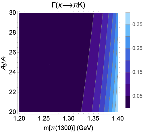
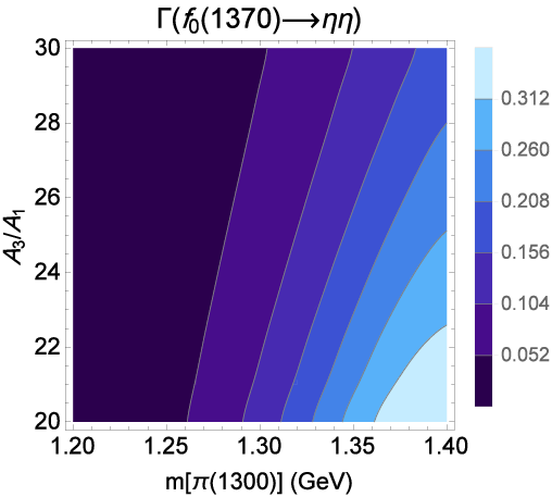
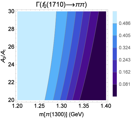
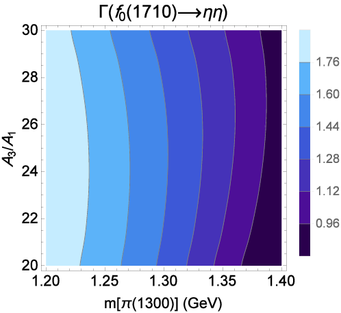
where AA, BB, C=1,2C=1,2 with 11 denoting nonet MM and 22 denoting nonet M′M^{\prime} and II, JJ, K=a,b,cK=a,\,b,\,c and dd represent the four bases in Eq. (15). L0L_{0}, RπR_{\pi}, LaL_{a}, R0R_{0}, LκL_{\kappa}, and RKR_{K} are the rotation matrices defined in Eqs. (13) and (14). The nonvanishing bare three-point coupling constants are given in Appendix A. The contour plots of all the hadronic two-body decay widths below 2 GeV are presented in Figs. 1-8. In the following we will explain each figure separately:
Refer to caption
Refer to caption
Refer to caption
Refer to caption
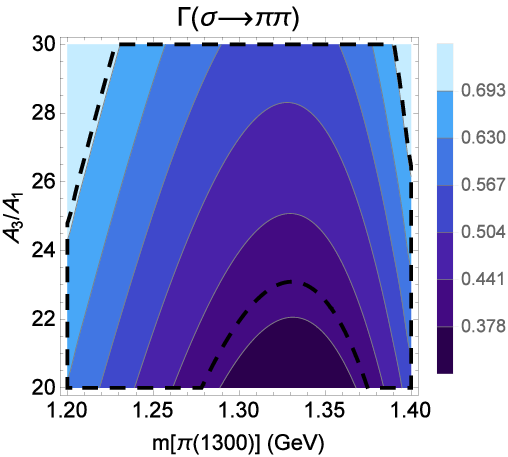
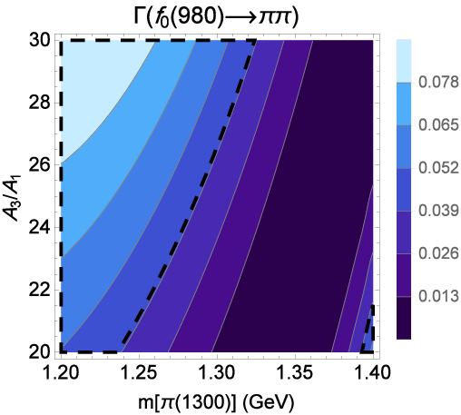
Figure 1: Contour plots of the prediction of the model for Γ[σ→ππ]\Gamma[\sigma\rightarrow\pi\pi] (top left), Γ[f0(980)→ππ]\Gamma[f_{0}(980)\rightarrow\pi\pi] (top right), Γ[κ→πK]\Gamma[\kappa\rightarrow\pi K] (bottom left) and Γ[a0(980)→πη]\Gamma[a_{0}(980)\rightarrow\pi\eta] (bottom right) over the m⁡[π⁡(1300)]m[\pi(1300)]-A3/A1A_{3}/A_{1} plane. The parameter spaces inside the dashed curves indicate regions for which decay widths are in the experimental range.

Figure 1:

In this figure we review the results for σ→π​π\sigma\rightarrow\pi\pi, f0​(980)→π​πf_{0}(980)\rightarrow\pi\pi, a0​(980)→π​ηa_{0}(980)\rightarrow\pi\eta and κ→π​K\kappa\rightarrow\pi K decay widths which are given in Ref. [41]. Contour plot for σ→π​π\sigma\rightarrow\pi\pi decay width shows that for a large part of the parameter space, the prediction of the model for this decay overlaps with the experimental data (The region inside the dashed curves show the experimental range for each decay). Also for f0​(980)→π​πf_{0}(980)\rightarrow\pi\pi and a0​(980)→π​ηa_{0}(980)\rightarrow\pi\eta decay widths, there exist regions of parameter space which agree with the experimental ranges. No region coincides with the experimental range for κ→π​K\kappa\rightarrow\pi K decay width, but for m⁡[π⁡(1300)]m[\pi(1300)] near 1.41.4 GeV, decay width reaches 400400 MeV which at least has a right order of magnitude compared to PDG data. The interesting point is that due to final state interactions in π​K\pi K scattering, total decay width for κ\kappa gets larger (It is shown in Ref. [39] and will be discussed in the next section).

Refer to caption
Refer to caption
Figure 2: Contour plots of the prediction of the model for Γ[a0(980)→KK¯]\Gamma[a_{0}(980)\rightarrow K\bar{K}] (left) and Γ[f0(980)→KK¯]\Gamma[f_{0}(980)\rightarrow K\bar{K}] (right) over the m⁡[π⁡(1300)]m[\pi(1300)]-A3/A1A_{3}/A_{1} plane. The white region belongs to zero value of decay width. As expected, decay widths are small for the main part of the parameter space.

Figure 2:

Since π​π\pi\pi and π​η\pi\eta decay modes are dominant channels for decays of f0​(980)f_{0}(980) and a0​(980)a_{0}(980), respectively, K​K¯K\bar{K} decay channel for these two particles should have narrow decay width. Fig. 2 shows that the model prediction for these channels fulfill our expectation: decay widths are small for some regions of the parameter space. Averaging over the entire parameter space, we have

Γ[a0(980)→KK¯]\displaystyle\Gamma[a_{0}(980)\rightarrow K\bar{K}] =\displaystyle= 21±27,\displaystyle 21\pm 27,
Γ[f0(980)→KK¯]\displaystyle\Gamma[f_{0}(980)\rightarrow K\bar{K}] =\displaystyle= 21±31,\displaystyle 21\pm 31, (26)

where the uncertainty is the standard deviation of the predicted data. These values are in agreement with the results of Refs. [45] and [46]. The prediction of the model over the m⁡[π⁡(1300)]−A3/A1m[\pi(1300)]-A_{3}/A_{1} plane for Γ[a0(980)→KK¯]/Γ[a0(980)→πη]\Gamma[a_{0}(980)\rightarrow K\bar{K}]/\Gamma[a_{0}(980)\rightarrow\pi\eta] is

Γ[a0(980)→KK¯]Γ[a0(980)→πη]=0.44±0.41.\frac{\Gamma[a_{0}(980)\rightarrow K\bar{K}]}{\Gamma[a_{0}(980)\rightarrow\pi\eta]}=0.44\pm 0.41. (27)

The mean value is about 2.52.5 times larger than the experimental value (Table 1) but the uncertainty covers the observed range.

Figure 3:

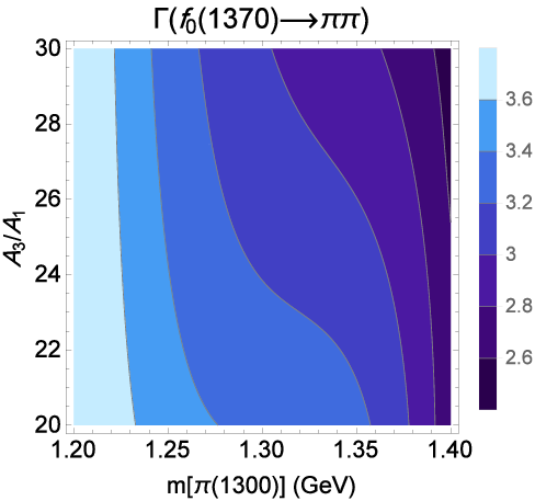
Now let us study hadronic decay widths above 1 GeV. It is shown in Ref. [20] that the GLSM prediction for the third f-meson mass is 1504±61504\pm 6, but due to unitarity corrections in π​π\pi\pi scattering [38], its mass reduces to 1149±431149\pm 43 which is close to f0​(1370)f_{0}(1370) mass. Furthermore, we know that broad states receive more contributions (in mass and width) from the unitarity corrections compared to the narrow ones. Therefore we identify the third f-meson predicted by our model with the broad state f0​(1370)f_{0}(1370) and not the narrow state f0​(1500)f_{0}(1500). This is consistent with the result of Ref. [47] in which it was shown that f0​(1500)f_{0}(1500) is the scalar glueball state. Moreover, f0​(1370)f_{0}(1370) was shown to be predominantly a quark-antiquark state (particularly s​s¯s\bar{s}) with small remnant of four quark and glue components [34]. Although there is no experimental data for decay widths of different modes of this broad resonance, Fig. 3 shows that for all the decay modes except π​π\pi\pi, the predicted decay widths are reasonable compared to the full width but Γ[f0(1370)→ππ]\Gamma[f_{0}(1370)\rightarrow\pi\pi] is extremely large and far from experiment. The predicted averaged value for Γ[f0(1370)→KK¯]\Gamma[f_{0}(1370)\rightarrow K\bar{K}] is 72±7672\pm 76 MeV in agreement with Ref. [48].

Figure 4:

For f0​(1710)f_{0}(1710) which decays predominantly into kaons, K​K¯K\bar{K} and η​η\eta\eta channels have large and unreasonable widths but their ratio is

Γ[f0(1710)→ηη]Γ[f0(1710)→KK¯]=0.42±0.04,\frac{\Gamma[f_{0}(1710)\rightarrow\eta\eta]}{\Gamma[f_{0}(1710)\rightarrow K\bar{K}]}=0.42\pm 0.04, (28)

which overlaps with the experimental range (Table 1). For π​π\pi\pi channel, decay width has the right order of magnitude compared to the full width for large values of m⁡[π⁡(1300)]m[\pi(1300)] and

Γ[f0(1710)→ππ]Γ[f0(1710)→KK¯]=0.10±0.05,\frac{\Gamma[f_{0}(1710)\rightarrow\pi\pi]}{\Gamma[f_{0}(1710)\rightarrow K\bar{K}]}=0.10\pm 0.05, (29)

which is not in the range of PDG data but consistent with the results of Ref. [49]:

Γ[f0(1710)→ππ]Γ[f0(1710)→KK¯]<0.11.\frac{\Gamma[f_{0}(1710)\rightarrow\pi\pi]}{\Gamma[f_{0}(1710)\rightarrow K\bar{K}]}<0.11.

Moreover the recent results of Refs. [50] and [51] have suggested that the f0​(1710)f_{0}(1710) is predominantly the glueball state and due to the fact that the glueball effects are not included in GLSM, we do not expect to get good results for decay widths of this state.
Refer to caption
Refer to caption
Refer to caption
Refer to caption
Figure 3: Contour plots of the prediction of the model for Γ[f0(1370)→ππ,KK¯,ηη,π(1300)π]\Gamma[f_{0}(1370)\rightarrow\pi\pi,\,K\bar{K},\,\eta\eta,\,\pi(1300)\pi] over the m⁡[π⁡(1300)]m[\pi(1300)]-A3/A1A_{3}/A_{1} plane. For all decay modes except π​π\pi\pi, predicted decay widths are reasonable compared to the full width.
Refer to caption
Refer to caption
Refer to caption
Figure 4: Contour plots of the prediction of the model for Γ[f0(1710)→ππ,KK¯,ηη]\Gamma[f_{0}(1710)\rightarrow\pi\pi,\,K\bar{K},\,\eta\eta] decay widths over the m⁡[π⁡(1300)]m[\pi(1300)]-A3/A1A_{3}/A_{1} plane. K​K¯K\bar{K} and η​η\eta\eta channels have large and unreasonable widths, but for π​π\pi\pi channel, decay width has the right order of magnitude for large values of m⁡[π⁡(1300)]m[\pi(1300)] compared to the full width.
Refer to caption
Figure 5: Contour plot of the prediction of the model for K0∗→π​KK_{0}^{*}\rightarrow\pi K decay width over the m⁡[π⁡(1300)]m[\pi(1300)]-A3/A1A_{3}/A_{1} plane. Decay width is too large but receives unitarity corrections due to the π​K\pi K final state interaction.
Refer to caption
Refer to caption
Refer to caption
Figure 6: Contour plot of the prediction of the model for Γ[a0(1450)→πη,KK¯,πη′]\Gamma[a_{0}(1450)\rightarrow\pi\eta,\,K\bar{K},\,\pi\eta^{\prime}] decay widths over the m⁡[π⁡(1300)]m[\pi(1300)]-A3/A1A_{3}/A_{1} plane. Γ[a0(1450)→πη′]\Gamma[a_{0}(1450)\rightarrow\pi\eta^{\prime}] is comparable with the experimental full width and the other two decay widths are too large but their ratio is in the experimental range.

Figure 5:

�Γ[K0∗(1430)→πK]ÃÂÂ\textasciimacron ¿ÂÂÂ\textonehalf\Gamma[K_{0}^{*}(1430)\rightarrow\pi K] is too large, but according to final state interactions of π​K\pi K which are estimated by the K-matrix unitarization method, decay width decreases [39], but this time becomes too small compared to the experiment (Table 4) and this convinces us that the current Lagrangian of the model, cannot describe energy region above 1 GeV for some processes and therefore is not complete.


Figure 6:

Among different hadronic channels for a0​(1450)a_{0}(1450) decay, only Γ[a0(1450)→πη′]\Gamma[a_{0}(1450)\rightarrow\pi\eta^{\prime}] is comparable with the experimental full width and the other two, i.e., π​η\pi\eta and K​K¯K\bar{K} widths, are too large but their ratio is in the experimental range

Γ[a0(1450)→KK¯]Γ[a0(1450)→πη]=0.96±0.10.\frac{\Gamma[a_{0}(1450)\rightarrow K\bar{K}]}{\Gamma[a_{0}(1450)\rightarrow\pi\eta]}=0.96\pm 0.10. (30)

It should be pointed that the final state interaction effects are also computed for π​η\pi\eta scattering [40] and fortunately the total width for a0​(1450)a_{0}(1450) which comes from the imaginary part of the K-matrix unitarized amplitude pole, is close to the experimental range (Table 4). This will be discussed in the next section.

Figure 7:

Decay widths of different modes of η⁡(1295)\eta(1295) are calculated within scenario 3​I3I which is the best scenario. Decay widths for both channels are consistent with the experimental data for small values of m⁡[π⁡(1300)]m[\pi(1300)] and their ratio is

Γ[η(1295)→a0(980)π]Γ[η(1295)→ση]=0.47±0.16,\frac{\Gamma[\eta(1295)\rightarrow a_{0}(980)\pi]}{\Gamma[\eta(1295)\rightarrow\sigma\eta]}=0.47\pm 0.16, (31)

which overlaps with the experimental range.

Figure 8:

To evaluate η⁡(1405)\eta(1405) and η⁡(1475)→a0​(980)​π\eta(1475)\rightarrow a_{0}(980)\pi decay widths, we used scenario 5​I5I and 6​I6I, respectively. Although η\eta masses predicted in these scenarios are less than expected values and these scenarios are clearly not favoured, but the resulting widths are comparable with the full experimental width (Fig. 8). Note that in our model, η⁡(1405)\eta(1405) can not decay into f0​(980)​ηf_{0}(980)\eta as its predicted mass is less than the threshold mass.

Refer to caption
Refer to caption
Figure 7: Contour plot of the prediction of the model for Γ[η(1295)→a0(980)π,ση]\Gamma[\eta(1295)\rightarrow a_{0}(980)\pi,\,\sigma\eta] decay widths over the m⁡[π⁡(1300)]m[\pi(1300)]-A3/A1A_{3}/A_{1} plane. Decay widths are consistent with the experimental data for smaller values of m⁡[π⁡(1300)]m[\pi(1300)].
Refer to caption
Refer to caption
Figure 8: Contour plots of the prediction of the model for Γ[η(1405)→a0(980)π]\Gamma[\eta(1405)\rightarrow a_{0}(980)\pi] and Γ[η(1475)→a0(980)π]\Gamma[\eta(1475)\rightarrow a_{0}(980)\pi] decay widths over the m⁡[π⁡(1300)]m[\pi(1300)]-A3/A1A_{3}/A_{1} plane. Decay widths are comparable with the full experimental widths.

In order to compare the predictions of the model with experimental data, the averaged values and the standard deviations over the m⁡[π⁡(1300)]−A3/A1m[\pi(1300)]-A_{3}/A_{1} plane for decay widths of lowest lying scalars and pseudoscalars are given in Table 2. Also the mean values for decay widths of next-to-lowest lying mesons are summarized in Table 3. Among these decays, nine of them overlap with the experimental range or at least have the right order of magnitude compared to the experimental full width. For the remaining decays, i.e., f0​(1370)→π​πf_{0}(1370)\rightarrow\pi\pi, f0​(1710)→K​K¯f_{0}(1710)\rightarrow K\bar{K}, f0​(1710)→η​ηf_{0}(1710)\rightarrow\eta\eta, K0∗​(1430)→π​KK_{0}^{*}(1430)\rightarrow\pi K, a0​(1450)→π​ηa_{0}(1450)\rightarrow\pi\eta and a0​(1450)→K​K¯a_{0}(1450)\rightarrow K\bar{K}, decay widths are too large.

One may argue that if we consider the effect of final state interactions in π​π\pi\pi, π​K\pi K and π​η\pi\eta scatterings within the GLSM framework, this may change the bare predictions of decay widths and masses of scalars to the acceptable ones. In the next section, we will review this effect.

Table 2: Predicted bare masses and decay widths of lowest lying mesons in the generalized linear sigma model.
 
 
GLSM
Width (MeV) Mass of decaying
particle (MeV)
 
σ→π​π\sigma\rightarrow\pi\pi 531±99531\pm 99 645±42645\pm 42
f0​(980)→π​πf_{0}(980)\rightarrow\pi\pi 35±2735\pm 27 1131±471131\pm 47
f0​(980)→K​K¯f_{0}(980)\rightarrow K\overline{K} 21±3121\pm 31 1131±471131\pm 47
κ→π​K\kappa\rightarrow\pi K 58±9058\pm 90 1105±281105\pm 28
a0​(980)→π​ηa_{0}(980)\rightarrow\pi\eta 57±4457\pm 44 980±20​a980\pm 20{\textsuperscript{a}}
a0​(980)→K​K¯a_{0}(980)\rightarrow K\overline{K} 21±2721\pm 27 980±20980\pm 20
 
 
  • a

    This shows experimental error bar; Other error bars are standard deviations of the mean value averaged over the m⁡[π⁡(1300)]−A3/A1m[\pi(1300)]-A_{3}/A_{1} plane.

Table 3: Predicted bare masses and decay widths of next-to-lowest lying mesons in GLSM.
 
 
decay modes GLSM     decay modes GLSM
width (MeV) mass of decaying     width (MeV) mass of decaying
particle(MeV)     particle(MeV)
 
f0​(1370)→π​πf_{0}(1370)\rightarrow\pi\pi 3216±3133216\pm 313 1504±61504\pm 6     a0​(1450)→π​ηa_{0}(1450)\rightarrow\pi\eta 1729±2781729\pm 278 1474±19​a1474\pm 19{\textsuperscript{a}}
f0​(1370)→K​K¯f_{0}(1370)\rightarrow K\overline{K} 72±7672\pm 76 1504±61504\pm 6     a0​(1450)→π​η′a_{0}(1450)\rightarrow\pi\eta^{\prime} 106±57106\pm 57 1474±191474\pm 19
f0​(1370)→η​ηf_{0}(1370)\rightarrow\eta\eta 107±98107\pm 98 1504±61504\pm 6     a0​(1450)→K​K¯a_{0}(1450)\rightarrow K\overline{K} 1660±2781660\pm 278 1474±191474\pm 19
f0​(1370)→π⁡(1300)​πf_{0}(1370)\rightarrow\pi(1300)\pi 59±5259\pm 52 1504±61504\pm 6     η⁡(1295)→a0​(980)​π\eta(1295)\rightarrow a_{0}(980)\pi b 62±3062\pm 30 1271±611271\pm 61
f0​(1710)→π​πf_{0}(1710)\rightarrow\pi\pi 339±204339\pm 204 1684±401684\pm 40     η⁡(1295)→σ​η\eta(1295)\rightarrow\sigma\etab 103±72103\pm 72 1271±611271\pm 61
f0​(1710)→K​K¯f_{0}(1710)\rightarrow K\overline{K} 3306±5233306\pm 523 1684±401684\pm 40     η⁡(1405)→a0​(980)​π\eta(1405)\rightarrow a_{0}(980)\pic 65±3565\pm 35 1274±591274\pm 59
f0​(1710)→η​ηf_{0}(1710)\rightarrow\eta\eta 1406±3371406\pm 337 1684±401684\pm 40     η⁡(1475)→a0​(980)​π\eta(1475)\rightarrow a_{0}(980)\pi d 69±3969\pm 39 1278±591278\pm 59
K0∗​(1430)→π​KK_{0}^{*}(1430)\rightarrow\pi K 4674±5624674\pm 562 1555±361555\pm 36    
 
 
  • a

    This shows experimental error bar; Other error bars are standard deviations of the mean value averaged over the m⁡[π⁡(1300)]−A3/A1m[\pi(1300)]-A_{3}/A_{1} plane.

  • b

    Scenario 3​I3I

  • c

    Scenario 5​I5I

  • d

    Scenario 6​I6I

4 Unitarity Corrections

In order to consider final state interactions in π​π\pi\pi, π​K\pi K and π​η\pi\eta scatterings, we use K-matrix unitarization method [38, 39, 40] through which the partial wave bare amplitude TlI​BT^{I\,B}_{l} transforms to unitarized amplitude TlIT^{I}_{l} using the following equation

TlI=TlI​B1−i​TlI​B,T^{I}_{l}=\frac{T^{I\,B}_{l}}{1-iT^{I\,B}_{l}}, (32)

where II and ll denote to the partial wave isospin and angular momentum. The poles of the K-matrix unitarized amplitude are used to calculate the physical masses and full decay widths of the intermediate scalar mesons. Here we review the π​π\pi\pi scattering [38] and the π​K\pi K and π​η\pi\eta scatterings are explored in Refs. [39, 40].

The K-matrix unitarized π​π\pi\pi scattering amplitude for the I=J=0I=J=0 channel is given by

T00=T00B1−i​T00B,T_{0}^{0}={{T_{0}^{0}}^{B}\over{1-i\,{T_{0}^{0}}^{B}}}, (33)

where T00B{T_{0}^{0}}^{B} is the “bare” scattering amplitude calculated from the Lagrangian in Eq. (4)

T00B=Tα+∑iTβimfi2−s,{T_{0}^{0}}^{B}=T_{\alpha}+\sum_{i}{{T_{\beta}^{i}}\over{m_{f_{i}}^{2}-s}}, (34)

with

Tα\displaystyle T_{\alpha} =\displaystyle= 164​π​1−4​mπ2s​[−5​γπ​π(4)+2pπ2​∑iγfi​π​π2​ln​(1+4​pπ2mfi2)],\displaystyle{1\over 64\pi}\sqrt{1-{4m_{\pi}^{2}\over s}}\,\left[-5\,\gamma^{(4)}_{\pi\pi}+{2\over{p_{\pi}^{2}}}\,\sum_{i}\gamma_{f_{i}\pi\pi}^{2}\,{\rm ln}\left(1+{{4p_{\pi}^{2}}\over m_{f_{i}}^{2}}\right)\right],
Tβi\displaystyle T_{\beta}^{i} =\displaystyle= 316​π​1−4​mπ2s​γfi​π​π2,\displaystyle{3\over 16\pi}\sqrt{1-{4m_{\pi}^{2}\over s}}\,\gamma_{f_{i}\pi\pi}^{2}, (35)

where pπ=s−4​mπ2/2p_{\pi}=\sqrt{s-4m_{\pi}^{2}}/2. The scalar-pseudoscalar-pseudoscalar couplings γfi​π​π\gamma_{f_{i}\pi\pi} are defined in Sec. 3, and γπ​π(4)\gamma^{(4)}_{\pi\pi} is the pion four-point coupling constant

g=⟨∂4V∂π+​∂π−​∂π+​∂π−⟩=∑A,B,C,D⟨∂4V∂(ϕ12)A​∂(ϕ21)B​∂(ϕ12)C​∂(ϕ21)D⟩​(Rπ)A​1​(Rπ)B​1​(Rπ)C​1​(Rπ)D​1,g=\left\langle{{\partial^{4}V}\over{\partial\pi^{+}\,\partial\pi^{-}\,\partial\pi^{+}\,\partial\pi^{-}}}\right\rangle=\sum_{A,B,C,D}\left\langle{{\partial^{4}V}\over{\partial(\phi_{1}^{2})_{A}\,\partial(\phi_{2}^{1})_{B}\,\partial(\phi_{1}^{2})_{C}\,\partial(\phi_{2}^{1})_{D}}}\right\rangle\,(R_{\pi})_{A1}\,(R_{\pi})_{B1}\,(R_{\pi})_{C1}\,(R_{\pi})_{D1}, (36)

where the sum is over “bare” pions and A,B,⋯A,B,\cdots = 1, 2 with 1 denoting nonet MM and 2 denoting nonet M′M^{\prime} and RπR_{\pi} is the pion rotation matrix. The real part of the unitarized scattering amplitude, Eq. (33), is plotted in Fig 9. It is clear that the prediction of the model is in reasonable qualitative agreement with the experimental data up to about 1 GeV.

Refer to caption
Figure 9: Real part of the unitarized scattering amplitude of π​π\pi\pi scattering for three different choices of m⁡[π⁡(1300)]m[\pi(1300)] and A3/A1=30A_{3}/A_{1}=30.

The physical pole positions in the unitarized scattering amplitude are determined by solving for the complex roots of the denominator of the K-matrix unitarized amplitude Eq. (33)

1−i​T00​B=0.1-iT_{0}^{0B}=0. (37)

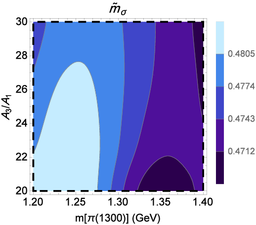
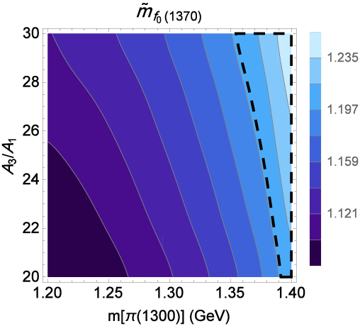
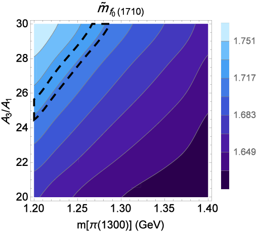
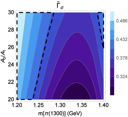
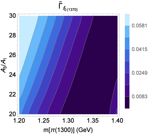
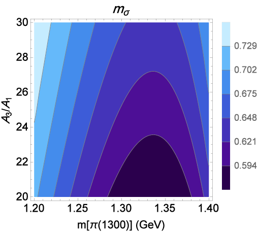
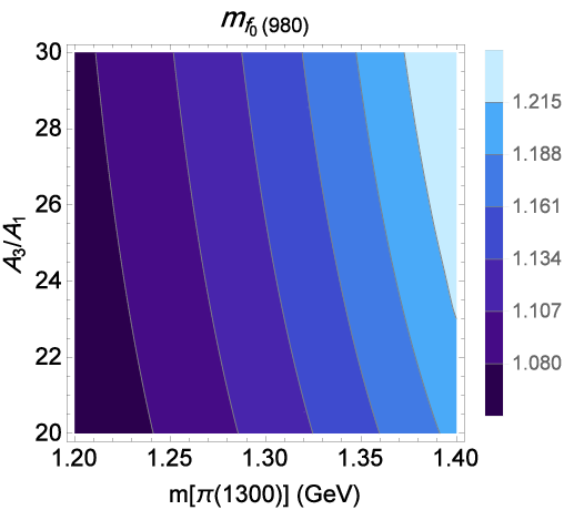
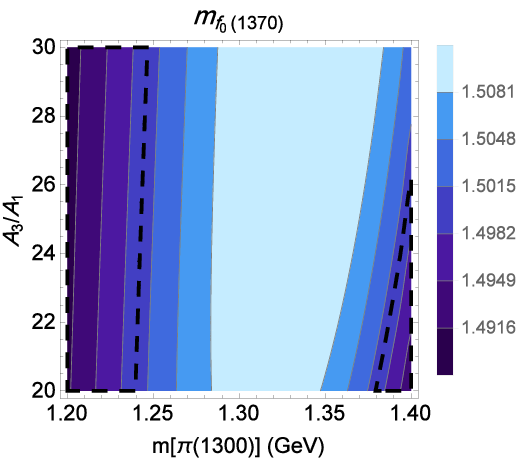
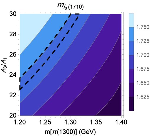
Each complex pole is equivalent to m~i2−i​m~​Γ~i{\tilde{m}}_{i}^{2}-i{\tilde{m}}{\tilde{\Gamma}}_{i}, where m~i{\tilde{m}}_{i} and Γ~i{\tilde{\Gamma}}_{i} are the physical mass and width of the ii-th pole. By solving Eq. (37) numerically, we will find four solutions for the pole positions, each corresponds to the physical mass and total width of fif_{i}’s. The masses and total widths of the π​π\pi\pi unitarized scattering amplitude are plotted in Figs. 10 and 11. Comparing the bare masses resulted from the Lagrangian (Fig. 12) with the physical masses obtained from the unitarized π​π\pi\pi scattering amplitude (Fig. 10), shows that the unitarization procedure reduces the bare masses of σ\sigma and f0​(980)f_{0}(980) which are located out of the experimental ranges to physical masses within the experimental bounds. It is clear from Figs. 1 and 11 that before and after unitarization there exists regions of parameter space for which decay widths of σ\sigma and f0​(980)f_{0}(980) cover the experimental ranges 11 1 As π​π\pi\pi channel is the dominant decay mode for σ\sigma and f0​(980)f_{0}(980) decays, total widths resulted from unitarization procedure are comparable with Γ[σ→ππ]\Gamma[\sigma\rightarrow\pi\pi] and Γ[f0(980)→ππ]\Gamma[f_{0}(980)\rightarrow\pi\pi].. Furthermore, for f0​(1370)f_{0}(1370) and f0​(1710)f_{0}(1710), the bare total widths (sum of the average values for different decay modes in Table 3), are too large compared to the experimental full width which proves the failure of the model for these decay widths. As we expected, the unitarization, makes the total widths smaller with respect to the previous values, but unfortunately too small compared to the experimental data (Fig. 11). The same unitarization procedure can be applied for π​K\pi K and π​η\pi\eta scatterings which leads to the unitarized masses and full widths for isodoublets (κ\kappa, K0∗K_{0}^{*}) and isotriplets (a0​(980)a_{0}(980),a0​(1450)a_{0}(1450)), respectively [39, 40].

Refer to caption
Refer to caption
Refer to caption
Refer to caption
Figure 10: Contour plots of the predictions of the GLSM for the physical masses of four f-mesons obtained from the poles of the K-matrix unitarized amplitude of π​π\pi\pi scattering over the m⁡[π⁡(1300)]−A3/A1m[\pi(1300)]-A_{3}/A_{1} plane. The parameter space inside the dashed curves indicate regions for which masses are in the experimental range.
Refer to caption
Refer to caption
Refer to caption
Refer to caption
Figure 11: Contour plots of the predictions of the GLSM for the physical widths of four f-mesons obtained from the poles of the K-matrix unitarized amplitude of π​π\pi\pi scattering over the m⁡[π⁡(1300)]−A3/A1m[\pi(1300)]-A_{3}/A_{1} plane. The parameter space inside the dashed curves indicate regions for which decay widths are in the experimental range.
Refer to caption
Refer to caption
Refer to caption
Refer to caption
Figure 12: Contour plots of the predictions of the GLSM for the bare masses of four f-mesons over the m⁡[π⁡(1300)]−A3/A1m[\pi(1300)]-A_{3}/A_{1} plane. The parameter space inside the dashed curves indicate regions for which decay widths are in the experimental range.

Finally, the mean values for physical masses and decay widths obtained from unitarization procedure corresponding to isosinglet, isodoublet and isotriplet scalar states are given in Table 4. It is clear that the averaged total widths of σ\sigma and a0​(980)a_{0}(980) with their uncertainty overlap with the experiment. For f0​(980)f_{0}(980), although the mean value of Γ~f0​(980)\tilde{\Gamma}_{f_{0}(980)} is not in agreement with the experimental data, it varies from 7575 to 335335 MeV which indeed for some regions of parameter space, total width overlaps with PDG data. Γ~κ\tilde{\Gamma}_{\kappa} does not agree with the experiment but is close to it. Thus, the poles in the unitarized scattering amplitude which represent physical states leads to the acceptable widths and masses for states below 1 GeV, while for the physical states above 1 GeV, the obtained total widths are too small compared to the expected values except for a0​(1450)a_{0}(1450).

Table 4: Predicted physical masses and decay widths of lowest lying and next-to-lowest lying mesons in GLSM obtained from unitarized amplitudes [38, 39, 40].
 
 
lowest lying     next-to-lowest lying
Width (MeV) Mass(MeV)     Width (MeV) Mass(MeV)
 
σ\sigma 385±61385\pm 61 476±4476\pm 4     f0​(1370)f_{0}(1370) 22±2122\pm 21 1149±431149\pm 43
f0​(980)f_{0}(980) 207±65207\pm 65 1053±441053\pm 44     f0​(1710)f_{0}(1710) 2±12\pm 1 1672±371672\pm 37
κ\kappa 689±27689\pm 27 722±28722\pm 28     K0∗​(1430)K_{0}^{*}(1430) 5±65\pm 6 1114±501114\pm 50
a0​(980)a_{0}(980) 60±5260\pm 52 984±7984\pm 7     a0​(1450)a_{0}(1450) 502±88502\pm 88 1085±431085\pm 43


5 Summary and conclusions

Table 5: Predicted bare masses and decay widths of lowest lying mesons in the non-renormalizable SU(3) single nonet linear sigma model (first column), the generalized linear sigma model (second column) and the decoupling limit of GLSM (third column).
 
 
SNLSM GLSM GLSM in decoupling limit
Width (MeV) Mass of decaying Width (MeV) Mass of decaying Width (MeV) Mass of decaying
particle (MeV) particle (MeV) particle (MeV)
 
σ→π​π\sigma\rightarrow\pi\pi 830830 847847 531±99531\pm 99 645±42645\pm 42 3077​a3077{\textsuperscript{a}} 960​a960{\textsuperscript{a}}
f0​(980)→π​πf_{0}(980)\rightarrow\pi\pi 41094109 13001300 35±2735\pm 27 1131±471131\pm 47 ...b...{\textsuperscript{b}} 1975±1171975\pm 117
f0​(980)→K​K¯f_{0}(980)\rightarrow K\overline{K} 15251525 13001300 21±3121\pm 31 1131±471131\pm 47 2424±462424\pm 46 1975±1171975\pm 117
κ→π​K\kappa\rightarrow\pi K 23502350 13001300 58±9058\pm 90 1105±281105\pm 28 1844±301844\pm 30 1202±221202\pm 22
a0​(980)→π​ηa_{0}(980)\rightarrow\pi\eta 381381 11001100 57±4457\pm 44 980±20​c980\pm 20{\textsuperscript{c}} 347±16347\pm 16 980±20980\pm 20
a0​(980)→K​K¯a_{0}(980)\rightarrow K\overline{K} 221221 11001100 21±2721\pm 27 980±20980\pm 20 161±100161\pm 100 980±20980\pm 20
 
 
  • a

    These values are independent of A3/A1A_{3}/A_{1} and therefore have no standard deviations.

  • b

    In the decoupling limit f0​(980)f_{0}(980) contains strange quarks and thus cannot couple with π\pi, i.e., γf2​π​π=0\gamma_{f_{2}\pi\pi}=0.

  • c

    This shows experimental error bar; Other error bars are standard deviations of the mean value averaged over the m⁡[π⁡(1300)]−A3/A1m[\pi(1300)]-A_{3}/A_{1} plane in case of GLSM or averaged over different values of A3/A1A_{3}/A_{1} in case of GLSM in decoupling limit.

In the present work, we have studied the effect of underlying mixing between q​q¯q\bar{q} and q​q​q¯​q¯qq\bar{q}\bar{q} components in hadronic two-body decays of scalar and pseudoscalar mesons below 2 GeV within the GLSM. To see whether the mixing effect could improve the prediction of SNLSM for lowest lying scalars [44], a comparison is made between predicted decay widths evaluated in these models ( first two columns of Table 5 ). At first sight, it is clear that the predictions have greatly improved in GLSM. So this model not only determines quark structure of mesons but also can improve the predictions for decays and certainly scatterings of mesons [38, 39, 40].
We should note that the masses of σ\sigma, f0​(980)f_{0}(980) and their mixing angle θs\theta_{s}, the mass of a0​(980)a_{0}(980) in the isotopic spin invariant limit and therefore the related vertices such as γσ​π​π\gamma_{\sigma\pi\pi} and γf2​π​π\gamma_{f_{2}\pi\pi} are not predicted in SNLSM directly: The isoscalar masses (m⁡[σ]m[\sigma], m​[f0​(980)]m[f_{0}(980)]) and consequently widths in Table 5 comes from the best fit for the real part of the I=J=0I=J=0, π​π\pi\pi scattering amplitude. Also the isovector mass (m[a0(980)m[a_{0}(980)]) can not be predicted from the SNLSM and an arbitrary value should be chosen for it; But in GLSM, all the masses and widths are direct predictions of the model and this is another advantage of GLSM versus SNLSM.

We have also evaluated all the lowest lying decay widths in the decoupling limit 22 2 Further discussion on decoupling limit is given in B (d2,e3a→0d_{2},\,e_{3}^{a}\rightarrow 0 and γ1→1\gamma_{1}\rightarrow 1) given in the third column of Table 5 in order to show that mixing provides much better description of decay widths. It is seen that by decoupling the four-quark fields, the results go far from the experimental data.

As a result, it has become clear that the GLSM Lagrangian at the present order of N=8N=8 with 88 experimental inputs and without any further tuning is successful in predicting decay widths of lowest lying mesons, while the predictions of SNLSM model are far from the expected values. Therefore, inclusion of the underlying mixings considerably improves the results for the decay widths.

We should notice that GLSM can not give acceptable widths for some states above 1 GeV. It would be worthwhile to study the effects of adding terms with higher than eight quark and antiquark lines and also considering the effects of scalar and pseudoscalar glueballs in potential. Our initial estimate shows that adding scalar and pseudoscalar glueballs has more considerable effects than adding terms with higher order of NN.

Acknowledgments

Authors would like to express sincere thanks towards A. H. Fariborz without whom it was impossible to accomplish this research.

Appendix A Three-point bare couplings

⟨∂3V∂(S12)1​∂(ϕ21)1​∂ηa⟩\displaystyle\left\langle\frac{\partial^{3}V}{\partial(S_{1}^{2})_{1}\partial(\phi_{2}^{1})_{1}\partial\eta_{a}}\right\rangle =\displaystyle= 4​2​(2​c4a​α15​β1+c4a​α14​α3​β3+2​c3​α3​β3​γ12+2​c3​α1​β1​γ1​(1+γ1))α13​(2​α1​β1+α3​β3),\displaystyle\frac{4\sqrt{2}\Big(2c_{4}^{a}\alpha_{1}^{5}\beta_{1}+c_{4}^{a}\alpha_{1}^{4}\alpha_{3}\beta_{3}+2c_{3}\alpha_{3}\beta_{3}\gamma_{1}^{2}+2c_{3}\alpha_{1}\beta_{1}\gamma_{1}(1+\gamma_{1})\Big)}{\alpha_{1}^{3}(2\alpha_{1}\beta_{1}+\alpha_{3}\beta_{3})}, (38)
⟨∂3V∂(S12)1​∂(ϕ21)2​∂ηa⟩\displaystyle\left\langle\frac{\partial^{3}V}{\partial(S_{1}^{2})_{1}\partial(\phi_{2}^{1})_{2}\partial\eta_{a}}\right\rangle =\displaystyle= −8​2​c3​(−1+γ1)​(α3​β3​γ1+α1​β1​(1+γ1))α1(2α1β1+α3β3)2,\displaystyle-\frac{8\sqrt{2}c_{3}\left(-1+\gamma_{1}\right)\Big(\alpha_{3}\beta_{3}\gamma_{1}+\alpha_{1}\beta_{1}\left(1+\gamma_{1}\right)\Big)}{\alpha_{1}\left(2\alpha_{1}\beta_{1}+\alpha_{3}\beta_{3}\right){}^{2}}, (39)
⟨∂3V∂(S12)2​∂(ϕ21)1​∂ηa⟩\displaystyle\left\langle\frac{\partial^{3}V}{\partial(S_{1}^{2})_{2}\partial(\phi_{2}^{1})_{1}\partial\eta_{a}}\right\rangle =\displaystyle= 8​2​c3​(−1+γ1)​(α3​β3​γ1+α1​β1​(1+γ1))α1(2α1β1+α3β3)2,\displaystyle\frac{8\sqrt{2}c_{3}\left(-1+\gamma_{1}\right)\Big(\alpha_{3}\beta_{3}\gamma_{1}+\alpha_{1}\beta_{1}\left(1+\gamma_{1}\right)\Big)}{\alpha_{1}\left(2\alpha_{1}\beta_{1}+\alpha_{3}\beta_{3}\right){}^{2}}, (40)
⟨∂3V∂(S12)1​∂(ϕ21)1​∂ηb⟩\displaystyle\left\langle\frac{\partial^{3}V}{\partial(S_{1}^{2})_{1}\partial(\phi_{2}^{1})_{1}\partial\eta_{b}}\right\rangle =\displaystyle= 8​c3​γ1​(α3​β3+2​α1​β1​γ1)α12​α3​(2​α1​β1+α3​β3),\displaystyle\frac{8c_{3}\gamma_{1}\left(\alpha_{3}\beta_{3}+2\alpha_{1}\beta_{1}\gamma_{1}\right)}{\alpha_{1}^{2}\alpha_{3}\left(2\alpha_{1}\beta_{1}+\alpha_{3}\beta_{3}\right)}, (41)
⟨∂3V∂(S12)1​∂(ϕ21)2​∂ηb⟩\displaystyle\left\langle\frac{\partial^{3}V}{\partial(S_{1}^{2})_{1}\partial(\phi_{2}^{1})_{2}\partial\eta_{b}}\right\rangle =\displaystyle= 4​e3a−8​c3​(−1+γ1)​(α3​β3+2​α1​β1​γ1)α3(2α1β1+α3β3)2,\displaystyle 4e_{3}^{a}-\frac{8c_{3}\left(-1+\gamma_{1}\right)\left(\alpha_{3}\beta_{3}+2\alpha_{1}\beta_{1}\gamma_{1}\right)}{\alpha_{3}\left(2\alpha_{1}\beta_{1}+\alpha_{3}\beta_{3}\right){}^{2}}, (42)
⟨∂3V∂(S12)2​∂(ϕ21)1​∂ηb⟩\displaystyle\left\langle\frac{\partial^{3}V}{\partial(S_{1}^{2})_{2}\partial(\phi_{2}^{1})_{1}\partial\eta_{b}}\right\rangle =\displaystyle= 4​e3a+8​c3​(−1+γ1)​(α3​β3+2​α1​β1​γ1)α3(2α1β1+α3β3)2,\displaystyle 4e_{3}^{a}+\frac{8c_{3}\left(-1+\gamma_{1}\right)\left(\alpha_{3}\beta_{3}+2\alpha_{1}\beta_{1}\gamma_{1}\right)}{\alpha_{3}\left(2\alpha_{1}\beta_{1}+\alpha_{3}\beta_{3}\right){}^{2}}, (43)
⟨∂3V∂(S12)1​∂(ϕ21)1​∂ηc⟩\displaystyle\left\langle\frac{\partial^{3}V}{\partial(S_{1}^{2})_{1}\partial(\phi_{2}^{1})_{1}\partial\eta_{c}}\right\rangle =\displaystyle= 8​2​c3​(−1+γ1)​γ1α1​(2​α1​β1+α3​β3),\displaystyle\frac{8\sqrt{2}c_{3}\left(-1+\gamma_{1}\right)\gamma_{1}}{\alpha_{1}\left(2\alpha_{1}\beta_{1}+\alpha_{3}\beta_{3}\right)}, (44)
⟨∂3V∂(S12)1​∂(ϕ21)2​∂ηc⟩\displaystyle\left\langle\frac{\partial^{3}V}{\partial(S_{1}^{2})_{1}\partial(\phi_{2}^{1})_{2}\partial\eta_{c}}\right\rangle =\displaystyle= −82c3α1(−1+γ1)2(2α1β1+α3β3)2,\displaystyle-\frac{8\sqrt{2}c_{3}\alpha_{1}\left(-1+\gamma_{1}\right){}^{2}}{\left(2\alpha_{1}\beta_{1}+\alpha_{3}\beta_{3}\right){}^{2}}, (45)
⟨∂3V∂(S12)2​∂(ϕ21)1​∂ηc⟩\displaystyle\left\langle\frac{\partial^{3}V}{\partial(S_{1}^{2})_{2}\partial(\phi_{2}^{1})_{1}\partial\eta_{c}}\right\rangle =\displaystyle= 82c3α1(−1+γ1)2(2α1β1+α3β3)2,\displaystyle\frac{8\sqrt{2}c_{3}\alpha_{1}\left(-1+\gamma_{1}\right){}^{2}}{\left(2\alpha_{1}\beta_{1}+\alpha_{3}\beta_{3}\right){}^{2}}, (46)
⟨∂3V∂(S12)1​∂(ϕ21)1​∂ηd⟩\displaystyle\left\langle\frac{\partial^{3}V}{\partial(S_{1}^{2})_{1}\partial(\phi_{2}^{1})_{1}\partial\eta_{d}}\right\rangle =\displaystyle= 8​e3a​α13​β1+4​e3a​α12​α3​β3+8​c3​α3​(−1+γ1)​γ1α12​(2​α1​β1+α3​β3),\displaystyle\frac{8e_{3}^{a}\alpha_{1}^{3}\beta_{1}+4e_{3}^{a}\alpha_{1}^{2}\alpha_{3}\beta_{3}+8c_{3}\alpha_{3}\left(-1+\gamma_{1}\right)\gamma_{1}}{\alpha_{1}^{2}\left(2\alpha_{1}\beta_{1}+\alpha_{3}\beta_{3}\right)}, (47)
⟨∂3V∂(S12)1​∂(ϕ21)2​∂ηd⟩\displaystyle\left\langle\frac{\partial^{3}V}{\partial(S_{1}^{2})_{1}\partial(\phi_{2}^{1})_{2}\partial\eta_{d}}\right\rangle =\displaystyle= −8c3α3(−1+γ1)2(2α1β1+α3β3)2,\displaystyle-\frac{8c_{3}\alpha_{3}\left(-1+\gamma_{1}\right){}^{2}}{\left(2\alpha_{1}\beta_{1}+\alpha_{3}\beta_{3}\right){}^{2}}, (48)
⟨∂3V∂(S12)2​∂(ϕ21)1​∂ηd⟩\displaystyle\left\langle\frac{\partial^{3}V}{\partial(S_{1}^{2})_{2}\partial(\phi_{2}^{1})_{1}\partial\eta_{d}}\right\rangle =\displaystyle= 8c3α3(−1+γ1)2(2α1β1+α3β3)2,\displaystyle\frac{8c_{3}\alpha_{3}\left(-1+\gamma_{1}\right){}^{2}}{\left(2\alpha_{1}\beta_{1}+\alpha_{3}\beta_{3}\right){}^{2}}, (49)
⟨∂3V∂(S23)1​∂(ϕ12)1​∂(ϕ31)1⟩\displaystyle\left\langle\frac{\partial^{3}V}{\partial(S_{2}^{3})_{1}\partial(\phi_{1}^{2})_{1}\partial(\phi_{3}^{1})_{1}}\right\rangle =\displaystyle= 4​α3​c4a,\displaystyle 4\alpha_{3}c_{4}^{a}, (50)
⟨∂3V∂(S23)2​∂(ϕ12)1​∂(ϕ31)1⟩\displaystyle\left\langle\frac{\partial^{3}V}{\partial(S_{2}^{3})_{2}\partial(\phi_{1}^{2})_{1}\partial(\phi_{3}^{1})_{1}}\right\rangle =\displaystyle= ⟨∂3V∂(S23)1​∂(ϕ12)1​∂(ϕ31)2⟩=⟨∂3V∂(S23)1​∂(ϕ12)2​∂(ϕ31)1⟩=−4​e3a,\displaystyle\left\langle\frac{\partial^{3}V}{\partial(S_{2}^{3})_{1}\partial(\phi_{1}^{2})_{1}\partial(\phi_{3}^{1})_{2}}\right\rangle=\left\langle\frac{\partial^{3}V}{\partial(S_{2}^{3})_{1}\partial(\phi_{1}^{2})_{2}\partial(\phi_{3}^{1})_{1}}\right\rangle=-4e_{3}^{a}, (51)
⟨∂3V∂fa​∂(ϕ13)1​∂(ϕ31)1⟩\displaystyle\left\langle\frac{\partial^{3}V}{\partial f_{a}\partial(\phi_{1}^{3})_{1}\partial(\phi_{3}^{1})_{1}}\right\rangle =\displaystyle= 2​2​c4a​(2​α1−α3),\displaystyle 2\sqrt{2}c_{4}^{a}(2\alpha_{1}-\alpha_{3}), (52)
⟨∂3V∂fb​∂(ϕ13)1​∂(ϕ31)1⟩\displaystyle\left\langle\frac{\partial^{3}V}{\partial f_{b}\partial(\phi_{1}^{3})_{1}\partial(\phi_{3}^{1})_{1}}\right\rangle =\displaystyle= −4​c4a​(α1−2​α3),\displaystyle-4c_{4}^{a}(\alpha_{1}-2\alpha_{3}), (53)
⟨∂3V∂fc​∂(ϕ13)1​∂(ϕ31)1⟩\displaystyle\left\langle\frac{\partial^{3}V}{\partial f_{c}\partial(\phi_{1}^{3})_{1}\partial(\phi_{3}^{1})_{1}}\right\rangle =\displaystyle= ⟨∂3V∂fa​∂(ϕ13)1​∂(ϕ31)2⟩=⟨∂3V∂fa​∂(ϕ13)2​∂(ϕ31)1⟩=2​2​e3a,\displaystyle\left\langle\frac{\partial^{3}V}{\partial f_{a}\partial(\phi_{1}^{3})_{1}\partial(\phi_{3}^{1})_{2}}\right\rangle=\left\langle\frac{\partial^{3}V}{\partial f_{a}\partial(\phi_{1}^{3})_{2}\partial(\phi_{3}^{1})_{1}}\right\rangle=2\sqrt{2}e_{3}^{a}, (54)
⟨∂3V∂fa​∂(ϕ12)1​∂(ϕ21)1⟩\displaystyle\left\langle\frac{\partial^{3}V}{\partial f_{a}\partial(\phi_{1}^{2})_{1}\partial(\phi_{2}^{1})_{1}}\right\rangle =\displaystyle= 4​2​c4a​α1,\displaystyle 4\sqrt{2}c_{4}^{a}\alpha_{1}, (55)
⟨∂3V∂fb​∂(ϕ12)1​∂(ϕ21)2⟩\displaystyle\left\langle\frac{\partial^{3}V}{\partial f_{b}\partial(\phi_{1}^{2})_{1}\partial(\phi_{2}^{1})_{2}}\right\rangle =\displaystyle= ⟨∂3V∂fb​∂(ϕ12)2​∂(ϕ21)1⟩=⟨∂3V∂fd​∂(ϕ12)1​∂(ϕ21)1⟩=4​e3a,\displaystyle\left\langle\frac{\partial^{3}V}{\partial f_{b}\partial(\phi_{1}^{2})_{2}\partial(\phi_{2}^{1})_{1}}\right\rangle=\left\langle\frac{\partial^{3}V}{\partial f_{d}\partial(\phi_{1}^{2})_{1}\partial(\phi_{2}^{1})_{1}}\right\rangle=4e_{3}^{a}, (56)
⟨∂3V∂(S12)1​∂(ϕ23)1​∂(ϕ31)1⟩\displaystyle\left\langle\frac{\partial^{3}V}{\partial(S_{1}^{2})_{1}\partial(\phi_{2}^{3})_{1}\partial(\phi_{3}^{1})_{1}}\right\rangle =\displaystyle= 4​c4a​(2​α1−α3),\displaystyle 4c_{4}^{a}(2\alpha_{1}-\alpha_{3}), (57)
⟨∂3V∂(S12)1​∂(ϕ23)1​∂(ϕ31)2⟩\displaystyle\left\langle\frac{\partial^{3}V}{\partial(S_{1}^{2})_{1}\partial(\phi_{2}^{3})_{1}\partial(\phi_{3}^{1})_{2}}\right\rangle =\displaystyle= ⟨∂3V∂(S12)1​∂(ϕ23)2​∂(ϕ31)1⟩=⟨∂3V∂(S12)2​∂(ϕ23)1​∂(ϕ31)1⟩=−4​e3a.\displaystyle\left\langle\frac{\partial^{3}V}{\partial(S_{1}^{2})_{1}\partial(\phi_{2}^{3})_{2}\partial(\phi_{3}^{1})_{1}}\right\rangle=\left\langle\frac{\partial^{3}V}{\partial(S_{1}^{2})_{2}\partial(\phi_{2}^{3})_{1}\partial(\phi_{3}^{1})_{1}}\right\rangle=-4e_{3}^{a}. (58)

Appendix B Decoupling limit of GLSM

The four-quark fields are decoupled in the limit d2,e3a→0d_{2},e_{3}^{a}\rightarrow 0 and γ1→1\gamma_{1}\rightarrow 1. To find five unknown parameters in this limit (c2,c4a,A1,A3,α1,α3)(c_{2},c_{4}^{a},A_{1},A_{3},\alpha_{1},\alpha_{3}), we use mπm_{\pi}, mam_{a} and A3/A1A_{3}/A_{1} as experimental inputs

mπ2\displaystyle m_{\pi}^{2} =\displaystyle= −2​c2+4​c4a​α12,\displaystyle-2c_{2}+4c_{4}^{a}\alpha_{1}^{2},
ma2\displaystyle m_{a}^{2} =\displaystyle= −2​c2+12​c4a​α12,\displaystyle-2c_{2}+12c_{4}^{a}\alpha_{1}^{2},
A3A1\displaystyle\frac{A_{3}}{A_{1}} =\displaystyle= 20→30,\displaystyle 20\rightarrow 30,
Fπ\displaystyle F_{\pi} =\displaystyle= 2​α1,\displaystyle 2\alpha_{1}, (59)

besides two minimum equations

−2​A1+4​caa​α13−2​α1​c2\displaystyle-2A_{1}+4c_{a}^{a}\alpha_{1}^{3}-2\alpha_{1}c_{2} =\displaystyle= 0,\displaystyle 0,
−2​A3+4​caa​α33−2​α3​c2\displaystyle-2A_{3}+4c_{a}^{a}\alpha_{3}^{3}-2\alpha_{3}c_{2} =\displaystyle= 0.\displaystyle 0. (60)

The experimental input for the determination of the remaining parameter c3c_{3} is Tr⁡(Mη2){\rm Tr(M_{\eta}^{2})}

mη2+mη2′=−4​c2−16​c3α12+4​c4a​α12−8​c3α32+4​c4a​α32.m_{\eta}^{2}+m_{\eta}^{{}^{\prime}2}=-4c_{2}-\frac{16c_{3}}{\alpha_{1}^{2}}+4c_{4}^{a}\alpha_{1}^{2}-\frac{8c_{3}}{\alpha_{3}^{2}}+4c_{4}^{a}\alpha_{3}^{2}. (61)

In this limit, the physical vertices are

γσ​π​π\displaystyle\gamma_{\sigma\pi\pi} =\displaystyle= 4​c4a​α1,\displaystyle 4c_{4}^{a}\alpha_{1},
γf0​π​π\displaystyle\gamma_{f_{0}\pi\pi} =\displaystyle= 0,\displaystyle 0,
γf2​K​K\displaystyle\gamma_{f_{2}KK} =\displaystyle= −4​2​c4a​α1+8​2​c4a​α3,\displaystyle-4\sqrt{2}c_{4}^{a}\alpha_{1}+8\sqrt{2}c_{4}^{a}\alpha_{3},
γκ​π​K\displaystyle\gamma_{\kappa\pi K} =\displaystyle= 4​c4a​α3,\displaystyle 4c_{4}^{a}\alpha^{3},
γa0​π​η\displaystyle\gamma_{a_{0}\pi\eta} =\displaystyle= 8​2​c3​cos⁡(θp)α13+4​2​c4a​cos⁡(θp)​α1−8​c3​sin⁡(θp)α12​α3,\displaystyle\frac{8\sqrt{2}\,c_{3}\cos(\theta_{p})}{\alpha_{1}^{3}}+4\sqrt{2}\,c_{4}^{a}\cos(\theta_{p})\alpha_{1}-\frac{8\,c_{3}\sin(\theta_{p})}{\alpha_{1}^{2}\alpha_{3}},
γa0​K​K\displaystyle\gamma_{a_{0}KK} =\displaystyle= 8​c4a​α1−4​c4a​α3,\displaystyle 8c_{4}^{a}\alpha_{1}-4c_{4}^{a}\alpha_{3}, (62)

where θp\theta_{p} is the pseudoscalar mixing angle.

[ηη′]=[cos⁡θp−sin⁡θpsin⁡θpcos⁡θp]​[ηaηb].\left[\begin{array}[]{cc}\eta\\ \eta^{\prime}\end{array}\right]=\left[\begin{array}[]{cc}\cos\theta_{p}&-\sin\theta_{p}\\ \sin\theta_{p}&\cos\theta_{p}\end{array}\right]\left[\begin{array}[]{cc}\eta_{a}\\ \eta_{b}\end{array}\right]. (63)

References

  • [1] J. Gasser and H. Leutwyler, Annals Phys. 158, 142 (1984);
  • [2] J. Gasser and H. Leutwyler, Nucl. Phys. B 250, 465 (1985);
  • [3] H. Leutwyler, Annals of Physics, 235, 165 (1994);
  • [4] S. Weinberg, Physica A (Amesterdam) 96, 327 (1979);
  • [5] S. Weinberg, arXiv:0908.1964v3 [hep-th] (2009);
  • [6] S. Scherer, Adv. Nucl. Phys. 27, 277 (2003);
  • [7] G. Ecker, Prog. Part. Nucl. Phys. 35, 1 (1995).
  • [8] M. Gell-Mann and M. Levy, II Nuovo Cimento 16, 705 (1960);
  • [9] D. Friedan, Phys. Rev. Lett. 45, 1057 (1980);
  • [10] S. Coleman, J. Wess, B. Zumino, Phys. Rev. 177, 2239 (1969);
  • [11] J. Honerkamp and K. Meetz, Phys. Rev. D 3, 1996 (1971);
  • [12] I. S. Gerstein, R. Jackiw, B. W. Lee and S. Weinberg , Phys. Rev. D 3, 2486 (1971);
  • [13] L. D. Faddeev, A. A. Slavnov, Theor. Math. Phys. 8, 843 (1971).
  • [14] D. Parganlija, F. Giacosa and D. H. Rischke, Phys. Rev. D 82, 054024 (2010);
  • [15] S. Janowski, D. Parganlija, F. Giacosa and D. H. Rischke, Phys. Rev. D 84, 054007 (2011);
  • [16] A. Habersetzer, arXiv:1301.4035 [hep-ph].
  • [17] A. H. Fariborz, R. Jora and J. Schechter, Phys. Rev. D 72, 034001 (2005).
  • [18] A. H. Fariborz, R. Jora and J. Schechter, Phys. Rev. D 76, 114001 (2007).
  • [19] A. H. Fariborz, R. Jora and J. Schechter, Phys. Rev. D 77, 094004 (2008).
  • [20] A. H. Fariborz, R. Jora and J. Schechter, Phys. Rev. D 79, 074014 (2009).
  • [21] R. L. Jaffe, Phys. Rev. D 15, 267 (1977); R. L. Jaffe, Phys. Rev. D 15, 281 (1977);
  • [22] M. G. Alford and R. L. Jaffe, Nucl. Phys. B 578, 367 (2000).
  • [23] R. L. Jaffe and F. Wilczek, Phys. Rev. Lett. 91, 232003 (2003).
  • [24] L. Maiani, F. Piccinini, A. D. Polosa and V. Riquer, Phys. Rev. Lett. 93, 212002 (2004).
  • [25] J. R. Pelaez, Phys. Rev. Lett. 92, 102001 (2004).
  • [26] J. R. Pelaez and G. Rios, Phys. Rev. Lett. 97, 242002 (2006).
  • [27] M. Napsuciale and S. Rodriguez, Phys. Rev. D 70, 094043 (2004);
  • [28] T. Teshima, I. Kitamura, and N. Morisita, J. Phys. G 28, 1391 (2002); 30, 663 (2004).
  • [29] F. Close and N. Tornqvist, J. Phys. G 28, R249(2002).
  • [30] A. H. Fariborz, Int. J. Mod. Phys. A 19, 2095 (2004).
  • [31] G. ’t Hooft, G. Isidori, L. Maiani, A.D. Polosa and V. Riquer, Phys. Lett. B 662, 424 (2008).
  • [32] A. H. Fariborz, Phys. Rev. D 74, 054030 (2006).
  • [33] A. H. Fariborz, R. Jora and J. Schechter, Phys. Rev. D 76, 014011 (2007).
  • [34] A. H. Fariborz, A. Azizi, and A. Asrar, Phys. Rev. D 91, 073013 (2015).
  • [35] J. Vijande, A. Valcarce, F. Fernandez and B. Silvestre-Brac, Phys. Rev. D 72, 034025 (2005).
  • [36] M. Napsuciale and S. Rodriguez, Phys. Lett. B 603, 195 (2004).
  • [37] D. Black, A. H. Fariborz and J. Schechter, Phys. Rev. D 61, 074001 (2000).
  • [38] A. H. Fariborz, R. Jora, J. Schechter, and M. N. Shahid, Phys. Rev. D 84, 113004 (2011).
  • [39] A. H. Fariborz, E. Pourjafarabadi, J. Schechter, S. Zarepour, and S. M. Zebarjad (unpublished).
  • [40] A. H. Fariborz, E. Pourjafarabadi, J. Schechter, S. Zarepour, and S. M. Zebarjad (unpublished).
  • [41] A. H. Fariborz, J. Schechter, S. Zarepour, and S. M. Zebarjad, Phys. Rev. D 90, 033009 (2014).
  • [42] K.A. Olive et al. (Particle Data Group), Chin. Phys. C 38, 090001 (2014).
  • [43] S. Aoki, Y. Aoki, C. Bernard, T. Blum, G. Colangelo, et al., Eur. Phys. J. C 74, 2890 (2014), arXiv:1310.8555 [hep-lat].
  • [44] D. Black, A. H. Fariborz, S. Moussa, S. Nasri, and J. Schechter, Phys. Rev. D 64, 014031 (2001).
  • [45] V. V. Anisovich, V. A. Nikonov and A. V. Sarantsev, Phys. Atom. Nucl. 65, 1545 (2002), arXiv:0102338 [hep-ph].
  • [46] L. Maiani, A. Polosa, F. Piccinini and V. Riquer, Phys. Rev. Lett. 93, 212002 (2004).
  • [47] C. Amsler and F. E. Close, Phys. Rev. D 53, 295 (1996).
  • [48] S. Janowski and F. Giacosa, J. Phys.: Conf. Ser. 503, 012029 (2014).
  • [49] M. Ablikim et al. [BES Collaboration], Phys. Lett. B 603, 138 (2004).
  • [50] D. Parganlija, P. Kovacs, G. Wolf, F. Giacosa and D. H. Rischke, Phys. Rev. D 87, 014011 (2013).
  • [51] S. Janowski, F. Giacosa and D. H. Rischke, Phys. Rev. D 90, 114005 (2014).