Hybrid Algorithm for Multi-Objective Optimization by Greedy Hypervolume Maximization
Abstract
This paper introduces a high-performance hybrid algorithm, called Hybrid Hypervolume Maximization Algorithm (H2MA), for multi-objective optimization that alternates between exploring the decision space and exploiting the already obtained non-dominated solutions. The proposal is centered on maximizing the hypervolume indicator, thus converting the multi-objective problem into a single-objective one. The exploitation employs gradient-based methods, but considering a single candidate efficient solution at a time, to overcome limitations associated with population-based approaches and also to allow an easy control of the number of solutions provided. There is an interchange between two steps. The first step is a deterministic local exploration, endowed with an automatic procedure to detect stagnation. When stagnation is detected, the search is switched to a second step characterized by a stochastic global exploration using an evolutionary algorithm. Using five ZDT benchmarks with 30 variables, the performance of the new algorithm is compared to state-of-the-art algorithms for multi-objective optimization, more specifically NSGA-II, SPEA2, and SMS-EMOA. The solutions found by the H2MA guide to higher hypervolume and smaller distance to the true Pareto frontier with significantly less function evaluations, even when the gradient is estimated numerically. Furthermore, although only continuous decision spaces have been considered here, discrete decision spaces could also have been treated, replacing gradient-based search by hill-climbing. Finally, a thorough explanation is provided to support the expressive gain in performance that was achieved.
Index Terms:
Exploration-exploitation algorithm; Gradient-based optimization; Hypervolume maximization; Multi-objective optimization.I Introduction
Multi-objective optimization (MOO) is a generalization of the standard single-objective optimization to problems where multiple criteria are defined and they conflict with each other [1]. In this case, there can be multiple optimal solutions with different trade-offs between the objectives. Since the optimal set can be continuous, an MOO problem is given by finding samples from the optimal set, called Pareto set. However, we also wish that the projection of the obtained samples of the Pareto set into the objective space be well-distributed along the Pareto frontier, which is the counterpart for the Pareto set, so that the solutions present more diverse trade-offs.
The current state-of-the-art for MOO relies on the use of evolutionary algorithms for finding the desired samples [2]. One of these algorithms is the NSGA-II [3], which performs non-dominance sorting, thus ordering the proposed solutions according to their relative dominance degree, and dividing the solution set in subsequent frontiers of non-dominated solutions. NSGA-II also uses crowding distance, which measures how close the nearby solutions are, to maintain diversity in the objective space. Another well-known algorithm is the SPEA2 [4], where the solutions have a selective pressure to move towards the Pareto frontier and also to stay away from each other.
These algorithms are based on heuristics to define what characterizes a good set of solutions. However, the hypervolume indicator [5] defines a metric of performance for a set of solutions, thus allowing a direct comparison of multiple distinct sets of solutions [6], with higher values indicating possible better quality. The hypervolume is maximal at the Pareto frontier and increases if the samples are better distributed along the frontier [7]. Due to these properties, it represents a good candidate to be maximized in MOO, being explicitly explored in the SMS-EMOA [8], where solutions that contribute the least to the hypervolume are discarded.
On the other hand, local search methods have been successful in single-objective optimization (SOO) due to their efficiency in finding a local optimum for some problems [9, 10], so that research has been performed to try to adapt these methods for MOO problems. For instance, [11] defined a method for finding all minimizing directions in a MOO problem, but the proposed algorithm achieved low performance on usual benchmark functions.
Alternatively, instead of adapting the single-objective methods to work on MOO problems, we can create a SOO problem associated with the MOO one, such that a good solution for the single-objective case is a good solution for the multi-objective case. Since the hypervolume is able to describe how good a population is, based on a single indicator, the MOO problem can be converted into the maximization of the population’s hypervolume.
Based on this idea, [12] proposed a method to compute the hypervolume’s gradient for a given population, so that the optimal search direction for each individual could be established. However, [13] showed that adjusting the population through integration of the hypervolume’s gradient not always work, with some initially non-dominated points becoming dominated and others changing very little over the integration.
In this paper, we introduce an algorithm for maximizing the hypervolume by optimizing one point at a time, instead of adjusting a whole population at once. The algorithm alternates between exploring the space for non-dominated solutions and, when they are found, exploiting them using local search methods to maximize the populations’ hypervolume when only this active point can be moved. Therefore, once the hypervolume has converged, which is guaranteed to happen because the problem is bounded, the point is fixed in all further iterations. We found that this restriction is enough to overcome the issues presented in [13] when using the hypervolume’s gradient. The proposed algorithm, called Hybrid Hypervolume Maximization Algorithm (H2MA), is a hybrid one, since it is composed of global exploration and local exploitation procedures, properly managed to be executed alternately.
Results over the ZDT benchmark [14] show that the new algorithm performs better than the state-of-the-art evolutionary algorithms, both in terms of total hypervolume and distance to the Pareto frontier. Moreover, the algorithm was able to work deterministically in most of the benchmark problems, which makes it less susceptible to variations due to random number generation. Due to the high quality of the solutions found in less function evaluations than what is achieved by the current state-of-the-art, we consider that the new algorithm is a viable choice for solving MOO problems. Moreover, since a single solution is introduced at a time, the user is able to stop the algorithm when the desired number of solutions is found, while evolutionary algorithms must evolve the whole population at the same time.
This paper is organized as follows. Section II introduces the concepts of multi-objective optimization required, including the hypervolume indicator, and discusses the problems with the gradient-based approach for hypervolume maximization introduced in [13]. Section III provides the details of the new H2MA algorithm, and Section IV shows the comparison with the state-of-the-art algorithms. Finally, Section V summarizes the results and discusses future research direction.
II Multi-Objective Optimization and the Hypervolume Indicator
A multi-objective optimization problem is described by its decision space and a set of objective functions , where is the associated objective space for each objective function [15]. Due to the symmetry between maximization and minimization, only the minimization problem is considered here. Each point in the decision space has a counterpart in the objective space given by .
Since there are multiple objectives, a new operator for comparing solutions must be used, since the conventional “less than” operator can only compare two numbers. This operator is denoted the dominance operator and is defined as follows.
Definition 1 (Dominance).
Let and be points in , the objective space. Then dominates , denoted , if for all .
From this definition, a point that dominates another point is better than in all objectives. Thus, there is no reason someone would choose over , and it can be discarded, as occurs in many multi-objective optimization algorithms [15]. Note that there are other definitions of the dominance operator [6], where one considers the inequality instead of the strict inequality used here. However, equality in some of the coordinates may be an issue when using the hypervolume indicator, such as when taking its derivative [12]. This is why the strict version is used in this work.
Using the dominance, we can define the set of points characterized by the fact that no other point can have better performance in all objectives.
Definition 2 (Pareto Set and Frontier).
The Pareto set is defined by the set of all points in the decision space that are not dominated by any other point in the decision space, when using the objectives. That is, the Pareto set is given by . The Pareto frontier is the associated set in the objective space, given by .
II-A The Hypervolume Indicator
In order to define the hypervolume indicator [5], we must first define the Nadir point, which is a point in the objective space that is dominated by every point in a set.
Definition 3 (Nadir Point).
Let be a set of points in the decision space. Let be a point in the objective space. Then is a valid Nadir point if, for all and , we have that . Using Definition 1, this can be written as .
Again, it is possible to allow equality in the definition of the Nadir point, just like in the definition of dominance. However, when equality is allowed, it is possible for some point to have a null hypervolume, which can guide to undesired decisions when using the hypervolume as a performance metric, since such points would not contribute to the hypervolume and would be replaced by other points. Using the definition of a Nadir point, we can define the hypervolume for a set of points.
Definition 4 (Hypervolume).
Let be a set of points in the decision space. Let be a valid Nadir point in the objective space. Then the hypervolume can be defined as:
| (1) |
where is the indicator function.
The hypervolume measures how much of the objective space is dominated by a current set and dominates the Nadir point . Fig. 1 shows an example of the hypervolume for a set of three non-dominated points. For each point, the shaded region represents the area dominated by the given point, with colors combining when there is overlap.

II-B Gradient of the Hypervolume
As stated earlier, since the hypervolume provides such a good indicator of performance in multi-objective problems, it can be used to transform the multi-objective problem into a single-objective one, characterized by the maximization of the hypervolume.
Although such approach proved to be successful when using evolutionary algorithms as the optimization method [8], the same did not happen when using the hypervolume’s gradient to perform the optimization [13]. However, it is well-known that gradient methods have been successful in single-objective optimization [9, 10], thus suggesting that they should be a reasonable choice for multi-objective optimization devoted to maximizing the hypervolume, since the hypervolume operator is well-defined almost everywhere in the objective space.
The hypervolume’s gradient for a set of points was introduced in [12], and it can be used to compute the optimal direction in which a given point should move to increase the hypervolume associated with the current set of non-dominated solutions. Although the hypervolume is not a continuously differentiable function of its arguments, since dominated points do not contribute to the hypervolume and thus have null gradient, the gradient can be computed whenever any two points have different values for all objectives.
Based on this motivation, [13] used the hypervolume’s gradient as a guide for adjusting a set of points by numerical integration, that is, performing a small step in the direction pointed by the gradient. Even though the algorithm was able to achieve the Pareto set in some cases, it failed to converge to efficient points when some points got stuck along the iterative process, either because their gradients became very small or because they became dominated by other points. Once dominated, these points do not contribute to the hypervolume and remain fixed. This causes a major issue to using the hypervolume gradient in practice, since dominated points can be discarded, because there is no possibility to revert them to non-dominated points anymore, and the points with small gradients remain almost stagnant.
If we analyze Eq. (1), we can see that points at the border in the objective space are the only ones that can fill some portions of the objective space. On the other hand, points that are not at the border have less influence in the hypervolume, since part of the area dominated by them is also dominated by some other points. In the analysis presented in [13], it is clear that the cases where some points got stuck had higher gradients for the border points in the objective space, which led to the dominance or decrease of contribution of some or all central points.
To make this idea clearer, consider the example in Fig. 1. If the point located at decreases its value on the second objective, it can increase the population’s hypervolume. Moreover, it is the only point that can do so without competition for that portion of the space, since it is the point with the largest value for the first objective. The same holds for the point at and the first objective.
However the point located at has to compete with the other two points to be the sole contributor for some regions. Therefore, its effect on the hypervolume is smaller, which leads to a smaller gradient. Furthermore, if less area is dominated by the middle point alone, which can occur during the points adjustment as the middle one moves less, then its influence becomes even smaller and it can become dominated.
It is important to highlight that this behavior does not happen always, but can occur along the iterative process, as shown in [13]. This leads to the base hypothesis for the algorithm developed in this paper: when using the hypervolume’s gradient for optimization, the competition for increasing the hypervolume among points should be avoided.
III Hybrid Hypervolume Maximization Algorithm
From the discussion in Section II-B, one can see that the major problem when optimizing the hypervolume directly using its gradient may be the competition among points. Therefore, our proposed algorithm optimizes a single solution at a time, avoiding this competition.
Theoretically, the algorithm can be described by choosing a new point that maximizes the hypervolume when taking into account the previous points, such that its recurring equation can be written as:
| (2) |
where the initial set is given by .
Since a single point is being optimized at a time, the optimization becomes simpler and, as we will show in Section IV, requires less function evaluations. Moreover, one could argue that maintaining the previous set fixed reduces the flexibility allowed in comparison with a set where all the points are being concurrently adjusted. Although this may be true, we will also show in Section IV that the proposed algorithm performs well despite this loss of flexibility.
The algorithm described in Eq. (2) is theoretically ideal, since finding the maximum is hard in practice. Therefore, the actual algorithm proposed is shown in Fig. 2. This algorithm performs exploration of the objective space until a new solution that is not dominated by the previous candidate solutions is found. When it happens, the hypervolume of the whole set is larger than the hypervolume when considering only previous candidate solutions.
The new candidate solution is then exploited to maximize the total hypervolume and, after convergence, is then added to the existing set. It is important to highlight that the exploitation phase cannot make the solution become dominated, since that would reduce the hypervolume in comparison with the initial condition. Therefore, the problem of points becoming dominated during the exploitation is avoided. Furthermore, the exploitation is a traditional single-objective optimization, so that gradient methods can be used if the decision set is continuous or hill-climbing methods can be used for discrete .
Once finished the exploitation, the algorithm begins the exploration phase again. The exploration can be deterministic, based on regions of the objective space defined by previous solutions, or stochastic, where a stochastic algorithm, such as an evolutionary algorithm, is used to find the new candidate. When a non-dominated candidate is found, the algorithm turns to exploitation again.
We highlight that the deterministic exploitation algorithm proposed is based on the definition of these regions, but other deterministic methods can be used. However, the algorithm must be able to establish when it is not able to provide further improvements, so that the change to the stochastic global exploration can be made. In the algorithm shown in Fig. 2, regions that do not provide a valid initial condition are discarded without creating new regions, so that eventually the algorithm can switch to the stochastic global exploration.
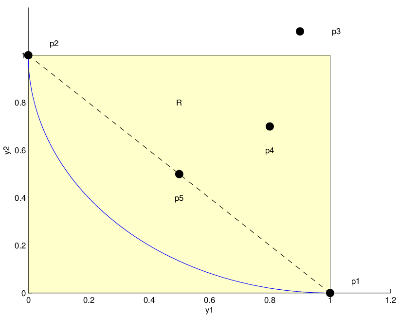
The algorithm for deterministic exploration is shown in Fig. 3. It combines the points used to create a given region in order to produce an initial condition and tries to minimize the distance between its objective value and a reference point. Once a non-dominated point is found, it is returned for exploitation. Although this simple optimization provided good results without requiring many function evaluations, other methods can be used to perform this exploration. Alternatively, one can also perform a stochastic exploration instead of a deterministic one, but this may have negative effects on the performance if the information provided by the output (region R) is not used, since a global search would be required.
The first region is created by finding points that minimize each objective separately, as shown in Fig. 4. This establishes that the initial region will have a number of candidate solutions associated with it equal to the number of objectives, so that the solutions are at the border of the region.
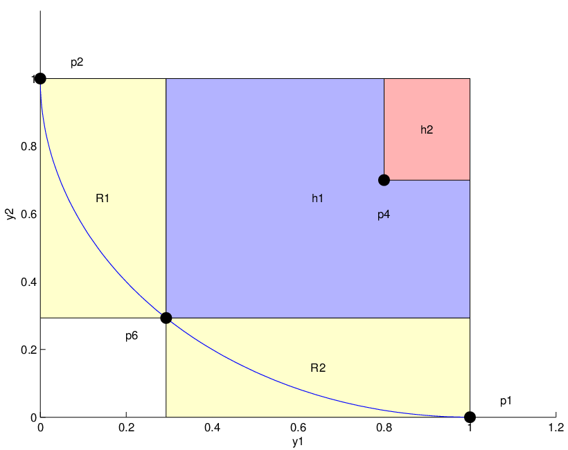
When new regions are created after exploitation, we ignore the solutions that created the region, one at a time, and replace it with the proposed new solution, as shown in Fig. 5, to create a new region. This guarantees that the number of solutions for each region is kept equal to the number of objectives.
Finally, Fig. 6 shows how a region is created. If a region does not have a volume, then at least one objective for two solutions is the same. Although we could allow such region to exist without modifying the rest of the algorithm, these regions tend to not provide good candidates for exploitation and delay the change to stochastic global exploration. Furthermore, one can even prohibit regions with volume smaller than some known constant, as they probably will not provide good exploitation points, and the change to stochastic global exploration happens earlier.
Fig. 7 shows a step of the algorithm in an example problem with two objectives. The deterministic exploration receives a region , composed of the points and . The mean of the points that compose the region is given by and its evaluation in the objective space is shown in Fig. 7(a). The mean objective of the points that compose the region is also computed and is shown as . The deterministic exploration is then defined by the problem
| (3) |
which uses as the initial condition for the optimization. Since is guaranteed to be non-dominated by and , this should guide the search to the non-dominated region of the space.
While performing this optimization, some intermediary points are evaluated, either while computing the numeric gradient or after performing a gradient descent step. The deterministic exploration stops as soon as a non-dominated point is found, which is given by in the example in Fig. 7(a). Note that this example shows as being dominated by and , but it can also be non-dominated. In this case, and no optimization step for the problem in Eq. (3) is performed. Supposing no non-dominated point is found during the deterministic exploration, the region is simply discarded, without performing an exploitation step.
Using the point , whose is non-dominated, provided by the deterministic or stochastic exploration, the exploitation is performed. Fig. 7(b) shows the hypervolume contributions for the initial point and the optimal point , which maximizes the total hypervolume as in Eq. (2). Since is non-dominated, its hypervolume contribution is positive and the hypervolume gradient relative to the objectives is non-zero. After finding and if was provided by the deterministic exploration, new regions must be created to allow further exploration. Therefore, according to Fig. 5, the regions and are created for further exploration.
This finalizes a step of the algorithm, which is repeated until the given stop condition is not met. As at most one point is found by each step, the stop condition can be defined based on the number of desired points.
Note that all the methods used in this algorithm assume that the optimization, either for exploitation or for minimizing one objective alone, requires an initial condition. This is true for hill climbing or gradient methods, but the algorithm can easily be modified if the optimization does not require it.
IV Experimental Results


To compare the algorithm proposed in Section III, called Hybrid Hypervolume Maximization Algorithm (H2MA), with the existing algorithms, the ZDT family of functions [14] was chosen. These functions define a common benchmark set in the multi-objective optimization literature, since they define a wide range of problems to test different characteristics of the optimization algorithm. All functions defined in [14] have a continuous decision space , except for the ZDT5 which has a binary space. In this paper, only the continuous test functions were used to evaluate the performance of the new algorithm, and their equations are shown in the appendix.
Table I provides a summary of the evaluation functions, their decision spaces, and the Nadir points used to compute the hypervolume. The Nadir points are defined by upper bounds of the objectives, which guarantees that the hypervolume computation is always valid, plus one, since not adding an extra value would mean that points at the border of the frontier would have no contribution to the hypervolume and would be avoided. In all instances, a total of variables were considered, as common in the literature. The evolutionary algorithms’ and evaluation functions’ implementations were given by the PaGMO library [16].


| Problem | Objectives | Nadir point | |
|---|---|---|---|
| ZDT1 | Eq. (4) | ||
| ZDT2 | Eq. (5) | ||
| ZDT3 | Eq. (6) | ||
| ZDT4 | Eq. (7) | ||
| ZDT6 | Eq. (8) |
We compare our algorithm with existing state-of-the-art multi-objective optimization algorithms, namely NSGA-II [3], SPEA2 [4], and SMS-EMOA [8]. All of them used a population size of 100 individuals. Tests have shown that this size is able to provide a good performance due to balance between exploration of the space and exploitation of the individuals, with much less individuals not providing good exploration and much more not providing good exploitation. The SMS-EMOA can use two methods for selecting points in dominated fronts: the least hypervolume contribution or the domination count. Both methods were tested, with labels SMS1 and SMS2, respectively, in the following figures. Note that this method only applies for the dominated fronts, since the domination count is zero for all points in the non-dominated front and the least contributor method must be used. Furthermore, the SMS-EMOA algorithm’s performance presented in this paper uses a dynamic Nadir point, which is found by adding one to the maximum over all points in each objective, since using the Nadir points presented in Table I created a very high selective pressure, which in turn led to poor exploration and performance.
Since the decision space and objectives are continuous, the exploitation and deterministic exploration methods may resort to a gradient-based algorithm. In this paper, we used the L-BFGS-B method implemented in the library SciPy [17], which is able to handle the bounds of and is very efficient to find a local optimum. As the other algorithms being compared are evolutionary algorithms, which can only access the objective functions by evaluating them at given points, the gradient for the L-BFGS-B is computed numerically to avoid an unfair advantage in favor of our algorithm.
For the stochastic global exploration, we used an evolutionary algorithm with non-dominance sorting and removal based on the number of dominating points. The population had a minimum size of and was filled with the given set of previous solutions . If less than points were provided, the others were created by randomly sampling the decision space uniformly. Once a new point is introduced to the non-dominated front, it is returned for exploitation because it increases the hypervolume when added to the previous solutions . The size of this population was chosen experimentally to provide a good enough exploration of the space toward the initial conditions for the exploitation. This size is smaller than the population size for the pure evolutionary algorithms because the pure evolutionary algorithm need diversity to explore and exploit all of its population, but the stochastic part of the H2MA is already initialized with good and diverse candidate solutions provided by the exploitation procedure, reducing its exploration requirements.
Besides computing the solutions’ hypervolume, which is the metric that the H2MA is trying to maximize and that provides a good method for comparing solutions, we can compute the distance between the achieved objectives and the Pareto frontier, since the Pareto frontiers for the ZDT functions are known. This defines the P-distance, which is zero, or close to zero due to numerical issues, for points at the frontier.
Figs. 8, 9, 10, 11, and 12 present the results for the problems ZDT1, ZDT2, ZDT3, ZDT4, and ZDT6, respectively. A maximum of 20000 function evaluations was considered, and the graphs show the th, th, th, th, and th percentiles for each performance indicator over 100 runs of the algorithms. Since the P-distance is shown in log-scale, some values obtained by our proposal are absent or partially present, because they have produced zero P-distance.
From ZDT1 to ZDT4, the H2MA never ran out of regions to explore, so the stochastic exploration was not used and all runs have the same performance. For the function ZDT6, the first objective, given by Eq. (8a), causes some problems to the deterministic exploration.
During the creation of the first region for this problem, the mean point is used as initial condition for optimizing each objective, as shown in Fig. 4. However, the first objective for ZDT6 has null derivative when . In this case, even traditional higher-order methods would not help, since the first non-zero derivative of is the sixth. As the first objective does not change in this case and it also has local minima that are very hard to overcome, the algorithm quickly switches to using stochastic exploration. Once new regions have candidate points, the algorithm is able to exploit them.
Besides this issue in the deterministic exploration of the problem ZDT6, the local minima of the first objective makes some candidate solutions be sub-optimal, increasing the P-distance as shown in Fig. 12(b). Nonetheless, the achieved P-distance is better than the evolutionary algorithms and the th percentile is zero. Moreover, Figs. 8(b), 9(b), 10(b), and 11(b) show that the candidate solutions are always on the Pareto frontier for the problems ZDT1 to ZDT4. This allows the user to stop the optimization at any number of evaluations, even with very few function evaluations, and have a reasonable expectation that the solutions found are efficient.
When we evaluate the hypervolume indicator, we see that, for the problems ZDT1, ZDT2, ZDT4, and ZDT6, the performance of the H2MA is much better, even for the last one using stochastic exploration. Moreover, the H2MA’s worst hypervolume was always better than the best hypervolume for all evolutionary algorithms and it was able to get closer to the maximum hypervolume possible with relatively few function evaluations, being a strong indication of its efficiency.
For the problem ZDT3, whose hypervolume performance is shown in Fig. 10(a), the H2MA was generally better than the evolutionary algorithms. The Pareto frontier for ZDT3 is composed of disconnected sets of points, which was created to test the algorithm’s ability to deal with discontinuous frontiers. Since the exploitation algorithm used for the results is gradient-based, it is not able to properly handle discontinuous functions, which is the case of the hypervolume on discontinuous frontiers. However, the deterministic exploration method is able to find points whose exploitation lay on the different parts of the Pareto frontier, providing the expected diversity.

Fig. 13 shows a comparison between the number of function evaluations required by the numeric and the analytic gradient to achieve the same hypervolume on the problems ZDT1 to ZDT4. The analytic method for computing the hypervolume’s gradient is described in [12]. The comparison for ZDT6 is not shown due to its different scale, since many function evaluations are used in the global stochastic exploration because the deterministic exploration fails to find regions.
As expected, using the analytic gradient causes a 30-fold improvement in comparison to the numeric gradient, since the number of decision variables is 30. However, the gain is not linear. This can be explained by the difference in behavior during the deterministic exploration: the first non-dominated point found is used to perform the exploitation, even if this point was found during the computation of the numeric gradient. For ZDT1 and ZDT4, this causes the new points found by the numeric gradient to be very close to the original points, reducing its performance and increasing the improvement of using the analytic gradient.
Moreover, a similar effect makes the ZDT3 performance to have a lower improvement when using the analytic gradient. Since the Pareto frontier for ZDT3 is discontinuous and this causes a discontinuity in the hypervolume, these large changes can be seen by the numeric gradient because small changes in the variables can have large effects on the hypervolume, pulling the solution if the difference is significant, while the analytic gradient is not able to provide such knowledge. Nonetheless, the analytic gradient presents at least a 15-fold improvement over the numeric one over the ZDT3.
IV-A Analysis of the H2MA’s performance
As shown in Section IV, the proposed H2MA is able to surpass the state-of-the-art in multi-objective optimization, based on evolutionary algorithms. Therefore, it is important to analyze the algorithm and to discuss why this improvement happened.
Evolutionary algorithms perform a guided exploration, with new individuals created based on existing high-performing individuals, which allows them to escape local minima but reduces the convergence speed. On the other hand, traditional optimization algorithms tend to find local minima quickly, but the optimal point achieved depends on the minima’s regions of attraction.
These two kind of algorithms have complementary natures, which makes them good candidates for creating a hybrid algorithm: the evolutionary algorithm explores the space and provides initial conditions for the local optimization, which then finds minima quickly. Although this does create better results, it only explains the performance on the ZDT6 problem, since the other problems did not enter the stochastic phase.
In order to understand the algorithm’s behavior, we must keep in mind that each new point added by the algorithm is solving a very different problem. Since the previous points that are considered during the hypervolume optimization change as more points are added, the objective surface for each new point is different from the previous ones and takes into account the already achieved portion of the hypervolume. To visualize this, supposed that the hypervolume’s gradient is defined over previously found points and one previous solution is used as the initial condition for the gradient-based exploitation to find a new point to be added to the solution set. Although the initial condition was a local optimum for a previous problem, it is not a local optimum to the current problem, because any small change that creates a non-dominated point will improve the total hypervolume. Therefore, we do not need to worry about the new optimization converging to a previous solution point because the problem landscape is different and different local minima will be found, increasing the total hypervolume. The deterministic exploration is only required because the hypervolume’s gradient is not defined at the border of the hypervolume, so a new independent point must be found.
This explains the performance improvement over ZDT1 to ZDT4, because every added point improves the hypervolume as much as it can do locally, so that an improvement is guaranteed to happen. Evolutionary algorithms, on the other hand, use function evaluations without guarantees of improvement of the total hypervolume, since dominated solutions can be found.
Moreover, although a local optimum found during exploitation may not be an efficient solution due to irregularities in the objective surface, the experiments show that this is not the case most of the time, since the P-distance of the solutions found are generally zero. This result is expected, since the hypervolume is maximal when computed over points in the Pareto set, and the performance on all ZDT problems provide support to this claim.
We must highlight that we are not saying that evolutionary algorithms should not be used at all, but that they should be applied whenever traditional optimization methods are not able to solve the problem. This is the case of the ZDT6, for instance, where an evolutionary algorithm was required to provide initial conditions for the exploitation. We consider very important to have alternative methods that are better on a subset of the problems and to use them when a problem from such subset is present. This is exactly what the H2MA does: when the traditional optimization is not able to find an answer, which indicates that the problem is outside of the subset with which it can deal, an evolutionary algorithm, which is able to handle a superset class of problems, is used until the problem becomes part of the subset again, establishing a switching behavior that takes advantage of both algorithms.
V Conclusion
This paper proposed the Hybrid Hypervolume Maximization Algorithm (H2MA) for multi-objective optimization, which tries to maximize the hypervolume one point at a time. It first tries to perform deterministic local exploration and, when it gets stuck, it switches to stochastic global exploration using an evolutionary algorithm. The optimization algorithm used during deterministic optimization is problem-dependent and can be given by a gradient-based method, when the decision space is continuous, or a hill-climbing method, when the decision space is discrete. Here we have explored solely continuous decision spaces.
The algorithm was compared with state-of-the-art algorithms for multi-objective optimization, namely NSGA-II, SPEA2, and SMS-EMOA on the ZDT problems. Despite using numeric gradient for the objective functions, which increases the number of function calls, the algorithm consistently provided a higher hypervolume for the same number of function evaluations when compared to the aforementioned evolutionary algorithms. Only for the ZDT3 the performance was slightly reduced due to the discontinuous nature of the Pareto frontier, which causes a discontinuity in the hypervolume, not properly handled by gradient-based methods.
Moreover, for all problems except for ZDT6, all the solutions found by the algorithm were over the Pareto frontier, which makes them efficient solutions. For the ZDT6, the median case also had all solutions over the Pareto frontier, but the use of the stochastic exploration not always guided to a solution at the Pareto frontier. Nonetheless, the obtained solutions were better than those provided by the evolutionary algorithms. Moreover, the solutions provided for ZDT1 to ZDT4 achieved high performance using only the deterministic part of the algorithm.
Evolutionary algorithms usually have better performance when their populations are larger, so that diverse individuals can be selected for crossover. However, most of the time people do not require many options, so the H2MA presents itself as an alternative choice for finding a good set of solutions at a lower computational cost in most problems, although it does not limit the computational burden and the number of points found. If the problem has more reasonable objectives than ZDT6, which was designed with an extreme case in mind, we can expect that many points will be found by the deterministic mechanisms, which makes the algorithm more reliable. Moreover, the solutions found should be efficient, which is characterized by a low P-distance, and diverse on the objectives, which is characterized by a larger hypervolume when only efficient solutions are considered.
Future work should focus on using surrogates to reduce the number of evaluations [18, 19, 20]. Although the H2MA is very efficient on its evaluations, the numeric gradient may consume lots of evaluations and be unreliable for complicated functions, as their implementation can cause numerical errors larger than the step used. Using a surrogate, the gradient can be determined directly and less evaluations are required.
Another important research problem is to find a new algorithm for computing the hypervolume, since existing algorithms are mainly focused on computing the hypervolume given a set of points [21]. Since the solution set is constructed one solution at a time in the H2MA, a recursive algorithm that computes the hypervolume of given the hypervolume of should reduce the computing requirement.
ZDT1:
| (4a) | ||||
| (4b) | ||||
| (4c) | ||||
| (4d) | ||||
ZDT2:
| (5a) | ||||
| (5b) | ||||
| (5c) | ||||
| (5d) | ||||
ZDT3:
| (6a) | ||||
| (6b) | ||||
| (6c) | ||||
| (6d) | ||||
ZDT4:
| (7a) | ||||
| (7b) | ||||
| (7c) | ||||
| (7d) | ||||
ZDT6:
| (8a) | ||||
| (8b) | ||||
| (8c) | ||||
| (8d) | ||||
Acknowledgment
The authors would like to thank CNPq for the financial support.
References
- [1] K. Miettinen, Nonlinear Multiobjective Optimization. Springer US, 1999.
- [2] K. Deb, Multi-Objective Optimization Using Evolutionary Algorithms. John Wiley & Sons, 2001.
- [3] K. Deb, A. Pratap, S. Agarwal, and T. A. M. T. Meyarivan, “A fast and elitist multiobjective genetic algorithm: NSGA-II,” Evolutionary Computation, IEEE Transactions on, vol. 6, no. 2, pp. 182–197, 2002.
- [4] E. Zitzler, M. Laumanns, and L. Thiele, “SPEA2: Improving the strength Pareto evolutionary algorithm,” 2001.
- [5] E. Zitzler, D. Brockhoff, and L. Thiele, “The hypervolume indicator revisited: On the design of Pareto-compliant indicators via weighted integration,” in Evolutionary multi-criterion optimization. Springer, 2007, pp. 862–876.
- [6] E. Zitzler, L. Thiele, M. Laumanns, C. M. Fonseca, and V. G. Da Fonseca, “Performance Assessment of Multiobjective Optimizers: An Analysis and Review,” Evolutionary Computation, IEEE Transactions on, vol. 7, no. 2, pp. 117–132, 2003.
- [7] A. Auger, J. Bader, D. Brockhoff, and E. Zitzler, “Theory of the hypervolume indicator: optimal -distributions and the choice of the reference point,” in Proceedings of the tenth ACM SIGEVO workshop on Foundations of genetic algorithms. ACM, 2009, pp. 87–102.
- [8] N. Beume, B. Naujoks, and M. Emmerich, “SMS-EMOA: Multiobjective selection based on dominated hypervolume,” European Journal of Operational Research, vol. 181, no. 3, pp. 1653–1669, 2007.
- [9] D. Bertsekas, Nonlinear programming. Athena Scientific, 1999.
- [10] D. Luenberger and Y. Ye, Linear and Nonlinear Programming. Springer US, 2008.
- [11] P. A. N. Bosman, “On gradients and hybrid evolutionary algorithms for real-valued multiobjective optimization,” Evolutionary Computation, IEEE Transactions on, vol. 16, no. 1, pp. 51–69, 2012.
- [12] M. Emmerich and A. Deutz, “Time Complexity and Zeros of the Hypervolume Indicator Gradient Field,” in EVOLVE-A Bridge between Probability, Set Oriented Numerics, and Evolutionary Computation III. Springer, 2014, pp. 169–193.
- [13] V. A. S. Hernández, O. Schütze, and M. Emmerich, “Hypervolume Maximization via Set Based Newton’s Method,” in EVOLVE-A Bridge between Probability, Set Oriented Numerics, and Evolutionary Computation V. Springer, 2014, pp. 15–28.
- [14] E. Zitzler, K. Deb, and L. Thiele, “Comparison of Multiobjective Evolutionary Algorithms: Empirical Results,” Evolutionary Computation, vol. 8, no. 2, pp. 173–195, 2000.
- [15] K. Deb, “Multi-objective optimization,” in Search methodologies. Springer, 2014, pp. 403–449.
- [16] F. Biscani, D. Izzo, and C. H. Yam, “A global optimisation toolbox for massively parallel engineering optimisation,” arXiv preprint arXiv:1004.3824, 2010.
- [17] E. Jones, T. Oliphant, P. Peterson et al., “SciPy: Open source scientific tools for Python,” 2001–, [Online; accessed 2015-05-10]. [Online]. Available: http://www.scipy.org/
- [18] Y. Jin, “A Comprehensive Survey of Fitness Approximation in Evolutionary Computation,” Soft computing, vol. 9, no. 1, pp. 3–12, 2005.
- [19] J. Knowles and H. Nakayama, “Meta-Modeling in Multiobjective Optimization,” in Multiobjective Optimization. Springer, 2008, pp. 245–284.
- [20] I. Voutchkov and A. Keane, “Multi-objective Optimization Using Surrogates,” in Computational Intelligence in Optimization. Springer, 2010, pp. 155–175.
- [21] N. Beume, C. M. Fonseca, M. López-Ibáñez, L. Paquete, and J. Vahrenhold, “On the complexity of computing the hypervolume indicator,” Evolutionary Computation, IEEE Transactions on, vol. 13, no. 5, pp. 1075–1082, 2009.
| Conrado S. Miranda received his M.S. degree on Mechanical Engineering and his B.S. in Control and Automation Engineering from the University of Campinas (Unicamp), Brazil, in 2014 and 2011, respectively. He is currently a Ph.D. student at the School of Electrical and Computer Engineering, Unicamp. His main research interests are machine learning, multi-objective optimization, neural networks, and statistical models. |
![[Uncaptioned image]](1506.05424v1/FernandoVonZuben_reduced.png) |
Fernando J. Von Zuben received his Dr.E.E. degree from the University of Campinas (Unicamp), Campinas, SP, Brazil, in 1996. He is currently the header of the Laboratory of Bioinformatics and Bioinspired Computing (LBiC), and a Full Professor at the Department of Computer Engineering and Industrial Automation, School of Electrical and Computer Engineering, University of Campinas (Unicamp). The main topics of his research are computational intelligence, natural computing, multivariate data analysis, and machine learning. He coordinates open-ended research projects in these topics, tackling real-world problems in the areas of information technology, decision-making, pattern recognition, and discrete and continuous optimization. |