跳到论文正文
W Papers独立论文阅读器 arXiv:1506.05412 论文正文 计算阅读时间 · 0%
引用这篇论文根据当前论文元数据生成,正式投稿前建议核对。


License: arXiv.org perpetual non-exclusive license
arXiv:1506.05412v2 [hep-th] 01 Oct 2015

A test of bosonization at the level of four-point functions in Chern-Simons vector models

Akshay Bedhotiya Email: aksbed@gmail.com    and Shiroman Prakash Affiliation: Dayalbagh Educational Institute, Agra, India Email: shiroman@gmail.com
Abstract

We study four-point functions in Chern-Simons vector models in the large NN limit. We compute the four-point function of the scalar primary to all orders in the ‘t Hooft coupling λ=N/k\lambda=N/k in U​(N)kU(N)_{k} Chern-Simons theory coupled to a fundamental fermion, in both the critical and non-critical theory, for a particular case of the external momenta. These theories cover the entire 3-parameter "quasi-boson" and 2-parameter "quasi-fermion" families of 3-dimensional quantum field theories with a slightly-broken higher spin symmetry. Our results are consistent with the celebrated bosonization duality, as we explicitly verify by calculating four-point functions in the free critical and non-critical bosonic theories.

1 Introduction

U​(N)kU(N)_{k} Chern-Simons theories coupled to fundamental matter provide an interesting class of interacting three-dimensional conformal field theories that are exactly solvable in the ’t Hooft limit: N→∞N\rightarrow\infty, k→∞k\rightarrow\infty with the ’t Hooft coupling λ≡Nk\lambda\equiv\frac{N}{k} held fixed. These theories, which have been intensively studied in the past few years [1, 2, 3, 4, 5, 6, 7, 8, 9, 10, 11, 12, 13], are particularly interesting because they provide examples of non-supersymmetric dualities. For instance, they are widely believed to be dual to Vasiliev higher-spin gauge theories (see [14] for a review.) They also exhibit a spectacular bosonization duality relating Chern-Simons theory coupled to fundamental fermions to critical Chern-Simons theory coupled to fundamental bosons, which can be thought of as a non-supersymmetric generalisation of the ABJ and Giveon-Kutasov dualities. [1, 2, 3, 4, 5, 6, 7, 8, 10, 15, 16, 17]

The bosonization duality has been tested via three point functions and also in thermal free energy computations, leaving little doubt to its correctness. However, it is still of independent interest to directly test the duality at the level of four-point functions; which are not determined by purely kinematic considerations.

In this paper, we calculate four-point correlation functions of the primary scalar operator J(0)J^{(0)} in the critical and non-critical U​(N)kU(N)_{k} Chern-Simons theory coupled to fundamental fermions. For a particular choice of external momenta, we are able to obtain a closed form (but highly non-trivial) expression for the four point function of the scalar primary as a function of λ\lambda – which we then compare to the free and critical bosonic theories to obtain another independent check of the bosonization duality.

1.1 Review of the Bosonization Duality

The bosonization duality [3], which can be thought of as a non-supersymmetric generalization of the Giveon-Kutasov duality [16], states that a U​(Nf)kfU(N_{f})_{k_{f}} Chern-Simons theory coupled to fermions in the fundamental representation is dual to a U​(Nb)kbU(N_{b})_{k_{b}} Chern-Simons theory coupled to critical bosons in the fundamental representation. The critical theory is obtained by deforming the usual (non-critical) theory by a double trace operator λ4​ϕ2​ϕ2\lambda_{4}\phi^{2}\phi^{2} and taking the coupling to infinity. (The coupling λ4\lambda_{4} should not be confused with λb=Nb/kb\lambda_{b}=N_{b}/k_{b}.)

The conjectured duality claims that the two theories are equivalent, with the following relation between parameters:

kf=−kb\displaystyle k_{f}=-k_{b} (1)
Nf=|kb|−Nb\displaystyle N_{f}=|k_{b}|-N_{b} (2)

Though we present the duality in terms of kk and NN, the duality has only been tested in the large NN, ’t Hooft limit; at finite NN there will be some shifts of ±1/2\pm 1/2 in the Chern-Simons level for the fermionic theory as discussed in [3, 4]. All parameters are defined in a dimensional reduction regularization scheme, used in [3]. In terms of λ=Nk\lambda=\frac{N}{k}, the duality can be written as:

λf=λb− sign⁡(λb),\displaystyle\lambda_{f}=\lambda_{b}-\sign(\lambda_{b}), (3)
Nf=Nb​1−|λ|b|λ|b,\displaystyle N_{f}=N_{b}\frac{1-|\lambda|_{b}}{|\lambda|_{b}}, (4)

or

λb=λf− sign⁡(λf),\displaystyle\lambda_{b}=\lambda_{f}-\sign(\lambda_{f}), (5)
Nb=Nf​1−|λ|f|λ|f.\displaystyle N_{b}=N_{f}\frac{1-|\lambda|_{f}}{|\lambda|_{f}}. (6)

From these results, we have the simple relation |λb|=1−|λf||\lambda_{b}|=1-|\lambda_{f}| and  sign⁡(λb)=− sign⁡(λf)\sign(\lambda_{b})=-\sign(\lambda_{f}).

As both sides of the theory are exactly solvable, the simplest way to verify the duality is to calculate correlation functions on both sides, which we illustrate below.

The two-point function of the scalar primary, which is defined as Jf0≡ψ¯​ψJ_{f}^{0}\equiv\bar{\psi}\psi, in the fermionic theory is:

⟨Jf0​(−q)​Jf0⟩=−Nf​tan⁡(π​λf/2)4​π​λf​|q|.\displaystyle\langle J_{f}^{0}(-q)J_{f}^{0}\rangle=-N_{f}\frac{\tan(\pi\lambda_{f}/2)}{4\pi\lambda_{f}}|q|. (7)

In the critical bosonic theory, the two-point function is:

⟨Jb0​(−q)​Jb0⟩=−Nb​4​π​λbtan⁡(π​λb/2)​|q|.\displaystyle\langle J_{b}^{0}(-q)J_{b}^{0}\rangle=-N_{b}\frac{4\pi\lambda_{b}}{\tan(\pi\lambda_{b}/2)}|q|. (8)

These two-point functions determine the relative normalisation of the scalar operator in the two descriptions. We see that, taking Jb0=4​π​λb​Jf0J_{b}^{0}=4\pi\lambda_{b}J_{f}^{0}11 1 This relation makes sense because λ\lambda and Jf0J_{f}^{0} are odd under parity, while Jb0J_{b}^{0} is even., the two point functions are identical:

⟨Jb0​(−q)​Jb0⟩=−Nb​4​π​λbtan⁡(π​λb/2)​|q|\displaystyle\langle J_{b}^{0}(-q)J_{b}^{0}\rangle=-N_{b}\frac{4\pi\lambda_{b}}{\tan(\pi\lambda_{b}/2)}|q|
⟨Jf0​(−q)​Jf0⟩=−Nb​cot⁡(π​λb/2)4​π​λb​|q|\displaystyle\langle J_{f}^{0}(-q)J_{f}^{0}\rangle=-N_{b}\frac{\cot(\pi\lambda_{b}/2)}{4\pi\lambda_{b}}|q|
=Nf​ sign⁡(λb)​tan⁡(π​λf/2)4​π​(1−|λb|)​|q|\displaystyle=N_{f}\sign(\lambda_{b})\frac{\tan(\pi\lambda_{f}/2)}{4\pi(1-|\lambda_{b}|)}|q|
=−Nf​tan⁡(π​λf/2)4​π​λf​|q|\displaystyle=-N_{f}\frac{\tan(\pi\lambda_{f}/2)}{4\pi\lambda_{f}}|q|

The duality now implies that, for the three-point functions:

⟨Jf0​(q1)​Jf0​(q2)​Jf0​(q3)⟩=(14​π​λb)3​⟨Jb0​(q1)​Jb0​(q2)​Jb0​(q3)⟩\displaystyle\langle J_{f}^{0}(q_{1})J_{f}^{0}(q_{2})J_{f}^{0}(q_{3})\rangle=\left(\frac{1}{4\pi\lambda_{b}}\right)^{3}\langle J_{b}^{0}(q_{1})J_{b}^{0}(q_{2})J_{b}^{0}(q_{3})\rangle (9)

Using the results in [3, 4], we can explicitly compute that:

⟨Jf0​(q1)​Jf0​(q2)​Jf0​(q3)⟩=0\displaystyle\langle J_{f}^{0}(q_{1})J_{f}^{0}(q_{2})J_{f}^{0}(q_{3})\rangle=0
⟨Jb0​(q1)​Jb0​(q2)​Jb0​(q3)⟩=0\displaystyle\langle J_{b}^{0}(q_{1})J_{b}^{0}(q_{2})J_{b}^{0}(q_{3})\rangle=0

which agrees with the duality,.

There are additional predictions for three-point functions; for instance for the three-point function of vector and scalar operators, which are non-zero, and which can be tested on similar lines.

Applying the duality to four-point functions, we obtain:

(4​π​(λf− sign⁡(λf)))4​⟨Jf0​(q1)​Jf0​(q2)​Jf0​(q3)​Jf0​(q4)⟩\displaystyle\hskip-8.53581pt\left(4\pi\left(\lambda_{f}-\sign(\lambda_{f})\right)\right)^{4}\left\langle J_{f}^{0}(q_{1})J_{f}^{0}(q_{2})J_{f}^{0}(q_{3})J_{f}^{0}(q_{4})\right\rangle =\displaystyle= ⟨Jb0​(q1)​Jb0​(q2)​Jb0​(q3)​Jb0​(q4)⟩\displaystyle\left\langle J_{b}^{0}(q_{1})J_{b}^{0}(q_{2})J_{b}^{0}(q_{3})J_{b}^{0}(q_{4})\right\rangle (10)

In what follows, we directly calculate the LHS of (10) (for a restricted class of external momenta) and obtain a finite answer in the limit λf→1\lambda_{f}\rightarrow 1 (when expressed in terms of NbN_{b}). The result can then be compared to a calculation the critical bosonic theory at λb=0\lambda_{b}=0 on the RHS and we find perfect agreement.

As described below, and in [3, 4], the non-critical bosonic theory is dual to a critical fermionic theory. We also compare the critical fermionic theory to the non-critical bosonic theory and find agreement.

2 The Exact Ladder Diagram

Refer to caption
Figure 1: The diagrammatic definition of the exact ladder diagram, which is the shaded box. All propagators in this diagram are exact propagators. In light cone gauge, this diagram is sufficient to calculate all planar correlation functions of single trace operators.

In this paper, we will exclusively use light-cone gauge22 2 The conventions used in the following sections are those of [1, 3, 4]. In particular, our light-cone gauge is defined in Euclidean space and described in detail in [1]. We also use the notation that γA\gamma^{A} may be the 2×22\times 2 identity matrix 𝟏\mathbf{1} or any of the three γμ\gamma^{\mu} and ps2=p12+p22=2​p+​p−p_{s}^{2}=p_{1}^{2}+p_{2}^{2}=2p_{+}p_{-}.. Two crucial features of light-cone gauge are that ghosts decouple and cubic vertices are absent. Therefore any planar correlation function can be evaluated to all orders in λ\lambda given the exact propagator, first evaluated in [1], and the "exact ladder diagram" defined diagrammatically in Figure 1, which we denote by ΓA​B​(p,q,r)​γA⊗γB\Gamma_{AB}(p,q,r)\gamma^{A}\otimes\gamma^{B}.

More precisely, we define ΓA​B​(p,q,r)​γA⊗γB\Gamma_{AB}(p,q,r)\gamma^{A}\otimes\gamma^{B} as the following four-fermion interaction term in the quantum effective action for fermions, obtained after integrating out the gauge field in light cone gauge.

Se​f​f=−12∫d3​p​d3​q​d3​r(2​π)9ΓA​B(p,q,r)ψ¯i(−p)γAψj(r)ψ¯j(−r−q)γBψi(p+q).S_{eff}=-\frac{1}{2}\int\frac{d^{3}pd^{3}qd^{3}r}{(2\pi)^{9}}\Gamma_{AB}(p,q,r)\bar{\psi}^{i}(-p)\gamma^{A}\psi_{j}(r)\bar{\psi}^{j}(-r-q)\gamma^{B}\psi_{i}(p+q). (11)

S⁡(p)S(p), the exact large NN fermion propagator, valid to all orders in λ\lambda, is defined via ⟨ψi​(p)​ψ¯j​(q)⟩=δij​(2​π)3​δ3​(p−q)​S​(p)\langle\psi_{i}(p)\bar{\psi}^{j}(q)\rangle=\delta_{i}^{j}(2\pi)^{3}\delta^{3}(p-q)S(p) and is given by [1]:

S⁡(p)=(−i​γμ​pμ+i​λ2​γ+​p−+λ​psp2).S(p)=\left({-i\gamma^{\mu}p_{\mu}+i\lambda^{2}\gamma^{+}p^{-}+\lambda p_{s}\over p^{2}}\right). (12)

The gauge propagator is defined via ⟨Aμ​(p)​Aν​(−q)⟩=δa​b​(2​π)3​δ3​(p−q)​Gν​μ​(p)\langle A_{\mu}(p)A_{\nu}(-q)\rangle=\delta^{ab}(2\pi)^{3}\delta^{3}(p-q)G_{\nu\mu}(p) and is given by

G+3=4​π​ik​1p+.G_{+3}=\frac{4\pi i}{k}\frac{1}{p^{+}}. (13)

The self-consistent Schwinger-Dyson equation, given diagrammatically in Figure 1, where all propagators are taken to be exact propagators S⁡(p)S(p), is:

ΓA​B​(p,q,r)​γA⊗γB=(−2​π​ik)​1(p−r)+​(γ+⊗γ3−γ3⊗γ+)\displaystyle\Gamma_{AB}(p,q,r)\gamma^{A}\otimes\gamma^{B}=\left(\frac{-2\pi i}{k}\right)\frac{1}{(p-r)^{+}}\left(\gamma^{+}\otimes\gamma^{3}-\gamma^{3}\otimes\gamma^{+}\right)
+(−2​N​π​ik)∫d3​l(2​π)31l+ΓC​D(l,q,r)\displaystyle+\left(\frac{-2N\pi i}{k}\right)\int\frac{d^{3}l}{(2\pi)^{3}}\frac{1}{l^{+}}\Gamma_{CD}(l,q,r)
×(γ+​S​(l)​γC⊗γD​S​(l+q)​γ3−γ3​S​(l)​γC⊗γD​S​(l+q)​γ+).\displaystyle\times\left(\gamma^{+}S(l)\gamma^{C}\otimes\gamma^{D}S(l+q)\gamma^{3}-\gamma^{3}S(l)\gamma^{C}\otimes\gamma^{D}S(l+q)\gamma^{+}\right). (14)

In terms of S⁡(p)=SA​(p)​γAS(p)=S_{A}(p)\gamma^{A}, we have:

ΓA​B​(p,q,r)​γA⊗γB=(−2​π​ik)​1(p−r)+​(γ+⊗γ3−γ3⊗γ+)\displaystyle\Gamma_{AB}(p,q,r)\gamma^{A}\otimes\gamma^{B}=\left(\frac{-2\pi i}{k}\right)\frac{1}{(p-r)^{+}}\left(\gamma^{+}\otimes\gamma^{3}-\gamma^{3}\otimes\gamma^{+}\right)
−(2λπi)∫d3​l(2​π)31l+ΓC​D(l,q,r)SE(l)SF(l+q)\displaystyle-\left(2\lambda\pi i\right)\int\frac{d^{3}l}{(2\pi)^{3}}\frac{1}{l^{+}}\Gamma_{CD}(l,q,r)S_{E}(l)S_{F}(l+q)
×(γ+​γF​γC⊗γD​γE​γ3−γ3​γF​γC⊗γD​γE​γ+)\displaystyle\times\left(\gamma^{+}\gamma^{F}\gamma^{C}\otimes\gamma^{D}\gamma^{E}\gamma^{3}-\gamma^{3}\gamma^{F}\gamma^{C}\otimes\gamma^{D}\gamma^{E}\gamma^{+}\right) (15)

2.1 Rewriting the Schwinger-Dyson equation

There are 16 components of ΓA​B\Gamma_{AB}, which appear to be coupled. We now obtain an alternate expression for ΓA​B\Gamma_{AB} that “diagonalizes” the Schwinger-Dyson equation (15) and shows that most of the 16 components are not independent.

For this purpose it is convenient to define:

4πiAP(p,q,r)QγP=ΓA​B(p,q,r)γAγQγB.4\pi iA_{P}{}^{Q}(p,q,r)\gamma^{P}=\Gamma_{AB}(p,q,r)\gamma^{A}\gamma^{Q}\gamma^{B}. (16)

It is easy to see that the inverse relation is

4πi Tr(γAγPγBγQ)AP(p,q,r)Q=ΓA​B(p,q,r)4\pi i\text{ Tr}\left(\gamma_{A}\gamma^{P}\gamma_{B}\gamma_{Q}\right)A_{P}{}^{Q}(p,q,r)=\Gamma_{AB}(p,q,r) (17)

(where ‘Tr’ denotes a trace over the gamma matrices.)

Let us also define, following [1]

H+​(Y)=γ3​Y​γ+−γ+​Y​γ3=2​(YI​γ+−Y−​I).H_{+}(Y)=\gamma^{3}Y\gamma^{+}-\gamma^{+}Y\gamma^{3}=2(Y_{I}\gamma^{+}-Y_{-}I). (18)

The Schwinger-Dyson equation (15) can be re-written as

4πiAP(p,q,r)QγP\displaystyle 4\pi iA_{P}{}^{Q}(p,q,r)\gamma^{P} =\displaystyle= ΓA​B​(p,q,r)​γA​γQ​γB\displaystyle\Gamma_{AB}(p,q,r)\gamma^{A}\gamma^{Q}\gamma^{B} (20)
=\displaystyle= (−2​π​ik)​1(p−r)+​(γ+​γQ​γ3−γ3​γQ​γ+)\displaystyle\left(\frac{-2\pi i}{k}\right)\frac{1}{(p-r)^{+}}\left(\gamma^{+}\gamma^{Q}\gamma^{3}-\gamma^{3}\gamma^{Q}\gamma^{+}\right)
+(−2​N​π​ik)∫d3​l(2​π)3ll+ΓC​D(l,q,r)SE(l)SF(l+q)\displaystyle+\left(\frac{-2N\pi i}{k}\right)\int\frac{d^{3}l}{(2\pi)^{3}}\frac{l}{l^{+}}\Gamma_{CD}(l,q,r)S_{E}(l)S_{F}(l+q)
×(γ+​γF​γC​γQ​γD​γE​γ3−γ3​γF​γC​γQ​γD​γE​γ+)\displaystyle\times\left(\gamma^{+}\gamma^{F}\gamma^{C}\gamma^{Q}\gamma^{D}\gamma^{E}\gamma^{3}-\gamma^{3}\gamma^{F}\gamma^{C}\gamma^{Q}\gamma^{D}\gamma^{E}\gamma^{+}\right)
=\displaystyle= (2​π​ik)​1(p−r)+​H+​(γQ)\displaystyle\left(\frac{2\pi i}{k}\right)\frac{1}{(p-r)^{+}}H_{+}(\gamma^{Q})
+(2​N​π​ik)∫d3​l(2​π)31l+ΓC​D(l,q,r)SE(l)SF(l+q)×\displaystyle+\left(\frac{2N\pi i}{k}\right)\int\frac{d^{3}l}{(2\pi)^{3}}\frac{1}{l^{+}}\Gamma_{CD}(l,q,r)S_{E}(l)S_{F}(l+q)\times
H+​(γF​γC​γQ​γD​γE)\displaystyle H_{+}(\gamma^{F}\gamma^{C}\gamma^{Q}\gamma^{D}\gamma^{E}) (21)
AP(p,q,r)QγP\displaystyle A_{P}{}^{Q}(p,q,r)\gamma^{P} =\displaystyle= (12​k)​1(p−r)+​H+​(γQ)\displaystyle\left(\frac{1}{2k}\right)\frac{1}{(p-r)^{+}}H_{+}(\gamma^{Q}) (22)
+2πiλ∫d3​l(2​π)31l+AP(l,q,r)QSE(l)SF(l+q)×\displaystyle+2\pi i\lambda\int\frac{d^{3}l}{(2\pi)^{3}}\frac{1}{l^{+}}A_{P}{}^{Q}(l,q,r)S_{E}(l)S_{F}(l+q)\times
H+​(γF​γP​γE)\displaystyle H_{+}(\gamma^{F}\gamma^{P}\gamma^{E})

Because H+H_{+} contains only the identity and γ+\gamma^{+} components,this means that

A3(p,q,r)Q=A−(p,q,r)Q=0A_{3}{}^{Q}(p,q,r)=A_{-}{}^{Q}(p,q,r)=0 (23)

for all QQ. This translates into 88 linear equations relating various of the 16 components of ΓA​B\Gamma_{AB}. Moreover, the 8 A+QA_{+}{}^{Q} and AIQA_{I}{}^{Q} are the only non-vanishing components of AA, and they are independent for different values of QQ. It is also consistent to set AP3=0A_{P}{}^{3}=0 and AP+=0A_{P}{}^{+}=0 so we have only 4 equations, which are 2 pairs of 2 coupled integral equations.

Evaluating (22) explicitly, we obtain:

A+(p,q,r)Qγ++AI(p,q,r)Q\displaystyle A_{+}{}^{Q}(p,q,r)\gamma^{+}+A_{I}{}^{Q}(p,q,r) =\displaystyle= (12​k)​1(p−r)+​H+​(γQ)\displaystyle\left(\frac{1}{2k}\right)\frac{1}{(p-r)^{+}}H_{+}(\gamma^{Q}) (24)
+2πiλ∫d3​l(2​π)31l+A+(l,q,r)QSE(l)SF(l+q)×H+(γFγ+γE)\displaystyle\hskip-56.9055pt+2\pi i\lambda\int\frac{d^{3}l}{(2\pi)^{3}}\frac{1}{l^{+}}A_{+}{}^{Q}(l,q,r)S_{E}(l)S_{F}(l+q)\times H_{+}(\gamma^{F}\gamma^{+}\gamma^{E})
+2πiλ∫d3​l(2​π)31l+AI(l,q,r)QSE(l)SF(l+q)×H+(γFγE)\displaystyle\hskip-56.9055pt+2\pi i\lambda\int\frac{d^{3}l}{(2\pi)^{3}}\frac{1}{l^{+}}A_{I}{}^{Q}(l,q,r)S_{E}(l)S_{F}(l+q)\times H_{+}(\gamma^{F}\gamma^{E})

2.2 Evaluating the exact ladder diagram when q±=0q_{\pm}=0

We have not yet been able to solve this integral equation for arbitrary qq. However, if we restrict ourselves to q±=0q_{\pm}=0 it is possible to obtain a solution, which will enable us to calculate the four-point function of scalar primaries for a restricted class external momenta.

To motivate our ansatz for the solution, we note that the results of section 2.1 can also be thought of diagrammatically as follows: Let f(0)​(p,q,r)f^{(0)}(p,q,r) be any 2×22\times 2 matrix (with spinor indices) that is a function of pp, qq and rr. We think of f(0)​δjif^{(0)}\delta^{i}_{j} as representing an arbitrary "contraction" of the ladder diagram on the right, so that the tree level ladder diagram acting on f0​δmlf^{0}\delta^{l}_{m} is given by

N2​γν​f(0)​(p,q,r)​γμ​Gμ​ν​(p−r)​δji=N2​δji​G+3​(p−r)​H+​(f(0)​(p,q,r))\frac{N}{2}\gamma^{\nu}f^{(0)}(p,q,r)\gamma^{\mu}G_{\mu\nu}(p-r)\delta^{i}_{j}=\frac{N}{2}\delta^{i}_{j}G_{+3}(p-r)H_{+}\left(f^{(0)}(p,q,r)\right) (25)

as pictured in Figure 2.

Refer to caption
Figure 2: A contraction of the tree-level ladder diagram corresponding to Equation (25). Note that there is no integration over momenta.

We then define f(n)​(p,q,r)f^{(n)}(p,q,r) (which can be thought of as the ladder diagram with nn "rungs", contracted with f(0)f^{(0)} on the right) recursively in terms of f(n−1)f^{(n-1)}:

γν​f(n)​(p,q,r)​γμ​Gμ​ν​(p−r)=N2​γν​(∫d3​l(2​π)3​S​(l)​γσ​f(n−1)​(l,q,r)​γρ​Gρ​σ​(l−r)​S​(l+q)​Gμ​ν​(p−l))​γμ\gamma^{\nu}f^{(n)}(p,q,r)\gamma^{\mu}G_{\mu\nu}(p-r)=\frac{N}{2}\gamma^{\nu}\left(\int\frac{d^{3}l}{(2\pi)^{3}}S(l)\gamma^{\sigma}f^{(n-1)}(l,q,r)\gamma^{\rho}G_{\rho\sigma}(l-r)S(l+q)G_{\mu\nu}(p-l)\right)\gamma^{\mu} (26)

as pictured in Figure 3.

Refer to caption
Figure 3: The diagrammatic relation for f(n)f^{(n)} in terms of f(n−1)f^{(n-1)}.

Because G+3=−G3+G_{+3}=-G_{3+} are the only nonzero components of Gμ​νG_{\mu\nu}, only two components of f(n−1)f^{(n-1)} contribute to f(n)f^{(n)}, which are

H+​(f(n))=2​fI(n)​γ+−2​f−(n)​𝕀.H_{+}\left(f^{(n)}\right)=2f_{I}^{(n)}\gamma^{+}-2f_{-}^{(n)}\mathbb{I}. (27)

In terms of these variables, the equation (26) is:

H+​(f(n)​(p,q,r))(p−r)+=2​π​i​λ​∫d3​l(2​π)3​H+​(S⁡(l)​H+​(f(n−1)​(l,q,r))​S​(l+q))​1(l−r)+​(p−l)+{H_{+}(f^{(n)}(p,q,r))\over(p-r)^{+}}=2\pi i\lambda\int\frac{d^{3}l}{(2\pi)^{3}}H_{+}\left(S(l)H_{+}\left(f^{(n-1)}(l,q,r)\right)S(l+q)\right)\frac{1}{(l-r)^{+}(p-l)^{+}} (28)

The infinite sum ∑f(n)\sum f^{(n)} is related to APQA_{P}^{Q} defined in (16) of the previous subsection and fI(0)f_{I}^{(0)} and f−(0)f_{-}^{(0)} as follows:

∑fI(n)k​(p−r)+=A+I​fI(0)+A+−​f−(0),−∑f−(n)k​(p−r)+=AII​fI(0)+AI−​f−(0).\frac{\sum f^{(n)}_{I}}{k(p-r)^{+}}=A_{+}^{I}f_{I}^{(0)}+A_{+}^{-}f_{-}^{(0)},~~~-\frac{\sum f^{(n)}_{-}}{k(p-r)^{+}}=A_{I}^{I}f_{I}^{(0)}+A_{I}^{-}f_{-}^{(0)}. (29)

.

Let us choose f(0)f^{(0)} (which is an arbitrary matrix) such that f−(0)=−c​fI(0)​r+f_{-}^{(0)}=-cf_{I}^{(0)}r^{+}. The parameter cc is arbitrary, and introduced for convenience: when we set c=0c=0, equation (29) determines A+IA_{+}^{I} and AIIA_{I}^{I} and when c→+∞c\rightarrow+\infty, equation (29) determines A+−A_{+}^{-} and AI−A_{I}^{-}.

We note that it is consistent to assume f(n)​(p,q,r)f^{(n)}(p,q,r) is independent of p3p_{3}. Evaluating equation (26), including the l3l_{3} integral, we have:

fIn​(p)(p−r)+=−2iλ∫d2​l(2​π)2fIn−1​(l)​(q3+2​i​λ​ls)​l+−f−n−1​(l)​(2​(1−λ2)​ls2)(q32+4​ls2)​ls1(p−l)+​(l−r)+\frac{f_{I}^{n}(p)}{(p-r)^{+}}=-2i\lambda\int\frac{d^{2}l}{(2\pi)^{2}}\frac{f_{I}^{n-1}(l)\left(q_{3}+2i\lambda l_{s}\right)l^{+}-f_{-}^{n-1}(l)\left(2\left(1-\lambda^{2}\right)l_{s}^{2}\right)}{\left(q_{3}^{2}+4l_{s}^{2}\right)l_{s}}\frac{1}{(p-l)^{+}(l-r)^{+}} (30)
f−n​(p)(p−r)+=−2iλ∫d2​l(2​π)2fIn−1​(l)​2​l+2−f−n−1​(l)​(2​i​λ​ls−q3)​l+(q32+4​ls2)​ls1(p−l)+​(l−r)+\hskip-22.76219pt\frac{f_{-}^{n}(p)}{(p-r)^{+}}=-2i\lambda\int\frac{d^{2}l}{(2\pi)^{2}}\frac{f_{I}^{n-1}(l)2l^{+2}-f_{-}^{n-1}(l)\left(2i\lambda l_{s}-q_{3}\right)l^{+}}{\left(q_{3}^{2}+4l_{s}^{2}\right)l_{s}}\frac{1}{(p-l)^{+}(l-r)^{+}} (31)

After integrating to obtain the first few terms, we find fI(n)​(p)f_{I}^{(n)}(p) and f−(n)​(p)f_{-}^{(n)}(p) to be of the form:

fI(n)​(p)=a1(n)+a2(n)​r+p+\displaystyle f_{I}^{(n)}(p)=a_{1}^{(n)}+a_{2}^{(n)}\frac{r^{+}}{p^{+}} (32)
f−(n)​(p)=−b1(n)​p+−b2(n)​r+\displaystyle f_{-}^{(n)}(p)=-b_{1}^{(n)}p^{+}-b_{2}^{(n)}r^{+} (33)

We can sum the series to obtain:

∑fI(n)(p)−fI(0)=−2iλ∫d2​l(2​π)2(∑fIn​(l)​(q3+2​i​λ​ls)​l+−∑f−n​(l)​(2​(1−λ2)​ls2))(q32+4​ls2)​ls(p−r)+(p−l)+​(l−r)+\sum f_{I}^{(n)}(p)-f_{I}^{(0)}=-2i\lambda\int\frac{d^{2}l}{(2\pi)^{2}}\frac{\left(\sum f_{I}^{n}(l)\left(q_{3}+2i\lambda l_{s}\right)l^{+}-\sum f_{-}^{n}(l)\left(2\left(1-\lambda^{2}\right)l_{s}^{2}\right)\right)}{\left(q_{3}^{2}+4l_{s}^{2}\right)l_{s}}\frac{(p-r)^{+}}{(p-l)^{+}(l-r)^{+}} (34)
∑f−(n)(p)−f−(0)=−2iλ∫d2​l(2​π)2(∑fI(n)​(l)​2​l+2−∑f−(n)​(l)​(2​i​λ​ls−q3)​l+)(q32+4​ls2)​ls(p−r)+(p−l)+​(l−r)+\sum f_{-}^{(n)}(p)-f_{-}^{(0)}=-2i\lambda\int\frac{d^{2}l}{(2\pi)^{2}}\frac{\left(\sum f_{I}^{(n)}(l)2l^{+2}-\sum f_{-}^{(n)}(l)\left(2i\lambda l_{s}-q_{3}\right)l^{+}\right)}{\left(q_{3}^{2}+4l_{s}^{2}\right)l_{s}}\frac{(p-r)^{+}}{(p-l)^{+}(l-r)^{+}} (35)

From (32) and (33) we make the ansatz

∑fI(n)​(p)=(a1+a2​r+p+)​fI(0)∑f−(n)​(p)=−(b1​p++b2​r+)​fI(0).\sum f_{I}^{(n)}(p)=\left(a_{1}+a_{2}\frac{r^{+}}{p^{+}}\right)f_{I}^{(0)}\hskip 28.45274pt\sum f_{-}^{(n)}(p)=-\left(b_{1}p^{+}+b_{2}r^{+}\right)f_{I}^{(0)}. (36)

We now use the identity

1(p−l)+​(l−r)+=1(p−r)+​(1(p−l)++1(l−r)+){\frac{1}{(p-l)^{+}(l-r)^{+}}}={\frac{1}{(p-r)^{+}}\left(\frac{1}{(p-l)^{+}}+\frac{1}{(l-r)^{+}}\right)} (37)

and, following [3], introduce the dimensionless variables:

y=2​ps|q3|x=2​rs|q3|t=2​ls|q3|Λ^=2​Λs|q3|λ^=λ​ sign​(q3)\displaystyle y=\frac{2p_{s}}{|q_{3}|}\hskip 14.22636ptx=\frac{2r_{s}}{|q_{3}|}\hskip 14.22636ptt=\frac{2l_{s}}{|q_{3}|}\hskip 14.22636pt\hat{\Lambda}=\frac{2\Lambda_{s}}{|q_{3}|}\hskip 14.22636pt\hat{\lambda}=\lambda\text{ sign}(q_{3}) (38)

to carry out the angular integrals and rewrite (34) and (35) as

((a1+a2​r+p+)−1)\displaystyle\left(\left(a_{1}+a_{2}\frac{r^{+}}{p^{+}}\right)-1\right) =\displaystyle= ∫xy(a1​(1+i​λ^​t)+b12​(1−λ^2)​t2)​𝑑t+∫x0(a2​(1+i​λ​t)+b2)​𝑑t\displaystyle\int_{x}^{y}\left(a_{1}\left(1+i\hat{\lambda}t\right)+\frac{b_{1}}{2}\left(1-\hat{\lambda}^{2}\right)t^{2}\right)\,dt+\int_{x}^{0}\left(a_{2}(1+i\lambda t)+b_{2}\right)\,dt
+r+p+∫0y(a2(1+iλ^t)+b22(1−λ^2)t2)dt\displaystyle+\frac{r^{+}}{p^{+}}\int_{0}^{y}\left(a_{2}\left(1+i\hat{\lambda}t\right)+\frac{b_{2}}{2}\left(1-\hat{\lambda}^{2}\right)t^{2}\right)\,dt (39)
(b1​p++b2​r+)−c​r+=\displaystyle\left(b_{1}p^{+}+b_{2}r^{+}\right)-cr^{+}= r+​(∫xΛ(2​a1+b1​(i​λ^​t−1))​𝑑t+∫xy(2​a2+b2​(i​λ^​t−1))​𝑑t)\displaystyle r^{+}\left(\int_{x}^{\Lambda}\left(2a_{1}+b_{1}\left(i\hat{\lambda}t-1\right)\right)dt\right.\left.+\int_{x}^{y}\left(2a_{2}+b_{2}\left(i\hat{\lambda}t-1\right)\right)\,dt\right)
+p+∫Λy(2a1+b1(iλ^t−1))dt.\displaystyle+p^{+}\int_{\Lambda}^{y}\left(2a_{1}+b_{1}\left(i\hat{\lambda}t-1\right)\right)\,dt. (40)

To solve these coupled four-variable equations (which could in principle have been obtained directly from equation (24) with the approporiate ansatz for APQA_{P}^{Q}) we differentiate and the resulting differential equation decouples into two sets of two variable coupled equations.

Equating coefficients of r+p+,p+\frac{r^{+}}{p^{+}},p^{+} and r+r^{+}, we obtain:

∂a1∂y=−(a1​(1+i​λ^​y)+b12​(1−λ^2)​y2)\displaystyle\frac{\partial a_{1}}{\partial y}=-\left(a_{1}\left(1+i\hat{\lambda}y\right)+\frac{b_{1}}{2}\left(1-\hat{\lambda}^{2}\right)y^{2}\right)
12​∂b1∂y=(a1+b12​(i​λ^​y−1))\displaystyle\frac{1}{2}\frac{\partial b_{1}}{\partial y}=\left(a_{1}+\frac{b_{1}}{2}\left(i\hat{\lambda}y-1\right)\right)
∂a2∂y=−(a2​(1+i​λ^​y)+b2​(1−λ^2)​y2)\displaystyle\frac{\partial a_{2}}{\partial y}=-\left(a_{2}\left(1+i\hat{\lambda}y\right)+b_{2}\left(1-\hat{\lambda}^{2}\right)y^{2}\right)
12​∂b2∂y=(a2+b2​(i​λ^​y−1))\displaystyle\frac{1}{2}\frac{\partial b_{2}}{\partial y}=\left(a_{2}+b_{2}\left(i\hat{\lambda}y-1\right)\right) (41)

The general solution of the set is

ai\displaystyle a_{i} =\displaystyle= αi​(βi​(1−i​λ^​y)−(1+i​λ^​y)​e−2​i​λ^​arctan⁡(y))\displaystyle\alpha_{i}\left(\beta_{i}(1-i\hat{\lambda}y)-(1+i\hat{\lambda}y)e^{-2i\hat{\lambda}\arctan(y)}\right)
bi\displaystyle b_{i} =\displaystyle= 2​αi​(βi+e−2​i​λ^​arctan⁡(y))\displaystyle 2\alpha_{i}\left(\beta_{i}+e^{-2i\hat{\lambda}\arctan(y)}\right) (42)

where the subscript i=1,2i=1,2. Requiring that the solutions satisfy the integral equations (39) and (40) fixes the integration constants:

β1\displaystyle\beta_{1} =\displaystyle= −e−2​i​λ^​arctan⁡[Λ^]\displaystyle-e^{-2i\hat{\lambda}\arctan[\hat{\Lambda}]}
β2\displaystyle\beta_{2} =\displaystyle= 1\displaystyle 1
α1\displaystyle\alpha_{1} =\displaystyle= c2​((1−i​λ^​x)−(1+i​λ^​x)​e−2​i​λ^​arctan⁡[x])−(1+e−2​i​λ^​arctan⁡[x])2​e−2​i​λ^​arctan⁡[x]​(1+e−2​i​λ^​arctan⁡[Λ^])\displaystyle\frac{\frac{c}{2}\left((1-i\hat{\lambda}x)-(1+i\hat{\lambda}x)e^{-2i\hat{\lambda}\arctan[x]}\right)-\left(1+e^{-2i\hat{\lambda}\arctan[x]}\right)}{2e^{-2i\hat{\lambda}\arctan[x]}\left(1+e^{-2i\hat{\lambda}\arctan[\hat{\Lambda}]}\right)}
α2\displaystyle\alpha_{2} =\displaystyle= c2​((1−i​λ^​x)​e−2​i​λ^​arctan⁡[Λ^]+(1+i​λ^​x)​e−2​i​λ^​arctan⁡[x])−(e−2​i​λ^​arctan⁡[Λ^]−e−2​i​λ^​arctan⁡[x])2​e−2​i​λ^​arctan⁡[x]​(1+e−2​i​λ^​arctan⁡(Λ^)).\displaystyle\frac{\frac{c}{2}\left((1-i\hat{\lambda}x)e^{-2i\hat{\lambda}\arctan[\hat{\Lambda}]}+(1+i\hat{\lambda}x)e^{-2i\hat{\lambda}\arctan[x]}\right)-\left(e^{-2i\hat{\lambda}\arctan[\hat{\Lambda}]}-e^{-2i\hat{\lambda}\arctan[x]}\right)}{2e^{-2i\hat{\lambda}\arctan[x]}\left(1+e^{-2i\hat{\lambda}\arctan(\hat{\Lambda})}\right)}. (43)

To determine A+IA_{+}^{I} and AIIA_{I}^{I} we set c=0c=0 and to determine A+−A_{+}^{-} and AI−A_{I}^{-} we take the limit c→∞c\rightarrow\infty (i.e., equate coefficients of cc on both sides of Equation (29)). Writing the answers in the form:

A~CB=2​k​e−2​i​λ^​arctan⁡[x]​(1+e−2​i​λ^​arctan⁡(Λ^))​(p−r)+​ACB\tilde{A}_{C}^{B}=2ke^{-2i\hat{\lambda}\arctan[x]}\left(1+e^{-2i\hat{\lambda}\arctan(\hat{\Lambda})}\right)(p-r)^{+}A_{C}^{B}

we have:

A~II\displaystyle\tilde{A}_{I}^{I} =\displaystyle= (e−2​i​λ^​arctan⁡[Λ^]−e−2​i​λ^​arctan⁡[y])​(1+e−2​i​λ^​arctan⁡[x])​(2​p+q3)\displaystyle\left(e^{-2i\hat{\lambda}\arctan[\hat{\Lambda}]}-e^{-2i\hat{\lambda}\arctan[y]}\right)\left(1+e^{-2i\hat{\lambda}\arctan[x]}\right)\left(\frac{2p^{+}}{q_{3}}\right) (44)
+(e−2​i​λ^​arctan⁡[x]−e−2​i​λ^​arctan⁡[Λ^])​(1+e−2​i​λ^​arctan⁡[y])​(2​r+q3)\displaystyle+\left(e^{-2i\hat{\lambda}\arctan[x]}-e^{-2i\hat{\lambda}\arctan[\hat{\Lambda}]}\right)\left(1+e^{-2i\hat{\lambda}\arctan[y]}\right)\left(\frac{2r^{+}}{q_{3}}\right)
A~I−\displaystyle\tilde{A}_{I}^{-} =\displaystyle= −(e−2​i​λ^​arctan⁡[Λ^]−e−2​i​λ^​arctan⁡[y])​((i​λ^​x−1)+(1+i​λ^​x)​e−2​i​λ^​arctan⁡[x])​(p+r+)\displaystyle-\left(e^{-2i\hat{\lambda}\arctan[\hat{\Lambda}]}-e^{-2i\hat{\lambda}\arctan[y]}\right)\left((i\hat{\lambda}x-1)+(1+i\hat{\lambda}x)e^{-2i\hat{\lambda}\arctan[x]}\right)\left(\frac{p^{+}}{r^{+}}\right) (45)
−((1+i​λ^​x)​e−2​i​λ^​arctan⁡[x]−(i​λ^​x−1)​e−2​i​λ^​arctan⁡[Λ^])​(1+e−2​i​λ^​arctan⁡[y])\displaystyle-\left((1+i\hat{\lambda}x)e^{-2i\hat{\lambda}\arctan[x]}-(i\hat{\lambda}x-1)e^{-2i\hat{\lambda}\arctan[\hat{\Lambda}]}\right)\left(1+e^{-2i\hat{\lambda}\arctan[y]}\right)
A~+I\displaystyle\tilde{A}_{+}^{I} =\displaystyle= ((1+i​λ^​y)​e−2​i​λ^​arctan⁡[y]−(i​λ^​y−1)​e−2​i​λ^​arctan⁡[Λ^])​(1+e−2​i​λ^​arctan⁡[x])\displaystyle\left((1+i\hat{\lambda}y)e^{-2i\hat{\lambda}\arctan[y]}-(i\hat{\lambda}y-1)e^{-2i\hat{\lambda}\arctan[\hat{\Lambda}]}\right)\left(1+e^{-2i\hat{\lambda}\arctan[x]}\right) (46)
+(e−2​i​λ^​arctan⁡[Λ^]−e−2​i​λ^​arctan⁡[x])​((i​λ^​y−1)+(1+i​λ^​y)​e−2​i​λ^​arctan⁡[y])​(r+p+)\displaystyle+\left(e^{-2i\hat{\lambda}\arctan[\hat{\Lambda}]}-e^{-2i\hat{\lambda}\arctan[x]}\right)\left((i\hat{\lambda}y-1)+(1+i\hat{\lambda}y)e^{-2i\hat{\lambda}\arctan[y]}\right)\left(\frac{r^{+}}{p^{+}}\right)
A~+−\displaystyle\hskip-8.53581pt\tilde{A}_{+}^{-} =\displaystyle= −((1+iλ^y)e−2​i​λ^​arctan⁡[y]−(iλ^y−1)e−2iλ^arctan[Λ^]])\displaystyle-\left((1+i\hat{\lambda}y)e^{-2i\hat{\lambda}\arctan[y]}-(i\hat{\lambda}y-1)e^{-2i\hat{\lambda}\arctan[\hat{\Lambda}]]}\right) (47)
×(((1+i​λ^​x)​e−2​i​λ^​arctan⁡[x]+(i​λ^​x−1))​(q32​r+))\displaystyle\times\left(\left((1+i\hat{\lambda}x)e^{-2i\hat{\lambda}\arctan[x]}+(i\hat{\lambda}x-1)\right)\left(\frac{q_{3}}{2r^{+}}\right)\right)
−((i​λ^​x−1)​e−2​i​λ^​arctan⁡[Λ^]−(1+i​λ^​x)​e−2​i​λ^​arctan⁡[x])\displaystyle-\left((i\hat{\lambda}x-1)e^{-2i\hat{\lambda}\arctan[\hat{\Lambda}]}-(1+i\hat{\lambda}x)e^{-2i\hat{\lambda}\arctan[x]}\right)
×((i​λ^​y−1)+(1+i​λ^​y)​e−2​i​λ^​arctan⁡[y])​(q32​p+)\displaystyle\times\left((i\hat{\lambda}y-1)+(1+i\hat{\lambda}y)e^{-2i\hat{\lambda}\arctan[y]}\right)\left(\frac{q_{3}}{2p^{+}}\right)

In Appendix A, we evaluate the exact vertex for the scalar primary using this result.

3 Four-Point Correlation Functions

We now proceed to calculate the (gauge-invariant and parity-invariant) four-point function of the scalar primary. In this section, we evaluate the four-point function in the free fermionic theory, the interacting fermionic theory and the critical interacting fermionic theory. In section 4, we then evaluate the four-point function in the free and critical bosonic theories to test the duality. The four-point functions depend on external momenta q(i)q^{(i)}; as discussed in the previous section, our calculations are only valid in the special case of q±=0q_{\pm}=0 (i.e., only q3≠0q_{3}\neq 0). Hence, in what follows, we drop all spacetime-indices and label the four external momenta as q1q_{1}, q2q_{2}, q3q_{3} and q4q_{4}.

3.1 Free Fermionic Theory

The free (λf=0\lambda_{f}=0) four-point function in the U⁡(Nf)U(N_{f}) fermionic theory is given by

F⁡(q1,q2,q3,q4)\displaystyle F(q_{1},q_{2},q_{3},q_{4}) =\displaystyle= ⟨J(0)​(−q1)​J(0)​(−q2)​J(0)​(−q3)​J(0)​(−q4)⟩\displaystyle\langle J^{(0)}(-q_{1})J^{(0)}(-q_{2})J^{(0)}(-q_{3})J^{(0)}(-q_{4})\rangle (48)
=\displaystyle= −Nf∫d3​k(2​π)3 Tr(S0(k)S0(k+q1)S0(k+q1+q2)S0(k+q1+q2+q3))\displaystyle-N_{f}\int\frac{d^{3}k}{(2\pi)^{3}}\text{ Tr}\left(S_{0}(k)S_{0}(k+q_{1})S_{0}(k+q_{1}+q_{2})S_{0}(k+q_{1}+q_{2}+q_{3})\right)
+ permutations\displaystyle+\text{ permutations}

where S0​(q)=(i​q̸)−1S_{0}(q)=(i\not{q})^{-1} is the free fermion propagator and all external momenta are restricted in the 3 direction.

Evaluating this, we obtain

F⁡(q1,q2,q3,q4)=Nf​18​(q1+q2)​(q1+q4)​(∣q1∣−∣q2​∣+∣q3∣−∣​q4∣)+5 permutationsF(q_{1},q_{2},q_{3},q_{4})=N_{f}\frac{1}{8(q_{1}+q_{2})(q_{1}+q_{4})}(\mid q_{1}\mid-\mid q_{2}\mid+\mid q_{3}\mid-\mid q_{4}\mid)+\text{5 permutations} (49)

which can be simplified to:

F⁡(q1,q2,q3,q4)=Nf​q1​|q1|+q2​|q2|+q3​|q3​|+q4|​q4|2​(q1+q2)​(q1+q3)​(q2+q3)​δ​(q1+q2+q3+q4)F(q_{1},q_{2},q_{3},q_{4})=N_{f}\frac{q_{1}|q_{1}|+q_{2}|q_{2}|+q_{3}|q_{3}|+q_{4}|q_{4}|}{2(q_{1}+q_{2})(q_{1}+q_{3})(q_{2}+q_{3})}\delta(q_{1}+q_{2}+q_{3}+q_{4}) (50)

3.2 Interacting Fermionic Theory

We now proceed to calculate the four-point function in the interacting theory.

In the interacting theory, our basic ingredients are the exact propagator, the exact J(0)J^{(0)} vertex VV [4], and the ladder diagram in section 2. The correlator can be written as as a sum of Diagrams AA, BB and CC in Figure 4 (where it is understood that all propagators are exact),

⟨J(0)​(p−q)​J(0)​(−t)​J(0)​(t−p)​J(0)​(q)⟩=[A]+[B]+[C].\langle J^{(0)}(p-q)J^{(0)}(-t)J^{(0)}(t-p)J^{(0)}(q)\rangle=[\text{A}]+[\text{B}]+[\text{C}]. (51)

The diagrams BB and CC involve the ladder diagram.

Diagram AA is given by

(A)=−N∫d3​k(2​π)3Tr[V(p−q)S(k)V(−t)S(k+t)V(t−p)S(k+p)V(q)S(k+p−q)]\displaystyle(\text{A})=-N\int\frac{d^{3}k}{(2\pi)^{3}}\text{Tr}\left[V(p-q)S(k)V(-t)S(k+t)V(t-p)S(k+p)V(q)S(k+p-q)\right]
+(5​ permutations)\displaystyle+(5\text{ permutations}) (52)

and diagrams BB and CC are given by

(B)\displaystyle(\text{B}) =\displaystyle= N∫d3​k(2​π)3Tr[S(r+p)V(q)S(r−p+q)V(p−q)S(r)γμS(k)V(−t)S(k+t)V(t−p)\displaystyle N\int\frac{d^{3}k}{(2\pi)^{3}}\text{Tr}[S(r+p)V(q)S(r-p+q)V(p-q)S(r)\gamma^{\mu}S(k)V(-t)S(k+t)V(t-p)
S(k+p)γνΓμ​ν(k,p,r)]+(5 permutations)\displaystyle S(k+p)\gamma^{\nu}\Gamma_{\mu\nu}(k,p,r)]+(5\text{ permutations}) (53)
(C)\displaystyle(\text{C}) =\displaystyle= N∫d3​k(2​π)3Tr[(S(r+p−q−t)V(p−q)S(r−t)V(−t)S(r)γμS(k)V(t−p)S(k+p−t)\displaystyle N\int\frac{d^{3}k}{(2\pi)^{3}}\text{Tr}[(S(r+p-q-t)V(p-q)S(r-t)V(-t)S(r)\gamma^{\mu}S(k)V(t-p)S(k+p-t)
V(q)S(k+p−q−t)γνΓμ​ν(k,p−q−t,r)]+(5 permutations)\displaystyle V(q)S(k+p-q-t)\gamma^{\nu}\Gamma_{\mu\nu}(k,p-q-t,r)]+(5\text{ permutations}) (54)

It is difficult to solve this integral in closed from for arbitrary pp, qq, and tt. To obtain humanly readable answers that can be easily compared to the bosonic theory, we observe that the limit where two momenta (q→0+q\rightarrow 0^{+} and t→0+t\rightarrow 0^{+} ) vanish is relatively tractable.

Let us first consider the diagrams where the two non-vanishing external momenta are “diagonal" (as depicted in Figure 4 when q→0+q\rightarrow 0^{+} and t→0+t\rightarrow 0^{+}). In this limit, the integral is solvable. We find the 2 “diagonal" permutations of diagram AA are given by

−N∫d3​k(2​π)3Tr[V(p−q)S(k)V(−t)S(k+t)V(t−p)S(k+p)V(q)S(k+q)]\displaystyle-N\int\frac{d^{3}k}{(2\pi)^{3}}\text{Tr}[V(p-q)S(k)V(-t)S(k+t)V(t-p)S(k+p)V(q)S(k+q)]
=−N​sec⁡(π​λ2)2​(π​λ+sin⁡(π​λ))4​(2​π​λ​|p|)\displaystyle=-N\frac{\sec(\frac{\pi\lambda}{2})^{2}(\pi\lambda+\sin(\pi\lambda))}{4(2\pi\lambda|p|)} (55)

For diagrams BB and CC, we use (29)and (44)-(45) for the ladder expressions, and obtain

2 permutations of B=N​sec3⁡(π​λ2)​(2​π​λ​cos⁡(π​λ2)−7​sin⁡(π​λ2)+sin⁡(3​π​λ2))32​p​π​λ\text{2 permutations of B}=N\sec^{3}\left(\frac{\pi\lambda}{2}\right)\frac{(2\pi\lambda\cos\left(\frac{\pi\lambda}{2}\right)-7\sin\left(\frac{\pi\lambda}{2}\right)+\sin\left(\frac{3\pi\lambda}{2}\right))}{32p\pi\lambda} (56)

Adding (55) and (56) for B as well as C gives

−N​2​sec2⁡(π​λ2)​tan⁡(π​λ2)4​|p|​π​λ-N\frac{2\sec^{2}\left(\frac{\pi\lambda}{2}\right)\tan\left(\frac{\pi\lambda}{2}\right)}{4|p|\pi\lambda} (57)
Refer to caption
Figure 4: Diagrams in the interacting theory.

The next step is to evaluate the remaining permutations of diagrams AA, BB and CC with two adjacent non-vanishing external momenta (i.e., permutations of the external momenta not depicted in Figure 44). These integrals are more nontrivial, but can be obtained by using the substitution q→p−qq\rightarrow p-q in (52) and (54) which evaluates to

−N​1|p|​(sec2⁡(π​λ2)​tan⁡(π​λ2)4​π​λ+h⁡(λ))-N\frac{1}{|p|}\left(\frac{\sec^{2}\left(\frac{\pi\lambda}{2}\right)\tan\left(\frac{\pi\lambda}{2}\right)}{4\pi\lambda}+h(\lambda)\right) (58)

where h⁡(λ)h(\lambda) is

h⁡(λ)=i4​(1+ei​π​λ)2​(1+2​ei​π​λ​π​λ​cot⁡(π​λ)+λ​ψ​(1−λ2)−λ​ψ​(−λ2)+CLOSE\displaystyle h(\lambda)=\frac{i}{4\left(1+e^{i\pi\lambda}\right)^{2}}\Big(1+2e^{i\pi\lambda}\pi\lambda\cot\left(\pi\lambda\right)+\lambda\psi\left(\frac{1-\lambda}{2}\right)-\lambda\psi\left(\frac{-\lambda}{2}\right)+
OPENe2​i​π​λ​(1+λ​ψ​(λ2)−λ​ψ​(1+λ2)))\displaystyle e^{2i\pi\lambda}\left(1+\lambda\psi\left(\frac{\lambda}{2}\right)-\lambda\psi\left(\frac{1+\lambda}{2}\right)\right)\Big) (59)

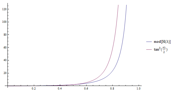
and ψ⁡(x)=Γ′​(x)Γ⁡(x)\psi(x)=\frac{\Gamma^{\prime}(x)}{\Gamma(x)} is the Digamma function. It can be seen that the above equation goes to 0 for λ→0\lambda\rightarrow 0 and decreases approximately as −tan2⁡(π​λ2)-\tan^{2}(\frac{\pi\lambda}{2}). This property will be later be of use in the critical theory.

In summary, after adding all the diagrams we get the following result

⟨J(0)​(p−q)​J(0)​(−t)​J(0)​(t−p)​J(0)​(q)⟩=−N​2​sec2⁡(π​λ2)​tan⁡(π​λ2)|p|​π​λ−4​N​h​(λ)|p|\langle J^{(0)}(p-q)J^{(0)}(-t)J^{(0)}(t-p)J^{(0)}(q)\rangle=-N\frac{2\sec^{2}\left(\frac{\pi\lambda}{2}\right)\tan\left(\frac{\pi\lambda}{2}\right)}{|p|\pi\lambda}-\frac{4Nh(\lambda)}{|p|} (60)
Refer to caption
Figure 5: The plot of modulus of H⁡(p,λ)H(p,\lambda) function and tan3⁡[π​λ2]\tan^{3}[\frac{\pi\lambda}{2}] vs λ\lambda for momenta p=1p=1. It is clear that the magnitude of H⁡(λ)H(\lambda) rises slower than tan3⁡[π​λ2]\tan^{3}[\frac{\pi\lambda}{2}].

It is worthwhile to notice that both terms in the R.H.S of (60) are parity invariant. We can draw a parallel between (49) ,(50) and (57) ,(60) respectively.

It is natural to conjecture that this expression generalises to the following expression for general momenta:

⟨J(0)​(−q1)​J(0)​(−q2)​J(0)​(−q3)​J(0)​(−q4)⟩=2​sec2⁡(π​λ2)​tan⁡(π​λ2)π​λ​F​(q1,q2,q3,q4)\displaystyle\langle J^{(0)}(-q_{1})J^{(0)}(-q_{2})J^{(0)}(-q_{3})J^{(0)}(-q_{4})\rangle=\frac{2\sec^{2}\left(\frac{\pi\lambda}{2}\right)\tan\left(\frac{\pi\lambda}{2}\right)}{\pi\lambda}F(q_{1},q_{2},q_{3},q_{4})
+H⁡(q1,q2,q3,q4,λ)\displaystyle+H(q_{1},q_{2},q_{3},q_{4},\lambda) (61)

where F⁡(q1,q2,q3,q4)F(q_{1},q_{2},q_{3},q_{4}) is the four-point function of the scalar operator in the free fermionic theory and H⁡(q1,q2,q3,q4,λ)H(q_{1},q_{2},q_{3},q_{4},\lambda) is an additional structure, which goes to zero as λ→0\lambda\rightarrow 0.

3.3 Critical Fermionic Theory

We now consider the four point function of the scalar primary in the critical fermionic theory described in [3], [4], which is conjectured to be dual to the (non-critical) bosonic theory.

Let us briefly review the definition of the critical fermonic theory, which at zero-coupling is essentially the Gross-Neveu model (in three-dimensions): We introduce a field σ\sigma (without a kinetic term) that couples to the scalar primary as Sσ=∫d3​x​σ​ψ¯​ψS_{\sigma}=\int d^{3}x\sigma\bar{\psi}\psi and perform a path integral over σ\sigma. The equation of motion for σ\sigma is ψ¯​ψ=0\bar{\psi}\psi=0; therefore, instead of ψ¯​ψ\bar{\psi}\psi, the single trace scalar primary operator in the critical theory is σ\sigma. Notice that, ψ¯​ψ\bar{\psi}\psi has scaling dimension 2, so σ\sigma has scaling dimension 11, which matches the scaling dimension of the scalar primary Jb(0)=ϕ¯​ϕJ^{(0)}_{b}=\bar{\phi}\phi in the non-critical bosonic theory, as required for a duality. Because σ\sigma has mass dimension 11, there is the possibility of an additional marginal coupling of the form ∫d3​x​N​λ6F3!​σ3\int d^{3}xN\frac{\lambda^{F}_{6}}{3!}\sigma^{3}, which is related to the marginal ϕ6\phi^{6} coupling in the bosonic theory.

In the large NN limit, the exact two point function of σ\sigma is clearly related the inverse of the two point function of ψ¯​ψ\bar{\psi}\psi, via

G⁡(q)=⟨σ⁡(−q)​σ⟩=(−⟨Jf(0)​(−q)​Jf(0)⟩non-critical)−1,G(q)=\langle\sigma(-q)\sigma\rangle=\left(-\langle J^{(0)}_{f}(-q)J^{(0)}_{f}\rangle_{\text{non-critical}}\right)^{-1}, (62)

where two-point function of the scalar primary Jf(0)J_{f}^{(0)} in the non-critical theory is

⟨Jf(0)​(−q)​Jf(0)⟩=−Nf​tan⁡(π​λf2)4​π​λf​|q|.\langle J_{f}^{(0)}(-q)J_{f}^{(0)}\rangle=-\frac{N_{f}\tan\left(\frac{\pi\lambda_{f}}{2}\right)}{4\pi\lambda_{f}}|q|. (63)
Refer to caption Refer to caption Refer to caption
Figure 6: The diagrams that contribute to the four-point function of σ\sigma in the critical fermionic theory. The shaded square is the exact scalar four-point function in the non-critical theory, the shaded triangle is the exact three-point function in the non-critical theory and the dashed line with a shaded circle is the ⟨σ​σ⟩\langle\sigma\sigma\rangle propagator. The last diagram includes the contribution from the marginal λ6\lambda_{6} coupling, represented by black dot. (There is also another diagram with only one λ6\lambda_{6} vertex and one exact three point function that is not pictured.)

Directly using the result (61), it is not hard to calculate the four-point function of the scalar primary operator σ\sigma in the critical fermionic theory. The diagrams that contribute to the four-point function of σ\sigma are shown in Figure 6.

⟨σ^​(−q1)​σ^​(−q2)​σ^​(−q3)​σ^​(−q4)⟩=N4​λ~q.b4​G​(−q1)​G​(−q2)​G​(−q3)​G​(−q4)\displaystyle\langle\hat{\sigma}(-q_{1})\hat{\sigma}(-q_{2})\hat{\sigma}(-q_{3})\hat{\sigma}(-q_{4})\rangle=N^{4}\tilde{\lambda}_{q.b}^{4}G(-q_{1})G(-q_{2})G(-q_{3})G(-q_{4})
(⟨J(0)​(−q1)​J(0)​(−q2)​J(0)​(−q3)​J(0)​(−q4)⟩+CLOSE\displaystyle(\langle J^{(0)}(-q_{1})J^{(0)}(-q_{2})J^{(0)}(-q_{3})J^{(0)}(-q_{4})\rangle+
G⁡(q1+q2)​(⟨J(0)​(−q1)​J(0)​(−q2)​J(0)​(q1+q2)⟩​⟨J(0)​(−q3)​J(0)​(−q4)​J(0)​(q3+q4)⟩+CLOSE\displaystyle G(q_{1}+q_{2})(\langle J^{(0)}(-q_{1})J^{(0)}(-q_{2})J^{(0)}(q_{1}+q_{2})\rangle\langle J^{(0)}(-q_{3})J^{(0)}(-q_{4})J^{(0)}(q_{3}+q_{4})\rangle+
OPENOPENλ6​(⟨J(0)​(−q1)​J(0)​(−q2)​J(0)​(q1+q2)⟩+⟨J(0)​(−q3)​J(0)​(−q4)​J(0)​(q3+q4)⟩)+λ62))+ permutations\displaystyle\lambda_{6}(\langle J^{(0)}(-q_{1})J^{(0)}(-q_{2})J^{(0)}(q_{1}+q_{2})\rangle+\langle J^{(0)}(-q_{3})J^{(0)}(-q_{4})J^{(0)}(q_{3}+q_{4})\rangle)+\lambda_{6}^{2}))+\text{ permutations} (64)

The critical fermionic theory is dual to the non-critical bosonic theory in the limit λf→1\lambda_{f}\rightarrow 1 and λ6=0\lambda_{6}=0. In this limit, there are two surviving terms in (64), the first two diagrams of Figure 6. Using (61) and the fermionic three point function [4] we find

⟨σ^(−q1)σ^(−q2)σ^(−q3)σ^(−q4)⟩=−256​π4​λf4​cot8⁡(π​λf2)|q1|​|q2​‖q3‖​q4|×\displaystyle\langle\hat{\sigma}(-q_{1})\hat{\sigma}(-q_{2})\hat{\sigma}(-q_{3})\hat{\sigma}(-q_{4})\rangle=-\frac{256\pi^{4}\lambda_{f}^{4}\cot^{8}\left(\frac{\pi\lambda_{f}}{2}\right)}{|q_{1}||q_{2}||q_{3}||q_{4}|}\times
(2​sec2⁡(π​λf2)​tan⁡(π​λf2)π​λ​F​(q1,q2,q3,q4)+H⁡(q1,q2,q3,q4)CLOSE\displaystyle\Big(\frac{2\sec^{2}\left(\frac{\pi\lambda_{f}}{2}\right)\tan\left(\frac{\pi\lambda_{f}}{2}\right)}{\pi\lambda}F(q_{1},q_{2},q_{3},q_{4})+H(q_{1},q_{2},q_{3},q_{4})
OPEN+Nf​tan3⁡(π​λf2)π​λf​(1|q1+q2|+1|q1+q3|+1|q3+q3|))\displaystyle+\frac{N_{f}\tan^{3}\left(\frac{\pi\lambda_{f}}{2}\right)}{\pi\lambda_{f}}\left(\frac{1}{|q_{1}+q_{2}|}+\frac{1}{|q_{1}+q_{3}|}+\frac{1}{|q_{3}+q_{3}|}\right)\Big) (65)
=−256​π4​λf4|q1|​|q2​‖q3‖​q4|​cot4⁡(π​λf2)​|λb||λf|​(F⁡(q1,q2,q3,q4)+Nf​(12​|q1+q2|+12​|q1+q3|+12​|q3+q3|))\displaystyle=-\frac{256\pi^{4}\lambda_{f}^{4}}{|q_{1}||q_{2}||q_{3}||q_{4}|}\cot^{4}\left(\frac{\pi\lambda_{f}}{2}\right)\frac{|\lambda_{b}|}{|\lambda_{f}|}\left(F(q_{1},q_{2},q_{3},q_{4})+N_{f}\left(\frac{1}{2|q_{1}+q_{2}|}+\frac{1}{2|q_{1}+q_{3}|}+\frac{1}{2|q_{3}+q_{3}|}\right)\right) (66)

In the last step we have applied the limit λf→1\lambda_{f}\rightarrow 1 and used (6) to express the answer in terms of |λb||\lambda_{b}|, anticipating the comparison in the next section. We have also used the fact that H⁡(q1,q2,q3,q4)∼tan2⁡(π​λf2)H(q_{1},q_{2},q_{3},q_{4})\sim\tan^{2}\left(\frac{\pi\lambda_{f}}{2}\right) to eliminate it from (66). Using equation (70), this expression can be compared to the four-point correlator of J^b(0)\hat{J}^{(0)}_{b} in the bosonic theory which we calculate in the next section.

4 Comparison to the Bosonic Theory

4.1 Non-Critical Bosonic Theory

In the free theory, we have

⟨J(0)​(−q1)​J(0)​(−q2)​J(0)​(−q3)​J(0)​(−q4)⟩\displaystyle\langle J^{(0)}(-q_{1})J^{(0)}(-q_{2})J^{(0)}(-q_{3})J^{(0)}(-q_{4})\rangle (67)
=N​∫d3​k(2​π)3​1k2​(k+q1)2​(k+q1+q2)2​(k+q1+q2+q3)2\displaystyle\hskip-85.35826pt=N\int\frac{d^{3}k}{(2\pi)^{3}}\frac{1}{k^{2}(k+q_{1})^{2}(k+q_{1}+q_{2})^{2}(k+q_{1}+q_{2}+q_{3})^{2}} (68)

We solve (68) in the limit q±=0q_{\pm}=0. The integral evaluates to

N2((q22+q32+q1​q2+q1​q3+q2​q3)|q1|​q2​q3​(q1+q2+q3)​(q1+q2)​(q1+q3)​(q2+q3)+(q1→q2,q3)\displaystyle\frac{N}{2}\Big(\frac{(q_{2}^{2}+q_{3}^{2}+q_{1}q_{2}+q_{1}q_{3}+q_{2}q_{3})}{|q_{1}|q_{2}q_{3}(q_{1}+q_{2}+q_{3})(q_{1}+q_{2})(q_{1}+q_{3})(q_{2}+q_{3})}+(q_{1}\rightarrow q_{2},q_{3})
+q1​q2+q1​q3+q2​q3q1​q2​q3​|q1+q2+q3|​(q1+q2)​(q1+q3)​(q2+q3)\displaystyle+\frac{q_{1}q_{2}+q_{1}q_{3}+q_{2}q_{3}}{q_{1}q_{2}q_{3}|q_{1}+q_{2}+q_{3}|(q_{1}+q_{2})(q_{1}+q_{3})(q_{2}+q_{3})}
−(q1+q3)​(q2+q3)(q1​q2​q3​(q1+q2+q3)​|(q1+q2)|​(q1+q3)​(q2+q3))+(q1↔q2↔q3)))\displaystyle-\frac{(q_{1}+q_{3})(q_{2}+q_{3})}{(q_{1}q_{2}q_{3}(q_{1}+q_{2}+q_{3})|(q_{1}+q_{2})|(q_{1}+q_{3})(q_{2}+q_{3}))}+(q_{1}\leftrightarrow q_{2}\leftrightarrow q_{3}))\Big) (69)

where the arrows in the numerator imply symmetric terms on replacing q1q_{1} with q2q_{2} and q3q_{3}.

Refer to caption
Figure 7: Correction to the critical scalar four correlator.

Using the normalisation relation

σ^=−4​π​λf​cot⁡(π​λf2)​Jb(0)\hat{\sigma}=-4\pi\lambda_{f}\cot\left(\frac{\pi\lambda_{f}}{2}\right)J^{(0)}_{b} (70)

which follows from comparing the two point functions of the scalar primaries in both theories, it is easy to see that this result matches the R.H.S of (66) – i.e., that

⟨σ⁡(−q1)​σ​(−q2)​σ​(−q3)​σ​(−q4)⟩=(−4​π​λf​cot⁡(π​λf/2))4​⟨Jb0​(−q1)​Jb0​(−q2)​Jb0​(−q3)​Jb0​(−q4)⟩,\langle\sigma(-q_{1})\sigma(-q_{2})\sigma(-q_{3})\sigma(-q_{4})\rangle=\left(-4\pi\lambda_{f}\cot\left(\pi\lambda_{f}/2\right)\right)^{4}\langle J^{0}_{b}(-q_{1})J^{0}_{b}(-q_{2})J^{0}_{b}(-q_{3})J^{0}_{b}(-q_{4})\rangle,

thereby verifying the duality between the critical fermionic theory and the non-critical bosonic theory (for our restricted choice of external momenta).

4.2 Critical Bosonic Theory

Next we turn to the four point correlator at the critical fixed point of the theory. This is accomplished by adding a double trace term to the scalar action. The vertex is given by −λ4N​(ϕ†​ϕ)2-\frac{\lambda_{4}}{N}(\phi^{\dagger}\phi)^{2}. We next flow to the IR limit with the IR scalar mass zero by tuning λ4\lambda_{4} to infinity. The scalar propagator does not get a finite correction from this deformation. The divergent terms can be subtracted by a mass counterterm. Two and three point correlators in the critical theory were discussed in [3, 4].

The four point correlator receives a correction from the λ4\lambda_{4} deformation in two diagrams, one with a four point diagram Figure 7(A) and one with a double three-point diagram Figure  7(B). Diagram  7(B) can be evaluated as

⟨J(0)​(−q1)​J(0)​(−q2)​J(0)​(−q3)​J(0)​(−q4)⟩λ4B=\displaystyle\langle J^{(0)}(-q_{1})J^{(0)}(-q_{2})J^{(0)}(-q_{3})J^{(0)}(-q_{4})\rangle_{\lambda_{4}}^{B}= (71)
⟨J(0)​(−q1)​J(0)​(−q2)​J(0)⟩λ4=0​⟨J(0)​(−q3)​J(0)​(−q4)​J(0)⟩λ4=0\displaystyle\langle J^{(0)}(-q_{1})J^{(0)}(-q_{2})J^{(0)}\rangle_{\lambda_{4}=0}\langle J^{(0)}(-q_{3})J^{(0)}(-q_{4})J^{(0)}\rangle_{\lambda_{4}=0}
×\displaystyle\times ∏q=q1,q2,q3,q4,q1+q2∑n=0∞(−λ4Nb​⟨J(0)​(−q)​J(0)⟩λ4=0)n\displaystyle\prod\limits_{q=q_{1},q_{2},q_{3},q_{4},q_{1}+q_{2}}\sum\limits_{n=0}^{\infty}\left(-\frac{\lambda_{4}}{N_{b}}\langle J^{(0)}(-q)J^{(0)}\rangle_{\lambda_{4}=0}\right)^{n}
+ 3 permutations: (q1+q2)→(q1+q3),(q1+q4)\displaystyle+\text{ 3 permutations: }(q_{1}+q_{2})\rightarrow(q_{1}+q_{3}),(q_{1}+q_{4})

The values of ⟨J(0)​(−q1)​J(0)⟩λ4=0\langle J^{(0)}(-q_{1})J^{(0)}\rangle_{\lambda_{4}=0} and ⟨J(0)​(−q1)​J(0)​(−q2)​J(0)⟩λ4=0\langle J^{(0)}(-q_{1})J^{(0)}(-q_{2})J^{(0)}\rangle_{\lambda_{4}=0} are given in [3, 4]. We are interested in the free scalar theory hence we take the momentum dependence as

⟨J(0)​(−q1)​J(0)⟩λ4=0=Nb​18​|q|\displaystyle\langle J^{(0)}(-q_{1})J^{(0)}\rangle_{\lambda_{4}=0}=N_{b}\frac{1}{8|q|} (72)
⟨J(0)​(−q1)​J(0)​(−q2)​J(0)​(q1+q2)⟩λ4=0=Nb​14​|q1|​|q2|​|q1+q2|\displaystyle\langle J^{(0)}(-q_{1})J^{(0)}(-q_{2})J^{(0)}(q_{1}+q_{2})\rangle_{\lambda_{4}=0}=N_{b}\frac{1}{4|q_{1}||q_{2}||q_{1}+q_{2}|} (73)

(72) and (73)can be substituted in (71) to give

−Nb​λ48|q1​‖q2‖​q3​|q4|​|q1+q2|2∏q1,q2,q3,q4,q1+q28​|q1|λ4​(1+16​|q1|λ4)+((q1+q2)→(q1+q3),(q1+q4))\displaystyle\hskip-14.22636pt\frac{-N_{b}\lambda_{4}}{8|q_{1}||q_{2}||q_{3}|q_{4}||q_{1}+q_{2}|^{2}}\prod\limits_{q_{1},q_{2},q_{3},q_{4},q_{1}+q_{2}}\frac{8|q_{1}|}{\lambda_{4}\left(1+\frac{16|q_{1}|}{\lambda_{4}}\right)}+\left((q_{1}+q_{2})\rightarrow(q_{1}+q_{3}),(q_{1}+q_{4})\right) (74)

We define J~(0)=λ4​J(0)\tilde{J}^{(0)}=\lambda_{4}J^{(0)} as the scalar operator at the critical fixed point. In the IR limit, taking λ4→∞\lambda_{4}\rightarrow\infty expanding the denominator and keeping the leading term we get

⟨J~(0)​(−q1)​J~(0)​(−q2)​J~(0)​(−q3)​J~(0)​(q1+q2+q3)⟩λ4B=−84​Nb2​(1|q1+q2|+1|q1+q3|+1|q2+q3|)\langle\tilde{J}^{(0)}(-q_{1})\tilde{J}^{(0)}(-q_{2})\tilde{J}^{(0)}(-q_{3})\tilde{J}^{(0)}(q_{1}+q_{2}+q_{3})\rangle_{\lambda_{4}}^{B}=-\frac{8^{4}N_{b}}{2}\left(\frac{1}{|q_{1}+q_{2}|}+\frac{1}{|q_{1}+q_{3}|}+\frac{1}{|q_{2}+q_{3}|}\right) (75)

Figure  7(A) turns out to be

⟨J(0)​(−q1)​J(0)​(−q2)​J(0)​(−q3)​J(0)​(−q4)⟩λ4A\displaystyle\hskip-14.22636pt\langle J^{(0)}(-q_{1})J^{(0)}(-q_{2})J^{(0)}(-q_{3})J^{(0)}(-q_{4})\rangle_{\lambda_{4}}^{A}
=⟨J(0)​(−q1)​J(0)​(−q2)​J(0)​(−q3)​J(0)​(−q4)⟩λ4=0​∏q=q1,q2,q3,q4∑n=0∞(−λ4Nb​⟨J(0)​(−q)​J(0)⟩)n\displaystyle\hskip-14.22636pt=\langle J^{(0)}(-q_{1})J^{(0)}(-q_{2})J^{(0)}(-q_{3})J^{(0)}(-q_{4})\rangle_{\lambda_{4=0}}\hskip-14.22636pt\prod\limits_{q=q_{1},q_{2},q_{3},q_{4}}\sum\limits_{n=0}^{\infty}(-\frac{\lambda_{4}}{N_{b}}\langle J^{(0)}(-q)J^{(0)}\rangle)^{n} (76)

We can use (69) and use the same methods to get

⟨J~(0)​(−q1)​J~(0)​(−q2)​J~(0)​(−q3)​J~(0)​(q1+q2+q3)⟩λ4A=84​Nb\displaystyle\langle\tilde{J}^{(0)}(-q_{1})\tilde{J}^{(0)}(-q_{2})\tilde{J}^{(0)}(-q_{3})\tilde{J}^{(0)}(q_{1}+q_{2}+q_{3})\rangle_{\lambda_{4}}^{A}=8^{4}N_{b}
(sign[q1](q22+q32+q1q2+q1q3+q2q3)+(q1→q2,q3))+(sign[q1+q2+q3](q1q2+q1q3+q2q3))\displaystyle(\text{sign}[q_{1}](q_{2}^{2}+q_{3}^{2}+q_{1}q_{2}+q_{1}q_{3}+q_{2}q_{3})+(q_{1}\rightarrow q_{2},q_{3}))+(\text{sign}[q_{1}+q_{2}+q_{3}](q_{1}q_{2}+q_{1}q_{3}+q_{2}q_{3}))
−(sign[q1+q2](q1+q3)(q2+q3)+(q1↔q2↔q3))(q1+q2)​(q1+q3)​(q2+q3)sign[(q1q2q3(q1+q2)]\displaystyle\frac{-(\text{sign}[q_{1}+q_{2}](q_{1}+q_{3})(q_{2}+q_{3})+(q_{1}\leftrightarrow q_{2}\leftrightarrow q_{3}))}{(q_{1}+q_{2})(q_{1}+q_{3})(q_{2}+q_{3})}\text{sign}[(q_{1}q_{2}q_{3}(q_{1}+q_{2})] (77)

Adding (75) and (77) to obtain ⟨J~(0)​(−q1)​J(0)​(−q2)​J(0)​(−q3)​J(0)​(−q4)⟩\langle\tilde{J}^{(0)}(-q_{1})J^{(0)}(-q_{2})J^{(0)}(-q_{3})J^{(0)}(-q_{4})\rangle, it is easy to see that the momentum dependence equates to the non-critical free fermion correlator (50). Employing normalisation J~b(0)=4​π​λb​Jf(0)\tilde{J}_{b}^{(0)}=4\pi\lambda_{b}J^{(0)}_{f} obtained in Section 1.1 and applying the limit λf→1\lambda_{f}\rightarrow 1 to (61) we find

⟨J~b(0)​(−q1)​J~b(0)​(−q2)​J~b(0)​(−q3)​J~b(0)​(−q4)⟩=(4​π​λb)4​⟨Jf(0)​(−q1)​Jf(0)​(−q2)​Jf(0)​(−q3)​Jf(0)​(−q4)⟩\langle\tilde{J}_{b}^{(0)}(-q_{1})\tilde{J}_{b}^{(0)}(-q_{2})\tilde{J}_{b}^{(0)}(-q_{3})\tilde{J}_{b}^{(0)}(-q_{4})\rangle=(4\pi\lambda_{b})^{4}\langle J_{f}^{(0)}(-q_{1})J_{f}^{(0)}(-q_{2})J_{f}^{(0)}(-q_{3})J_{f}^{(0)}(-q_{4})\rangle (78)

thereby verifying the duality between the critical bosonic theory and the non-critical fermionic theory for our restricted choice of external momenta.

5 Discussion

The main result of the paper is (61), an explicit expression for the four-point function of the scalar primary in a particular limit of external momenta for both the non-critical fermionic theory. We also calculated the four-point function in the critical fermionic theory, and compared to critical and non-critical free bosons, providing an independent confirmation of the bosonization duality introduced in section 1 at the level of four-point functions.

Our calculations crucially relied on the off-shell exact ladder diagram (44)-(47) together with (29). It is relatively straightforward to solve the resulting integral equations for the case when q±=0q_{\pm}=0. However, if we could generalise the calculation above to the case q±≠0q_{\pm}\neq 0, we would be able to calculate four-point functions with arbitrary momenta. More importantly, the off-shell ladder diagram is also required for calculating 1/N1/N corrections (and M/NM/N corrections in a bifundamental theory, see [18]) to all orders in λ\lambda. We hope to return to this off-shell ladder diagram in the future. We note that the on-shell four point function is calculated to all orders in [6], and its supersymmetric generalization [19].

The theories we study possess a slightly-broken higher spin symmetry. In [20, 21], two different classes of large NN field theories with a slightly broken higher spin symmetry were found to exist – "quasi-boson" and "quasi-fermion" theories. The quasi-fermion theory depends on two parameters, N~\tilde{N} and λ~\tilde{\lambda}. The quasi-boson theories depend on three parameters, N~\tilde{N} and λ~\tilde{\lambda} and a3a_{3}. The first two parameters essentially correspond to the rank of the gauge group and the ’t Hooft coupling λ=Nk\lambda=\frac{N}{k} (in a microscopic description) and the third parameter corresponds to the ϕ6\phi^{6} triple-trace coupling which is exactly marginal in the large NN limit of the bosonic theory.

While three point functions in conformal field theories are severely constrained by purely kinematic considerations, four-point functions are determined only up-to an undetermined function of two conformal cross-ratios. In particular, conformal invariance restricts the four point function of scalars J0J^{0}, with scaling dimension Δ\Delta to the form:

⟨J0​(x1)​J0​(x2)​J0​(x3)​J0​(x4)⟩=1x122​Δ​x232​Δ​f​(u,v)\langle J^{0}(x_{1})J^{0}(x_{2})J^{0}(x_{3})J^{0}(x_{4})\rangle=\frac{1}{x_{12}^{2\Delta}x_{23}^{2\Delta}}f(u,v) (79)

where ff is any function of the conformally invariant cross-ratios u=x122​x342x132​x242u=\frac{x_{12}^{2}x_{34}^{2}}{x_{13}^{2}x_{24}^{2}} and v=x142​x322x132​x422v=\frac{x_{14}^{2}x_{32}^{2}}{x_{13}^{2}x_{42}^{2}}, satisfying f⁡(u,v)=(u/v)Δ​f​(v,u)f(u,v)=\left(u/v\right)^{\Delta}f(v,u). However, dynamically, all correlation functions in a conformal field theory are (in principle) uniquely determined by the three-point functions (i.e., the operator-algebra) and scaling dimensions of the primary operators in the theory via bootstrap arguments.33 3 We note that the planar four-point function calculated here is expected to receive contributions from the three-point functions of multi-trace as well as single-trace operators. Previous works have checked the duality at the level of planar three-point functions of single-trace operators but not multi-trace operators, so the calculation of this paper provides an independent check of the duality. We thank an anonymous referee for clarifying this point. It would be interesting to study the four-point functions in theories with a slightly broken higher spin symmetry via bootstrap arguments. We hope the explicit results for Chern-Simons vector models here derived here would be useful in such a program.

Acknowledgements: The authors thank Shiraz Minwalla and V. Umesh for reading a draft for the paper. SP acknowledges support of a DST Inspire Faculty Award. SP would like to thank the Centre for High Energy Physics, IISc Bangalore and IISER Pune for hospitality when part of this work was completed and CMS, Durham University and the Rudolf Peierls Centre for Theoretical Physics, Oxford University for hospitality during the final stages of this work.

Appendix A: Exact vertices from the ladder diagram

As a check on our calculation, the ladder diagram can be utilised to evaluate the exact J(0)J^{(0)} vertex derived earlier in [4].

For J(0)J^{(0)}, fI0f_{I}^{0} and f−0f_{-}^{0} can be seen from Fig. 2 with the contracted vertex on the right as the free scalar vertex. Subsequently, it can be written as

Nf−0(p−r)+=−iλ∫d3​k(2​π)3k+​(2​i​λ​ks−q3)k2​(k+q3)21(p−k)+N\frac{f_{-}^{0}}{(p-r)^{+}}=-i\lambda\int\frac{d^{3}k}{(2\pi)^{3}}\frac{k^{+}(2i\lambda k_{s}-q_{3})}{k^{2}(k+q_{3})^{2}}\frac{1}{(p-k)^{+}} (80)
NfI0(p−r)+=−iλ∫d3​k(2​π)32​ks2​(1−λ2)k2​(k+q3)21(p−k)+N\frac{f_{I}^{0}}{(p-r)^{+}}=-i\lambda\int\frac{d^{3}k}{(2\pi)^{3}}\frac{2k_{s}^{2}(1-\lambda^{2})}{k^{2}(k+q_{3})^{2}}\frac{1}{(p-k)^{+}} (81)

Using eq.(44)-(47), this immediately yields

J(0)​(q3)−I=e−2​i​λ​arctan⁡[2​pq3]−e−2​i​λ​arctan⁡[2​Λq3]1+e−2​i​λ​arctan⁡[2​Λq3]​I+q32​p+​(q3−2​i​λ​p−(q3+2​i​λ​p)​e−2​i​λ​arctan⁡[2​psq3])1+e−2​i​λ​arctan⁡[2​Λq3]​γ+J^{(0)}(q_{3})-I=\frac{e^{-2i\lambda\arctan[\frac{2p}{q_{3}}]}-e^{-2i\lambda\arctan[\frac{2\Lambda}{q_{3}}]}}{1+e^{-2i\lambda\arctan[\frac{2\Lambda}{q_{3}}]}}I+\frac{q_{3}}{2p^{+}}\frac{(q_{3}-2i\lambda p-(q_{3}+2i\lambda p)e^{-2i\lambda\arctan[\frac{2p_{s}}{q_{3}}]})}{1+e^{-2i\lambda\arctan[\frac{2\Lambda}{q_{3}}]}}\gamma^{+} (82)

which on the substitution (38) gives us the exact J(0)J^{(0)} vertex.

References

  • (1) S. Giombi, S. Minwalla, S. Prakash, S. P. Trivedi, S. R. Wadia, et al., Chern-Simons Theory with Vector Fermion Matter, Eur.Phys.J. C72 (2012) 2112, [arXiv:1110.4386].
  • (2) O. Aharony, G. Gur-Ari, and R. Yacoby, d=3 Bosonic Vector Models Coupled to Chern-Simons Gauge Theories, JHEP 1203 (2012) 037, [arXiv:1110.4382].
  • (3) O. Aharony, G. Gur-Ari, and R. Yacoby, Correlation Functions of Large N Chern-Simons-Matter Theories and Bosonization in Three Dimensions, JHEP 1212 (2012) 028, [arXiv:1207.4593].
  • (4) G. Gur-Ari and R. Yacoby, Correlators of Large N Fermionic Chern-Simons Vector Models, JHEP 1302 (2013) 150, [arXiv:1211.1866].
  • (5) S. Jain, S. Minwalla, T. Sharma, T. Takimi, S. R. Wadia, et al., Phases of large NN vector Chern-Simons theories on S2×S1S^{2}\times S^{1}, JHEP 1309 (2013) 009, [arXiv:1301.6169].
  • (6) S. Jain, M. Mandlik, S. Minwalla, T. Takimi, S. R. Wadia, et al., Unitarity, Crossing Symmetry and Duality of the S-matrix in large N Chern-Simons theories with fundamental matter, arXiv:1404.6373.
  • (7) S. Jain, S. Minwalla, T. Sharma, T. Takimi, S. R. Wadia, et al., Phases of large NN vector Chern-Simons theories on S2×S1S^{2}\times S^{1}, JHEP 1309 (2013) 009, [arXiv:1301.6169].
  • (8) O. Aharony, S. Giombi, G. Gur-Ari, J. Maldacena, and R. Yacoby, The Thermal Free Energy in Large N Chern-Simons-Matter Theories, arXiv:1211.4843.
  • (9) S. Jain, S. Minwalla, and S. Yokoyama, Chern Simons duality with a fundamental boson and fermion, JHEP 1311 (2013) 037, [arXiv:1305.7235].
  • (10) S. R. W. S. Y. Sachin Jain, Sandip P. Trivedi, Supersymmetric Chern-Simons Theories with Vector Matter, arXiv:1207.4750.
  • (11) S. Minwalla, P. Narayan, T. Sharma, V. Umesh, and X. Yin, Supersymmetric States in Large N Chern-Simons-Matter Theories, arXiv:1104.0680.
  • (12) S. Yokoyama, Chern-Simons-Fermion Vector Model with Chemical Potential, JHEP 1301 (2013) 052, [arXiv:1210.4109].
  • (13) K. Inbasekar, S. Jain, S. Mazumdar, S. Minwalla, V.Umesh, and S. Yokoyama, Unitarity, Crossing Symmetry and Duality in the scattering of N = 1 SUSY Matter Chern-Simons theories, .
  • (14) S. Giombi and X. Yin, The Higher Spin/Vector Model Duality, J.Phys. A46 (2013) 214003, [arXiv:1208.4036].
  • (15) C.-M. Chang, S. Minwalla, T. Sharma, and X. Yin, ABJ Triality: from Higher Spin Fields to Strings, J.Phys. A46 (2013) 214009, [arXiv:1207.4485].
  • (16) A. Giveon and D. Kutasov, Seiberg Duality in Chern-Simons Theory, Nucl.Phys. B812 (2009) 1–11, [arXiv:0808.0360].
  • (17) C. C. F. Benini and S. Cremonesi, Comments on 3d Seiberg-like dualities, Nucl.Phys. B812 (2011) [arXiv:1108.5373].
  • (18) V.Gurucharan and S.Prakash, Anomalous Dimensions in Non-Supersymmetric Bifundamental Chern-Simons Theories, arXiv:1404.7849.
  • (19) K. Inbasekar, S. Jain, S. Mazumdar, S. Minwalla, V. Umesh, et al., Unitarity, Crossing Symmetry and Duality in the scattering of 𝒩=1{\cal N}=1 Susy Matter Chern-Simons theories, arXiv:1505.0657.
  • (20) J. Maldacena and A. Zhiboedov, Constraining Conformal Field Theories with A Higher Spin Symmetry, J.Phys. A46 (2013) 214011, [arXiv:1112.1016].
  • (21) J. Maldacena and A. Zhiboedov, Constraining conformal field theories with a slightly broken higher spin symmetry, Class.Quant.Grav. 30 (2013) 104003, [arXiv:1204.3882].