Semi-analytical solutions for eigenvalue problems of chains and periodic graphs
Abstract
We first show the existence and nature of convergence to a limiting set of roots for polynomials in a three-term recurrence of the form as , where the coefficient is a degree polynomial, and . We extend these results to relations for numerically approximating roots of such polynomials for any given . General solutions for the evaluation are motivated by large computational efforts and errors in the iterative numerical methods. Later, we apply this solution to the eigenvalue problems represented by tridiagonal matrices with a periodicity in its entries, providing a more accurate numerical method for evaluation of spectra of chains and a reduction in computational effort from to . We also show that these results along with the spectral rules of Kronecker products allow an efficient and accurate evaluation of spectra of many spatial lattices and other periodic graphs.
Keywords. polynomial recurrence relations; limiting roots; complex roots; periodic systems; chain models; -Toeplitz matrices.
AMS subject classifications . 12D10, 12Y05, 15B05, 15A18, 70F10.
Consider the polynomials in a three-term recurrence of the form
| (1) |
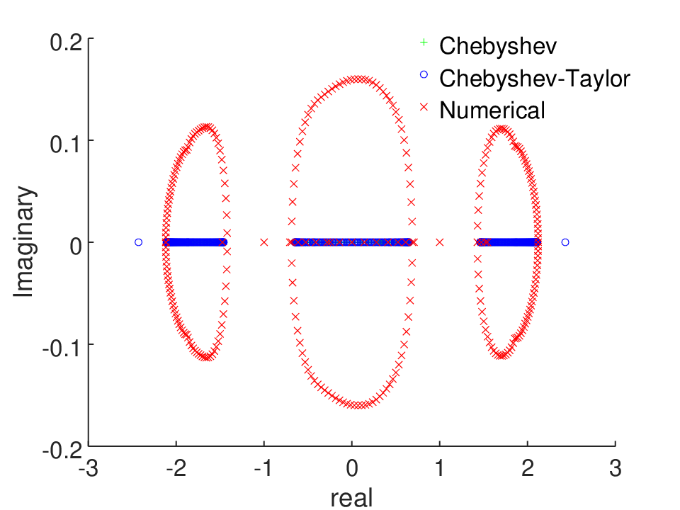
where coefficient is a degree polynomial and . This recurrence is of general interest, with widely used special cases such as the Chebyshev polynomials where , and . In the first section, we establish relations for the limiting set of roots of polynomials as , and other useful approximations of these roots for finite . Limiting roots of polynomials generated by a general three-term recurrence was recently studied by other approaches [1] where the effect of initial conditions and had to be analyzed separately. Limiting behaviour of such general three term recurrences with analytic functions as coefficients [2] and general higher order recurrences [3] have also been examined with applications in approximation theory. Similarly, specific cases of the above given polynomial recurrence with real coefficients and a particular value of were also studied [4, 5]. Our analysis of the polynomial recurrence of interest in the first part of this paper includes the effect of initial conditions, the different rates of convergence to the limiting set, approximations for finite and their errors. These approximations are motivated by both large errors and the large computational efforts required in iterative numerical methods applied to eigenvalue problems or the corresponding root-finding problems. Large errors due to the accumulation of digital round-offs are common when some roots are close to zero, as often is the case when modeling natural and man-made systems (see Figure 1 for an example). In the second part of the paper, we first show the significance of these results for eigenvalue problems that represent any chain of periodicity . Note that roots of these polynomials can also represent eigenvalues of tridiagonal matrices with -periodicity in their entries. A few examples are presented as a demonstration of the theorems. Later, we use Kronecker products and sums to extend this semi-analytical approach to matrices representing periodic graphs that need not be banded or of Toeplitz kind.
1 Existence of a limiting set and the nature of convergence of roots
Let be the set of points in the complex plane such that for any , for any , there exists an such that for all there is always at least one root of in the -neighbourhood of . We call the maximal such as the limiting set (i.e. no other set containing satisfies this property). There can be other notions of a limiting set [6]. To show that roots of the polynomials defined in three term recurrence (1) have a limiting set as , it is sufficient to show that there exists a corresponding eigenvalue problem with a limiting distribution. In the context of this work, we show that for roots of the polynomial we have a related eigenvalue problem. This would allow us to study its convergence to a limiting set and apply it effectively for approximations in the case of finite . The polynomials are of degree and can be expanded as determinant of the following matrix
| (2) |
Without loss of generality we consider , as can be normalized correspondingly for the determinant to satisfy the recurrence for other values of . Here the constant is non-zero, else the three term recurrence becomes trivial. Also note that both signs of the square roots in equation (2) results in the same three term recurrence.
Let . By factoring out , the roots of can be reformulated as the solutions of . Here is an eigenvalue of the matrix
| (3) |
Let be the characteristic polynomial for the above matrix and be the characteristic polynomial for a skew symmetric matrix
| (4) |
Then we have
| (5) |
The recurrence relation for the characteristic polynomials of is given by
| (6) |
From equations (5) and (6), we also have
| (7) |
For the matrix , let be the eigenvalues and hence . Since , we also know . Let the matrix in equation (7) have a determinant , and by using its diagonal decomposition we rewrite it as11 1 Note that is uniquely determined by and continuously varies with the two roots , and the branch cuts of square roots do not affect the results of this analysis.
| (8) |
Since , when we have
| (9) |
This gives us the following relations for zeros of that solve the required eigenvalue problem in equation (3):
| (10) | ||||
| (11) |
By considering equation (11) as a polynomial in , the absolute value of product of all zeros is one. By applying Landau’s inequality 22 2 Absolute value of, the product of all zeros with magnitudes greater than one, is at most ., product of the zeros with absolute values greater than one is at most . Note that is bounded in the region of interest. So as increases the absolute value of zeros approaches one, and so does the fraction of such zeros. This establishes the existence of a limiting spectrum for .
Convergence to the limiting set
The convergence of zeros of can be obtained using Rouche’s theorem. If for any , we are able to find an such that
then there are exactly zeros of the polynomial which have magnitude less than . Let us denote by . In equation (11) as a polynomial in , we are concerned with the polynomial . So for a value of , let
| (12) |
Now by dividing the equation above by we get
| (13) |
This implies if is the upper bound for magnitude of zeros of , then from equation (13) is the lower bound for the magnitude of all its zeros. Similarly if is the upper bound for magnitude of zeros, then is an upper bound for magnitude of one zero. We divide the analysis into , and , and consider these three cases separately.
- 1.
(14) (15) (16) Note that and . Also, for some . Forcing the lower bound of the left side of the equation to be greater than the upper bound on the right hand side in equation ((16)), we get a lower bound on as follows :
(17) (18) (19) (20) This implies for some , this upper bound for magnitude of all zeros given by asymptotically approaches one. From the previous arguments is a lower bound for magnitude of all zeros, and this asymptotically approaches one as well.
- 2.
When , we assume is the upper bound for magnitude of zeros, and derive a lower bound for in the following manner, starting with equation (15) again :
(21) (22) (23) (24) Thus an upper bound for magnitude of all the zeros is with any , and lower bound for the magnitudes is , and these asymptotically approach one as well.
- 3.
When , consider
We again find a such that satisfies the above, which is equivalent to
(25) Note that and also for some . Forcing the lower bound of the left side of the equation to be greater than the upper bound on the right hand side in equation (3), we get a lower bound on as follows:
(26) Since is a sufficient lower bound for in the case of large ,
(27) (28) (29) (30) is the upperbound for magnitude of zeros, and is an upper bound for magnitude of one zero. This implies except two zeros, all other zeros asymptotically converge to one. Consider (11) which can be rearranged to
(31) For let us denote as , and equation (31) can be read as
(32) Similarly, for let us denote as and rewrite equation (31) as
(33) As , we have , for and respectively, resulting in two limiting zeros and as well for the case-3 where .33 3 Alternately, by applying Landau’s inequality again on (11) after a change of variable from it can be shown that there is a zero approaching with the rate . These two zeros of also provide a condition for the limiting roots of the polynomials in recurrence; in addition to all the other limiting zeros of that converge to the unit circle as shown before.
From the above three cases we have the limiting zeros of given by unit circle . Given , we get the condition for the limiting set, which corresponds to continuous curves. But in case of , we have two zeros of that do not converge to the unit circle. These two zeros provide the same additional eigenvalue problem . Here is a polynomial of degree at most given by . This solution represents up to a maximum of points that may lie outside the continuous curves.
Theorem 1.
The limiting roots of polynomials in the three-term recurrence relation with , is a subset of , where .
The proof is from the previous analysis.
We denote the set and the set , so that contains the limiting set. The set is continuous and can be viewed as the curve in three dimension (), with real and imaginary part of being axis and being the axis (see section 2.3 for graphic examples).
Corollary 1.
For the continuous set , we have following three cases when is real.
- 1.
When is purely real and positive, then ; and line is a purely imaginary interval .
- 2.
When , the spectrum reduces to distinct points independent of dimension .
- 3.
When is purely real and negative, then and is a purely real interval .
Corollary 2.
The limiting roots of the polynomials in a three-term recurrence of the form with , in , are dense on the continuous set .
For the rigorous proof of this statement we refer the reader to another work [1] which makes use of Ismail’s -Discriminants along with theorems from other works [7]. Here, using equation (5) i.e. , we provide a reasonable argument for the above. Let for be the roots of and be the roots of . We know as . Thus for all we have from equation (5), as ,
| (34) |
Note that the roots of are dense on its support in its limiting case, and so the zeros of have to be dense as well.
1.1 Finite- approximations
Equation (34) justifies approximating zeros of by the roots of for finite large . As the roots of are distributed on the imaginary line just as the real roots of Chebyshev polynomials of second kind, we call this a Chebyshev approximation. The roots are the solution of in the following equation, where with are the roots of :
| (35) |
With the limiting behavior of zeros in equation (34), one can also further expand the relation , by a Taylor series approximation which is denoted as Chebyshev-Taylor approximation in this work. Let and be the roots of and respectively that are closest to each other. Given , the zero of can be approximated using a first order Taylor approximation as the following:
| (36) | ||||
| (37) |
With and being nearby roots, we consider . We can also see from the previous analysis that for sufficiently large ,
| (38) |
Here we have a front factor of in bounding values of using the convergence of to the unit circle in the previous section. So the roots of are approximated by solving for in the equation
| (39) |
For Chebyshev-Taylor approximation of eigenvalues, we first compute the solutions of using equation (35) and a . We then use roots of , and evaluated to improve this Chebyshev approximation of a root by solving equation (39) for . We finally identify the solution closest to among the solutions of , as the improved approximation. This approach, in principle, can be further extended into an iterative procedure or an higher-order approximation if required.

2 Evaluating spectra of chains and periodic graphs
The analyzed three-term recurrence is also satisfied by characteristic polynomials of tridiagonal matrices with -periodic entries on the three diagonals, and of corresponding dimensions . Here initial condition for the recurrence is not independent of the polynomial , as both arise from entries of the first rows of the matrix (see equations (43) and (51)). If is the natural number representing periodicity of entries, such matrices can be called tridiagonal -Toeplitz matrices. Roots of these characteristic polynomials represent the behavior of man-made and natural systems which contain a large number of units arranged periodically. Periodicity in natural and man-made systems have been of great interest and resulted in corresponding theories of Bloch, Hill, Floquet, Lyapunov and others. For example, Bloch’s theory of sinusoidal waves in a simple periodic potential (=1, ) has been widely applied; here real-valued spectra representing basis waves of the system results from a periodic phase-condition applied on the set of all possible waves. In this work, with variables in and imaginary entries that need not result in a Hermitian, we allow for both dissipative and generative properties in the chain and thus conditions on both phase and amplitude define the limiting complex roots.
Many problems in physics, economics, biology and engineering are modelled using chains and spatial lattices, and the more general case is a graph that has a periodic structure. In a chain each repeated unit can in-turn be composite, and thus contain interconnected elements or elements of multiple types resulting in a periodicity . There are classical chain models like Ising model, the structural model for graphene [8] and worm like chains in microbiology [9]. Such chain models can be reduced to a system of equations represented by a tridiagonal matrix [10],[4],[11] with periodic entries. The tridiagonal matrix of interest is Hermitian with real spectra in cases like some spring-mass systems, electrical ladder networks and Markov chains. It can be non-Hermitian in the case of other chain models in economics and physical systems that break certain reflection symmetries, behave non-locally, or do not entail conservation of energy [12], [13]. Limiting cases of tridiagonal -Toeplitz and -Toeplitz matrices with only real entries were studied [5], and so were tridiagonal -Toepltiz matrices similar to a real symmetric matrix [4], all of which produce the above three-term polynomial recurrence for , in . In case of tridiagonal -Toeplitz matrices, we also show in the appendix that the continuous part of the limiting set of roots can alternately be derived using Widom’s conditional theorems for existence of limiting spectra of block-Toeplitz operators [14], [15] and its recent extensions [16]. Whereas, the analysis in previous sections also included nature of convergence and the up-to critical roots that depend on initial conditions of the recurrence, which may not converge to this continuous set; evaluation of these critical roots are significant in chain and lattice models.
A chain with periodicity is especially useful in modeling periodic graphs such as a spatial lattice of higher dimensions. Although the existence of a limiting set of roots even for a recurrence with more than three terms is known[17], it is not clear if periodic graphs submit to such recurrence relations. Alternately, we can apply the spectral rules of tensor products along with the spectra of such composite chains, to evaluate spectra of many spatial lattices and periodic graphs even when the unit cells are heterogeneous. This is shown in Section 2.4.
In the next section 2.1, characteristic polynomials of tridiagonal -Toeplitz matrices are shown to satisfy the recurrence of interest. This is followed by a section on some chain models and special -Toeplitz matrices , which serves as an example for important such recurrence relations with variables in . Finally, a few numerical examples are used in section 2.3 to demonstrate the utility of theorems and the generalized spectral relations of chains for variables in . We begin with characteristic polynomials of tridiagonal -Toeplitz matrices; here tridiagonal elements repeat after rows. They are of the form
Here we have the periodicity constraints , and , and , and are complex numbers.
2.1 Three term recurrence of polynomials from a general tridiagonal -Toeplitz matrix
Our objective in this section is to show a three-term recurrence relation of characteristic polynomial of matrix of dimension , in terms of characteristic polynomials of matrices of dimensions and . We do this by expanding the determinant.
Characteristic equation of matrix is given by the polynomial and let , then
Let denote the characteristic polynomial of matrix of dimension () and be the characteristic polynomial of the first principal sub-matrix of eliminating first row and first column, which is of dimension . Similarly let be the characteristic polynomial of the second principal sub-matrix obtained by eliminating first two rows and first two columns, and . Then we have
| (40) |
In the matrix form of the above, we have
| (41) |
This gives us
| (42) |
with the initial condition
| (43) |
Note that when , and will reduce to and without any loss of generality of the above. Similarly will reduce to in the case of . Let us denote . Also let . Entries of are polynomials in , and for generality let us denote them as , where and are some polynomials of degree at most . Therefore
| (44) |
Proposition 1.
The characteristic polynomial of a tridiagonal k-Toeplitz matrix satisfies the following recurrence relation, where k is the period and nk is the dimension of the matrix:
| (45) |
Here is a polynomial of degree k, and .
Proof.
From equation (44) we have
| (46) | ||||
| (47) |
Rearranging equation (46) and replacing by , we have
| (48) |
Multiplying (47) by we have
| (49) |
This can be further reduced using matrices as
| (50) | ||||
| (51) |
We have and .
This proves the proposition with and .
∎
Corollary 3.
From proposition-1, we have the three term recurrence in the matrix form
| (52) |
Let . The eigenvalues of are
| (53) |
with the corresponding eigenvectors
By relationship of the determinant to eigenvalues, we also have for all .
Corollary 4.
Suppose two tridiagonal -Toeplitz matrices with entries and with entries have the relation and then this is a sufficient condition for both of them to have an identical limiting spectrum. In case of , this is the necessary and sufficient condition.
2.2 A chain with complex spectra :
In this section, we apply our results to characteristic polynomials of tridiagonal -Toeplitz matrices that represent a chain where Hermitian blocks (representing non-dissipative units) are joined by non-Hermitian blocks (representing a source-sink pair). Such chains exhibit unique modes that span dissipative, transitive and generative properties. We define tridiagonal -Toeplitz matrices , where and . Here is any odd number or 2. If is any even number other than 2, spectra of is identical to that of of corresponding dimensions.
Examples:


For with , where be the dimension of matrix, eigenvalues are plotted in figure 3. The corresponding values of are and . We discuss cases with without loss of generality as any other constant just induces a shift in the spectra by the value . The following observations on spectra of are later derived using Theorem 1 stated in the first part of this paper.
2.2.1 Observations and claims on
- 1.
All for a fixed have same limiting spectrum. Note that this property follows as and depend only on the product of the off-diagonal entries.
- 2.
Spectrum of (plotted real versus imaginary part of eigenvalues of large dimension ) for converges to distinct curves. This is established by Theorem 2.
- 3.
Let be of the form where is a natural number. One of the curves traced by eigenvalues is along the imaginary axis if is even, and the eigenvalues trace a line on the real axis if is odd. This follows from Theorem 2 as well.
Here dimension of the matrix is considered as an integer multiple of . If it is not, then number of eigenvalues may lie outside the curves traced in complex plane. Note that a general requirement of symmetry in eigenvalues exists for matrices with alternating zero and non-zero sub-diagonals; see Remark 1 in the appendix.
2.2.2 Limiting spectra of
In this section we use the procedure described in section 2.1 to explicitly derive and in the three-term recurrence relations of characteristic polynomials of matrices . This allows us to prove the properties of limiting spectra of matrices claimed in section 2.2.1 by applying the theorems in section 1. As mentioned before, spectrum of for an even number reduces to that of and hence is not discussed further. Let the odd natural number where . Let when is odd and when is even.
Theorem 2.
Characteristic polynomial of any of dimension satisfies the three-term recurrence relation given by
| (54) |
where
| (55) |
when is odd, and
| (56) |
when is even.
The proof of the above theorem is provided in the appendix.
2.3 Numerical examples of chains
In this section we present a few example solutions of eigenvalues, both in the case of a matrix and other general tridiagonal -Toeplitz matrices . The polynomial has distinct roots for any point in . These roots can be well approximated using Chebyshev roots on line which become dense in the limiting case (section 1.1). As pointed before, such evaluations cost arithmetic operations while numerical evaluations cost . In many applications where is large, tracing these curves as the support for eigenvalues using fewer points on may be sufficient. As the points on vary smoothly, these roots can be viewed as curves in three dimensional space (X, Y axis representing real and imaginary parts of , and Z axis corresponding to ). Therefore limiting eigenvalues are supported by the curve in space.
2.3.1
- 1.
For a graphic example of , we have with . For , we have , with . For we have with . These curves, their projections and eigenvalues for a large can be seen in figure 4.
- 2.
Note that when is of the form , spectrum contains real axis as one of the curve and of the form spectrum contains imaginary axis as one of the curves (Theorem 2).
- 3.
Convergence of the absolute value of eigenvalues of recurrence matrix i.e. defined in section 2.1, indicates the convergence to the limiting spectrum for tridiagonal -Toeplitz matrices (as shown in appendix using Widom’s theorems). In figure 5, the maximum, minimum and average of absolute are plotted for with .


2.3.2
In , when we can limit our discussion to matrices of the form
Here and spectrum of the matrix is shifted from that of by a value . In this section we consider and when we apply Proposition 1 we get expressions for and for these examples. Let ; then
| (57) | ||||
| (58) |
As an example, and were taken from uniform disc of radius 1 in the complex plane and Theorem 1 was applied to generate limiting supports for the eigenvalue distribution. Matrices of dimension 500 are shown in Figures 7 and 7.


2.4 Spectra of graphs generated by Kronecker sums and products of chains
A graph having the vertex set and edges connecting those vertices with weight is represented as . Let and be two graphs with same number of vertices, having weights and with weight being zero if there is no edge between corresponding pair of vertices. The Kronecker sum is a graph with the vertex set with with and . There is an edge between and if ans or and .
Let the matrices and be the adjacency matrices of and respectively, then the adjacency matrix of is given by
Here when and zero otherwise. The adjacency matrix can also be written as a Kronecker sum which is
| (59) |
where is a Kronecker product. The Laplacian, (defined as where ) of the graph is also the Kronecker sum of the individual Laplacians. If and are the Laplacians of graph and , then
| (60) |
By similar arguments, the Cartesian sum of the three graphs , and have the adjacency matrix , which is
| (61) | ||||
| (62) |
Similarly the Laplacian is given as
| (63) |
When the individual graphs are chains, we get a square lattice as a Kronecker sum of two chains. The resulting Laplacian is also the Kronecker sum of the Laplacian of the two individual chains. Suppose and be the Laplacians of two and periodic chains having and type of distinct elements. Then is the Laplacian of a periodic square lattice having rectangular patch periodically repeating in and directions. Consider the Laplacian of the graph , which is
Let and be the eigenvalues and eigenvector relations satisfied by and , then we have
| (64) | ||||
| (65) |
The eigenvalues of the resulting Laplacian are all the possible sums of pairs of the eigenvalues of the individual Laplacians. Similarly, for the Kronecker sum of three graphs, resulting eigenvalues are all possible sums of the eigenvalues of the three Laplacians. Hence error in the approximated eigenvalues is the sum of the individual errors. Figure 8 shows the spectrum of a spatial lattice constituted with two different periodic chains of period two, sketched in figure 9. A periodic graph can also be constructed by simple Kronecker products of two chains (shown in figure 11), which results in all the possible products of pairs of eigenvalues in figure 10.


3 Summary
We analyzed the behavior of roots of polynomials with a three-term recurrence relation of the form , where the coefficient is any degree polynomial, and . In addition to establishing existence and convergence to a limiting set of roots for generality of variables in and any , useful approximations for roots in case of finite were derived. A slower convergence to the limiting set of roots by an order of was shown to be possible for some cases, compared to the expected order of . Relations for the up-to critical roots which depend on the initial conditions and lie outside the continuous limiting set, were also derived. These results were applied to eigenvalue problems of tridiagonal -Toeplitz matrices which represent models of chains with different elements. Note that spectra of such chains allow one to efficiently and accurately evaluate spectra of many heterogeneous spatial lattices and other periodic graphs as well, using spectral rules of Kronecker products. Numerical examples were used as a demonstration of theorems later. These closed-form solutions and approximations can substitute iterative numerical methods for solution of these eigenvalue problems, as the latter involve significantly larger computational effort and are error prone.
Appendix
Proof of Theorem 2 :
Let the odd natural number . Let when is odd and when is even.
Proof.
For the matrices we have for . Also . For and we have, . Therefore we obtain, and .
These relations can also be written as
| (66) | ||||
| (67) |
Corresponding initial matrices with and are
For equation (67), initial conditions are
With these two initial conditions and recurrence relation (67) we obtain coefficients of where
| Value of | m | |||||||
| 0 | 0 | 0 | 0 | 0 | 0 | 1 | 1 | 1 |
| 0 | 0 | 0 | 0 | 0 | 1 | -1 | 3 | 2 |
| 0 | 0 | 0 | 0 | 1 | -1 | 1 | 5 | 3 |
| 0 | 0 | 0 | 1 | -1 | 2 | -1 | 7 | 4 |
| 0 | 0 | 1 | -1 | 3 | -2 | 1 | 9 | 5 |
| 0 | 1 | -1 | 4 | -3 | 3 | -1 | 11 | 6 |
| 1 | -1 | 5 | -4 | 6 | -3 | 1 | 13 | 7 |
Table 1 shows values corresponding to first few . Let be an element at row column in table 1. Where and start from top right corner. Here corresponding to . From equation (67) we have
| (69) |
with appropriate initial conditions.
The table 1 can be seen as two pascal triangles one with initial condition 1 and another with initial condition -1. is the entry in the row and the column of the pascal triangle and that will be . Similarly is given by entries in row and column of another pascal triangle and this is . Using the above, we construct the polynomial as
| (70) |
when is odd, and
| (71) |
when is even. ∎
The limiting set C and conditional theorems based on Toeplitz operators
In the special case of characteristic polynomials of tridiagonal matrices and the recurrence relation of interest here, the continuous limiting set C can be as well derived from more general theorems for existence of the limiting spectrum for block-Toeplitz matrices and banded Toepltiz matrices. In the case of block-Toepltiz operators, the limiting spectra were shown to exist under certain conditions by H. Widom [14] and [15]. Extension of this theory to the equilibrium problem for an arbitrary algebraic curve was presented in a recent article [16], and in this brief note, we maintain the notations used there. Here we treat the tridiagonal -Toeplitz matrix as a block-Toeplitz matrix. The for the matrix was defined as
| (72) |
Here,
The spectrum is determined by an algebraic curve and in this case it is a quadratic polynomial. The limiting spectrum of the tridiagonal block-Toeplitz matrix is given by all where both roots of the quadratic polynomial have same magnitude [14]. This is valid under certain assumptions (named H1,H2, H3) as shown by Delvaux [16]. Let the quadratic polynomial be of the form . Below we show that and are identical, also showing that the relevant theorems of Widom and Delvaux can be reduced to derive the continuous set in the limiting spectra of tridiagonal -Toeplitz matrices. The coefficients have to be evaluated by finding the determinant. To do this, consider a permutation matrix
and and . By applying the expansion for determinant of such matrices (provided in [18]) to we get
with,
Let be the roots of quadratic equation . In the case of limiting large it was shown by those authors that the quadratic polynomial has two roots of equal magnitude. So this gives a corresponding condition . So the coefficient is related to the determinant as
| (73) |
With a change of notation from to , by rewriting and we get
| (74) |
The above defines the continuous set and implies the same condition on as in Theorem 1.
Similarly in [2], the authors consider a three term recurrence of a general form which is,
Here is related to the determinant of the matrix,
The entries are analytic in a domain and they are asymptotically periodic. If denote the matrix with first rows and columns removed, . The corresponding matrix can be called as almost -Toeplitz matrix. The related chains can be termed as almost -periodic chains. In [2] authors establish the asymptotic ratio of and as an analytic function in certain domain, using properties of continued fractions. Thus it establishes the theoretical basis for the analysis of limiting and finite- spectra for the almost -Toeplitz matrices.
Symmetry in spectrum of odd diagonal matrices
Let the diagonals of a square matrix be indexed such that the main diagonal is zeroth diagonal, and diagonals above and below it are numbered sequentially using positive and negative integers respectively. Then, odd-diagonal matrices refer to matrices with non-zero entries only on the odd-numbered diagonals. In this section we show that a significant reflection symmetry exists in the spectra of all odd diagonal matrices with constant entries on the main diagonal, including -Toeplitz matrices of this kind.
Remark 1.
- 1.
Suppose two square matrices commute up to a constant , i.e. and is non-singular, then if is eigenvalue of with eigenvector , then is also an eigenvalue with a corresponding eigenvector .
Proof.
From the statement of the theorem,
∎
- 2.
For a square matrix with zeros on the even indexed diagonals, and a square matrix with as entries in the diagonal and all other entries as zeros, the above result applies with . Therefore eigenvalues of and occur in pairs, when the main diagonal consists of constant entries .
References
- [1] K. Tran, The root distribution of polynomials with a three-term recurrence, J. Math. Anal. Appl. 421 (2015) 878–892.
- [2] D. B. Rolania, G. L. Lagomasino, Asymptotic behavior of solutions of general three term recurrence relations, Adv. Comp. Math. 26 (1-3) (2007) 9–37.
- [3] D. B. Rolanía, J. S. Geronimo, G. L. Lagomasino, High-order recurrence relations, Hermite-Padé approximation and Nikishin systems, Sbornik: Mathematics 209 (3) (2018) 385.
- [4] R. Álvarez-Nodarse, J. Petronilho, N. Quintero, Spectral properties of certain tridiagonal matrices, Linear Algebra Appl. 436 (3) (2012) 682–698.
- [5] F. Marcellán, J. Petronilho, Eigenproblems for tridiagonal 2-Toeplitz matrices and quadratic polynomial mappings, Linear Algebra Appl. 260 (1997) 169–208.
- [6] P. Schmidt, F. Spitzer, The Toeplitz matrices of an arbitrary Laurent polynomial, Math. Scand. 8 (1) (1960) 15–38.
- [7] A. D. Sokal, Chromatic roots are dense in the whole complex plane, Comb. Probab. Comput. 13 (2004) 221–261.
- [8] A. Matulis, F. Peeters, Analogy between one-dimensional chain models and graphene, Amer. J. Phys. 77 (7) (2009) 595–601.
- [9] C. Storm, J. J. Pastore, F. C. MacKintosh, T. C. Lubensky, P. A. Janmey, Nonlinear elasticity in biological gels, Nature 435 (7039) (2005) 191–194.
- [10] A. Šiber, Dynamics and (de) localization in a one-dimensional tight-binding chain, Amer. J. Phys. 74 (8) (2006) 692–698.
- [11] K. Parthasarathy, R. Sengupta, Exchangeable, stationary, and entangled chains of Gaussian states, J. Math. Physics 56 (10) (2015) 102203.
- [12] M. Znojil, Tridiagonal-symmetric N-by-N Hamiltonians and a fine-tuning of their observability domains in the strongly non-Hermitian regime, J. Phys. A 40 (43) (2007) 13131.
- [13] C. M. Bender, Making sense of non-Hermitian Hamiltonians, Rep. Prog. Phys. 70 (6) (2007) 947.
- [14] H. Widom, Asymptotic behavior of block Toeplitz matrices and determinants, Adv. Math. 13 (3) (1974) 284–322.
- [15] H. Widom, Asymptotic behavior of block Toeplitz matrices and determinants ii, Adv. Math. 21 (1) (1976) 1–29.
- [16] S. Delvaux, Equilibrium problem for the eigenvalues of banded block Toeplitz matrices, Math. Nachr. 285 (16) (2012) 1935–1962.
- [17] S. Beraha, J. Kahane, N. J. Weiss, Limits of zeroes of recursively defined polynomials, Proc. Natl. Acad. Sci. 72 (11) (1975) 4209.
- [18] L. G. Molinari, Determinants of block tridiagonal matrices, Linear Algebra Appl. 429 (8) (2008) 2221–2226.