跳到论文正文
W Papers独立论文阅读器 arXiv:1506.05301 论文正文 计算阅读时间 · 0%
引用这篇论文根据当前论文元数据生成,正式投稿前建议核对。


License: arXiv.org perpetual non-exclusive license
arXiv:1506.05301v1 [hep-ph] 17 Jun 2015

PSI-PR-15-06

ZU-TH 14/15

August 24, 2026

SCET approach to regularization-scheme dependence of QCD amplitudes

A. Broggioa, Ch. Gnendigerb, A. Signera,c, D. Stöckingerb, A. Viscontia,c
a Paul Scherrer Institut,
CH-5232 Villigen PSI, Switzerland

b Institut für Kern- und Teilchenphysik,
TU Dresden, D-01062 Dresden, Germany

c Physik-Institut, Universität Zürich,
Winterthurerstrasse 190, CH-8057 Zürich, Switzerland

PACS numbers: 11.10.Gh, 11.15.-q, 12.38.Bx


Abstract

We investigate the regularization-scheme dependence of scattering amplitudes in massless QCD and find that the four-dimensional helicity scheme (FDH) and dimensional reduction (DRED) are consistent at least up to NNLO in the perturbative expansion if renormalization is done appropriately. Scheme dependence is shown to be deeply linked to the structure of UV and IR singularities. We use jet and soft functions defined in soft-collinear effective theory (SCET) to efficiently extract the relevant anomalous dimensions in the different schemes. This result allows us to construct transition rules for scattering amplitudes between different schemes (CDR, HV, FDH, DRED) up to NNLO in massless QCD. We also show by explicit calculation that the hard, soft and jet functions in SCET are regularization-scheme independent.

1 Introduction

Higher-order calculations in QCD result in loop integrals that are often ultraviolet (UV) and/or infrared (IR) divergent. The standard method to deal with these singularities is dimensional regularization, where space-time is shifted from 4 to D≡4−2​ϵD\equiv 4-2\epsilon dimensions. The UV and IR singularities then manifest themselves as poles 1/ϵk1/\epsilon^{k}.

There are several variants of dimensional regularization. The most common scheme is conventional dimensional regularization (cdr), where all vector bosons are treated as DD-dimensional. From a conceptual point of view this is the simplest possibility and guarantees a consistent treatment. However, cdr  has some disadvantages. Apart from breaking supersymmetry, it is also not directly compatible with the helicity method and other computational techniques that rely on 4 dimensions and, hence, leads to more tedious expressions in intermediate steps of a calculation. Therefore, it is often advantageous to use other schemes, such as the ’t Hooft-Veltman scheme (hv) [1], dimensional reduction (dred) [2] or the four-dimensional helicity scheme (fdh) [3].

The result for a physical quantity such as a cross section is of course finite and must not depend on the regularization scheme that has been used. However, in practise such a result is obtained as a sum of several contributions, which usually are separately divergent. Therefore, these partial results can depend on the regularization scheme. It is often advantageous to use regularization schemes that are adapted to the technique used for the computation of a particular contribution. In order to be able to consistently combine the various partial results it is then imperative to have full control over the scheme dependence.

The key observation is that the scheme dependence is actually intimately linked to the structure of UV and IR singularities. The singularity structure in fdh and dred is best understood if the (quasi) 4-dimensional gluons gg are split into DD-dimensional gluons g^{\hat{g}} and Nϵ=2​ϵN_{\epsilon}=2\epsilon scalars g~{\tilde{g}}. From a conceptual point of view these so-called ϵ\epsilon-scalars g~{\tilde{g}} can be treated as independent fields with an initially arbitrary multiplicity NϵN_{\epsilon}. The identification Nϵ=2​ϵN_{\epsilon}=2\epsilon is to be made only at the end of a calculation. The decomposition of gg into g^{\hat{g}} and g~{\tilde{g}} has to be made in dred as well as in fdh. This seems to be a disadvantage of these schemes. However, it is useful to gain insight and to derive the scheme dependence, and for practical purposes, such an explicit separation is often not required.

The contributions of the ϵ\epsilon-scalars are UV and IR divergent, resulting in terms of the form (Nϵ)i/ϵk(N_{\epsilon})^{i}/\epsilon^{k}. It is precisely these terms that – after setting Nϵ=2​ϵN_{\epsilon}=2\epsilon – induce the scheme dependence in partial results. For a physical cross section the poles in ϵ\epsilon have to cancel, including poles of the form Nϵ/ϵN_{\epsilon}/\epsilon. This entails that the scheme dependence for a (finite) physical result can be at most 𝒪⁡(Nϵ​ϵ0){\cal O}(N_{\epsilon}\,\epsilon^{0}) and, hence, will vanish in the limit ϵ→0\epsilon\to 0. At next-to-leading order (NLO) this has been explicitly demonstrated [4]. However, virtual corrections generally are UV and IR divergent and, therefore, scheme dependent. To find this scheme dependence the structure of UV and IR singularities has to be understood for a gauge theory with gluons and ϵ\epsilon-scalars.

Regarding the UV singularities, the main point is that treating the ϵ\epsilon-scalars as independent fields induces additional couplings. The independence of these couplings and their UV renormalization was already required in the equivalence proof of dred  and cdr [5, 6, 7] and in explicit multi-loop calculations in dred [8, 9, 10]. It has to be stressed that also in fdh the couplings have to be treated as independent [4, 11].

The development regarding the scheme dependence related to the IR divergent part beyond NLO is more recent. The structure of the IR singularities for massless gauge amplitudes has a remarkably simple form [12, 13, 14, 15]. It can be expressed in terms of the cusp anomalous dimension γcusp\gamma_{\text{cusp}} and the anomalous dimensions of the quark and gluon, γq\gamma_{q} and γg\gamma_{g}, respectively. These anomalous dimensions have been extracted from explicit results of form factors computed in cdr and are consistent with other processes.

It seems natural to assume that this structure can be extended to other schemes by applying the split of gg into g^{\hat{g}} and g~{\tilde{g}}. This results in modified (i.e. scheme dependent) anomalous dimensions. At NLO, this leads to results that are consistent with the well-known scheme dependence of NLO amplitudes [16]. Based on this assumption, γcusp\gamma_{\text{cusp}}, γq\gamma_{q} and γg\gamma_{g} have been extracted in the fdh scheme at NNLO [17, 18], by comparing the generalized IR structure to explicit results of two-loop amplitudes for the γ∗→q​q¯\gamma^{*}\to q\bar{q} and H→g​gH\to gg form factors and the process q​q¯→g​γq\bar{q}\to g\gamma. Considering all these processes together yields an over-constrained system for the extraction of γcusp\gamma_{\text{cusp}}, γq\gamma_{q} and γg\gamma_{g} in the fdh scheme. The fact that there is a solution to this system suggests that fdh is a well defined scheme beyond NLO.

The main results of this paper are the following: First, we will provide further evidence that with a proper definition fdh can be used for loop calculations beyond NLO. To this end we show that the anomalous dimensions γcusp\gamma_{\text{cusp}}, γq\gamma_{q} and γg\gamma_{g} can be computed directly in soft-collinear effective theory (SCET) [19, 20, 21, 22, 23, 24, 25, 26, 27] by relating them to the jet- and soft functions. We repeat the original calculation of the quark-jet function [28] and gluon-jet function [29] in the fdh scheme and also determine the soft function in fdh. This gives us an independent determination of γcusp\gamma_{\text{cusp}}, γq\gamma_{q} and γg\gamma_{g} in the fdh scheme and the results we find are in agreement with previous findings. Note that the fdh as we use it [4, 17] is slightly different from previous implementations [30].

Second, we extend the scheme dependence study to dred. While the anomalous dimensions in dred are the same as in fdh we also need to consider amplitudes with external ϵ\epsilon-scalars. Determination of the IR structure of these amplitudes requires the knowledge of γϵ\gamma_{\epsilon}, the anomalous dimension of the ϵ\epsilon-scalar g~{\tilde{g}}. We compute γϵ\gamma_{\epsilon} in SCET via the calculation of the g~{\tilde{g}}-jet and soft functions and give the generalization of the IR structure to amplitudes with external g~{\tilde{g}}. Furthermore, we verify that this result for γϵ\gamma_{\epsilon} is in agreement with the result extracted from an explicit computation of H→g~​g~H\to{\tilde{g}}{\tilde{g}} at NNLO [31]. We thus obtain a complete understanding of the relations between NNLO amplitudes with gluons and massless quarks computed in cdr, hv, fdh, and dred.

Finally, we gain insights into how the regularization-scheme dependence cancels for fully differential cross sections at NNLO. While a complete study of this issue is beyond the scope of this work, our calculations in SCET show that the jet- and soft functions are separately scheme independent. The same is true for the hard function. Hence, if the cross section is written as a convolution of hard-, soft-, and jet functions it is manifestly regularization-scheme independent. Recently there has been a lot of activity in performing fully differential NNLO calculations using the SCET framework. This development started with the computation of top-quark decay [32] and has then been extended to more generic cases [33, 34, 35]. The results of our work show how to apply a particular regularization scheme for the calculation of either the hard-, soft- or jet function. For each of these building blocks separately, the most convenient regularization scheme can be used. This opens up possibilities for further technical advances.

The paper is organized as follows: In Section 2 we briefly review the various regularization schemes and discuss how they affect the IR structure of scattering amplitudes. Section 3 is devoted to the computation of the anomalous dimensions that are required for the IR structure. These computations are done in SCET. An alternative determination of the anomalous dimension of the ϵ\epsilon-scalar is presented in Section 4, where we extract γϵ\gamma_{\epsilon} from the gluon form factor computed in dred. In Section 5 we use these results to obtain explicit transition rules for two-loop amplitudes between hv and fdh, as well as between fdh and dred. The transition rules are then checked with explicit examples. Our conclusions including a discussion on the scheme independence of cross sections at NNLO are presented in Section 6. Finally, we give some explicit results of the SCET computations in Appendix A and list the required anomalous dimensions and β\beta functions in all schemes in Appendix B.

2 Schemes and structure of IR singularities

2.1 Regularization schemes

Dimensional reduction has been shown to be mathematically consistent [36] and equivalent to dimensional regularization [7, 6] on the level of IR finite Green functions. In the way we define it, the fdh scheme has the same properties. The consistent implementation of the considered regularization schemes requires the introduction of three vector spaces. Apart from the strictly 4-dimensional space (4S) with metric g¯μ​ν{\bar{g}}^{\mu\nu} two infinite-dimensional spaces have to be introduced, the quasi 4-dimensional space Q4S [37, 38, 36] with metric gμ​νg^{\mu\nu} satisfying gμμ=4g^{\mu}_{\ \mu}=4 and quasi DD-dimensional space QDDS with metric g^μ​ν{\hat{g}}^{\mu\nu} satisfying g^μμ=D{\hat{g}}^{\mu}_{\ \mu}=D. The structure Q4S ⊃\supset QDDS ⊃\supset 4S is reflected in the properties of the various metric tensors: gμ​ν​g^ν​ρ=g^ρμg^{\mu\nu}{\hat{g}}_{\nu\rho}={\hat{g}}^{\mu}_{\ \rho} and g^μ​ν​g¯ν​ρ=g¯ρμ{\hat{g}}^{\mu\nu}{\bar{g}}_{\nu\rho}={\bar{g}}^{\mu}_{\ \rho}.

For a detailed discussion and a precise definition of the four considered regularization schemes (rs) we refer to Ref [4]. Here we only repeat the most important aspects to facilitate the following discussion. The various rs differ in the way “internal gluons” (part of a one-particle irreducible loop diagram or unresolved final state gluon) and “external gluons” (all remaining gluons) are treated. This is summarized in Table 1 taken from Ref. [4]. Since external gluons are treated as stricly 4-dimensional in fdh and hv these schemes are best adapted to be used in connection with the helicity method.

cdr hv dred fdh
internal gluon g^μ​ν{\hat{g}}^{\mu\nu} g^μ​ν{\hat{g}}^{\mu\nu} gμ​νg^{\mu\nu} gμ​νg^{\mu\nu}
external gluon g^μ​ν{\hat{g}}^{\mu\nu} g¯μ​ν{\bar{g}}^{\mu\nu} gμ​νg^{\mu\nu} g¯μ​ν{\bar{g}}^{\mu\nu}

Table 1: Treatment of internal and external gluons in the four different rs, i.e. prescription for which metric tensor is to be used in propagator numerators and polarization sums.

The cleanest way to understand the scheme differences is to consistently apply the split of the (quasi) 4-dimensional gluon into a DD-dimensional gluon and an ϵ\epsilon-scalar. This is done at the level of the Lagrangian writing the field of the 4-dimensional gluon field of fdh and dred as Aμ=A^μ+A~μA^{\mu}=\hat{A}^{\mu}+\tilde{A}^{\mu}, where A^μ\hat{A}^{\mu} and A~μ\tilde{A}^{\mu} are the DD-dimensional gauge field and the ϵ\epsilon-scalar field, respectively [5]. We will denote the associated ’particles’ as g^{\hat{g}} and g~{\tilde{g}}, respectively. The ϵ\epsilon-scalars have an initially independent multiplicity NϵN_{\epsilon} and the metric g~μ​ν{\tilde{g}}^{\mu\nu} associated with g~{\tilde{g}} satisfies the orthogonality relation g^μ​ν​g~ν​ρ=0{\hat{g}}^{\mu\nu}{\tilde{g}}_{\nu\rho}=0 and g~μ​ν​g~μ​ν=Nϵ{\tilde{g}}^{\mu\nu}{\tilde{g}}_{\mu\nu}=N_{\epsilon}. Scheme differences have their origin in UV and IR divergent contributions due to these ϵ\epsilon-scalars. These contributions are of the form (Nϵ)i/ϵk(N_{\epsilon})^{i}/\epsilon^{k} and after setting Nϵ→2​ϵN_{\epsilon}\to 2\epsilon result in the scheme differences. This connection to UV and IR singular terms allows for a completely systematic treatment of the rs dependence.

Regarding UV renormalization, fdh and dred behave in the same way. The possible split of internal gluons into gauge fields and ϵ\epsilon-scalars implies that in principle five different couplings need to be distinguished (see in particular [7, 8, 11]): the gauge coupling αs\alpha_{s}, the g~​q​q¯{\tilde{g}}q\bar{q} coupling αe\alpha_{e}, and three different independent quartic g~{\tilde{g}}-couplings α4​ϵ,i\alpha_{4\epsilon,i} with i=1,2,3i=1,2,3. In general, we write the perturbative expansion of a rs-dependent quantity XRS​({α})X^{{\rm\scriptscriptstyle RS}}(\{\alpha\}) as

XRS​({α})=∑m,n,k,l,j∞(αs4​π)m​(αe4​π)n​(α4​ϵ,14​π)k​(α4​ϵ,24​π)l​(α4​ϵ,34​π)j​Xm​n​k​l​jRS.\displaystyle X^{{\rm\scriptscriptstyle RS}}(\{\alpha\})=\sum^{\infty}_{m,n,k,l,j}\left(\frac{\alpha_{s}}{4\pi}\right)^{m}\left(\frac{\alpha_{e}}{4\pi}\right)^{n}\,\left(\frac{\alpha_{4\epsilon,1}}{4\pi}\right)^{k}\,\left(\frac{\alpha_{4\epsilon,2}}{4\pi}\right)^{l}\,\left(\frac{\alpha_{4\epsilon,3}}{4\pi}\right)^{j}\,X^{{\rm\scriptscriptstyle RS}}_{mnklj}\,. (1)

Accordingly, the β\beta functions for αs\alpha_{s} and αe\alpha_{e} in full generality are written as

μ2​dd​μ2​αs4​π\displaystyle\mu^{2}\frac{d}{d\mu^{2}}\frac{\alpha_{s}}{4\pi} =−ϵ​αs4​π−∑Σ≥2(αs4​π)m​(αe4​π)n​(α4​ϵ,14​π)k​(α4​ϵ,24​π)l​(α4​ϵ,34​π)j​βm​n​k​l​js​RS,\displaystyle=-\epsilon\frac{\alpha_{s}}{4\pi}\ -\sum_{\Sigma\geq 2}\left(\frac{\alpha_{s}}{4\pi}\right)^{m}\left(\frac{\alpha_{e}}{4\pi}\right)^{n}\left(\frac{\alpha_{4\epsilon,1}}{4\pi}\right)^{k}\,\left(\frac{\alpha_{4\epsilon,2}}{4\pi}\right)^{l}\,\left(\frac{\alpha_{4\epsilon,3}}{4\pi}\right)^{j}\,\beta^{s\,{\rm\scriptscriptstyle RS}}_{mnklj}, (2a)
μ2​dd​μ2​αe4​π\displaystyle\mu^{2}\frac{d}{d\mu^{2}}\frac{\alpha_{e}}{4\pi} =−ϵ​αe4​π−∑Σ≥2(αs4​π)m​(αe4​π)n​(α4​ϵ,14​π)k​(α4​ϵ,24​π)l​(α4​ϵ,34​π)j​βm​n​k​l​je​RS\displaystyle=-\epsilon\frac{\alpha_{e}}{4\pi}\ -\sum_{\Sigma\geq 2}\left(\frac{\alpha_{s}}{4\pi}\right)^{m}\left(\frac{\alpha_{e}}{4\pi}\right)^{n}\left(\frac{\alpha_{4\epsilon,1}}{4\pi}\right)^{k}\,\left(\frac{\alpha_{4\epsilon,2}}{4\pi}\right)^{l}\,\left(\frac{\alpha_{4\epsilon,3}}{4\pi}\right)^{j}\,\beta^{e\,{\rm\scriptscriptstyle RS}}_{mnklj} (2b)

with analogous expansions for the β\beta functions for α4​ϵ,i\alpha_{4\epsilon,i}. In the sums, Σ≥2\Sigma\geq 2 is an abbreviation for m+n+k+l+j≥2m+n+k+l+j\geq 2. The later results of the present paper will show that the β\beta functions of the α4​ϵ,i\alpha_{4\epsilon,i} are not needed and that we do not need to distinguish between them; hence we will often denote them generically by α4​ϵ\alpha_{4\epsilon}.11 1 We remark that in practice the couplings can often be identified; only the bare couplings and the associated renormalization constants and β\beta functions must be kept different. Section 5 will provide further discussion and examples. Note that in Eq. (2) all quantities are finite and the scheme dependence is 𝒪⁡(Nϵ)\mathcal{O}(N_{\epsilon}). Thus, after setting Nϵ→2​ϵN_{\epsilon}\to 2\epsilon and then ϵ→0\epsilon\to 0, the scheme dependence disappears and we refrain from using an rs label on the l.h.s. of Eq. (2). In particular we write αs\alpha_{s} and αe\alpha_{e} without an rs label.

According to Table 1, in dred external gluons are (quasi) 4-dimensional. The decomposition of these external gluons into g^{\hat{g}} and g~{\tilde{g}} also allows to avoid all problems related to factorization theorems [39] in dred regularized QCD. However, this split results in a larger number of ’independent’ diagrams. Applying the decomposition of gg into g^{\hat{g}} and g~{\tilde{g}} then implies that in dred amplitudes with external ϵ\epsilon-scalars have to be considered. This is not the case in the other schemes. As this leads to additional complications, we will first restrict our discussion of the scheme dependence to the schemes cdr, hv and fdh in Section 2.2. Then we will consider dred in a second step in Section 2.3.

2.2 IR structure in CDR, HV and FDH

After UV renormalization, on-shell scattering amplitudes in massless QCD still contain IR poles 1/ϵk1/\epsilon^{k}. In the framework of cdr it has been shown that these singularities can be subtracted in the MS¯\overline{\mathrm{MS}} scheme, using the procedure described in [15, 14, 40, 12, 13, 41, 42], via a multiplicative renormalization factor 𝐙\mathbf{Z} which is a matrix in colour space. This can be generalized not only to the hv but also to the fdh and dred schemes [17, 18].

For the following discussion we find it more convenient to work with amplitudes squared. More precisely, we consider

ℳRS∗(ϵ,Nϵ,{p})≡2Re⟨𝒜0RS∗(ϵ,Nϵ,{p})|𝒜RS∗(ϵ,Nϵ,{p})⟩,\displaystyle\mathcal{M}^{{\rm\scriptscriptstyle RS}*}(\epsilon,N_{\epsilon},\{p\})\equiv 2\,{\rm Re}\,\langle\mathcal{A}_{0}^{{\rm\scriptscriptstyle RS}*}(\epsilon,N_{\epsilon},\{p\})|\mathcal{A}^{{\rm\scriptscriptstyle RS}*}(\epsilon,N_{\epsilon},\{p\})\rangle\,, (3)

where |𝒜RS∗(ϵ,Nϵ,{p})⟩|\mathcal{A}^{{\rm\scriptscriptstyle RS}*}(\epsilon,N_{\epsilon},\{p\})\rangle is a UV renormalized, on-shell nn-parton scattering amplitude containing IR poles and ⟨𝒜0RS∗(ϵ,Nϵ,{p})|\langle\mathcal{A}_{0}^{{\rm\scriptscriptstyle RS}*}(\epsilon,N_{\epsilon},\{p\})| is the corresponding tree-level amplitude22 2 Strictly speaking, the tree-level amplitudes in the rs*-schemes do not depend on NϵN_{\epsilon}. Nevertheless, we keep the dependence on NϵN_{\epsilon} in the notation to simplify the generalization to dred in Section 2.3. Both the ϵ\epsilon- and the NϵN_{\epsilon}-dependence differ in the four regularization schemes. For the moment we restrict ourselves to cdr, hv, fdh, as indicated by the label rs*. Then the regularized external gluons behave completely as gauge fields and do not have to be split into gauge fields and ϵ\epsilon-scalars. The set {p}\{p\} denotes the set of partons of the process under consideration and contains only quarks or gluons.

The regularization-scheme dependence of ℳRS∗\mathcal{M}^{{\rm\scriptscriptstyle RS}*} is related to the IR poles and can be absorbed by a scheme-dependent factor (𝐙RS∗)−1(\mathbf{Z}^{{\rm\scriptscriptstyle RS}*})^{-1}. We can define IR subtracted finite squared amplitudes as

ℳsubRS∗(ϵ,Nϵ,{p},μ)=2Re⟨𝒜0RS∗(ϵ,Nϵ,{p})|(𝐙RS∗(ϵ,Nϵ,{p},μ))−1|𝒜RS∗(ϵ,Nϵ,{p})⟩,\displaystyle\mathcal{M}_{\mathrm{sub}}^{{\rm\scriptscriptstyle RS}*}(\epsilon,N_{\epsilon},\{p\},\mu)=2\,{\rm Re}\langle\mathcal{A}_{0}^{{\rm\scriptscriptstyle RS}*}(\epsilon,N_{\epsilon},\{p\})|\big(\mathbf{Z}^{{\rm\scriptscriptstyle RS}*}(\epsilon,N_{\epsilon},\{p\},\mu)\big)^{-1}|\mathcal{A}^{{\rm\scriptscriptstyle RS}*}(\epsilon,N_{\epsilon},\{p\})\rangle\,, (4)

where μ\mu represents the factorization scale. The expression on the l.h.s of Eq. (4), ℳsubRS∗\mathcal{M}_{\mathrm{sub}}^{{\rm\scriptscriptstyle RS}*}, denotes the finite remainder of the amplitude where the poles have been subtracted in a minimal way. ℳsubRS∗\mathcal{M}_{\mathrm{sub}}^{{\rm\scriptscriptstyle RS}*} still depends on ϵ\epsilon (and NϵN_{\epsilon}) but does not contain poles 1/ϵk1/\epsilon^{k} any longer. Hence, the limit ϵ→0\epsilon\to 0 can be taken and then we obtain a scheme independent finite matrix element squared

ℳfin({p},μ)=lim(N)ϵ→0ℳsubRS∗(ϵ,Nϵ,{p},μ).\displaystyle\mathcal{M}_{\mathrm{fin}}(\{p\},\mu)=\lim_{(N)_{\epsilon}\to 0}\mathcal{M}_{\mathrm{sub}}^{{\rm\scriptscriptstyle RS}*}(\epsilon,N_{\epsilon},\{p\},\mu)\,. (5)

The limit (N)ϵ→0(N)_{\epsilon}\to 0 indicates that first we set Nϵ→2​ϵN_{\epsilon}\to 2\epsilon and then ϵ→0\epsilon\to 0. To put it differently, after setting Nϵ→2​ϵN_{\epsilon}\to 2\epsilon, the scheme dependence of ℳsubRS∗\mathcal{M}_{\mathrm{sub}}^{{\rm\scriptscriptstyle RS}*} is only in the terms 𝒪⁡(ϵ){\cal O}(\epsilon).

The starting point for a typical NNLO calculation is the computation of the two-loop virtual corrections in a particular regularization scheme. This corresponds to ℳRS∗\mathcal{M}^{{\rm\scriptscriptstyle RS}*} as defined in Eq. (3). To understand the IR divergence structure and obtain transition rules between schemes we want to exploit the relation of the scheme-dependent ℳRS∗\mathcal{M}^{{\rm\scriptscriptstyle RS}*} to the scheme-independent ℳfin\mathcal{M}_{\mathrm{fin}}. The key quantity for this is the scheme dependent factor 𝐙RS∗\mathbf{Z}^{{\rm\scriptscriptstyle RS}*} to which we turn now.

The all-order amplitude |𝒜RS∗(ϵ,Nϵ,{p})⟩|\mathcal{A}^{{\rm\scriptscriptstyle RS}*}(\epsilon,N_{\epsilon},\{p\})\rangle in Eq. (4) is independent of the factorization scale μ\mu. It follows that the IR subtracted amplitude squared satisfies a renormalization group equation (RGE)

dd​ln⁡μℳsubRS∗(ϵ,Nϵ,{p},μ)=𝚪RS∗(Nϵ,{p},μ)ℳsubRS∗(ϵ,Nϵ,{p},μ),\displaystyle\frac{d}{d\ln\mu}\mathcal{M}_{\mathrm{sub}}^{{\rm\scriptscriptstyle RS}*}(\epsilon,N_{\epsilon},\{p\},\mu)=\mathbf{\Gamma}^{{\rm\scriptscriptstyle RS}*}(N_{\epsilon},\{p\},\mu)\,\mathcal{M}_{\mathrm{sub}}^{{\rm\scriptscriptstyle RS}*}(\epsilon,N_{\epsilon},\{p\},\mu)\,, (6)

where the anomalous dimension 𝚪RS∗(Nϵ,{p},μ)\mathbf{\Gamma}^{{\rm\scriptscriptstyle RS}*}(N_{\epsilon},\{p\},\mu) is related to the 𝐙RS∗\mathbf{Z}^{{\rm\scriptscriptstyle RS}*} factor through

𝚪RS∗(Nϵ,{p},μ)=−(𝐙RS∗(ϵ,Nϵ,{p},μ))−1dd​ln⁡μ𝐙RS∗(ϵ,Nϵ,{p},μ).\displaystyle\mathbf{\Gamma}^{{\rm\scriptscriptstyle RS}*}(N_{\epsilon},\{p\},\mu)=-\big(\mathbf{Z}^{{\rm\scriptscriptstyle RS}*}(\epsilon,N_{\epsilon},\{p\},\mu)\big)^{-1}\frac{d}{d\ln\mu}\mathbf{Z}^{{\rm\scriptscriptstyle RS}*}(\epsilon,N_{\epsilon},\{p\},\mu)\,. (7)

This equation can be formally solved to obtain a path-ordered exponential with respect to colour matrices

𝐙RS∗(ϵ,Nϵ,{p},μ)=𝒫exp∫μ∞d​μ′μ′𝚪RS∗(Nϵ,{p},μ′).\displaystyle\mathbf{Z}^{{\rm\scriptscriptstyle RS}*}(\epsilon,N_{\epsilon},\{p\},\mu)=\mathcal{P}\exp\int_{\mu}^{\infty}\frac{d\mu^{\prime}}{\mu^{\prime}}\mathbf{\Gamma}^{{\rm\scriptscriptstyle RS}*}(N_{\epsilon},\{p\},\mu^{\prime})\,. (8)

In [12, 13, 14, 15] it has been shown that in cdr the general structure of the anomalous dimension operator 𝚪\mathbf{\Gamma}, which controls the IR divergences of QCD scattering amplitudes, is exactly known up to two-loop level and only involves colour dipoles. In those papers it was also conjectured, by using soft-collinear factorization constraints and symmetry arguments, that this simple structure is more general and it is valid to all orders in perturbation theory. Generalizing this from cdr to other schemes and suppressing the dependence on NϵN_{\epsilon}, we write according to Refs. [17, 18]

𝚪RS∗({p},μ)=∑(i,j)𝐓i⋅𝐓j2γcuspRS∗lnμ2−si​j+∑i=1nγiRS∗,\displaystyle\mathbf{\Gamma}^{{\rm\scriptscriptstyle RS}*}(\{p\},\mu)=\sum_{(i,j)}\frac{\mathbf{T}_{i}\cdot\mathbf{T}_{j}}{2}\,\gamma_{\textrm{cusp}}^{{\rm\scriptscriptstyle RS}*}\,\ln{\frac{\mu^{2}}{-s_{ij}}}+\sum_{i=1}^{n}\gamma_{i}^{{\rm\scriptscriptstyle RS}*}\,, (9)

where si​j=±2pi⋅pj+i0s_{ij}=\pm 2p_{i}\cdot p_{j}+i0, the sign “+” is chosen when both momenta pip_{i} and pjp_{j} are incoming or outgoing and the sign “−-” when one momentum is incoming and the other one outgoing. The first sum in Eq. (9) runs over all pairs i≠ji\neq j of distinct parton indices i,j∈{1,2,…,n}i,j\in\{1,2,\ldots,n\}, where nn is the number of external partons. The universal quantity γcuspRS∗\gamma_{\textrm{cusp}}^{{\rm\scriptscriptstyle RS}*} that appears as coefficient of the two-particle correlation term, 𝐓i⋅𝐓j≡𝐓ic​𝐓jc\mathbf{T}_{i}\cdot\mathbf{T}_{j}\equiv\mathbf{T}^{c}_{i}\mathbf{T}^{c}_{j}, is called “cusp” anomalous dimension. The quantity γiRS∗\gamma_{i}^{{\rm\scriptscriptstyle RS}*} is a single-particle term which depends on the type of the external particle, γqRS∗≡γq¯RS∗\gamma_{q}^{{\rm\scriptscriptstyle RS}*}\equiv\gamma_{\bar{q}}^{{\rm\scriptscriptstyle RS}*} in the case of a (anti)quark and γgRS∗\gamma_{g}^{{\rm\scriptscriptstyle RS}*} in the case of a gluon. The explicit form of the colour generator associated to the ii-th parton, 𝐓ia\mathbf{T}^{a}_{i}, is as follows: For final-state quarks or initial-state antiquarks, the colour matrices T are defined by (𝐓c)b​a=tb​ac\left(\mathbf{T}^{c}\right)_{ba}=t^{c}_{ba}, where tct^{c} is a SU(NN) generator. For final-state antiquarks or initial state quarks one has instead (𝐓c)b​a=−ta​bc\left(\mathbf{T}^{c}\right)_{ba}=-t^{c}_{ab}, while for gluons (𝐓c)b​a=i​fa​b​c\left(\mathbf{T}^{c}\right)_{ba}=if^{abc}.

As a consequence the IR structure can be described by a set of three constants, which depend on the scheme

RS∗∈{CDR,HV,FDH}\displaystyle{\rm\scriptscriptstyle RS}*\in\{{\rm\scriptscriptstyle CDR},{\rm\scriptscriptstyle HV},{\rm\scriptscriptstyle FDH}\} :γRS∗cusp,γRS∗q,γRS∗g.\displaystyle:\quad\gamma^{{\rm\scriptscriptstyle RS}*}_{\textrm{cusp}},\gamma^{{\rm\scriptscriptstyle RS}*}_{q},\gamma^{{\rm\scriptscriptstyle RS}*}_{g}. (10)

Thanks to the simple structure of the anomalous dimension matrix 𝚪\mathbf{\Gamma}, one can find an explicit solution for the perturbative expansion of 𝐙\mathbf{Z}. It is also possible to drop the path-ordering symbol in Eq. (8) since the colour structure of 𝚪\mathbf{\Gamma} is independent of μ\mu. The following notation is often introduced

Γ′RS∗({p})≡∂∂ln⁡μ𝚪RS∗({p},μ)=−γcuspRS∗∑iCi,\displaystyle\Gamma^{\prime{\rm\scriptscriptstyle RS}*}(\{p\})\equiv\frac{\partial}{\partial\ln\mu}\mathbf{\Gamma}^{{\rm\scriptscriptstyle RS}*}(\{p\},\mu)=-\gamma_{\textrm{cusp}}^{{\rm\scriptscriptstyle RS}*}\,\sum_{i}C_{i}\,, (11)

where the last equality follows from colour conservation, Ci=Cq¯=Cq=CFC_{i}=C_{\bar{q}}=C_{q}=C_{F} for (anti)quarks and Ci=Cg=CAC_{i}=C_{g}=C_{A} for gluons.

All scheme-dependent quantities introduced so far potentially depend on all couplings {α⁡(μ)}≡{αs​(μ),αe​(μ),α4​ϵ,i​(μ)}\{\alpha(\mu)\}\equiv\{\alpha_{s}(\mu),\alpha_{e}(\mu),\alpha_{4\epsilon,i}(\mu)\}. Thus, in general the perturbative expansion is of the form of Eq. (1).

Solving the differential equation Eq. (7) one obtains a perturbative expression for ln𝐙RS∗\ln\mathbf{Z}^{{\rm\scriptscriptstyle RS}*} which also depends on the β\beta functions. Suppressing the arguments, in particular the dependence on the process {p}\{p\}, it can be written up to NNLO as

ln𝐙RS∗\displaystyle\ln\mathbf{Z}^{{\rm\scriptscriptstyle RS}*} =(α→4​π)⋅(Γ→′RS∗14​ϵ2+𝚪→RS∗12​ϵ)\displaystyle=\left(\frac{\vec{\alpha}}{4\pi}\right)\cdot\left(\frac{\vec{\Gamma}^{\prime\,{\rm\scriptscriptstyle RS}*}_{1}}{4\epsilon^{2}}+\frac{\vec{\mathbf{\Gamma}}^{{\rm\scriptscriptstyle RS}*}_{1}}{2\epsilon}\right)
+∑Σ=2(αs4​π)m(αe4​π)n(α4​ϵ,14​π)k(α4​ϵ,24​π)l(α4​ϵ,34​π)j\displaystyle+\sum_{\Sigma=2}\left(\frac{\alpha_{s}}{4\pi}\right)^{m}\left(\frac{\alpha_{e}}{4\pi}\right)^{n}\left(\frac{\alpha_{4\epsilon,1}}{4\pi}\right)^{k}\,\left(\frac{\alpha_{4\epsilon,2}}{4\pi}\right)^{l}\,\left(\frac{\alpha_{4\epsilon,3}}{4\pi}\right)^{j}
(−3β→RS∗m​n​k​l​j⋅Γ→′RS∗116​ϵ3−β→RS∗m​n​k​l​j⋅𝚪→RS∗14​ϵ2+Γ′RS∗m​n​k​l​j16​ϵ2+𝚪RS∗m​n​k​l​j4​ϵ)+𝒪⁡(α3).\displaystyle\quad\Bigg(-\frac{3\vec{\beta}^{{\rm\scriptscriptstyle RS}*}_{mnklj}\cdot\vec{\Gamma}^{\prime\,{\rm\scriptscriptstyle RS}*}_{1}}{16\epsilon^{3}}-\frac{\vec{\beta}^{{\rm\scriptscriptstyle RS}*}_{mnklj}\cdot\vec{\mathbf{\Gamma}}^{{\rm\scriptscriptstyle RS}*}_{1}}{4\epsilon^{2}}+\frac{\Gamma^{\prime\,{\rm\scriptscriptstyle RS}*}_{mnklj}}{16\epsilon^{2}}+\frac{\mathbf{\Gamma}^{{\rm\scriptscriptstyle RS}*}_{mnklj}}{4\epsilon}\Bigg)+\mathcal{O}(\alpha^{3})\,. (12)

Here the sum Σ=2\Sigma=2 denotes a sum over all terms satisfying m+n+k+l+j=2m+n+k+l+j=2, and the following vector notation for terms involving pure one-loop quantities has been used:

α→⋅𝚪→RS∗1≡\displaystyle\vec{\alpha}\cdot\vec{\mathbf{\Gamma}}^{{\rm\scriptscriptstyle RS}*}_{1}\equiv αs𝚪RS∗10000+αe𝚪RS∗01000+α4​ϵ,1𝚪RS∗00100+α4​ϵ,2𝚪RS∗00010+α4​ϵ,3𝚪RS∗00001,\displaystyle\ \alpha_{s}\,\mathbf{\Gamma}^{{\rm\scriptscriptstyle RS}*}_{10000}+\alpha_{e}\,\mathbf{\Gamma}^{{\rm\scriptscriptstyle RS}*}_{01000}+\alpha_{4\epsilon,1}\,\mathbf{\Gamma}^{{\rm\scriptscriptstyle RS}*}_{00100}+\alpha_{4\epsilon,2}\,\mathbf{\Gamma}^{{\rm\scriptscriptstyle RS}*}_{00010}+\alpha_{4\epsilon,3}\,\mathbf{\Gamma}^{{\rm\scriptscriptstyle RS}*}_{00001}\,, (13a)
β→RS∗m​n​k​l​j⋅𝚪→RS∗1≡\displaystyle\vec{\beta}^{{\rm\scriptscriptstyle RS}*}_{mnklj}\cdot\vec{\mathbf{\Gamma}}^{{\rm\scriptscriptstyle RS}*}_{1}\equiv βsRS∗m​n​k​l​j𝚪RS∗10000+βeRS∗m​n​k​l​j𝚪RS∗01000\displaystyle\ \beta^{s\,{\rm\scriptscriptstyle RS}*}_{mnklj}\,\mathbf{\Gamma}^{{\rm\scriptscriptstyle RS}*}_{10000}+\beta^{e\,{\rm\scriptscriptstyle RS}*}_{mnklj}\,\mathbf{\Gamma}^{{\rm\scriptscriptstyle RS}*}_{01000}
+β4ϵ,1RS∗m​n​k​l​j𝚪RS∗00100+β4ϵ,2RS∗m​n​k​l​j𝚪RS∗00010+β4ϵ,3RS∗m​n​k​l​j𝚪RS∗00001,\displaystyle+\beta^{4\epsilon,1\,{\rm\scriptscriptstyle RS}*}_{mnklj}\,\mathbf{\Gamma}^{{\rm\scriptscriptstyle RS}*}_{00100}+\beta^{4\epsilon,2\,{\rm\scriptscriptstyle RS}*}_{mnklj}\,\mathbf{\Gamma}^{{\rm\scriptscriptstyle RS}*}_{00010}+\beta^{4\epsilon,3\,{\rm\scriptscriptstyle RS}*}_{mnklj}\,\mathbf{\Gamma}^{{\rm\scriptscriptstyle RS}*}_{00001}\,, (13b)

and analogously for the combinations involving Γ→1′\vec{\Gamma}^{\prime}_{1}. The dependence of 𝚪\mathbf{\Gamma} on the individual couplings and the appearance of the different β\beta functions constitutes an important difference to the cdr case, where only the αs\alpha_{s} and βs\beta^{s} terms appear. It can be obtained by setting αe,α4​ϵ,i→0\alpha_{e},\alpha_{4\epsilon,i}\to 0 in Eq. (12) and identifying 𝚪m​0000=𝚪m\mathbf{\Gamma}_{m0000}=\mathbf{\Gamma}_{m} etc.

Eq. (12) shows that the one-loop IR divergences are described by the one-loop coefficients of Γ′\Gamma^{\prime}, which depend on the process-independent quantity γcuspRS∗\gamma_{\textrm{cusp}}^{{\rm\scriptscriptstyle RS}*}, and of 𝚪\mathbf{\Gamma}. Both anomalous dimensions depend on the partons involved in the process. At the two-loop level, the full 1/ϵ31/\epsilon^{3} and parts of the 1/ϵ21/\epsilon^{2} divergences are predicted by one-loop β\beta and Γ\Gamma coefficients. The remaining 1/ϵ21/\epsilon^{2} and the 1/ϵ1/\epsilon poles are described by genuine two-loop anomalous dimensions.

Eq. (4) together with Eq. (12) allows to describe the RS dependence of the squared amplitude ℳRS∗\mathcal{M}^{{\rm\scriptscriptstyle RS}*}:

  • •

    cdr-hv: Since internal gluons are treated in the same way in cdr and hv we have 𝐙CDR=𝐙HV\mathbf{Z}^{{\rm\scriptscriptstyle CDR}}=\mathbf{Z}^{{\rm\scriptscriptstyle HV}} and all the anomalous dimensions are the same in these two schemes. The difference in the squared matrix element comes entirely from using different metric tensors for the polarization sum due to external gluons. In cdr, where external gluons are DD-dimensional, this polarization sum involves g^μ​ν{\hat{g}}^{\mu\nu}, whereas in hv g¯μ​ν{\bar{g}}^{\mu\nu} is to be used.

  • •

    hv-fdh: Since internal gluons are treated differently in hv and fdh we have 𝐙HV≠𝐙FDH\mathbf{Z}^{{\rm\scriptscriptstyle HV}}\neq\mathbf{Z}^{{\rm\scriptscriptstyle FDH}} and the anomalous dimensions are not the same in these two schemes. This results in further scheme differences of the squared matrix element. However, external gluons are treated in the same way in hv and fdh and the metric tensors in polarization sums are the same in the two schemes.

2.3 IR structure in DRED

Understanding the IR structure of dred processes with external gluons is more complicated. Each external quasi-4-dimensional gluon can be split into a g^{\hat{g}} and a g~{\tilde{g}}, and the squared matrix element for a process with #​g\#g external gluons can be decomposed into 2#​g2^{\#g} terms. Following Ref. [4], we can write for the amplitude squared for such a process

ℳDRED​(…​g1​…​g#​g​…)=∑g˘1∈{g^,g~}…​∑g˘#​g∈{g^,g~}ℳDRED​(…​g˘1​…​g˘#​g​…).\displaystyle\mathcal{M}^{{\rm\scriptscriptstyle DRED}}(\ldots g_{1}\ldots g_{\#g}\ldots)=\sum_{\breve{g}_{1}\in\{{\hat{g}},{\tilde{g}}\}}\ldots\sum_{\breve{g}_{\#g}\in\{{\hat{g}},{\tilde{g}}\}}\mathcal{M}^{{\rm\scriptscriptstyle DRED}}(\ldots\breve{g}_{1}\ldots\breve{g}_{\#g}\ldots)\,. (14)

Reinstating all variables explicitly, we write the same relation in a more compact way as

ℳDRED​(ϵ,Nϵ,{p},μ)=∑{p˘}ℳDRED​(ϵ,Nϵ,{p˘},μ).\displaystyle\mathcal{M}^{{\rm\scriptscriptstyle DRED}}(\epsilon,N_{\epsilon},\{p\},\mu)=\sum_{\{\breve{p}\}}\mathcal{M}^{{\rm\scriptscriptstyle DRED}}(\epsilon,N_{\epsilon},\{\breve{p}\},\mu)\,. (15)

Hence, the partons appearing in the list {p˘}\{\breve{p}\} on the r.h.s. can be either quarks or g^{\hat{g}}, g~{\tilde{g}}, but not full quasi-4-dimensional gluons. We stress that practical calculations are not as complicated as implied by Eqs. (14) and (15). The l.h.s. will typically be computed directly as a whole with quasi 4-dimensional gluons, i.e. 4-dimensional numerator algebra. Even the renormalized couplings αs\alpha_{s}, αe\alpha_{e}, α4​ϵ\alpha_{4\epsilon} can be identified, see section 5 for further discussion. However, from a conceptual point of view each term in the sum on the r.h.s. of Eqs. (14) and (15) can be considered as an independent process and the couplings as independent. Then, each of these processes behaves as the processes in cdr, hv, fdh discussed in the previous subsection, and it becomes possible to understand the IR structure and construct IR subtraction terms and transition rules to other schemes.

For each process on the r.h.s. of Eqs. (14) and (15) a corresponding factor 𝐙⁡(ϵ,Nϵ,{p˘},μ)\mathbf{Z}(\epsilon,N_{\epsilon},\{\breve{p}\},\mu) and a subtracted squared amplitude ℳsubDRED​(ϵ,Nϵ,{p˘},μ)\mathcal{M}_{\mathrm{sub}}^{{\rm\scriptscriptstyle DRED}}(\epsilon,N_{\epsilon},\{\breve{p}\},\mu) can be constructed, like for ℳRS∗\mathcal{M}^{{\rm\scriptscriptstyle RS}*} in Eq. (3) and Eq. (4). Overall, one can then define the full subtracted squared amplitude in dred as

ℳsubDRED​(ϵ,Nϵ,{p},μ)=∑{p˘}ℳsubDRED​(ϵ,Nϵ,{p˘},μ).\displaystyle\mathcal{M}^{{\rm\scriptscriptstyle DRED}}_{\mathrm{sub}}(\epsilon,N_{\epsilon},\{p\},\mu)=\sum_{\{\breve{p}\}}\mathcal{M}^{{\rm\scriptscriptstyle DRED}}_{\mathrm{sub}}(\epsilon,N_{\epsilon},\{\breve{p}\},\mu)\,. (16)

It satisfies an equation analogous to Eq. (6),

dd​ln⁡μ​ℳsubDRED​(ϵ,Nϵ,{p},μ)=∑{p˘}𝚪DRED​({p˘},μ)​ℳsubDRED​(ϵ,Nϵ,{p˘},μ),\displaystyle\frac{d}{d\ln\mu}\mathcal{M}_{\mathrm{sub}}^{{\rm\scriptscriptstyle DRED}}(\epsilon,N_{\epsilon},\{p\},\mu)=\sum_{\{\breve{p}\}}\mathbf{\Gamma}^{{\rm\scriptscriptstyle DRED}}(\{\breve{p}\},\mu)\mathcal{M}_{\mathrm{sub}}^{{\rm\scriptscriptstyle DRED}}(\epsilon,N_{\epsilon},\{\breve{p}\},\mu)\,, (17)

The 𝚪DRED\mathbf{\Gamma}^{{\rm\scriptscriptstyle DRED}}’s for the individual parton sets {p˘}\{\breve{p}\} satisfy relations analogous to Eqs. (7), (8) and (9). Likewise, the subtraction factors 𝐙\mathbf{Z} can be written as

ln⁡𝐙DRED\displaystyle\ln\mathbf{Z}^{{\rm\scriptscriptstyle DRED}} =(α→4​π)⋅(Γ→1′DRED4​ϵ2+𝚪→1DRED2​ϵ)\displaystyle=\left(\frac{\vec{\alpha}}{4\pi}\right)\cdot\left(\frac{\vec{\Gamma}^{\prime\,{\rm\scriptscriptstyle DRED}}_{1}}{4\epsilon^{2}}+\frac{\vec{\mathbf{\Gamma}}^{{\rm\scriptscriptstyle DRED}}_{1}}{2\epsilon}\right)
+∑Σ=2(αs4​π)m(αe4​π)n(α4​ϵ,14​π)k(α4​ϵ,24​π)l(α4​ϵ,34​π)j\displaystyle+\sum_{\Sigma=2}\left(\frac{\alpha_{s}}{4\pi}\right)^{m}\left(\frac{\alpha_{e}}{4\pi}\right)^{n}\left(\frac{\alpha_{4\epsilon,1}}{4\pi}\right)^{k}\,\left(\frac{\alpha_{4\epsilon,2}}{4\pi}\right)^{l}\,\left(\frac{\alpha_{4\epsilon,3}}{4\pi}\right)^{j} (18)
(−3​β→m​n​k​l​jDRED⋅Γ→1′DRED16​ϵ3−β→m​n​k​l​jDRED⋅𝚪→1DRED4​ϵ2+Γm​n​k​l​j′DRED16​ϵ2+𝚪m​n​k​l​jDRED4​ϵ)+𝒪⁡(α3).\displaystyle\quad\Bigg(-\frac{3\vec{\beta}^{{\rm\scriptscriptstyle DRED}}_{mnklj}\cdot\vec{\Gamma}^{\prime\,{\rm\scriptscriptstyle DRED}}_{1}}{16\epsilon^{3}}-\frac{\vec{\beta}^{{\rm\scriptscriptstyle DRED}}_{mnklj}\cdot\vec{\mathbf{\Gamma}}^{{\rm\scriptscriptstyle DRED}}_{1}}{4\epsilon^{2}}+\frac{\Gamma^{\prime\,{\rm\scriptscriptstyle DRED}}_{mnklj}}{16\epsilon^{2}}+\frac{\mathbf{\Gamma}^{{\rm\scriptscriptstyle DRED}}_{mnklj}}{4\epsilon}\Bigg)+\mathcal{O}(\alpha^{3})\,.

Like in the corresponding Eq. (12) the arguments are suppressed. An important difference to the rs* schemes is that in dred the individual split processes {p˘}\{\breve{p}\} have to be used. This implies that the set of γ\gamma’s needed to describe the IR structure is different in dred compared to the other schemes,

DRED\displaystyle{\rm\scriptscriptstyle DRED} :γDREDcusp,γDREDq,γDREDg^,γDREDg~.\displaystyle:\quad\gamma^{{\rm\scriptscriptstyle DRED}}_{\textrm{cusp}},\gamma^{{\rm\scriptscriptstyle DRED}}_{{q}},\gamma^{{\rm\scriptscriptstyle DRED}}_{{\hat{g}}},\gamma^{{\rm\scriptscriptstyle DRED}}_{{\tilde{g}}}\,. (19)

This should be compared with Eq. (10). There are however several obvious relations, since internal gluons are treated equally in fdh and dred:

γ¯cusp\displaystyle\bar{\gamma}_{\textrm{cusp}} ≡γcuspFDH=γcuspDRED,\displaystyle\equiv\gamma_{\textrm{cusp}}^{{\rm\scriptscriptstyle FDH}}=\gamma_{\textrm{cusp}}^{{\rm\scriptscriptstyle DRED}}, (20a)
γ¯q\displaystyle\bar{\gamma}_{q} ≡γqFDH=γqDRED,\displaystyle\equiv\gamma_{q}^{{\rm\scriptscriptstyle FDH}}=\gamma_{q}^{{\rm\scriptscriptstyle DRED}}, (20b)
γ¯g\displaystyle\bar{\gamma}_{g} ≡γgFDH=γg^DRED.\displaystyle\equiv\gamma_{g}^{{\rm\scriptscriptstyle FDH}}=\gamma_{{\hat{g}}}^{{\rm\scriptscriptstyle DRED}}\,. (20c)

Thus, the ϵ\epsilon-scalar anomalous dimension γg~DRED\gamma^{{\rm\scriptscriptstyle DRED}}_{{\tilde{g}}} is the only additional ingredient in dred. To highlight this, we introduce the notation γ¯ϵ\bar{\gamma}_{\epsilon} for this quantity,

γ¯ϵ\displaystyle\bar{\gamma}_{\epsilon} ≡γg~DRED.\displaystyle\equiv\gamma_{{\tilde{g}}}^{{\rm\scriptscriptstyle DRED}}\,. (21)

It is instructive to compare the individual processes with external g^{\hat{g}} or g~{\tilde{g}} in dred to a process in fdh. The squared amplitude for a process with at least one external g~{\tilde{g}} has an overall factor NϵN_{\epsilon} from the ϵ\epsilon-scalar polarization sum. As long as we consider the UV renormalized, but not yet IR subtracted matrix element, we cannot set (N)ϵ→0(N)_{\epsilon}\to 0 since there are still IR poles present. However, once these have been subtracted, the squared matrix element is free of poles in ϵ\epsilon and still contains a factor NϵN_{\epsilon}. Hence,

ℳfinDRED​(…​g~​…)=lim(N)ϵ→0ℳsubDRED​(…​g~​…)=0\displaystyle\mathcal{M}_{\mathrm{fin}}^{{\rm\scriptscriptstyle DRED}}(\ldots{\tilde{g}}\ldots)=\lim_{(N)_{\epsilon}\to 0}\mathcal{M}_{\mathrm{sub}}^{{\rm\scriptscriptstyle DRED}}(\ldots{\tilde{g}}\ldots)=0 (22)

and

lim(N)ϵ→0ℳsubDRED​(…​g1​…​g#​g​…)=lim(N)ϵ→0ℳsubDRED​(…​g^1​…​g^#​g​…)=ℳfin​(…​g​…),\displaystyle\lim_{(N)_{\epsilon}\to 0}\mathcal{M}_{\mathrm{sub}}^{{\rm\scriptscriptstyle DRED}}(\ldots g_{1}\ldots g_{\#g}\ldots)=\lim_{(N)_{\epsilon}\to 0}\mathcal{M}_{\mathrm{sub}}^{{\rm\scriptscriptstyle DRED}}(\ldots{\hat{g}}_{1}\ldots{\hat{g}}_{\#g}\ldots)=\mathcal{M}_{\mathrm{fin}}(\ldots g\ldots)\,, (23)

i.e. once the amplitudes are properly subtracted and the limit (N)ϵ→0(N)_{\epsilon}\to 0 is taken, processes with external g~{\tilde{g}} do not contribute any longer and the finite squared amplitude is equal in all four regularization schemes.

3 SCET approach to scheme dependence

In Section 2 it has been shown that the regularization-scheme dependence of any massless QCD amplitude can be absorbed into a re-definition of the factor 𝐙\mathbf{Z}. Hence, it is important to study the scheme dependence of the anomalous dimension 𝚪\mathbf{\Gamma} governing the RG equation for the 𝐙\mathbf{Z}-factor. We work at NNLO, and at this order the anomalous dimension has a sum-over-dipoles structure. Thus, we need to compute the three relevant anomalous dimensions in Eq. (9), γcusp\gamma_{\textrm{cusp}}, γq\gamma_{q} and γg\gamma_{g} in the several schemes considered in this work, particularly in fdh (in dred, also γϵ\gamma_{\epsilon} is needed). In principle γq\gamma_{q} and γg\gamma_{g} can be directly extracted from the IR divergences of the on-shell quark and gluon form factors computed in the three schemes. This approach [17, 18], which at first glance seems to be totally straightforward, turned out to hide highly non-trivial technical complications related to the UV renormalization procedure in schemes like fdh and dred.

Here we show that the same γ\gamma’s can be also extracted by combining the anomalous dimensions of the quark and gluon jet functions together with the anomalous dimensions of the corresponding soft functions (for Drell-Yan or Higgs production) defined through SCET operators. The soft and the jet functions can be computed with a standard diagrammatic procedure, and they are free of the renormalization difficulties that appear in the form factor calculations. This is an easier and more direct way to perform such a calculation. We have carried out this calculation at NNLO. In addition, the computation has also been carried out using the more traditional method to have an independent check of the results presented in this work and to show that the scheme dependence of these anomalous dimensions is universal and does not depend on the particular process analyzed.

3.1 Outline of the method

In the following we present the procedure for the direct calculation of the relevant anomalous dimensions in the four schemes via a SCET approach. The anomalous dimensions are obtained not from QCD scattering amplitudes but from soft and jet functions defined in SCET. Schematically, we get

soft function ⇒γcuspRS,γW{DY, H}RS,\displaystyle\Rightarrow\quad\gamma^{{\rm\scriptscriptstyle RS}}_{\text{cusp}},\gamma^{{\rm\scriptscriptstyle RS}}_{W_{\{\textrm{DY, H}\}}}\,, (24a)
jet function ⇒γcuspRS,γJ{q,g}RS,\displaystyle\Rightarrow\quad\gamma^{{\rm\scriptscriptstyle RS}}_{\text{cusp}},\gamma^{{\rm\scriptscriptstyle RS}}_{J_{\{q,g\}}}\,, (24b)

where γW{DY, H}RS\gamma^{{\rm\scriptscriptstyle RS}}_{W_{\{\textrm{DY, H}\}}} governs the single-logarithmic evolution of the soft function for the case with an initial quark and an anti-quark (Drell-Yan) or two initial gluons (Higgs production), respectively. γJ{q,g}RS\gamma^{{\rm\scriptscriptstyle RS}}_{J_{\{q,g\}}} is defined similarly via the jet function. In dred, one has to distinguish the jet functions for DD-dimensional gluons g^{\hat{g}} and ϵ\epsilon-scalars g~{\tilde{g}} and the corresponding γJg^DRED\gamma^{{\rm\scriptscriptstyle DRED}}_{J_{{\hat{g}}}} and γJϵDRED\gamma^{{\rm\scriptscriptstyle DRED}}_{J_{\epsilon}}. The present discussion applies to these two cases in an analogous way.

Thus, the cusp anomalous dimension γcuspRS\gamma_{\textrm{cusp}}^{{\rm\scriptscriptstyle RS}} and its scheme dependence can be easily extracted independently either from the soft or the jet functions. The situation is slightly more involved for the quark and the gluon anomalous dimensions where we need to exploit some known relations between anomalous dimensions to determine γqRS\gamma_{q}^{{\rm\scriptscriptstyle RS}} and γgRS\gamma_{g}^{{\rm\scriptscriptstyle RS}}. In the case of Drell-Yan and Higgs production, these relations hold as a consequence of the factorization of the cross section in the threshold region [43]. In particular one finds

γW{DY, H}RS=2​γϕ{q,g}RS+2​γ{q,g}RS,\displaystyle\gamma^{{\rm\scriptscriptstyle RS}}_{W_{\{\textrm{DY, H}\}}}=2\gamma^{{\rm\scriptscriptstyle RS}}_{\phi_{\{q,g\}}}+2\gamma^{{\rm\scriptscriptstyle RS}}_{\{q,g\}}\,, (25)

where γϕ{q,g}RS\gamma_{\phi_{\{q,g\}}}^{{\rm\scriptscriptstyle RS}} is one half the coefficient of the δ⁡(1−x)\delta(1-x) term in the Altarelli-Parisi splitting functions and controls the parton distribution functions (PDFs) evolution. A similar relation involving the jet anomalous dimension instead of the soft anomalous dimension is found for DIS [44]

γϕ{q,g}RS=γJ{q,g}RS−2​γ{q,g}RS.\displaystyle\gamma^{{\rm\scriptscriptstyle RS}}_{\phi_{\{q,g\}}}=\gamma^{{\rm\scriptscriptstyle RS}}_{J_{\{q,g\}}}-2\gamma^{{\rm\scriptscriptstyle RS}}_{\{q,g\}}\,. (26)

By combining Eq. (25) with Eq. (26) to eliminate the universal PDF anomalous dimension one obtains [43]

γ{q,g}RS=γJ{q,g}RS−γW{DY, H}RS2,\displaystyle\gamma^{{\rm\scriptscriptstyle RS}}_{\{q,g\}}=\gamma^{{\rm\scriptscriptstyle RS}}_{J_{\{q,g\}}}-\frac{\gamma^{{\rm\scriptscriptstyle RS}}_{W_{\{\textrm{DY, H}\}}}}{2}\,, (27)

The validity of Eq. (26) is a consequence of the factorization theorem for deep-inelastic scattering in the threshold region. The factorization proof is explicitly derived in [44] only for the quark current. Nevertheless by replacing the photon with a Higgs boson and after integrating out the heavy top loop, the factorization theorem for a gluon current follows in total analogy to the quark case. Indeed it can be explicitly checked that this relation holds both for the quark and gluon cases up to two-loop order by directly substituting the known expressions for the anomalous dimensions in cdr.

Before we turn to the evaluation of the various anomalous dimensions we introduce some notation. As explained in Section 2.3 the anomalous dimensions in fdh and dred are equal, except for the appearance of the additional γ¯ϵ≡γg~DRED\bar{\gamma}_{\epsilon}\equiv\gamma^{\rm\scriptscriptstyle DRED}_{{\tilde{g}}}, see Eqs. (20) and (21). Likewise, the anomalous dimensions in cdr and hv are equal. Thus, we will drop the label rs whenever possible and denote fdh/dred quantities with a bar, schematically

γ≡γCDR\displaystyle\gamma\equiv\gamma^{\rm\scriptscriptstyle CDR} =γHV,\displaystyle=\gamma^{\rm\scriptscriptstyle HV}, γ¯≡γFDH\displaystyle\bar{\gamma}\equiv\gamma^{\rm\scriptscriptstyle FDH} =γDRED.\displaystyle=\gamma^{\rm\scriptscriptstyle DRED}. (28)

In principle all perturbative expansions are carried out in terms of the five couplings {α}\{\alpha\}, as indicated in Eq. (1). However, for the results presented in this paper it is not necessary to distinguish the various α4​ϵ,i\alpha_{4\epsilon,i}. Therefore, a coefficient in the perturbative expansion of the quantity XX will have at most three labels, Xm​n​kX_{mnk}, indicating the power of αs\alpha_{s}, αe\alpha_{e} and α4​ϵ\alpha_{4\epsilon}, respectively. Very often, the quantities do not depend on α4​ϵ\alpha_{4\epsilon}, i.e. the last of the three indices is zero. In this case we often drop this label altogether and write the perturbative expansion with two labels only by setting Xm​n=Xm​n​0X_{mn}=X_{mn0}.33 3 In the cdr and hv schemes, all quantities of course only depend on αs\alpha_{s}. However, our notation will be adapted for the cases of fdh and dred, unless noted otherwise.

We mention two special cases. First, the β\beta functions are defined with a negative sign,

βs​RS=−∑m​n(αs4​π)m(αe4​π)nβm​ns​RS,\displaystyle\beta^{s\,{\rm\scriptscriptstyle RS}}=-\sum_{mn}\left(\frac{\alpha_{s}}{4\pi}\right)^{m}\left(\frac{\alpha_{e}}{4\pi}\right)^{n}\beta^{s\,{\rm\scriptscriptstyle RS}}_{mn}\,, (29)

so the one-loop renormalization factors of αs\alpha_{s} and αe\alpha_{e} in the various schemes are given by

ZαsRS\displaystyle Z^{{\rm\scriptscriptstyle RS}}_{\alpha_{s}} =1−β20s​RS​αs4​π​ϵ+𝒪⁡(α2)\displaystyle=1-\beta^{s\,{\rm\scriptscriptstyle RS}}_{20}\frac{\alpha_{s}}{4\pi\epsilon}+\mathcal{O}(\alpha^{2})\, (30a)
ZαeRS\displaystyle Z^{{\rm\scriptscriptstyle RS}}_{\alpha_{e}} =1−β11e​RS​αs4​π​ϵ−β02e​RS​αe4​π​ϵ+𝒪⁡(α2)\displaystyle=1-\beta^{e\,{\rm\scriptscriptstyle RS}}_{11}\frac{\alpha_{s}}{4\pi\epsilon}-\beta^{e\,{\rm\scriptscriptstyle RS}}_{02}\frac{\alpha_{e}}{4\pi\epsilon}+\mathcal{O}(\alpha^{2})\, (30b)

where the explicit form of the coefficients of the β\beta functions are listed in Appendix B. Second, we also introduce an abbreviation for the cusp anomalous dimension multiplied with a colour factor,

ΓcuspRS≡CR​γcuspRS=∑m​n(αs4​π)m​(αe4​π)n​Γm​nRS,\displaystyle\Gamma_{\text{cusp}}^{\rm\scriptscriptstyle RS}\equiv C_{R}\,\gamma_{\text{cusp}}^{\rm\scriptscriptstyle RS}=\sum_{mn}\left(\frac{\alpha_{s}}{4\pi}\right)^{m}\left(\frac{\alpha_{e}}{4\pi}\right)^{n}\Gamma_{mn}^{\rm\scriptscriptstyle RS}\,, (31)

where the colour factor CRC_{R} is either CFC_{F} or CAC_{A}, depending on the quantity under consideration. For brevity we omit the superscript cusp in the expansion coefficients Γm​nRS\Gamma_{mn}^{\rm\scriptscriptstyle RS} of ΓcuspRS\Gamma_{\text{cusp}}^{\rm\scriptscriptstyle RS}.

3.2 Computation and scheme dependence of the soft functions and γW\gamma_{W}

In this subsection we describe the calculation of the two-loop soft functions for Drell-Yan and Higgs production in momentum space and the extraction of the soft anomalous dimensions γWDY\gamma_{W_{\textrm{DY}}} and γWH\gamma_{W_{\textrm{H}}} in the different regularization schemes considered in this work. In the partonic threshold region, where the emitted gluons in the final state are soft, the Drell-Yan and Higgs production hard-scattering kernels factorize into the product of soft functions and hard functions. The factorization proof can be found in [43, 26]. The soft functions describe the real emission of soft gluons and contain singular distributions of the gluon energy while the hard functions depend on the virtual corrections and are regular functions of their variables. The soft matrix elements W^{DY,H}​(x)\hat{W}_{\{{\rm\scriptscriptstyle DY,H}\}}(x) arise in the cross section after the decoupling transformation which separates the soft and collinear sectors in the leading power SCET Lagrangian.

The building blocks for the soft functions are the soft Wilson lines

𝐒i​(x)=𝒫​exp⁡(i​gs​∫−∞0d​s​ni⋅Asa​(x+s​ni)​𝐓ia),\displaystyle{\bf{S}}_{i}(x)=\mathcal{P}\exp\left(ig_{s}\int^{0}_{-\infty}ds\,n_{i}\cdot A^{a}_{s}(x+sn_{i})\mathbf{T}^{a}_{i}\right)\,, (32)

where Asa​(x)A^{a}_{s}(x) is a soft gluon field in SCET and ni={n,n¯}n_{i}=\{n,\,\bar{n}\} (nμ=(1,0,0,1)n_{\mu}=(1,0,0,1), n¯μ=(1,0,0,−1)\bar{n}_{\mu}=(1,0,0,-1) are light-like reference vectors in the direction of the two incoming partons). The path-ordering acts on the colour generators 𝐓ia\mathbf{T}^{a}_{i} in the representation appropriate for the iith field. For the conjugate quark fields one finds 𝐓ia=−(ta)T\mathbf{T}^{a}_{i}=-(t^{a})^{T} which turns into anti-path-ordering. The soft matrix elements W^{DY,H}​(x)\hat{W}_{\{{\rm\scriptscriptstyle DY,H}\}}(x) are defined in terms of a soft operator

𝐎s​(x)=[𝐒n¯​𝐒n]​(x),\displaystyle\mathbf{O}_{s}(x)=\left[{\bf S}_{\bar{n}}{\bf S}_{n}\right](x)\,, (33)

as an expectation value of products of soft Wilson lines forming a closed Wilson loop

W^{DY,H}​(x)=1dR​tr​⟨0|T¯​(𝐎s†​(x))​T​(𝐎s​(0))|0⟩,\displaystyle\hat{W}_{\{{\rm\scriptscriptstyle DY,H}\}}(x)=\frac{1}{d_{R}}\mathrm{tr}\langle 0|\bar{T}\big(\mathbf{O}^{\dagger}_{s}(x)\big)T\big(\mathbf{O}_{s}(0)\big)|0\rangle\,, (34)

where dR=Ncd_{R}=N_{c} for Drell-Yan and dR=Nc2−1d_{R}=N_{c}^{2}-1 for Higgs production, TT and T¯\bar{T} are the time-ordering and anti-time-ordering operators, respectively.

Since the collinear and soft sectors no longer interact, it is worth noting that W^{DY,H}​(x)\hat{W}_{\{{\rm\scriptscriptstyle DY,H}\}}(x) in Eq. (34) still contains the information about the colour and the direction of the initial quarks/gluons, but it is insensitive to the spin of the external particles due to the eikonal approximation. The soft function is defined as the Fourier transform of the soft matrix element W^{DY,H}​(x)\hat{W}_{\{{\rm\scriptscriptstyle DY,H}\}}(x) in Eq. (34):

S{DY,H}​(ω)=∫d​x04​π​ei​x0​ω/2​W^{DY,H}​(x0,x→=0).\displaystyle S_{\{{\rm\scriptscriptstyle DY,H}\}}(\omega)=\int\frac{dx^{0}}{4\pi}\,e^{ix^{0}\omega/2}\,\hat{W}_{\{{\rm\scriptscriptstyle DY,H}\}}(x^{0},\vec{x}=0)\,. (35)

The Drell-Yan and Higgs production soft functions are closely related to each other; up to NNNLO they differ by Casimir scaling replacements [45]. At NNLO the situation is even simpler and the following replacement holds [46]:

SH​(ω)=SDY​(ω)|CF→CA+𝒪⁡(αs3).\displaystyle S_{\mathrm{H}}(\omega)=S_{\mathrm{DY}}(\omega)\big|_{C_{F}\to C_{A}}+\mathcal{O}(\alpha^{3}_{s})\,. (36)

Thus, we directly compute the soft function for Drell-Yan and obtain the Higgs soft function by using Eq. (36). In the dred scheme the soft function for external ϵ\epsilon-scalars is also needed. Since soft gluon interactions are insensitive to the spinorial structure of the external particles, it turns out that the soft function for external ϵ\epsilon-scalars is the same as the one for external gluons. Therefore we will not discuss it further.

In momentum space it is more convenient to rewrite the soft function in Eq. (35) as a squared amplitude by inserting a complete set of states

S⁡(ω)=1dR​∑Xstr⁡⟨0|T¯​(𝐎s†​(0))|Xs⟩​⟨Xs​|T⁡(𝐎s​(0))|​0⟩​δ​(ω−2​EXs),\displaystyle S(\omega)=\frac{1}{d_{R}}\sum_{X_{s}}\,{\rm tr}\langle 0|\bar{T}\big(\mathbf{O}^{\dagger}_{s}(0)\big)|X_{s}\rangle\langle X_{s}|T\big(\mathbf{O}_{s}(0)\big)|0\rangle\delta(\omega-2E_{X_{s}})\,, (37)

where XsX_{s} refers to a final state made of unobserved soft gluons carrying energy EXsE_{X_{s}}. For simplicity in Eq. (37) we drop the subscripts {DY,H}\{\mathrm{DY,H}\}. To perform this calculation, we need not only the usual QCD Feynman rules but also the momentum-space Feynman rules for gluons emitted from Wilson lines up to 𝒪⁡(αs2)\mathcal{O}(\alpha^{2}_{s}). We report them in Figure 1.

Refer to caption →gs​nμn⋅k​𝐓a\displaystyle\begin{aligned} \quad\rightarrow\quad g_{s}{\Large\frac{n^{\mu}}{n\cdot k}}\,\mathbf{T}^{a}\\[85.35826pt] \end{aligned}
Refer to caption →gs2​nμ1​nμ2​[𝐓a1​𝐓a2n⋅k2​n⋅(k1+k2)+𝐓a2​𝐓a1n⋅k1​n⋅(k1+k2)]\displaystyle\begin{aligned} \quad\rightarrow\quad g_{s}^{2}\,n^{\mu_{1}}n^{\mu_{2}}\,{\Large\left[\frac{\mathbf{T}^{a_{1}}\mathbf{T}^{a_{2}}}{n\cdot k_{2}\,n\cdot(k_{1}+k_{2})}+\frac{\mathbf{T}^{a_{2}}\mathbf{T}^{a_{1}}}{n\cdot k_{1}\,n\cdot(k_{1}+k_{2})}\right]}\\[85.35826pt] \end{aligned}
Figure 1: Feynman rules for the emission of one and two gluons from a Wilson line. Figure taken from [26].

The 𝒪⁡(αs2)\mathcal{O}(\alpha^{2}_{s}) [47] Drell-Yan soft functions in the cdr scheme have been originally calculated in position space directly from the definition in Eq. (34). An exclusive soft function for Drell-Yan at 𝒪⁡(αs2)\mathcal{O}(\alpha^{2}_{s}) has been computed in [48]. The state of the art 𝒪⁡(αs3)\mathcal{O}(\alpha^{3}_{s}) soft functions for Higgs and Drell-Yan production have been computed very recently in a series of papers [49, 50, 45]. We also mention that related soft functions for thrust distribution and N-jettiness have been computed at 𝒪⁡(αs2)\mathcal{O}(\alpha^{2}_{s}) in [51, 52] and [53] respectively.

In order to study the higher-order corrections of the soft functions in the regularization schemes different from cdr we define expansion coefficients of the perturbative series as

SbareRS​(ω)=δ⁡(ω)+as​(ω)​S10RS​(ω)+as2​(ω)​S20RS​(ω)+…,\displaystyle S_{\mathrm{bare}}^{{\rm\scriptscriptstyle RS}}(\omega)=\delta(\omega)+a_{s}(\omega)\,S^{{\rm\scriptscriptstyle RS}}_{10}(\omega)+a_{s}^{2}(\omega)\,S^{{\rm\scriptscriptstyle RS}}_{20}(\omega)+\ldots\,, (38)

where we have introduced the superscript RS{\rm\scriptscriptstyle RS} to indicate the scheme dependence. In the above equation we have introduced

as​(ω)≡e−ϵ​γE​(4​π)ϵ​(1ω2)ϵ​αsbare4​π=(μ2ω2)ϵ​ZαsRS​αs(4​π)\displaystyle a_{s}(\omega)\equiv e^{-\epsilon\gamma_{E}}(4\pi)^{\epsilon}\,\left(\frac{1}{\omega^{2}}\right)^{\epsilon}\frac{\alpha^{\text{bare}}_{s}}{4\pi}=\left(\frac{\mu^{2}}{\omega^{2}}\right)^{\epsilon}\frac{Z^{{\rm\scriptscriptstyle RS}}_{\alpha_{s}}\alpha_{s}}{(4\pi)} (39)

and expressed the bare coupling αsbare\alpha^{\mathrm{bare}}_{s} in terms of the renormalized coupling αs≡αs​(μ)\alpha_{s}\equiv\alpha_{s}(\mu) in the MS¯\overline{\text{MS}} scheme. Note that as​(ω)a_{s}(\omega) and αsbare\alpha^{\text{bare}}_{s} are actually scheme independent, but if expressed in terms of the MS¯\overline{\text{MS}} coupling αs​(μ)\alpha_{s}(\mu) depend on the scheme-dependent renormalization factor ZαsRSZ^{{\rm\scriptscriptstyle RS}}_{\alpha_{s}}. The all-order bare soft function in Eq. (38) is independent of the renormalization scale μ\mu. Up to NNLO the soft function depends only on αs\alpha_{s} and not on αe\alpha_{e} or α4​ϵ\alpha_{4\epsilon}.

At NLO only two diagrams contribute to the soft functions; they describe the real emission of one soft gluon from the Wilson lines. At NLO the bare soft function turns out to be scheme independent,

S¯10​(ω)\displaystyle\bar{S}_{10}(\omega) =8ω​CR​eϵ​γE​Γ​(−ϵ)Γ⁡(1−2​ϵ).\displaystyle=\frac{8}{\omega}C_{R}\frac{e^{\epsilon\gamma_{E}}\Gamma(-\epsilon)}{\Gamma(1-2\epsilon)}\,. (40)

As a result, the soft anomalous dimensions must be scheme independent, too. This reproduces the well-known fact that γcusp\gamma_{\text{cusp}} is scheme independent at NLO, and it implies γ10W​RS=0\gamma^{W\,{\rm\scriptscriptstyle RS}}_{10}=0 in all rs. The reason is that for the fdh and dred schemes there are no additional diagrams involving ϵ\epsilon-scalars compared to cdr and hv. This is a consequence of the fact that dot products of a ϵ\epsilon-scalar field A~\tilde{A} with the vectors nn, n¯\bar{n} are vanishing, i.e. n⋅A~=n¯⋅A~=0n\cdot\tilde{A}=\bar{n}\cdot\tilde{A}=0. It follows that soft ϵ\epsilon-scalars cannot be emitted from the Wilson lines. This explains in a direct way the result [4] that the scheme dependence of general NLO amplitudes is contained in the parton anomalous dimensions.

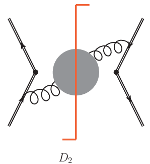
At NNLO the situation is more involved; diagrams with two real soft emissions and virtual diagrams with one real soft emission are present. The soft functions and soft anomalous dimensions at NNLO have a scheme dependence, which originates from the ϵ\epsilon-scalar cut bubble contributing to the second diagram in Figure 2. The grey blob represents the quark, gluon, ghosts and ϵ\epsilon-scalar contributions. The latter is present only in fdh and dred. After calculating the non-vanishing integrals using the techniques described in [54, 55] and summing all the contributions we obtain the NNLO coefficient in Eq. (38) in fdh/dred,

S¯20​(ω)\displaystyle\bar{S}_{20}(\omega) =1ω​CR​[CA​S¯A+NF​TR​S¯f+CR​S¯R],\displaystyle=\frac{1}{\omega}C_{R}\left[C_{A}\,\bar{S}_{A}+N_{F}T_{R}\,\bar{S}_{f}+C_{R}\,\bar{S}_{R}\right]\,, (41)

with

S¯A\displaystyle\bar{S}_{A} =1ϵ2​(−443+2​Nϵ3)+1ϵ​(16​Nϵ9+4​π23−2689)−7​π2​Nϵ9+104​Nϵ27\displaystyle=\frac{1}{\epsilon^{2}}\left(-\frac{44}{3}+\frac{2N_{\epsilon}}{3}\right)+\frac{1}{\epsilon}\left(\frac{16N_{\epsilon}}{9}+\frac{4\pi^{2}}{3}-\frac{268}{9}\right)-\frac{7\pi^{2}N_{\epsilon}}{9}+\frac{104N_{\epsilon}}{27}\,
+56​ζ3+154​π29−161627+(−124​Nϵ​ζ39−56​π2​Nϵ27CLOSE\displaystyle+56\zeta_{3}+\frac{154\pi^{2}}{9}-\frac{1616}{27}+\bigg(-\frac{124N_{\epsilon}\zeta_{3}}{9}-\frac{56\pi^{2}N_{\epsilon}}{27}
OPEN+640​Nϵ81+2728​ζ39−4​π49+938​π227−971281)​ϵ+𝒪⁡(ϵ2),\displaystyle+\frac{640N_{\epsilon}}{81}+\frac{2728\zeta_{3}}{9}-\frac{4\pi^{4}}{9}+\frac{938\pi^{2}}{27}-\frac{9712}{81}\bigg)\epsilon+\mathcal{O}(\epsilon^{2})\,, (42a)
S¯f\displaystyle\bar{S}_{f} =163​ϵ2+809​ϵ−56​π29+44827+(−992​ζ39+262481−280​π227)​ϵ+𝒪⁡(ϵ2),\displaystyle=\frac{16}{3\epsilon^{2}}+\frac{80}{9\epsilon}-\frac{56\pi^{2}}{9}+\frac{448}{27}+\left(-\frac{992\zeta_{3}}{9}+\frac{2624}{81}-\frac{280\pi^{2}}{27}\right)\epsilon+\mathcal{O}(\epsilon^{2})\,, (42b)
S¯R\displaystyle\bar{S}_{R} =−32ϵ3+112​π23​ϵ+1984​ζ33+4​π4​ϵ5+𝒪⁡(ϵ2),\displaystyle=-\frac{32}{\epsilon^{3}}+\frac{112\pi^{2}}{3\epsilon}+\frac{1984\zeta_{3}}{3}+\frac{4\pi^{4}\epsilon}{5}+\mathcal{O}(\epsilon^{2})\,, (42c)

where CR=CFC_{R}=C_{F} for Drell-Yan and CR=CAC_{R}=C_{A} for Higgs production.

Refer to caption Refer to caption
Figure 2: Selected non-zero Feynman diagrams contributing to the one-loop and two-loop soft functions. A complete list of diagrams can be found in [47]. Double lines indicate the direction of Wilson lines while the red vertical cut indicates on-shell partons. The scheme dependence originates from the diagram D2D_{2}. Diagrams D2D_{2}, D3D_{3} and D4D_{4} represent double real soft emissions while diagram D5D_{5} represents a single virtual-real emission.

We now turn to the determination of the soft and cusp anomalous dimension from the soft function. In order to do this we need to discuss the singularities of the soft function that remain after coupling renormalization. From the point of view of ordinary QCD computations, these remaining singularities are closely related to IR singularities. However, from the SCET point of view they simply correspond to UV singularities and are to be removed by renormalization within the effective theory. For convenience this is done in Laplace space by introducing the Laplace transformed soft function as

sRS​(κ)=∫0∞d​ω​exp⁡(−ωκ​eγE)​SRS​(ω),\displaystyle s^{{\rm\scriptscriptstyle RS}}(\kappa)=\int^{\infty}_{0}d\omega\exp\left(-\frac{\omega}{\kappa\,e^{\gamma_{E}}}\right)S^{{\rm\scriptscriptstyle RS}}(\omega)\,, (43)

where the integral transform can be easily carried out by using the relation

∫0∞d​ω​exp⁡(−b​ω)​ω−1−n​ϵ=Γ⁡(−n​ϵ)​bn​ϵ.\displaystyle\int^{\infty}_{0}d\omega\exp\left(-b\omega\right)\omega^{-1-n\epsilon}=\Gamma(-n\epsilon)b^{n\epsilon}\,. (44)

The remaining UV divergences of the soft function can be subtracted multiplicatively,

ssubRS​(κ,μ)=ZsRS​(κ,μ)​sbareRS​(κ).\displaystyle s_{\mathrm{sub}}^{{\rm\scriptscriptstyle RS}}(\kappa,\mu)=Z^{{\rm\scriptscriptstyle RS}}_{s}(\kappa,\mu)\,s_{\mathrm{bare}}^{{\rm\scriptscriptstyle RS}}(\kappa)\,. (45)

Like in the case of general amplitudes in Eq. (6) and Eq. (7), the RGE

dd​ln⁡μ​ssubRS​(κ,μ)=d​ZsRS​(κ,μ)d​ln⁡μ​(ZsRS​(κ,μ))−1​ssubRS​(κ,μ)\displaystyle\frac{d}{d\ln\mu}\,s_{\mathrm{sub}}^{{\rm\scriptscriptstyle RS}}(\kappa,\mu)=\frac{d\,Z^{{\rm\scriptscriptstyle RS}}_{s}(\kappa,\mu)}{d\ln\mu}\big(Z^{{\rm\scriptscriptstyle RS}}_{s}(\kappa,\mu)\big)^{-1}\,s_{\mathrm{sub}}^{{\rm\scriptscriptstyle RS}}(\kappa,\mu)\, (46)

holds, and the corresponding anomalous dimension has a structure similar to Eq. (9),

dd​ln⁡μ​ssubRS​(κ,μ)=[−4​ΓcuspRS​Lκ−2​γWRS]​ssubRS​(κ,μ),\displaystyle\frac{d}{d\ln\mu}s_{\mathrm{sub}}^{{\rm\scriptscriptstyle RS}}(\kappa,\mu)=\left[-4\,\Gamma^{{\rm\scriptscriptstyle RS}}_{\mathrm{cusp}}\,L_{\kappa}-2\gamma^{{\rm\scriptscriptstyle RS}}_{W}\right]s_{\mathrm{sub}}^{{\rm\scriptscriptstyle RS}}(\kappa,\mu)\,, (47)

which is derived from the RG invariance of the cross sections in the threshold region in analogy to the cdr case in Ref. [43]. In Eq. (47) we have defined Lκ≡ln⁡(κ/μ)L_{\kappa}\equiv\ln(\kappa/\mu) and CR=CFC_{R}=C_{F} for Drell-Yan and CR=CAC_{R}=C_{A} for Higgs production. Comparison of the previous two equations yields an expression for the fdh renormalization factor Z¯s​(κ,μ)≡ZsFDH​(κ,μ)\bar{Z}_{s}(\kappa,\mu)\equiv Z^{{\rm\scriptscriptstyle FDH}}_{s}(\kappa,\mu) in terms of the soft and cusp anomalous dimensions. This expression has the same structure as Eq. (12), but can be written in a simpler form because up to NNLO the soft function does not depend on αe\alpha_{e} and α4​ϵ\alpha_{4\epsilon}:

ln⁡Z¯s\displaystyle\ln\bar{Z}_{s} =(αs4​π)​[−Γ¯10ϵ2+1ϵ​(2​Γ¯10​Lκ+γ¯10W)]\displaystyle=\left(\frac{\alpha_{s}}{4\pi}\right)\left[-\frac{\bar{\Gamma}_{10}}{\epsilon^{2}}+\frac{1}{\epsilon}\left(2\bar{\Gamma}_{10}L_{\kappa}+\bar{\gamma}^{W}_{10}\right)\right]\, (48)
+(αs4​π)2​[3​β¯20s​Γ¯104​ϵ3−β¯20s2​ϵ2​(2​Γ¯10​Lκ+γ¯10W)−Γ¯204​ϵ2+12​ϵ​(2​Γ¯20​Lκ+γ¯20W)]\displaystyle+\left(\frac{\alpha_{s}}{4\pi}\right)^{2}\left[\frac{3\bar{\beta}^{s}_{20}\bar{\Gamma}_{10}}{4\epsilon^{3}}-\frac{\bar{\beta}^{s}_{20}}{2\epsilon^{2}}\left(2\bar{\Gamma}_{10}L_{\kappa}+\bar{\gamma}^{W}_{10}\right)-\frac{\bar{\Gamma}_{20}}{4\epsilon^{2}}+\frac{1}{2\epsilon}\left(2\,\bar{\Gamma}_{20}L_{\kappa}+\bar{\gamma}^{W}_{20}\right)\right]\,
+𝒪⁡(αs3).\displaystyle+\mathcal{O}(\alpha^{3}_{s})\,.

By requiring that the renormalization factor Z¯s\bar{Z}_{s} in Eq. (48) minimally subtracts all of the divergences of the bare soft function (in fdh, treating NϵN_{\epsilon} as an independent multiplicity), we extract the expressions for the anomalous dimensions in the fdh scheme

Γ¯cusp\displaystyle\bar{\Gamma}_{\text{cusp}} =(αs4​π)​CR​(4)\displaystyle=\left(\frac{\alpha_{s}}{4\pi}\right)C_{R}\,(4)
+(αs4​π)2​CR​[CA​(2689−43​π2)−809​TR​NF−Nϵ​169​CA]+𝒪⁡(α3),\displaystyle+\Big(\frac{\alpha_{s}}{4\pi}\Big)^{2}\,C_{R}\Big[C_{A}\Big(\frac{268}{9}-\frac{4}{3}\pi^{2}\Big)-\frac{80}{9}T_{R}N_{F}-N_{\epsilon}\frac{16}{9}C_{A}\Big]+\mathcal{O}(\alpha^{3})\,, (49a)
γ¯W\displaystyle\bar{\gamma}_{W} =(αs4​π)2​CR​[CA​(−80827+119​π2+28​ζ3+Nϵ​5227−Nϵ​π218)+TR​NF​(22427−49​π2)]\displaystyle=\Big(\frac{\alpha_{s}}{4\pi}\Big)^{2}C_{R}\bigg[C_{A}\Big(-\frac{808}{27}+\frac{11}{9}\pi^{2}+28\zeta_{3}+N_{\epsilon}\frac{52}{27}-N_{\epsilon}\frac{\pi^{2}}{18}\Big)+T_{R}N_{F}\Big(\frac{224}{27}-\frac{4}{9}\pi^{2}\Big)\bigg]
+𝒪⁡(α3).\displaystyle+\mathcal{O}(\alpha^{3})\,. (49b)

The fact that Γ¯cusp=CR​γ¯cusp\bar{\Gamma}_{\rm cusp}=C_{R}\bar{\gamma}_{\textrm{cusp}}, with the known expression of the cusp anomalous dimension in the fdh scheme, γ¯cusp\bar{\gamma}_{\textrm{cusp}}, is a consistency check of the method. γ¯W\bar{\gamma}_{W} is a new result. The corresponding expressions in cdr/hv can be obtained by simply using the appropriate β\beta functions and anomalous dimensions in Eq. (48) and by setting Nϵ=0N_{\epsilon}=0 in Eq. (49). They are consistent with the literature [43].

Finally we remark that in analogy to Eq. (5) we can obtain a finite and scheme independent soft function sfins_{\mathrm{fin}} through

sfin​(κ,μ)=lim(N)ϵ→0ssubRS​(κ,μ).\displaystyle s_{\mathrm{fin}}(\kappa,\mu)=\lim\limits_{(N)_{\epsilon}\to 0}s_{\mathrm{sub}}^{{\rm\scriptscriptstyle RS}}(\kappa,\mu)\,. (50)

The explicit expression for sfins_{\mathrm{fin}} is given in Eq. (103) of Appendix A.

3.3 Computation and scheme dependence of the quark jet function and γJ​q\gamma_{Jq}

The quark jet function has been calculated at NNLO in cdr [28]. Referring to [28] for more details, we describe here the corresponding calculation in fdh (which is identical to the one in dred, but for simplicity we will only refer to fdh in the present subsection). The jet function is given in terms of the hard-collinear quark propagator

n/2​n¯⋅p​𝒥qRS​(p2)\displaystyle\frac{n\hskip-6.25958pt/\penalty}{2}\;\bar{n}\cdot p\,\mathcal{J}^{{\rm\scriptscriptstyle RS}}_{q}(p^{2}) =∫d4​x​ei​p​x​⟨0|T⁡{χh​c​(x)​χ¯h​c​(0)}|0⟩\displaystyle=\int d^{4}x\,e^{ipx}\langle 0|T\{\chi_{hc}(x)\bar{\chi}_{hc}(0)\}|0\rangle
=∫d4​x​ei​p​x​⟨0|T⁡{n/n¯/4​W†​(x)​ψ​(x)​ψ¯​(0)​W​(0)​n¯/n/4}|0⟩,\displaystyle=\int d^{4}x\,e^{ipx}\langle 0|T\{\frac{n\hskip-6.25958pt/\penalty\,\bar{n}\hskip-6.25958pt/\penalty}{4}W^{\dagger}(x)\psi(x)\bar{\psi}(0)W(0)\frac{\bar{n}\hskip-6.25958pt/\penalty\,n\hskip-6.25958pt/\penalty}{4}\}|0\rangle\,, (51)

with Wilson lines

W⁡(x)=𝒫​exp⁡(i​gs​∫−∞0d​s​n¯⋅A⁡(x+s​n¯)),W(x)=\mathcal{P}\,\exp\Big(ig_{s}\int_{-\infty}^{0}ds\,\bar{n}\,\cdot\,A(x+s\bar{n})\Big)\,, (52)

where Aμ=Aaμ​taA^{\mu}=A^{\mu}_{a}\,t^{a}. The field χh​c​(x)\chi_{hc}(x) is the gauge-invariant (under both soft and hard-collinear gauge transformations) effective-theory field for a massless quark after a decoupling transformation has been applied, which removes the interactions of soft gluons with hard-collinear fields in the leading-power SCET Lagrangian. As shown in Eq. (51), we can rewrite the propagator in terms of standard QCD fields.

The hard-collinear quark propagator 𝒥qRS\mathcal{J}_{q}^{{\rm\scriptscriptstyle RS}} as defined in Eq. (51) is scheme dependent. The fields χh​c\chi_{hc} and ψ\psi on the r.h.s. of Eq. (51) are Heisenberg fields, so applying the usual perturbative expansion results in loop diagrams contributing to the propagator. The scheme dependence is related to UV singularities of such diagrams. Examples of two-loop diagrams are shown in Figure 3. In fdh the computation is similar to the cdr scheme. However there are additional diagrams, which include the ϵ\epsilon-scalars and also depend on the coupling αe\alpha_{e}. An example of a two-loop diagram needed for the jet function in fdh (and not present in the cdr scheme) is shown in Figure 3 (b)(b). Since n¯\bar{n} is a DD-dimensional vector, there are no ϵ\epsilon-scalars originating from the Wilson lines. Indeed, the scalar product in Eq. (52) will vanish in the case of the ϵ\epsilon-scalar.

Refer to caption
Figure 3: Examples of two-loop diagrams contributing to the quark jet function. Gluons emitted from the crossed circles originate from the Wilson lines. Diagram (a) contributes in cdr and fdh, whereas diagram (b) with two ϵ\epsilon-scalars contributes only in fdh.

The jet function JqRS​(p2)J_{q}^{{\rm\scriptscriptstyle RS}}(p^{2}) is the discontinuity of the propagator, i.e.

JqRS​(p2)=1π​Im​[i​𝒥qRS​(p2)].J_{q}^{{\rm\scriptscriptstyle RS}}(p^{2})=\frac{1}{\pi}\text{Im}\Big[i\,\mathcal{J}_{q}^{{\rm\scriptscriptstyle RS}}(p^{2})\Big]\,. (53)

To highlight the similarities with the discussion in Section 2 and the soft function it is convenient to work in Laplace space, so we define ȷqRS​(Q2)\jmath_{q}^{{\rm\scriptscriptstyle RS}}(Q^{2}), the Laplace transform of the jet function as

ȷqRS​(Q2)≡∫0∞d​p2​exp⁡(−p2Q2​eγE)​JqRS​(p2).\jmath_{q}^{{\rm\scriptscriptstyle RS}}(Q^{2})\equiv\int_{0}^{\infty}dp^{2}\,\exp\left(-\frac{p^{2}}{Q^{2}e^{\gamma_{E}}}\right)J_{q}^{{\rm\scriptscriptstyle RS}}(p^{2})\,. (54)

The analogous equation in the case of the soft function is Eq. (43).

To compute the propagator in the fdh scheme, 𝒥¯q​(p2)\bar{\mathcal{J}}_{q}(p^{2}), the diagrams have been generated with QGRAF [56] and the colour algebra has been done with ColorMath [57]. For the reduction of the integrals Reduze 2 [58] has been used. The master integrals needed for the fdh jet function are the same as for the cdr scheme. After taking the imaginary part and performing the Laplace transform, the bare quark jet function at NNLO in fdh is obtained as

ȷ¯q​bare​(Q2)\displaystyle\bar{\jmath}_{q\,\text{bare}}(Q^{2}) =1+as​(Q2)​CF​(4ϵ2+3ϵ+7−2​π23+ϵ⁡(14−π22−8​ζ3))\displaystyle=1+a_{s}(Q^{2})\,C_{F}\,\Big(\frac{4}{\epsilon^{2}}+\frac{3}{\epsilon}+7-\frac{2\,\pi^{2}}{3}+\epsilon\big(14-\frac{\pi^{2}}{2}-8\zeta_{3}\big)\Big)
+ae​(Q2)​CF​Nϵ​(−12​ϵ−1+ϵ⁡(−2+π212))\displaystyle+a_{e}(Q^{2})\,C_{F}\,N_{\epsilon}\,\Big(-\frac{1}{2\,\epsilon}-1+\epsilon\big(-2+\frac{\pi^{2}}{12}\big)\Big)
+as2​(Q2)​(CF2​ȷ¯20q;F+CF​CA​ȷ¯20q;A+CF​TR​NF​ȷ¯20q;f)\displaystyle+a_{s}^{2}(Q^{2})\,\Big(C^{2}_{F}\,\bar{\jmath}^{\,q;F}_{20}+C_{F}C_{A}\,\bar{\jmath}^{\,q;A}_{20}+C_{F}T_{R}N_{F}\,\bar{\jmath}^{\,q;f}_{20}\Big)\phantom{\frac{1}{1}}
+ae2​(Q2)​(CF2​ȷ¯02q;F+CF​CA​ȷ¯02q;A+CF​TR​NF​ȷ¯02q;f)\displaystyle+a_{e}^{2}(Q^{2})\,\Big(C^{2}_{F}\,\bar{\jmath}^{\,q;F}_{02}+C_{F}C_{A}\,\bar{\jmath}^{\,q;A}_{02}+C_{F}T_{R}N_{F}\,\bar{\jmath}^{\,q;f}_{02}\Big)\phantom{\frac{1}{1}}
+as​(Q2)​ae​(Q2)​(CF2​ȷ¯11q;F+CF​CA​ȷ¯11q;A)+𝒪⁡(a3).\displaystyle+a_{s}(Q^{2})a_{e}(Q^{2})\,\Big(C^{2}_{F}\,\bar{\jmath}^{\,q;F}_{11}+C_{F}C_{A}\,\bar{\jmath}^{\,q;A}_{11}\Big)+{\cal O}(a^{3})\,.\phantom{\frac{1}{1}} (55)

In analogy to Eq. (39) we have defined

as​(Q2)≡e−ϵ​γE​(4​π)ϵ​(1Q2)ϵ​αsbare4​π=(μ2Q2)ϵ​Z¯αs​αs(4​π).\displaystyle a_{s}(Q^{2})\equiv e^{-\epsilon\gamma_{E}}(4\pi)^{\epsilon}\,\left(\frac{1}{Q^{2}}\right)^{\epsilon}\frac{\alpha^{\text{bare}}_{s}}{4\pi}=\left(\frac{\mu^{2}}{Q^{2}}\right)^{\epsilon}\frac{\bar{Z}_{\alpha_{s}}\alpha_{s}}{(4\pi)}\,. (56)

with an analogous equation for aea_{e}. The explicit expression for the two-loop coefficients are given in Appendix A. Note that ȷ¯q​bare​(Q2)\bar{\jmath}_{q\,\text{bare}}(Q^{2}) is independent of μ\mu.

The renormalization procedure in any regularization scheme can easily be generalized from the corresponding procedure in cdr [28]. A renormalization factor ZJqRS​(Q2,μ)Z_{J_{q}}^{{\rm\scriptscriptstyle RS}}(Q^{2},\mu) absorbing the UV divergences of the bare jet function is introduced such that

ȷq​subRS​(Q2,μ)=ZJqRS​(Q2,μ)​ȷq​bareRS​(Q2)\jmath_{q\,\text{sub}}^{{\rm\scriptscriptstyle RS}}(Q^{2},\mu)=Z_{J_{q}}^{{\rm\scriptscriptstyle RS}}(Q^{2},\mu)\,\jmath_{q\,\text{bare}}^{{\rm\scriptscriptstyle RS}}(Q^{2}) (57)

is finite. This equation is analogous to Eqs. (4) and (45). Requiring minimal subtraction with NϵN_{\epsilon} as an independent multiplicity determines the explicit form of ZJqRS​(Q2,μ)Z_{J_{q}}^{{\rm\scriptscriptstyle RS}}(Q^{2},\mu) uniquely in terms of the bare quark jet function ȷ¯q​bare​(Q2)\bar{\jmath}_{q\,\text{bare}}(Q^{2}). In principle, ZJqRSZ_{J_{q}}^{{\rm\scriptscriptstyle RS}} depends on all couplings {α}\{\alpha\}. However, in fdh, up to NNLO there is no dependence on α4​ϵ\alpha_{4\epsilon}.

To relate ZJqRS​(Q2,μ)Z_{J_{q}}^{{\rm\scriptscriptstyle RS}}(Q^{2},\mu) to the cusp anomalous dimension γcuspRS\gamma_{\textrm{cusp}}^{{\rm\scriptscriptstyle RS}} and the quark jet anomalous dimension γJqRS\gamma_{J_{q}}^{{\rm\scriptscriptstyle RS}} we follow the same procedure as for the soft anomalous dimension. We compare the RGE of the quark jet function in the form

dd​ln⁡μ​ȷq​subRS​(Q2,μ)=d​ZJqRS​(Q2,μ)d​ln⁡μ​(ZJqRS​(Q2,μ))−1​ȷq​subRS​(Q2,μ)\displaystyle\frac{d}{d\ln\mu}\,\jmath_{q\,\text{sub}}^{{\rm\scriptscriptstyle RS}}(Q^{2},\mu)=\frac{d\,Z^{{\rm\scriptscriptstyle RS}}_{J_{q}}(Q^{2},\mu)}{d\ln\mu}\left(Z^{{\rm\scriptscriptstyle RS}}_{J_{q}}(Q^{2},\mu)\right)^{-1}\,\jmath_{q\,\text{sub}}^{{\rm\scriptscriptstyle RS}}(Q^{2},\mu)\, (58)

to the RGE written in terms of ΓcuspRS\Gamma_{\textrm{cusp}}^{{\rm\scriptscriptstyle RS}} and γJqRS\gamma_{J_{q}}^{{\rm\scriptscriptstyle RS}},

dd​ln⁡μ​ȷq​subRS​(Q2,μ)\displaystyle\frac{d}{d\ln\mu}\jmath_{q\,\text{sub}}^{{\rm\scriptscriptstyle RS}}(Q^{2},\mu) =[−2​ΓcuspRS​LQ−2​γJqRS]​ȷq​subRS​(Q2,μ).\displaystyle=\left[-2\Gamma_{\text{cusp}}^{{\rm\scriptscriptstyle RS}}\,L_{Q}-2\gamma_{J_{q}}^{{\rm\scriptscriptstyle RS}}\right]\jmath_{q\,\text{sub}}^{{\rm\scriptscriptstyle RS}}(Q^{2},\mu)\,. (59)

This relation is analogous to Eqs. (6) and (47); we have used LQ≡ln⁡(Q2/μ2)L_{Q}\equiv\ln(Q^{2}/\mu^{2}) and ΓcuspRS=CF​γcuspRS\Gamma_{\text{cusp}}^{{\rm\scriptscriptstyle RS}}=C_{F}\gamma_{\text{cusp}}^{{\rm\scriptscriptstyle RS}}. With the help of Eqs. (58) and (59) we can express Z¯Jq\bar{Z}_{J_{q}} in terms of the fdh anomalous dimensions. Up to NNLO, the expression for ln⁡Z¯Jq\ln\,\bar{Z}_{J_{q}} has the same structure as Eqs. (12) and (48). We write it explicitly, using that up to NNLO only the two couplings αs\alpha_{s} and αe\alpha_{e} appear:

ln⁡Z¯Jq\displaystyle\ln\bar{Z}_{J_{q}} =αs4​π​[−Γ¯10ϵ2+1ϵ​(Γ¯10​LQ+γ¯10Jq)]+αe4​π​[−Γ¯01ϵ2+1ϵ​(Γ¯01​LQ+γ¯01Jq)]\displaystyle=\frac{\alpha_{s}}{4\pi}\Big[-\frac{\bar{\Gamma}_{10}}{\epsilon^{2}}+\frac{1}{\epsilon}\Big(\bar{\Gamma}_{10}\,L_{Q}+\bar{\gamma}_{10}^{J_{q}}\Big)\Big]+\frac{\alpha_{e}}{4\pi}\Big[-\frac{\bar{\Gamma}_{01}}{\epsilon^{2}}+\frac{1}{\epsilon}\Big(\bar{\Gamma}_{01}\,L_{Q}+\bar{\gamma}_{01}^{J_{q}}\Big)\Big]
+(αs4​π)2[3​(β¯20s​Γ¯10+β¯20e​Γ¯01)4​ϵ3−β¯20s2​ϵ2(Γ¯10LQ+γ¯10Jq)−β¯20e2​ϵ2(Γ¯01LQ+γ¯01Jq)\displaystyle+\big(\frac{\alpha_{s}}{4\pi}\big)^{2}\Big[\,\frac{3\,\big(\bar{\beta}^{s}_{20}\bar{\Gamma}_{10}+\bar{\beta}^{e}_{20}\bar{\Gamma}_{01}\big)}{4\epsilon^{3}}-\frac{\bar{\beta}^{s}_{20}}{2\,\epsilon^{2}}\Big(\bar{\Gamma}_{10}\,L_{Q}+\bar{\gamma}_{10}^{J_{q}}\Big)-\frac{\bar{\beta}^{e}_{20}}{2\,\epsilon^{2}}\Big(\bar{\Gamma}_{01}\,L_{Q}+\bar{\gamma}_{01}^{J_{q}}\Big)
−Γ¯204​ϵ2+12​ϵ(Γ¯20LQ+γ¯20Jq)]\displaystyle\qquad\qquad-\frac{\bar{\Gamma}_{20}}{4\,\epsilon^{2}}+\frac{1}{2\,\epsilon}\Big(\bar{\Gamma}_{20}\,L_{Q}+\bar{\gamma}_{20}^{J_{q}}\Big)\Big]
+(αe4​π)2[3​(β¯02s​Γ¯10+β¯02e​Γ¯01)4​ϵ3−β¯02s2​ϵ2(Γ¯10LQ+γ¯10Jq)−β¯02e2​ϵ2(Γ¯01LQ+γ¯01Jq)\displaystyle+\big(\frac{\alpha_{e}}{4\pi}\big)^{2}\Big[\,\frac{3\,\big(\bar{\beta}^{s}_{02}\bar{\Gamma}_{10}+\bar{\beta}^{e}_{02}\bar{\Gamma}_{01}\big)}{4\epsilon^{3}}-\frac{\bar{\beta}^{s}_{02}}{2\,\epsilon^{2}}\Big(\bar{\Gamma}_{10}\,L_{Q}+\bar{\gamma}_{10}^{J_{q}}\Big)-\frac{\bar{\beta}^{e}_{02}}{2\,\epsilon^{2}}\Big(\bar{\Gamma}_{01}\,L_{Q}+\bar{\gamma}_{01}^{J_{q}}\Big)
−Γ¯024​ϵ2+12​ϵ(Γ¯02LQ+γ¯02Jq)]\displaystyle\qquad\qquad-\frac{\bar{\Gamma}_{02}}{4\,\epsilon^{2}}+\frac{1}{2\,\epsilon}\Big(\bar{\Gamma}_{02}\,L_{Q}+\bar{\gamma}_{02}^{J_{q}}\Big)\Big]
+(αs4​π)(αe4​π)[3​(β¯11s​Γ¯10+β¯11e​Γ¯01)4​ϵ3−β¯11s2​ϵ2(Γ¯10LQ+γ¯10Jq)−β¯11e2​ϵ2(Γ¯01LQ+γ01Jq)\displaystyle+\left(\frac{\alpha_{s}}{4\pi}\right)\left(\frac{\alpha_{e}}{4\pi}\right)\Big[\,\frac{3\,\big(\bar{\beta}^{s}_{11}\bar{\Gamma}_{10}+\bar{\beta}^{e}_{11}\bar{\Gamma}_{01}\big)}{4\epsilon^{3}}-\frac{\bar{\beta}^{s}_{11}}{2\,\epsilon^{2}}\Big(\bar{\Gamma}_{10}\,L_{Q}+\bar{\gamma}_{10}^{J_{q}}\Big)-\frac{\bar{\beta}^{e}_{11}}{2\,\epsilon^{2}}\Big(\bar{\Gamma}_{01}\,L_{Q}+\gamma_{01}^{J_{q}}\Big)
−Γ¯114​ϵ2+12​ϵ(Γ¯11LQ+γ¯11Jq)]+𝒪(α3).\displaystyle\qquad\qquad-\frac{\bar{\Gamma}_{11}}{4\,\epsilon^{2}}+\frac{1}{2\,\epsilon}\Big(\bar{\Gamma}_{11}\,L_{Q}+\bar{\gamma}_{11}^{J_{q}}\Big)\Big]+{\cal O}(\alpha^{3})\,. (60)

On the one hand this formula gives strong consistency checks. It allows for an independent extraction of the cusp anomalous dimension and the coefficients of the β\beta functions of αs\alpha_{s} and αe\alpha_{e} in the fdh scheme. These coefficients agree with the well-known results in the literature [17, 18].

On the other hand, comparing Eq. (60), in particular the 1/ϵ1/\epsilon pole, to the explicit result for the bare quark jet function allows to read off the anomalous dimension γ¯Jq\bar{\gamma}_{J_{q}}. We obtain the following explicit expression in the fdh scheme:

γ¯Jq\displaystyle\bar{\gamma}_{J_{q}} =(αs4​π)​(−3​CF)+(αe4​π)​Nϵ2​CF\displaystyle=\left(\frac{\alpha_{s}}{4\pi}\right)\,\left(-3\,C_{F}\right)+\left(\frac{\alpha_{e}}{4\pi}\right)\,\frac{N_{\epsilon}}{2}\,C_{F}
+(αs4​π)2[CF2(−32+2π2−24ζ3)+CFCA(−176954−11​π29+40ζ3)\displaystyle+\left(\frac{\alpha_{s}}{4\pi}\right)^{2}\,\Big[C_{F}^{2}\Big(-\frac{3}{2}+2\pi^{2}-24\zeta_{3}\Big)+C_{F}C_{A}\Big(-\frac{1769}{54}-\frac{11\pi^{2}}{9}+40\zeta_{3}\Big)
+CFTRNF(24227+4​π29)+Nϵ2(27154+π29)CFCA]\displaystyle\qquad\qquad+\ C_{F}T_{R}N_{F}\Big(\frac{242}{27}+\frac{4\pi^{2}}{9}\Big)+\frac{N_{\epsilon}}{2}\,\Big(\frac{271}{54}+\frac{\pi^{2}}{9}\Big)C_{F}C_{A}\Big]
+(αs4​π)​(αe4​π)​[Nϵ2​(11​CF​CA−4​CF2−23​CF2​π2)]\displaystyle+\left(\frac{\alpha_{s}}{4\pi}\right)\left(\frac{\alpha_{e}}{4\pi}\right)\Big[\frac{N_{\epsilon}}{2}\,\Big(11C_{F}C_{A}-4C_{F}^{2}-\frac{2}{3}C_{F}^{2}\pi^{2}\Big)\Big]
+(αe4​π)2​[−Nϵ28​CF2−3​Nϵ2​CF​TR​NF]+𝒪⁡(α3).\displaystyle+\left(\frac{\alpha_{e}}{4\pi}\right)^{2}\,\Big[-\frac{N_{\epsilon}^{2}}{8}C_{F}^{2}-\frac{3\,N_{\epsilon}}{2}\,C_{F}T_{R}N_{F}\Big]+{\cal O}(\alpha^{3})\,. (61)

Using this expression together with Eqs. (27) and (49b) the quark anomalous dimension in the fdh scheme, γ¯q\bar{\gamma}_{q} can be found. Thus the computation of the soft and quark jet functions provides an alternative determination of γ¯q\bar{\gamma}_{q}. The result agrees with previous determinations [17, 18] and is listed in Appendix B for completeness. Of course, setting Nϵ=0N_{\epsilon}=0 only the pure αs\alpha_{s} terms survive and the well known results in the cdr/hv scheme are recovered.

This is also true for the quark jet function as a whole. In analogy to Eq. (50) we can define

ȷq​fin​(Q2,μ)=lim(N)ϵ→0ȷq​subRS​(Q2,μ),\jmath_{q\,\text{fin}}(Q^{2},\mu)=\lim_{(N)_{\epsilon}\to 0}\jmath_{q\,\text{sub}}^{{\rm\scriptscriptstyle RS}}(Q^{2},\mu)\,, (62)

so the finite quark jet function is scheme independent and can be obtained using any of the regularization schemes. The explicit result is given in Appendix A.

3.4 Computation and scheme dependence of the gluon jet function and γJ​g\gamma_{Jg}

The discussion of the previous subsection can be readily adapted to the gluon case. We closely follow Ref. [29], where the gluon jet function Jg​(p2)J_{g}(p^{2}) has been calculated at NNLO in cdr. The starting point is the gauge-invariant field 𝒜μ\mathcal{A}^{\mu}, related to the collinear gluon field Acμ​(x)A^{\mu}_{c}(x) through

𝒜μ​(x)=𝒜a​μ​(x)​ta=W†​(x)​[i​Dcμ​W​(x)].\mathcal{A}^{\mu}(x)=\mathcal{A}^{a\mu}(x)t_{a}=W^{\dagger}(x)[iD_{c}^{\mu}W(x)]\,. (63)

The treatment of this vector field depends on the regularization scheme; we will give the details below. In all schemes the field 𝒜μ\mathcal{A}^{\mu} satisfies n¯⋅𝒜=0\bar{n}\cdot\mathcal{A}=0; hence it can be decomposed as 𝒜μ=𝒜⟂μ+(n⋅𝒜)​n¯μ/2\mathcal{A}^{\mu}=\mathcal{A}^{\mu}_{\perp}+(n\cdot\mathcal{A})\bar{n}^{\mu}/2 and the leading term is 𝒜⟂μ\mathcal{A}^{\mu}_{\perp}. The gluon jet propagator 𝒥g​(p2)\mathcal{J}_{g}(p^{2}) is then defined as

δa​b​gs2​(−g⟂μ​ν)​𝒥gRS​(p2)=∫d4​x​ei​p​x​⟨0|T⁡{𝒜⟂a​μ​(x)​𝒜⟂b​ν​(0)}|0⟩.\displaystyle\delta^{ab}g_{s}^{2}\left(-g^{\mu\nu}_{\perp}\right)\mathcal{J}^{{\rm\scriptscriptstyle RS}}_{g}(p^{2})=\int d^{4}x\,e^{ipx}\langle 0|T\{\mathcal{A}_{\perp}^{a\mu}(x)\mathcal{A}_{\perp}^{b\nu}(0)\}|0\rangle\,. (64)

For the calculation of 𝒥gRS​(p2)\mathcal{J}^{{\rm\scriptscriptstyle RS}}_{g}(p^{2}) it is actually more convenient to use an equivalent definition in terms of the time-ordered product of the full fields 𝒜μ\mathcal{A}^{\mu},

δa​b​gs2​[(−gμ​ν+n¯μ​pν+pμ​n¯νn¯⋅p)​𝒥gRS​(p2)+n¯μ​n¯ν(n¯⋅p)2​𝒦gRS​(p2)]\displaystyle\delta^{ab}g_{s}^{2}\Big[\Big(-g_{\mu\nu}+\frac{\bar{n}_{\mu}p_{\nu}+p_{\mu}\bar{n}_{\nu}}{\bar{n}\cdot p}\Big)\mathcal{J}^{{\rm\scriptscriptstyle RS}}_{g}(p^{2})+\frac{\bar{n}_{\mu}\bar{n}_{\nu}}{(\bar{n}\cdot p)^{2}}\mathcal{K}^{{\rm\scriptscriptstyle RS}}_{g}(p^{2})\Big] (65)
=∫d4​x​ei​p​x​⟨0|T⁡{𝒜μa​(x)​𝒜νb​(0)}|0⟩\displaystyle\qquad\qquad=\int d^{4}xe^{ipx}\langle 0|T\{\mathcal{A}_{\mu}^{a}(x)\mathcal{A}_{\nu}^{b}(0)\}|0\rangle

and then extract 𝒥gRS​(p2)\mathcal{J}^{{\rm\scriptscriptstyle RS}}_{g}(p^{2}) using a projection. The gluon jet function JgRS​(p2)J^{{\rm\scriptscriptstyle RS}}_{g}(p^{2}) is the discontinuity of the leading part of the propagator, more precisely JgRS​(p2)=Im​[i​𝒥gRS​(p2)]/πJ^{{\rm\scriptscriptstyle RS}}_{g}(p^{2})=\text{Im}[i\,\mathcal{J}^{{\rm\scriptscriptstyle RS}}_{g}(p^{2})]/\pi. The function KgRSK^{{\rm\scriptscriptstyle RS}}_{g} is related to power-suppressed terms and will not be considered any further in this paper.

As in the case of the quark jet function, after decoupling of the soft fields, the collinear Lagrangian is equivalent to the QCD Lagrangian. Exploiting the gauge invariance of 𝒥gRS\mathcal{J}^{{\rm\scriptscriptstyle RS}}_{g} we work in the light-cone gauge n¯⋅A=0\bar{n}\cdot A=0. This is particularly convenient as in this gauge W⁡(x)=1W(x)=1 and, therefore, no diagrams with additional emission of gluons from the Wilson lines have to be considered. Therefore, for the calculation of 𝒥gRS\mathcal{J}^{{\rm\scriptscriptstyle RS}}_{g} only standard QCD Feynman rules are required. Of course, ghost loops are also absent in this gauge.

Now we give details on the regularization scheme dependence. Typical examples of two-loop diagrams contributing to 𝒥gRS\mathcal{J}^{{\rm\scriptscriptstyle RS}}_{g} are shown in Figure 4. In cdr all gluons are DD-dimensional gluons g^{\hat{g}} and no ϵ\epsilon-scalar diagrams are present. Correspondingly, the metric tensor in Eq. (65) is g^μ​ν\hat{g}^{\mu\nu} in cdr. In hv and fdh the external gluons are understood to be strictly 4-dimensional. Thus, the gluons attached to the Wilson lines in Figure 4 are to be interpreted as g¯\bar{g}, and the metric tensor in Eq. (65) is g¯μ​ν\bar{g}^{\mu\nu} in these schemes. Furthermore, in fdh internal gluons are treated as gg and hence are decomposed into g^{\hat{g}} and g~{\tilde{g}}, as indicated in the left and right panel of Figure 4. In dred the definitions of the present subsection apply to external DD-dimensional gluons g^{\hat{g}}. For these, the calculation and the result are the same as the corresponding fdh calculation, see Eq. (20). Hence for simplicity we will only refer to fdh in the remainder of the subsection.

Refer to caption
Figure 4: Sample two-loop diagrams contributing to the gluon jet function. Diagram (a) is present both in cdr and fdh, diagram (b) including an ϵ\epsilon-scalar contributes only in fdh.

After an explicit calculation of the diagrams in fdh, taking the imaginary part and performing the Laplace transform, we obtain for the bare gluon jet function in fdh

ȷ¯g​bare​(Q2)\displaystyle\bar{\jmath}_{g\,\text{bare}}(Q^{2}) =1+as​(CA​[4ϵ2+113​ϵ+679−2​π23+ϵ⁡(40427−11​π218−8​ζ3)]CLOSE\displaystyle=1+a_{s}\Big(C_{A}\Big[\frac{4}{\epsilon^{2}}+\frac{11}{3\epsilon}+\frac{67}{9}-\frac{2\pi^{2}}{3}+\epsilon\,\big(\frac{404}{27}-\frac{11\pi^{2}}{18}-8\zeta_{3}\big)\Big]
+NF​TR​[−43​ϵ−209+ϵ⁡(2​π29−11227)]\displaystyle\qquad\qquad+N_{F}T_{R}\Big[-\frac{4}{3\epsilon}-\frac{20}{9}+\epsilon\,\big(\frac{2\pi^{2}}{9}-\frac{112}{27}\big)\Big]\
OPEN+Nϵ2​CA​[−13​ϵ−89+ϵ⁡(π218−5227)])\displaystyle\qquad\qquad+\frac{N_{\epsilon}}{2}\,C_{A}\Big[-\frac{1}{3\epsilon}-\frac{8}{9}+\epsilon\big(\frac{\pi^{2}}{18}-\frac{52}{27}\big)\Big]\Big)\
+as2​(CA2​ȷ¯20g;A​A+CA​NF​TR​ȷ¯20g;A​f+CF​NF​TR​ȷ¯20g;F​f+NF2​TR2​ȷ¯20g;f​f)\displaystyle+a_{s}^{2}\,\Big(C_{A}^{2}\,\bar{\jmath}^{\,g;\,AA}_{20}+C_{A}N_{F}T_{R}\,\bar{\jmath}^{\,g;\,Af}_{20}+C_{F}N_{F}T_{R}\,\bar{\jmath}^{\,g;\,Ff}_{20}+N_{F}^{2}T_{R}^{2}\,\bar{\jmath}^{\,g;\,ff}_{20}\Big)\phantom{\frac{1}{1}}
+as​ae​(CA​NF​TR​ȷ¯11g;A​f+CF​NF​TR​ȷ¯11g;F​f)+𝒪⁡(α3).\displaystyle+a_{s}a_{e}\,\Big(C_{A}N_{F}T_{R}\,\bar{\jmath}^{\,g;\,Af}_{11}+C_{F}N_{F}T_{R}\,\bar{\jmath}^{\,g;\,Ff}_{11}\Big)+{\cal O}(\alpha^{3})\,.\phantom{\frac{1}{1}} (66)

The explicit results of the two-loop coefficients are given in Appendix A. In the limit Nϵ→0N_{\epsilon}\to 0 all terms proportional to αe\alpha_{e} vanish and we obtain the results in cdr, in agreement with Ref. [29].

The renormalization procedure is the same as for the quark jet function. In Laplace space, the renormalized gluon jet function in the fdh scheme is obtained by multiplying Eq. (66) by a factor Z¯Jg\bar{Z}_{J_{g}}. This factor is the same as in Eq. (60) apart from the replacement γ¯i​jJq→γ¯i​jJg\bar{\gamma}_{ij}^{J_{q}}\to\bar{\gamma}_{ij}^{J_{g}} and ΓcuspRS=CA​γcuspRS\Gamma_{\text{cusp}}^{{\rm\scriptscriptstyle RS}}=C_{A}\gamma_{\text{cusp}}^{{\rm\scriptscriptstyle RS}}. After renormalization of the coupling, all divergences of the bare gluon jet function have to be absorbed by Z¯Jg​(Q2,μ)\bar{Z}_{J_{g}}(Q^{2},\mu). This allows to determine the anomalous dimension of the gluon jet in the fdh scheme as

γ¯Jg\displaystyle\bar{\gamma}_{J_{g}} =(αs4​π)​(−113​CA+43​NF​TR+Nϵ6​CA)\displaystyle=\left(\frac{\alpha_{s}}{4\pi}\right)\,\left(-\frac{11}{3}C_{A}+\frac{4}{3}N_{F}T_{R}+\frac{N_{\epsilon}}{6}C_{A}\right)
+(αs4​π)2[CA2(−109627+11​π29+16ζ3)+CANFTR(36827−4​π29)+4CFTRNF\displaystyle+\left(\frac{\alpha_{s}}{4\pi}\right)^{2}\,\Big[C_{A}^{2}\Big(-\frac{1096}{27}+\frac{11\pi^{2}}{9}+16\zeta_{3}\Big)+C_{A}N_{F}T_{R}\Big(\frac{368}{27}-\frac{4\pi^{2}}{9}\Big)+4C_{F}T_{R}N_{F}
+Nϵ2(24827−π29)CA2]\displaystyle\qquad\qquad+\frac{N_{\epsilon}}{2}\Big(\frac{248}{27}-\frac{\pi^{2}}{9}\Big)C_{A}^{2}\Big]
+(αs4​π)​(αe4​π)​[−Nϵ​(2​CF​NF​TR)]+𝒪⁡(α3).\displaystyle+\left(\frac{\alpha_{s}}{4\pi}\right)\left(\frac{\alpha_{e}}{4\pi}\right)\Big[-N_{\epsilon}\,(2\,C_{F}N_{F}T_{R})\Big]+{\cal O}(\alpha^{3})\,. (67)

Of course, it is again also possible to extract the cusp anomalous dimension as well as the β\beta functions of αs\alpha_{s} and αe\alpha_{e} from Z¯Jg​(Q2,μ)\bar{Z}_{J_{g}}(Q^{2},\mu). The fact that we obtain again the same results for these quantities is a strong consistency check on the procedure.

From γ¯Jg\bar{\gamma}_{J_{g}} we can determine γ¯g\bar{\gamma}_{g} with the help of Eq. (27). The result is in agreement with previous determinations [17, 18] and is listed in Appendix B for completeness, but the present procedure provides a more direct alternative determination of γ¯g\bar{\gamma}_{g}.

Finally, as for the soft and quark jet function, we can obtain a finite and scheme independent gluon jet function as

ȷg​fin​(Q2,μ)=lim(N)ϵ→0ȷg​subRS​(Q2,μ).\jmath_{g\,\text{fin}}(Q^{2},\mu)=\lim_{(N)_{\epsilon}\to 0}\jmath_{g\,\text{sub}}^{{\rm\scriptscriptstyle RS}}(Q^{2},\mu)\,. (68)

For completeness the explicit result is listed in Appendix A.

3.5 Computation of the ϵ\epsilon-scalar jet function, γJ​ϵ\gamma_{J\epsilon} and result for γ¯ϵ\bar{\gamma}_{\epsilon} in DRED

In dred processes with external ϵ\epsilon-scalars need to be considered. The discussion of Section 3.1 applies analogously, and we can determine the anomalous dimension of ϵ\epsilon-scalars from an equation like Eq. (27),

γg~DRED≡γ¯ϵ=γ¯Jϵ−γWϵDRED2.\displaystyle\gamma^{{\rm\scriptscriptstyle DRED}}_{{\tilde{g}}}\equiv\bar{\gamma}_{\epsilon}=\bar{\gamma}_{J_{\epsilon}}-\frac{\gamma^{{\rm\scriptscriptstyle DRED}}_{W_{\epsilon}}}{2}\,. (69)

As mentioned in Section 3.2 the soft function is the same as for external gluons, hence γWϵDRED=γ¯W\gamma^{{\rm\scriptscriptstyle DRED}}_{W_{\epsilon}}=\bar{\gamma}_{W}, from Eq. (49b). For γ¯Jϵ\bar{\gamma}_{J_{\epsilon}} an ϵ\epsilon-scalar jet function is needed. Such an object can be defined and computed in close analogy to the calculation of the gluon jet function, with the difference that now the time-ordered product of two fields 𝒜~μ=g~μ​ν​𝒜ν\tilde{\mathcal{A}}_{\mu}={\tilde{g}}_{\mu\nu}\mathcal{A}^{\nu} has to be considered. In light-cone gauge these fields reduce to the ϵ\epsilon-scalar field A~μ\tilde{A}_{\mu}. Starting from the propagator 𝒥¯ϵ​(p2)≡𝒥ϵDRED​(p2)\bar{\mathcal{J}}_{\epsilon}(p^{2})\equiv\mathcal{J}^{{\rm\scriptscriptstyle DRED}}_{\epsilon}(p^{2}) given by

δa​b​gs2​(−g~μ​ν)​𝒥¯ϵ​(p2)=∫d4​x​ei​p​x​⟨0|T⁡{𝒜~μa​(x)​𝒜~νb​(0)}|0⟩\displaystyle\delta^{ab}g_{s}^{2}\left(-\tilde{g}_{\mu\nu}\right)\bar{\mathcal{J}}_{\epsilon}(p^{2})=\int d^{4}xe^{ipx}\langle 0|T\{\tilde{\mathcal{A}}_{\mu}^{a}(x)\tilde{\mathcal{A}}_{\nu}^{b}(0)\}|0\rangle (70)

the ϵ\epsilon-scalar jet function is obtained as J¯ϵ​(p2)=Im​[i​𝒥¯ϵ​(p2)]/π\bar{J}_{\epsilon}(p^{2})=\text{Im}[i\,\bar{\mathcal{J}}_{\epsilon}(p^{2})]/\pi.

Two examples of diagrams contributing (in light-cone gauge) at two-loop order are shown in Figure 5. A new feature is the appearance of the quartic coupling α4​ϵ\alpha_{4\epsilon}. We do not need to distinguish the three different α4​ϵ\alpha_{4\epsilon} since the quartic coupling only appears at the two-loop level and hence the associated renormalization constants and β\beta functions do not appear. The only non-vanishing diagram ∼α4​ϵ2\sim\alpha^{2}_{4\epsilon} is depicted in Figure 5 b.

Refer to caption
Figure 5: Sample two-loop diagrams contributing to the ϵ\epsilon-scalar jet function both. Diagram (a) is proportional to αs​αe\alpha_{s}\alpha_{e} whereas diagram (b) is ∼α4​ϵ2\sim\alpha^{2}_{4\epsilon}

Performing a computation analogous to previous cases, the bare two-loop ϵ\epsilon-scalar jet function in Laplace space is found to be

ȷ¯ϵ​bare​(Q2)\displaystyle\bar{\jmath}_{\epsilon\,\text{bare}}(Q^{2}) =1+as​CA​(4ϵ2+4ϵ+8−2​π23+ϵ⁡(16−2​π23−8​ζ3))\displaystyle=1+a_{s}\,C_{A}\Big(\frac{4}{\epsilon^{2}}+\frac{4}{\epsilon}+8-\frac{2\pi^{2}}{3}+\epsilon\big(16-\frac{2\pi^{2}}{3}-8\zeta_{3}\big)\Big)
+ae​NF​TR​(−2ϵ−4+ϵ⁡(−8+π23))\displaystyle+a_{e}\,N_{F}T_{R}\Big(-\frac{2}{\epsilon}-4+\epsilon\big(-8+\frac{\pi^{2}}{3}\big)\Big)
+as2​(CA2​ȷ¯200ϵ;A​A+CA​NF​TR​ȷ¯200ϵ;A​f)\displaystyle+a_{s}^{2}\,\Big(C_{A}^{2}\,\bar{\jmath}^{\,\epsilon;\,AA}_{200}+C_{A}N_{F}T_{R}\,\bar{\jmath}^{\,\epsilon;\,Af}_{200}\Big)\phantom{\frac{1}{1}}
+ae2​NF​TR​(CA​ȷ¯020ϵ;A​f+CF​ȷ¯020ϵ;F​f+NF​TR​ȷ¯020ϵ;f​f)\displaystyle+a_{e}^{2}\,N_{F}T_{R}\,\Big(C_{A}\,\bar{\jmath}^{\,\epsilon;\,Af}_{020}+C_{F}\,\bar{\jmath}^{\,\epsilon;\,Ff}_{020}+N_{F}T_{R}\,\bar{\jmath}^{\,\epsilon;\,ff}_{020}\Big)\phantom{\frac{1}{1}}
+a4​ϵ2​CA2​ȷ¯002ϵ;A​A\displaystyle+a_{4\epsilon}^{2}\,C_{A}^{2}\,\bar{\jmath}^{\,\epsilon;\,AA}_{002}\phantom{\frac{1}{1}}
+as​ae​NF​TR​(CA​ȷ¯110ϵ;A​f+CF​ȷ¯110ϵ;F​f)+𝒪⁡(a3).\displaystyle+a_{s}a_{e}\,N_{F}T_{R}\,\Big(C_{A}\,\bar{\jmath}^{\,\epsilon;\,Af}_{110}+C_{F}\,\bar{\jmath}^{\,\epsilon;\,Ff}_{110}\Big)+{\cal O}(a^{3})\,.\phantom{\frac{1}{1}} (71)

Due to the presence of α4​ϵ\alpha_{4\epsilon}, the various coefficients have now three labels, with the last one indicating the power of α4​ϵ\alpha_{4\epsilon}. The explicit NNLO expressions are given in Appendix A.

Once more, the UV divergences of the bare jet function are absorbed by a renormalization factor ZϵDRED​(Q2,μ)Z^{\rm\scriptscriptstyle DRED}_{\epsilon}(Q^{2},\mu), which has a structure similar to Eq. (12) or Eqs. (48) and (60). In fact, it can be written as Eq. (18),

ln⁡ZϵDRED\displaystyle\ln Z^{\rm\scriptscriptstyle DRED}_{\epsilon} =(α→4​π)⋅(Γ→1′DRED4​ϵ2+𝚪→1DRED2​ϵ)\displaystyle=\left(\frac{\vec{\alpha}}{4\pi}\right)\cdot\left(\frac{\vec{\Gamma}^{\prime\,{\rm\scriptscriptstyle DRED}}_{1}}{4\epsilon^{2}}+\frac{\vec{\mathbf{\Gamma}}^{{\rm\scriptscriptstyle DRED}}_{1}}{2\epsilon}\right) (72)
+∑Σ=2(αs4​π)m(αe4​π)n(α4​ϵ4​π)k\displaystyle+\sum_{\Sigma=2}\left(\frac{\alpha_{s}}{4\pi}\right)^{m}\left(\frac{\alpha_{e}}{4\pi}\right)^{n}\left(\frac{\alpha_{4\epsilon}}{4\pi}\right)^{k}\,
(−3​β→m​n​kDRED⋅Γ→1′DRED16​ϵ3−β→m​n​kDRED⋅𝚪→1DRED4​ϵ2+Γm​n​k′DRED16​ϵ2+𝚪m​n​kDRED4​ϵ)+𝒪⁡(α3)\displaystyle\quad\Bigg(-\frac{3\vec{\beta}^{{\rm\scriptscriptstyle DRED}}_{mnk}\cdot\vec{\Gamma}^{\prime\,{\rm\scriptscriptstyle DRED}}_{1}}{16\epsilon^{3}}-\frac{\vec{\beta}^{{\rm\scriptscriptstyle DRED}}_{mnk}\cdot\vec{\mathbf{\Gamma}}^{{\rm\scriptscriptstyle DRED}}_{1}}{4\epsilon^{2}}+\frac{\Gamma^{\prime\,{\rm\scriptscriptstyle DRED}}_{mnk}}{16\epsilon^{2}}+\frac{\mathbf{\Gamma}^{{\rm\scriptscriptstyle DRED}}_{mnk}}{4\epsilon}\Bigg)+\mathcal{O}(\alpha^{3})\,

with the identification

Γ′DRED\displaystyle\Gamma^{\prime\,{\rm\scriptscriptstyle DRED}} =−4​CA​γ¯cusp,\displaystyle=-4\,C_{A}\,\bar{\gamma}_{\text{cusp}}, 𝚪DRED\displaystyle\mathbf{\Gamma}^{{\rm\scriptscriptstyle DRED}} =2​CA​γ¯cusp​LQ+2​γ¯Jϵ.\displaystyle=2\,C_{A}\,\bar{\gamma}_{\text{cusp}}\,L_{Q}+2\,\bar{\gamma}_{J_{\epsilon}}\,. (73)

We refrain from using the explicit form of Eq. (60) since the dependence on α4​ϵ\alpha_{4\epsilon} leads to a proliferation of similar terms. The only simplification used is the identification of the couplings α4​ϵ,i\alpha_{4\epsilon,i}, which is possible since the explicit results show that these couplings appear not at one-loop but only in the genuine two-loop coefficients.

By comparing with the explicit result for the ϵ\epsilon-scalar jet function we determine the renormalization factor using minimal subtraction and extract from this the anomalous dimension of the ϵ\epsilon-scalar jet as

γ¯Jϵ\displaystyle\bar{\gamma}_{J_{\epsilon}} =(αs4​π)​(−4​CA)+(αe4​π)​(2​NF​TR)\displaystyle=\left(\frac{\alpha_{s}}{4\pi}\right)\,\left(-4\,C_{A}\right)+\left(\frac{\alpha_{e}}{4\pi}\right)\,\left(2N_{F}T_{R}\right)
+(αs4​π)2​[CA2​(−4603108+13​π29+16​ζ3+Nϵ​337108+Nϵ​π218)+CA​NF​TR​(33827+4​π29)]\displaystyle+\left(\frac{\alpha_{s}}{4\pi}\right)^{2}\,\Big[C_{A}^{2}\Big(-\frac{4603}{108}+\frac{13\pi^{2}}{9}+16\zeta_{3}+N_{\epsilon}\frac{337}{108}+N_{\epsilon}\frac{\pi^{2}}{18}\Big)+C_{A}N_{F}T_{R}\Big(\frac{338}{27}+\frac{4\pi^{2}}{9}\Big)\Big]
+(αs4​π)​(αe4​π)​[10​CF​NF​TR−4​π23​CA​NF​TR]\displaystyle+\left(\frac{\alpha_{s}}{4\pi}\right)\left(\frac{\alpha_{e}}{4\pi}\right)\Big[10\,C_{F}N_{F}T_{R}-\frac{4\pi^{2}}{3}C_{A}N_{F}T_{R}\Big]
+(αe4​π)2​[NF​TR​(2​CA−4​CF−Nϵ​(CA+CF))]\displaystyle+\left(\frac{\alpha_{e}}{4\pi}\right)^{2}\,\Big[N_{F}T_{R}\big(2\,C_{A}-4\,C_{F}-N_{\epsilon}(C_{A}+C_{F})\big)\Big]
+(α4​ϵ4​π)2​[CA2​34​(−1+Nϵ)]+𝒪⁡(α3).\displaystyle+\left(\frac{\alpha_{4\epsilon}}{4\pi}\right)^{2}\,\Big[C_{A}^{2}\frac{3}{4}(-1+N_{\epsilon})\Big]+{\cal O}(\alpha^{3})\,. (74)

Combining this result as prescribed by Eq. (69) with the soft anomalous dimension, which has only αs2\alpha_{s}^{2} contributions, we find the ϵ\epsilon-scalar anomalous dimension

γ¯ϵ\displaystyle\bar{\gamma}_{\epsilon} =(αs4​π)​(−4​CA)+(αe4​π)​(2​NF​TR)\displaystyle=\left(\frac{\alpha_{s}}{4\pi}\right)\,\left(-4\,C_{A}\right)+\left(\frac{\alpha_{e}}{4\pi}\right)\,\left(2N_{F}T_{R}\right)
+(αs4​π)2​[CA2​(−2987108+5​π26+2​ζ3+Nϵ​233108+Nϵ​π212)+CA​NF​TR​(22627+2​π23)]\displaystyle+\left(\frac{\alpha_{s}}{4\pi}\right)^{2}\,\Big[C_{A}^{2}\Big(-\frac{2987}{108}+\frac{5\pi^{2}}{6}+2\zeta_{3}+N_{\epsilon}\frac{233}{108}+N_{\epsilon}\frac{\pi^{2}}{12}\Big)+C_{A}N_{F}T_{R}\Big(\frac{226}{27}+\frac{2\pi^{2}}{3}\Big)\Big]
+(αs4​π)​(αe4​π)​[10​CF​NF​TR−4​π23​CA​NF​TR]\displaystyle+\left(\frac{\alpha_{s}}{4\pi}\right)\left(\frac{\alpha_{e}}{4\pi}\right)\Big[10\,C_{F}N_{F}T_{R}-\frac{4\pi^{2}}{3}C_{A}N_{F}T_{R}\Big]
+(αe4​π)2​[NF​TR​(2​CA−4​CF−Nϵ​(CA+CF))]\displaystyle+\left(\frac{\alpha_{e}}{4\pi}\right)^{2}\,\Big[N_{F}T_{R}\big(2\,C_{A}-4\,C_{F}-N_{\epsilon}(C_{A}+C_{F})\big)\Big]
+(α4​ϵ4​π)2​[CA2​34​(−1+Nϵ)]+𝒪⁡(α3).\displaystyle+\left(\frac{\alpha_{4\epsilon}}{4\pi}\right)^{2}\,\Big[C_{A}^{2}\frac{3}{4}(-1+N_{\epsilon})\Big]+{\cal O}(\alpha^{3})\,. (75)

As discussed in Section 2.3, γ¯ϵ\bar{\gamma}_{\epsilon} is needed to relate two-loop matrix elements computed in dred to those computed in other schemes such as fdh. With this new result all anomalous dimensions are known at the two-loop level in all four schemes.

4 Alternative determination of γ¯ϵ\bar{\gamma}_{\epsilon} from the ϵ\mathbf{\epsilon}-scalar form factor

Apart from the new approach of extracting the IR anomalous dimension of the ϵ\epsilon-scalar, γ¯ϵ\bar{\gamma}_{\epsilon} defined in Eq. (21) from the ϵ\epsilon-scalar jet and soft functions, it is also possible to obtain this quantity in the more traditional way, by comparing the generic infrared factorization formula with a specific amplitude for a process containing external ϵ\epsilon-scalars. This procedure is analogous to the determination of γ¯q\bar{\gamma}_{q} and γ¯g\bar{\gamma}_{g} in Ref. [18]. We now describe the determination of γ¯ϵ\bar{\gamma}_{\epsilon} via a process with two external ϵ\epsilon-scalars, the ϵ\epsilon-scalar form factor, which has been calculated recently in Ref. [31] up to the two-loop level.

According to Eq. (18) the one-loop infrared divergences in the dred scheme are described by

ln​𝐙¯1L=\displaystyle\text{ln}\,\bar{\mathbf{Z}}^{\text{1L}}= (αs4​π)​[−Γ¯1002​ϵ2+γ¯100ϵϵ]+(αe4​π)​[−Γ¯0102​ϵ2+γ¯010ϵϵ]\displaystyle\Big(\frac{\alpha_{s}}{4\pi}\Big)\Bigg[-\frac{\bar{\Gamma}_{100}}{2\epsilon^{2}}+\frac{\bar{\gamma}^{\epsilon}_{100}}{\epsilon}\Bigg]+\Big(\frac{\alpha_{e}}{4\pi}\Big)\Bigg[-\frac{\bar{\Gamma}_{010}}{2\epsilon^{2}}+\frac{\bar{\gamma}^{\epsilon}_{010}}{\epsilon}\Bigg]
+(α4​ϵ4​π)​[−Γ¯0012​ϵ2+γ¯001ϵϵ].\displaystyle+\Big(\frac{\alpha_{4\epsilon}}{4\pi}\Big)\Bigg[-\frac{\bar{\Gamma}_{001}}{2\epsilon^{2}}+\frac{\bar{\gamma}^{\epsilon}_{001}}{\epsilon}\Bigg]. (76)

Here the relations Γ¯′i​j​k=−2Γ¯i​j​k=−2CAγ¯cuspi​j​k\bar{\Gamma}{{}^{\prime}}_{ijk}=-2\,\bar{\Gamma}_{ijk}=-2C_{A}\bar{\gamma}^{\text{cusp}}_{ijk} and 𝚪¯i​j​k=2​γ¯i​j​kϵ\bar{\mathbf{\Gamma}}_{ijk}=2\,\bar{\gamma}^{\epsilon}_{ijk} have been used. The notation with three indices for a common α4​ϵ\alpha_{4\epsilon} coupling and for dropping the superscript “cusp” has been explained in Section 3.1. Eq. (76) can now be compared with the corresponding IR divergent one-loop result of the UV renormalized ϵ\epsilon-scalar form factor given in Ref. [31], where TR=12T_{R}=\frac{1}{2} and μ2=−s12\mu^{2}=-s_{12} has been used:

F¯ϵ1L\displaystyle\bar{F}^{\text{1L}}_{\epsilon} =(αs4​π)​[−2ϵ2−4ϵ]​CA+(αe4​π)​NFϵ+𝒪⁡(ϵ0).\displaystyle=\Big(\frac{\alpha_{s}}{4\pi}\Big)\Bigg[-\frac{2}{\epsilon^{2}}-\frac{4}{\epsilon}\Bigg]C_{A}+\Big(\frac{\alpha_{e}}{4\pi}\Big)\frac{N_{F}}{\epsilon}+\mathcal{O}(\epsilon^{0}). (77)

The 1ϵ2\frac{1}{\epsilon^{2}}-pole of this one-loop form factor confirms the previous finding that the one-loop cusp anomalous dimension is a process-independent quantity that has only one non-vanishing component Γ¯100=4​CA=γ¯100cusp​CA\bar{\Gamma}_{100}=4\,C_{A}=\bar{\gamma}^{\text{cusp}}_{100}\,C_{A}. On the other hand, the 1ϵ\frac{1}{\epsilon}-poles in Eq. (77) are directly correlated with the components of the anomalous dimension γ¯ϵ\bar{\gamma}_{\epsilon}. The values obtained here agree with the results from the previous section.

The appropriate two-loop prediction for ln​𝐙¯2L\text{ln}\,\bar{\mathbf{Z}}^{\text{2L}} could be given in a completely general form, as in Eqs. (18) and (72), in which it would allow to read off once again even the one-loop β\beta functions. Here, however, we give the prediction in a more specific form, where we already use the knowledge that several one-loop coefficients are zero. Considering only non-vanishing components of one-loop anomalous dimensions and β\beta functions yields for the infrared divergence structure at the two-loop level:

ln​𝐙¯2L=\displaystyle\text{ln}\,\bar{\mathbf{Z}}^{\text{2L}}= (αs4​π)2​[3​β¯200s​Γ¯1008​ϵ3−β¯200s​γ¯100ϵ2​ϵ2−Γ¯2008​ϵ2+γ¯200ϵ2​ϵ]\displaystyle\Big(\frac{\alpha_{s}}{4\pi}\Big)^{2}\Bigg[\frac{3\,\bar{\beta}^{s}_{200}\,\bar{\Gamma}_{100}}{8\epsilon^{3}}-\frac{\bar{\beta}^{s}_{200}\,\bar{\gamma}^{\epsilon}_{100}}{2\epsilon^{2}}-\frac{\bar{\Gamma}_{200}}{8\epsilon^{2}}+\frac{\bar{\gamma}^{\epsilon}_{200}}{2\epsilon}\Bigg]
+(αs4​π)​(αe4​π)​[−β¯110e​γ¯010ϵ2​ϵ2−Γ¯1108​ϵ2+γ¯110ϵ2​ϵ]\displaystyle+\Big(\frac{\alpha_{s}}{4\pi}\Big)\Big(\frac{\alpha_{e}}{4\pi}\Big)\Bigg[-\frac{\bar{\beta}^{e}_{110}\,\bar{\gamma}^{\epsilon}_{010}}{2\epsilon^{2}}-\frac{\bar{\Gamma}_{110}}{8\epsilon^{2}}+\frac{\bar{\gamma}^{\epsilon}_{110}}{2\epsilon}\Bigg]
+(αe4​π)2​[−β¯020e​γ¯010ϵ2​ϵ2−Γ¯0208​ϵ2+γ¯020ϵ2​ϵ]+(αs4​π)​(α4​ϵ4​π)​[−Γ¯1018​ϵ2+γ¯101ϵ2​ϵ]\displaystyle+\Big(\frac{\alpha_{e}}{4\pi}\Big)^{2}\,\Bigg[-\frac{\bar{\beta}^{e}_{020}\,\bar{\gamma}^{\epsilon}_{010}}{2\epsilon^{2}}-\frac{\bar{\Gamma}_{020}}{8\epsilon^{2}}+\frac{\bar{\gamma}^{\epsilon}_{020}}{2\epsilon}\Bigg]+\Big(\frac{\alpha_{s}}{4\pi}\Big)\Big(\frac{\alpha_{4\epsilon}}{4\pi}\Big)\Bigg[-\frac{\bar{\Gamma}_{101}}{8\epsilon^{2}}+\frac{\bar{\gamma}^{\epsilon}_{101}}{2\epsilon}\Bigg]
+(αe4​π)​(α4​ϵ4​π)​[−Γ¯0118​ϵ2+γ¯011ϵ2​ϵ]+(α4​ϵ4​π)2​[−Γ¯0028​ϵ2+γ¯002ϵ2​ϵ].\displaystyle+\Big(\frac{\alpha_{e}}{4\pi}\Big)\Big(\frac{\alpha_{4\epsilon}}{4\pi}\Big)\Bigg[-\frac{\bar{\Gamma}_{011}}{8\epsilon^{2}}+\frac{\bar{\gamma}^{\epsilon}_{011}}{2\epsilon}\Bigg]+\Big(\frac{\alpha_{4\epsilon}}{4\pi}\Big)^{2}\Bigg[-\frac{\bar{\Gamma}_{002}}{8\epsilon^{2}}+\frac{\bar{\gamma}^{\epsilon}_{002}}{2\epsilon}\Bigg]\,. (78)

Thanks to the simple colour and momentum structure of the form factor, this has to correspond directly to the divergence structure of the combination F¯ϵ2L−12​(F¯ϵ1L)2\bar{F}^{\text{2L}}_{\epsilon}-\frac{1}{2}(\bar{F}^{\text{1L}}_{\epsilon})^{2}, see Ref. [18]. Inserting the results for the form factor of Ref. [31] yields

F¯ϵ2L\displaystyle\bar{F}^{\text{2L}}_{\epsilon} −12​(F¯ϵ1L)2\displaystyle-\frac{1}{2}\Big(\bar{F}^{\text{1L}}_{\epsilon}\Big)^{2}
=(αs4​π)2{CA2[112−Nϵ4ϵ3+6518+π26−Nϵ9ϵ2+−2987216+5​π212+ζ⁡(3)+Nϵ​(233216+π224)ϵ]\displaystyle=\Big(\frac{\alpha_{s}}{4\pi}\Big)^{2}\Bigg\{C_{A}^{2}\Bigg[\frac{\frac{11}{2}-\frac{N_{\epsilon}}{4}}{\epsilon^{3}}+\frac{\frac{65}{18}+\frac{\pi^{2}}{6}-\frac{N_{\epsilon}}{9}}{\epsilon^{2}}+\frac{-\frac{2987}{216}+\frac{5\pi^{2}}{12}+\zeta(3)+N_{\epsilon}\Big(\frac{233}{216}+\frac{\pi^{2}}{24}\Big)}{\epsilon}\Bigg]
+CANF[−1ϵ3−79​ϵ2+11354+π26ϵ]}\displaystyle\quad\quad\quad\quad\quad+C_{A}N_{F}\Bigg[-\frac{1}{\epsilon^{3}}-\frac{7}{9\epsilon^{2}}+\frac{\frac{113}{54}+\frac{\pi^{2}}{6}}{\epsilon}\Bigg]\Bigg\}
+(αs4​π)​(αe4​π)​{CF​NF​[−3ϵ2+52​ϵ]−CA​NF​π23​ϵ}\displaystyle+\Big(\frac{\alpha_{s}}{4\pi}\Big)\Big(\frac{\alpha_{e}}{4\pi}\Big)\Bigg\{C_{F}N_{F}\Bigg[-\frac{3}{\epsilon^{2}}+\frac{5}{2\epsilon}\Bigg]-C_{A}N_{F}\frac{\pi^{2}}{3\epsilon}\Bigg\}
+(αe4​π)2​{CA​NF​[−1+Nϵ2ϵ2+12−Nϵ4ϵ]+CF​NF​[2−Nϵ2ϵ2+−1−Nϵ4ϵ]+NF2​12​ϵ2}\displaystyle+\Big(\frac{\alpha_{e}}{4\pi}\Big)^{2}\Bigg\{C_{A}N_{F}\Bigg[\frac{-1+\frac{N_{\epsilon}}{2}}{\epsilon^{2}}+\frac{\frac{1}{2}-\frac{N_{\epsilon}}{4}}{\epsilon}\Bigg]+C_{F}N_{F}\Bigg[\frac{2-\frac{N_{\epsilon}}{2}}{\epsilon^{2}}+\frac{-1-\frac{N_{\epsilon}}{4}}{\epsilon}\Bigg]+N_{F}^{2}\frac{1}{2\epsilon^{2}}\Bigg\}
+(α4​ϵ4​π)2​CA2​(1−Nϵ)​−38​ϵ+𝒪⁡(ϵ0).\displaystyle+\Big(\frac{\alpha_{4\epsilon}}{4\pi}\Big)^{2}C_{A}^{2}\,(1-N_{\epsilon})\frac{-3}{8\epsilon}+\mathcal{O}(\epsilon^{0}).\phantom{\Bigg\}} (79)

Again, the 1ϵ\frac{1}{\epsilon}-poles allow to read off the components of the anomalous dimension of the ϵ\epsilon-scalar γ¯ϵ\bar{\gamma}_{\epsilon}. The values found here agree with the results from the previous section, see Eq. (75). Since the remaining divergence structure is governed by one-loop anomalous dimensions, the process-independent components of the cusp anomalous dimension and previously known β\beta coefficients, this is further evidence for the validity of the results obtained in Section 3.5. With this result, and the results of the previous sections and Ref. [18], all two-loop anomalous dimensions γi\gamma_{i} in all rs have been determined both in the SCET approach and from form factors.

5 Cross check with explicit processes

The results of the previous sections allow us to predict the differences between UV renormalized virtual two-loop amplitudes squared, as defined in Eq. (3), computed in different regularization schemes. In this section we will make these transition rules more explicit and will check them with explicit examples.

The following discussions will also shed more light on the role of the various couplings αs\alpha_{s}, αe\alpha_{e} and α4​ϵ,i\alpha_{4\epsilon,i}. In the practical computation of the genuine two-loop diagrams it is no problem to set these couplings equal from the beginning. In the process of UV renormalization, i.e. in lower-order diagrams with counterterm insertions, the bare couplings and the associated renormalization constants appear. It is unavoidable to keep these distinct, regardless whether fdh or dred is used. Once renormalization has been performed, it is possible to set the renormalized couplings equal and to identify NϵN_{\epsilon} and 2​ϵ2\epsilon. Likewise, the derivation of the IR subtraction formulas and the transition rules requires the couplings to be treated independently, but in the end the transition rules can be easily written down for the special case of equal couplings.

We will consider the transition rules fdh ↔\leftrightarrow hv, as well as fdh ↔\leftrightarrow dred. To make connection to the scheme that is used most often, cdr, we remind the reader of the discussion in Section 2.2. The only difference in the squared matrix element between hv and cdr is due to the use of different metric tensors for the polarization sum of external gluons. All anomalous dimensions are the same in the two schemes.

5.1 Transition between FDH and HV

Since external gluons are treated in the same way in fdh and hv, we can actually relate directly virtual amplitudes and do not need to work with squared amplitudes. The finite remainders of the scattering amplitudes are scheme independent. More precisely

|𝒜fin​({p},μ)⟩\displaystyle|\mathcal{A}_{\mathrm{fin}}(\{p\},\mu)\rangle =limϵ→0𝐙−1​(ϵ,{p},μ)​|𝒜⁡(ϵ,{p})⟩\displaystyle=\lim_{\epsilon\to 0}\mathbf{Z}^{-1}(\epsilon,\{p\},\mu)|\mathcal{A}(\epsilon,\{p\})\rangle
=lim(N)ϵ→0𝐙¯−1​(ϵ,Nϵ,{p},μ)​|𝒜¯​(ϵ,Nϵ,{p})⟩,\displaystyle=\lim_{(N)_{\epsilon}\to 0}\bar{\mathbf{Z}}^{-1}(\epsilon,N_{\epsilon},\{p\},\mu)|\bar{\mathcal{A}}(\epsilon,N_{\epsilon},\{p\})\rangle\,, (80)

where |𝒜⟩=|𝒜HV⟩|\mathcal{A}\rangle=|\mathcal{A}^{{\rm\scriptscriptstyle HV}}\rangle and 𝐙=𝐙HV\mathbf{Z}=\mathbf{Z}^{{\rm\scriptscriptstyle HV}} denote quantities in the hv scheme and |𝒜¯⟩=|𝒜FDH⟩|\bar{\mathcal{A}}\rangle=|\mathcal{A}^{{\rm\scriptscriptstyle FDH}}\rangle and 𝐙¯=𝐙FDH\bar{\mathbf{Z}}=\mathbf{Z}^{{\rm\scriptscriptstyle FDH}} are the corresponding quantities in the fdh scheme. Suppressing the arguments of the amplitudes, setting Nϵ=2​ϵN_{\epsilon}=2\epsilon and writing 𝐙−1=1+δ​𝐙\mathbf{Z}^{-1}=1+\delta\mathbf{Z} in both schemes, we can rewrite this equation as

|𝒜⟩\displaystyle|\mathcal{A}\rangle +δ​𝐙​|𝒜⟩=|𝒜¯⟩+δ​𝐙¯​|𝒜¯⟩+𝒪⁡(ϵ).\displaystyle+\delta\mathbf{Z}|\mathcal{A}\rangle=|\bar{\mathcal{A}}\rangle+\delta\bar{\mathbf{Z}}|\bar{\mathcal{A}}\rangle+\mathcal{O}(\epsilon)\,. (81)

If the expansion coefficients δ​Z\delta\textbf{Z} are known to 𝒪⁡(αn)\mathcal{O}(\alpha^{n}) and the amplitudes |𝒜⟩|\mathcal{A}\rangle are known to 𝒪⁡(αn−1)\mathcal{O}(\alpha^{n-1}), this equation allows to obtain a relation between the 𝒪⁡(αn)\mathcal{O}(\alpha^{n}) amplitudes computed in hv and fdh, up to 𝒪⁡(ϵ)\mathcal{O}(\epsilon) terms. We now give the explicit results up to the two-loop level.

The tree-level amplitudes in the two schemes are the same |𝒜¯0⟩=|𝒜0⟩|\bar{\mathcal{A}}_{0}\rangle=|\mathcal{A}_{0}\rangle. At one-loop we can relate the 𝒪⁡(αs)\mathcal{O}({\alpha_{s}}) and 𝒪⁡(αe)\mathcal{O}({\alpha_{e}}) corrections in the fdh scheme, denoted by |𝒜¯10⟩|\bar{\mathcal{A}}_{10}\rangle and |𝒜¯01⟩|\bar{\mathcal{A}}_{01}\rangle respectively, to |𝒜1⟩|\mathcal{A}_{1}\rangle, the 𝒪⁡(αs)\mathcal{O}({\alpha_{s}}) corrections in the hv scheme

|𝒜¯01⟩\displaystyle|\bar{\mathcal{A}}_{01}\rangle =−δ​𝐙¯01​|𝒜0⟩+𝒪⁡(ϵ),\displaystyle=-\delta\bar{\mathbf{Z}}_{01}|\mathcal{A}_{0}\rangle+\mathcal{O}(\epsilon)\,,\phantom{\frac{1}{1}} (82a)
|𝒜¯10⟩−|𝒜1⟩\displaystyle|\bar{\mathcal{A}}_{10}\rangle-|\mathcal{A}_{1}\rangle =(δ​𝐙1−δ​𝐙¯10)​|𝒜0⟩+𝒪⁡(ϵ).\displaystyle=(\delta\mathbf{Z}_{1}-\delta\bar{\mathbf{Z}}_{10})|\mathcal{A}_{0}\rangle+\mathcal{O}(\epsilon)\,.\phantom{\frac{1}{1}} (82b)

In the above equation we have also introduced the expansion coefficients δ​𝐙m\delta\mathbf{Z}_{m} and δ​𝐙¯m​n\delta\bar{\mathbf{Z}}_{mn} of 𝐙−1=1+δ​𝐙\mathbf{Z}^{-1}=1+\delta\mathbf{Z} in the hv and fdh scheme, respectively. Substituting in the last equations the explicit expressions of these expansion coefficients, the explicit form of the differences for a process with #​q\#q external massless quarks and #​g\#g external gluons read

|𝒜¯01⟩\displaystyle|\bar{\mathcal{A}}_{01}\rangle =#​q​γ¯01q2​ϵ​|𝒜0⟩+𝒪⁡(ϵ)=#​q​CF2​|𝒜0⟩+𝒪⁡(ϵ),\displaystyle=\frac{\#q\,\bar{\gamma}^{q}_{01}}{2\epsilon}|\mathcal{A}_{0}\rangle+\mathcal{O}(\epsilon)=\#q\frac{C_{F}}{2}|\mathcal{A}_{0}\rangle+\mathcal{O}(\epsilon)\,, (83a)
|𝒜¯10⟩−|𝒜1⟩\displaystyle|\bar{\mathcal{A}}_{10}\rangle-|\mathcal{A}_{1}\rangle =#​g​(γ¯10g−γ10g)2​ϵ​|𝒜0⟩+𝒪⁡(ϵ)=#​g​CA6​|𝒜0⟩+𝒪⁡(ϵ),\displaystyle=\frac{\#g\,(\bar{\gamma}^{g}_{10}-\gamma^{g}_{10})}{2\epsilon}|\mathcal{A}_{0}\rangle+\mathcal{O}(\epsilon)=\#g\frac{C_{A}}{6}|\mathcal{A}_{0}\rangle+\mathcal{O}(\epsilon)\,, (83b)

which agrees with the results in [16, 4]. In Eq. (83) and what follows we use the notation (see footnote in Section 3.1) γm​0≡γmHV\gamma_{m0}\equiv\gamma_{m}^{{\rm\scriptscriptstyle HV}} for the anomalous dimensions (and the β\beta-functions) in the hv scheme. Since in the hv scheme the anomalous dimensions depend only on αs\alpha_{s} but not on αe\alpha_{e} the second label is always zero. Of course, this is not the case in the corresponding quantities in the fdh scheme, γ¯m​n\bar{\gamma}_{mn}. To obtain Eq. (83) we have used γ10q=γ¯10q\gamma^{q}_{10}=\bar{\gamma}^{q}_{10} and γ10cusp=γ¯10cusp\gamma^{\text{cusp}}_{10}=\bar{\gamma}^{\text{cusp}}_{10}.

Moving to the two-loop level the corresponding equations are

|𝒜¯02⟩\displaystyle|\bar{\mathcal{A}}_{02}\rangle =−δ​𝐙¯01​|𝒜¯01⟩−δ​𝐙¯02​|𝒜0⟩+𝒪⁡(ϵ),\displaystyle=-\delta\bar{\mathbf{Z}}_{01}|\bar{\mathcal{A}}_{01}\rangle-\delta\bar{\mathbf{Z}}_{02}|\mathcal{A}_{0}\rangle+\mathcal{O}(\epsilon)\,,\phantom{\frac{1}{1}} (84a)
|𝒜¯20⟩−|𝒜2⟩\displaystyle|\bar{\mathcal{A}}_{20}\rangle-|\mathcal{A}_{2}\rangle =δ​Z1​|𝒜1⟩−δ​Z¯10​|𝒜¯10⟩+(δ​Z2−δ​Z¯20)​|𝒜0⟩+𝒪⁡(ϵ),\displaystyle=\delta\textbf{Z}_{1}|\mathcal{A}_{1}\rangle-\delta\bar{\textbf{Z}}_{10}|\bar{\mathcal{A}}_{10}\rangle+(\delta\textbf{Z}_{2}-\delta\bar{\textbf{Z}}_{20})|\mathcal{A}_{0}\rangle+\mathcal{O}(\epsilon)\,,\phantom{\frac{1}{1}} (84b)
|𝒜¯11⟩\displaystyle|\bar{\mathcal{A}}_{11}\rangle =−δ​Z¯01​|𝒜¯10⟩−δ​Z¯10​|𝒜¯01⟩−δ​Z¯11​|𝒜0⟩+𝒪⁡(ϵ).\displaystyle=-\delta\bar{\textbf{Z}}_{01}|\bar{\mathcal{A}}_{10}\rangle-\delta\bar{\textbf{Z}}_{10}|\bar{\mathcal{A}}_{01}\rangle-\delta\bar{\textbf{Z}}_{11}|\mathcal{A}_{0}\rangle+\mathcal{O}(\epsilon)\,.\phantom{\frac{1}{1}} (84c)

The expressions given in (84a), (84b) and (84c) allow one to move from fdh to hv (and vice versa) for any process with #​g\#g external gluons and #​q\#q external massless quarks in QCD up to two-loop order. Exploiting γ10q=γ¯10q\gamma^{q}_{10}=\bar{\gamma}^{q}_{10} and γ10cusp=γ¯10cusp\gamma^{\text{cusp}}_{10}=\bar{\gamma}^{\text{cusp}}_{10} we obtain

|𝒜¯02⟩\displaystyle|\mathcal{\bar{A}}_{02}\rangle =[−18​ϵ2​#​q​γ¯01q​(2​β¯02e+#​q​γ¯01q)+14​ϵ​#​q​γ¯02q]​|𝒜0⟩\displaystyle=\bigg[\frac{-1}{8\epsilon^{2}}\#q\bar{\gamma}^{q}_{01}(2\bar{\beta}^{e}_{02}+\#q\bar{\gamma}^{q}_{01})+\frac{1}{4\epsilon}\#q\bar{\gamma}^{q}_{02}\bigg]|\mathcal{A}_{0}\rangle
+[12​ϵ​#​q​γ¯01q]​|𝒜¯01⟩+𝒪⁡(ϵ),\displaystyle+\bigg[\frac{1}{2\epsilon}\#q\bar{\gamma}^{q}_{01}\bigg]|\mathcal{\bar{A}}_{01}\rangle+\mathcal{O}(\epsilon)\,, (85a)
|𝒜¯20⟩−|𝒜2⟩\displaystyle|\mathcal{\bar{A}}_{20}\rangle-|\mathcal{A}_{2}\rangle =[−316​ϵ3[(CA#g+CF#q)(β20s−β¯20s)γ10cusp]\displaystyle=\bigg[\frac{-3}{16\epsilon^{3}}\Big[(C_{A}\#g+C_{F}\#q)(\beta^{s}_{20}-\bar{\beta}^{s}_{20})\gamma^{\text{cusp}}_{10}\Big]
+116​ϵ2[(CA#g+CF#q)(γ20cusp−γ¯20cusp)−2#g(−2β20sγ10g+#g(γ10g−γ¯10g)2\displaystyle+\frac{1}{16\epsilon^{2}}\Big[(C_{A}\#g+C_{F}\#q)(\gamma^{\text{cusp}}_{20}-\bar{\gamma}^{\text{cusp}}_{20})-2\#g(-2\beta^{s}_{20}\gamma^{g}_{10}+\#g(\gamma^{g}_{10}-\bar{\gamma}^{g}_{10})^{2}
+2β¯20sγ¯10g)+(β20s−β¯20s)(4#qγ10q+2γ10cusp∑(i,j)Ti⋅Tjln(μ2−si​j))]\displaystyle+2\bar{\beta}^{s}_{20}\bar{\gamma}^{g}_{10})+(\beta^{s}_{20}-\bar{\beta}^{s}_{20})\Big(4\#q\gamma^{q}_{10}+2\gamma^{\text{cusp}}_{10}\sum_{(i,j)}\textbf{T}_{i}\cdot\textbf{T}_{j}\ln(\frac{\mu^{2}}{-s_{ij}})\Big)\Big]
+18​ϵ[2#g(γ¯20g−γ20g)+2#q(γ¯20q−γ20q)\displaystyle+\frac{1}{8\epsilon}\Big[2\#g(\bar{\gamma}^{g}_{20}-\gamma^{g}_{20})+2\#q(\bar{\gamma}^{q}_{20}-\gamma^{q}_{20})
+(γ¯20cusp−γ20cusp)∑(i,j)Ti⋅Tjln(μ2−si​j)]]|𝒜0⟩\displaystyle\qquad+(\bar{\gamma}^{\text{cusp}}_{20}-\gamma^{\text{cusp}}_{20})\sum_{(i,j)}\textbf{T}_{i}\cdot\textbf{T}_{j}\ln(\frac{\mu^{2}}{-s_{ij}})\Big]\bigg]|\mathcal{A}_{0}\rangle
+[−14​ϵ2(CA#g+CF#q)γ10cusp\displaystyle+\bigg[\frac{-1}{4\epsilon^{2}}(C_{A}\#g+C_{F}\#q)\gamma^{\text{cusp}}_{10}
+14​ϵ(2#gγ¯10g+2#qγ10q+γ10cusp∑(i,j)Ti⋅Tjln(μ2−si​j))]|𝒜10diff⟩\displaystyle+\frac{1}{4\epsilon}\Big(2\#g\bar{\gamma}^{g}_{10}+2\#q\gamma^{q}_{10}+\gamma^{\text{cusp}}_{10}\sum_{(i,j)}\textbf{T}_{i}\cdot\textbf{T}_{j}\ln(\frac{\mu^{2}}{-s_{ij}})\Big)\bigg]|\mathcal{A}^{\text{diff}}_{10}\rangle
+[12​ϵ​#​g​(γ¯10g−γ10g)]​|𝒜1fin⟩+𝒪⁡(ϵ),\displaystyle+\bigg[\frac{1}{2\epsilon}\#g(\bar{\gamma}^{g}_{10}-\gamma^{g}_{10})\bigg]|\mathcal{A}^{\text{fin}}_{1}\rangle+\mathcal{O}(\epsilon)\,, (85b)
|𝒜¯11⟩\displaystyle|\mathcal{\bar{A}}_{11}\rangle =[−14​ϵ2​#​q​(β¯11e+#​g​(γ¯10g−γ10g))​γ¯01q+14​ϵ​(#​g​γ¯11g+#​q​γ¯11q)]​|𝒜0⟩\displaystyle=\bigg[\frac{-1}{4\epsilon^{2}}\#q\Big(\bar{\beta}^{e}_{11}+\#g(\bar{\gamma}^{g}_{10}-\gamma^{g}_{10})\Big)\bar{\gamma}^{q}_{01}+\frac{1}{4\epsilon}(\#g\bar{\gamma}^{g}_{11}+\#q\bar{\gamma}^{q}_{11})\bigg]|\mathcal{A}_{0}\rangle
+[−14​ϵ2(CA#g+CF#q)γ10cusp\displaystyle+\bigg[-\frac{1}{4\epsilon^{2}}(C_{A}\#g+C_{F}\#q)\gamma^{\text{cusp}}_{10}
+14​ϵ(2#gγ¯10g+2#qγ10q+γ10cusp∑(i,j)Ti⋅Tjln(μ2−si​j))]|𝒜¯01⟩\displaystyle+\frac{1}{4\epsilon}\Big(2\#g\bar{\gamma}^{g}_{10}+2\#q\gamma^{q}_{10}+\gamma^{\text{cusp}}_{10}\sum_{(i,j)}\textbf{T}_{i}\cdot\textbf{T}_{j}\ln(\frac{\mu^{2}}{-s_{ij}})\Big)\bigg]|\mathcal{\bar{A}}_{01}\rangle
+[12​ϵ​#​q​γ¯01q]​|𝒜10diff⟩+[12​ϵ​#​q​γ¯01q]​|𝒜1fin⟩+𝒪⁡(ϵ),\displaystyle+\bigg[\frac{1}{2\epsilon}\#q\bar{\gamma}^{q}_{01}\bigg]|\mathcal{A}^{\text{diff}}_{10}\rangle+\bigg[\frac{1}{2\epsilon}\#q\bar{\gamma}^{q}_{01}\bigg]|\mathcal{A}^{\text{fin}}_{1}\rangle+\mathcal{O}(\epsilon)\,, (85c)

where we have defined

|𝒜10diff⟩\displaystyle|\mathcal{A}^{\text{diff}}_{10}\rangle =|𝒜¯10⟩−|𝒜1⟩,\displaystyle=|\bar{\mathcal{A}}_{10}\rangle-|\mathcal{A}_{1}\rangle\,,\phantom{\frac{1}{1}} (86a)
|𝒜1fin⟩\displaystyle|\mathcal{A}^{\text{fin}}_{1}\rangle =limϵ→0[δ​Z1​|𝒜0⟩+|𝒜1⟩]=limϵ→0[δ​Z¯10​|𝒜0⟩+|𝒜¯10⟩].\displaystyle=\lim_{\epsilon\to 0}\bigg[\delta\textbf{Z}_{1}|\mathcal{A}_{0}\rangle+|\mathcal{A}_{1}\rangle\bigg]=\lim_{\epsilon\to 0}\bigg[\delta\bar{\textbf{Z}}_{10}|\mathcal{A}_{0}\rangle+|\bar{\mathcal{A}}_{10}\rangle\bigg]\,. (86b)

|𝒜1fin⟩|\mathcal{A}^{\text{fin}}_{1}\rangle is the NLO approximation to |𝒜fin⟩|\mathcal{A}_{\text{fin}}\rangle and, thus, a finite and scheme independent quantity. The one-loop quantities |𝒜10diff⟩|\mathcal{A}^{\text{diff}}_{10}\rangle and |𝒜¯01⟩|\bar{\mathcal{A}}_{01}\rangle have to be known up to 𝒪⁡(ϵ2)\mathcal{O}(\epsilon^{2}) terms.

We remark that Eq. (84a) allows to obtain the 𝒪⁡(αe2)\mathcal{O}(\alpha_{e}^{2}) contribution of a two-loop amplitude in fdh up to 𝒪⁡(ϵ)\mathcal{O}(\epsilon) terms directly from the tree-level amplitude. This is due to the fact that γ¯01q∼Nϵ∼ϵ\bar{\gamma}^{q}_{01}\sim N_{\epsilon}\sim\epsilon and hence the coefficient multiplying |𝒜¯01⟩|\bar{\mathcal{A}}_{01}\rangle in Eq. (85a) is finite. Therefore, we can use Eq. (82a) and with the explicit expressions of the anomalous dimensions we get

|𝒜¯02⟩\displaystyle|\bar{\mathcal{A}}_{02}\rangle =CF​#​q​[2​CF−CA+NF​TR2​ϵ+18​(4​CA+CF​(#​q−4)−6​NF​TR)]​|𝒜0⟩+𝒪⁡(ϵ).\displaystyle=C_{F}\,\#q\,\bigg[\frac{2\,C_{F}-C_{A}+N_{F}T_{R}}{2\,\epsilon}+\frac{1}{8}\big(4\,C_{A}+C_{F}\,(\#q-4)-6\,N_{F}T_{R}\big)\bigg]|\mathcal{A}_{0}\rangle+\mathcal{O}(\epsilon)\,. (87)

For a process with no external quarks, #​q=0\#q=0 there are no 𝒪⁡(αe2)\mathcal{O}(\alpha_{e}^{2}) terms at NNLO, as can easily be confirmed on a diagrammatic level.

As mentioned several times, once the UV renormalization has been carried out, there is no need any longer to distinguish between the different couplings. After setting αe=αs\alpha_{e}=\alpha_{s} the full difference is given by

|𝒜¯2⟩−|𝒜2⟩\displaystyle|\bar{\mathcal{A}}_{2}\rangle-|\mathcal{A}_{2}\rangle =[−14​ϵ2CA(#gCA+#qCF)\displaystyle=\bigg[-\frac{1}{4\epsilon^{2}}C_{A}(\#g\,C_{A}+\#q\,C_{F})
+136​ϵ[−14CA2#g−18CF#q(CF−NFTR)+CA(−19CF#q+8NF#gTR)\displaystyle+\frac{1}{36\epsilon}\Big[-14\,C_{A}^{2}\#g-18\,C_{F}\#q(C_{F}-N_{F}T_{R})+C_{A}(-19\,C_{F}\#q+8\,N_{F}\#gT_{R})
+6CA∑(i,j)Ti⋅Tjlog(μ2−si​j)]\displaystyle+6\,C_{A}\sum_{(i,j)}\textbf{T}_{i}\cdot\textbf{T}_{j}\log(\frac{\mu^{2}}{-s_{ij}})\Big]
+1216[CA2#g(398−3#g−3π2)+CACF#q(869−18#g+9π2)\displaystyle+\frac{1}{216}\Big[C_{A}^{2}\#g(398-3\#g-3\pi^{2})+C_{A}C_{F}\#q(869-18\#g+9\pi^{2})
−9​CF​(CF​#​q​(3​#​q+4​(9+π2))+6​NF​(4​#​g+3​#​q)​TR)\displaystyle-9\,C_{F}\Big(C_{F}\#q\big(3\#q+4(9+\pi^{2})\big)+6\,N_{F}(4\#g+3\#q)T_{R}\Big)
−96CA∑(i,j)Ti⋅Tjlog(μ2−si​j)]]|𝒜0⟩\displaystyle-96\,C_{A}\sum_{(i,j)}\textbf{T}_{i}\cdot\textbf{T}_{j}\log(\frac{\mu^{2}}{-s_{ij}})\Big]\bigg]|\mathcal{A}_{0}\rangle
+[−1ϵ2(#gCA+#qCF)\displaystyle+\bigg[-\frac{1}{\epsilon^{2}}(\#gC_{A}+\#qC_{F})
+16​ϵ​[−11​CA​#​g−9​CF​#​q+4​NF​#​g​TR+6​∑(i,j)Ti⋅Tj​log⁡(μ2−si​j)]\displaystyle+\frac{1}{6\epsilon}\Big[-11\,C_{A}\#g-9\,C_{F}\#q+4\,N_{F}\#gT_{R}+6\sum_{(i,j)}\textbf{T}_{i}\cdot\textbf{T}_{j}\log(\frac{\mu^{2}}{-s_{ij}})\Big]
+16(#gCA+3#qCF)]|𝒜1diff⟩\displaystyle+\frac{1}{6}(\#gC_{A}+3\#qC_{F})\bigg]|\mathcal{A}_{1}^{\text{diff}}\rangle
+[16​(#​g​CA+3​#​q​CF)]​|𝒜1fin⟩,\displaystyle+\bigg[\frac{1}{6}(\#gC_{A}+3\#qC_{F})\bigg]|\mathcal{A}^{\text{fin}}_{1}\rangle\,, (88)

where we have introduced the notation

|𝒜¯2⟩\displaystyle|\bar{\mathcal{A}}_{2}\rangle =|𝒜¯20⟩+|𝒜¯02⟩+|𝒜¯11⟩,\displaystyle=|\mathcal{\bar{A}}_{20}\rangle+|\mathcal{\bar{A}}_{02}\rangle+|\mathcal{\bar{A}}_{11}\rangle\,,\phantom{\frac{1}{1}} (89a)
|𝒜1diff⟩\displaystyle|\mathcal{A}_{1}^{\text{diff}}\rangle =|𝒜¯10⟩+|𝒜¯01⟩−|𝒜1⟩.\displaystyle=|\mathcal{\bar{A}}_{10}\rangle+|\mathcal{\bar{A}}_{01}\rangle-|\mathcal{A}_{1}\rangle\,.\phantom{\frac{1}{1}} (89b)

5.2 NNLO 2→22\to 2 amplitudes in HV and FDH in massless QCD

Refer to caption
Figure 6: Examples of two-loop (left panel) and one-loop counterterm (right panel) diagrams for g​g→g​ggg\to gg (top panel) and q​q¯→g​gq\bar{q}\to gg (bottom panel). Black vertices denote couplings gsg_{s} whereas white vertices denote couplings geg_{e}, and crosses denote counterterm insertions. For g​g→g​ggg\to gg at one-loop, there are no contributions with couplings geg_{e}. The order is given relative to the Born term |𝒜0⟩∼𝒪⁡(αs)|\mathcal{A}_{0}\rangle\sim\mathcal{O}(\alpha_{s}).

As an example for the transition rules derived in the previous subsection, we consider the two-loop amplitudes g​g→g​ggg\to gg and q​q¯→g​gq\bar{q}\to gg for massless quarks. Initially the interference of these two-loop amplitudes with the tree-level amplitudes was calculated in cdr [59, 60]. Later the helicity amplitudes were computed and explicit results in the hv  and fdh  scheme were given [61, 62]. However, for the computation and the UV renormalization procedure in the fdh scheme, no distinction between αs\alpha_{s} and αe\alpha_{e} (and α4​ϵ,i\alpha_{4\epsilon,i}) was made. For the process g​g→g​ggg\to gg this is of no consequence, but for q​q¯→g​gq\bar{q}\to gg this will lead to an incorrect UV renormalization. As shown in Refs. [7, 6, 17] this leads to incorrect finite terms which violate unitarity. For our purposes it also matters because an incorrectly renormalized amplitude cannot be consistent with the IR structure and transition rules discussed above.

Hence, in order to check the validity of the transition rules we first need to correct the renormalization of the q​q¯→g​gq\bar{q}\to gg result of Ref. [62]. Figure 6 shows diagrams which illustrate the problem. The left panels show genuine two-loop diagrams to g​g→g​ggg\to gg and q​q¯→g​gq\bar{q}\to gg. One of them depends on αe\alpha_{e}, but setting αe=αs\alpha_{e}=\alpha_{s} in these two-loop diagrams causes no problem. However, the diagrams have subdivergences, which should be cancelled by suitable counterterm diagrams, such as the ones in the right panels. The first of these counterterm diagrams depends on the one-loop renormalization constant δ​Zαs\delta Z_{\alpha_{s}}, but the second one depends on δ​Zαe\delta Z_{\alpha_{e}}, which differs by a divergent amount. If, as in Ref. [62], this renormalization constant is effectively replaced by δ​Zαs\delta Z_{\alpha_{s}}, the subdivergence is not properly subtracted, and the final result will not be correct.

The correct renormalization procedure requires to compute the lower-order amplitudes for individual couplings. At tree-level, the amplitudes |𝒜¯0⟩|\bar{\mathcal{A}}_{0}\rangle for both processes are proportional to αs\alpha_{s} and hence are correctly renormalized by multiplying with ZαsZ_{\alpha_{s}}. At the one-loop level, the amplitudes receive contributions of 𝒪⁡(αs)\mathcal{O}(\alpha_{s}) or 𝒪⁡(αe)\mathcal{O}(\alpha_{e}) relative to tree-level. The latter contribution |𝒜¯01⟩|\bar{\mathcal{A}}_{01}\rangle must be renormalized by multiplication with Zαs​ZαeZ_{\alpha_{s}}Z_{\alpha_{e}}.

The difference between the two processes g​g→g​ggg\to gg and q​q¯→g​gq\bar{q}\to gg is that for the former process, |𝒜¯01⟩|\bar{\mathcal{A}}_{01}\rangle happens to vanish. This is the reason why for this process the identification αs=αe\alpha_{s}=\alpha_{e} causes no problem. In order to restore the correct renormalization for the latter process, we have computed the 𝒪⁡(αs​αe)\mathcal{O}(\alpha_{s}\,\alpha_{e}) contribution to the one-loop amplitudes. We have then renormalized this contribution using Zαs​ZαeZ_{\alpha_{s}}Z_{\alpha_{e}} and add the resulting NNLO term to the explicit results of Ref. [62]. We also subtracted the corresponding terms obtained with the renormalization factor Zαs2Z^{2}_{\alpha_{s}} that had been applied in Ref. [62].

We have compared the difference between the fdh and hv amplitudes for both processes with the prediction given by Eq. (88) and have found full agreement. This is a further non-trivial confirmation that our treatment of the scheme dependence is process independent and applicable at least to NNLO. It is also an independent verification of the correctness of the anomalous dimensions in fdh.

5.3 Transition between FDH and DRED

The transition rules between dred and fdh can be derived similarly but are more involved. To illustrate their structure let us first consider a process with a single external gluon. The explicit calculation of the UV renormalized matrix element in dred yields ℳDRED​(g)\mathcal{M}^{{\rm\scriptscriptstyle DRED}}(g) that can be written as

ℳDRED​(g)=ℳDRED​(g^)+ℳDRED​(g~)=2​Re​⟨𝒜0g^|𝒜g^⟩+2​Re​⟨𝒜0ϵ|𝒜ϵ⟩,\displaystyle\mathcal{M}^{{\rm\scriptscriptstyle DRED}}(g)=\mathcal{M}^{{\rm\scriptscriptstyle DRED}}({\hat{g}})+\mathcal{M}^{{\rm\scriptscriptstyle DRED}}({\tilde{g}})=2\,\text{Re}\,\langle\mathcal{A}_{0}^{{\hat{g}}}|\mathcal{A}^{{\hat{g}}}\rangle+2\,\text{Re}\,\langle\mathcal{A}_{0}^{\epsilon}|\mathcal{A}^{\epsilon}\rangle\,, (90)

where we have introduced the shorthand notation 𝒜g^≡𝒜DRED​(g^)\mathcal{A}^{{\hat{g}}}\equiv\mathcal{A}^{{\rm\scriptscriptstyle DRED}}({\hat{g}}) and 𝒜ϵ≡𝒜DRED​(g~)\mathcal{A}^{\epsilon}\equiv\mathcal{A}^{{\rm\scriptscriptstyle DRED}}({\tilde{g}}) etc, and suppressed other arguments compared to Section 2.3. We would like to find a relation between ℳDRED​(g)\mathcal{M}^{{\rm\scriptscriptstyle DRED}}(g) and the corresponding result in fdh,

ℳFDH​(g)\displaystyle\mathcal{M}^{{\rm\scriptscriptstyle FDH}}(g) =2​Re​⟨𝒜¯0g|𝒜¯g⟩≡2​Re​⟨𝒜0FDH​(g)|𝒜FDH​(g)⟩.\displaystyle=2\,\text{Re}\,\langle\bar{\mathcal{A}}_{0}^{g}|\bar{\mathcal{A}}^{g}\rangle\equiv 2\,\text{Re}\,\langle\mathcal{A}_{0}^{{\rm\scriptscriptstyle FDH}}(g)|\mathcal{A}^{{\rm\scriptscriptstyle FDH}}(g)\rangle\,. (91)

To do so, we start from the equality of the IR subtracted amplitudes computed in dred and fdh, written with a similar shorthand notation for the Z-factors as

⟨𝒜0g^|(Zg^)−1|𝒜g^⟩+⟨𝒜0ϵ|(Zϵ)−1|𝒜ϵ⟩=⟨𝒜¯0g​|(Z¯g)−1|​𝒜¯g⟩+𝒪⁡(ϵ),\displaystyle\langle\mathcal{A}_{0}^{{\hat{g}}}|\big(\textbf{Z}^{{\hat{g}}}\big)^{-1}|\mathcal{A}^{{\hat{g}}}\rangle+\langle\mathcal{A}_{0}^{\epsilon}|\big(\textbf{Z}^{\epsilon}\big)^{-1}|\mathcal{A}^{\epsilon}\rangle=\langle\bar{\mathcal{A}}_{0}^{g}|\big(\bar{\textbf{Z}}^{g}\big)^{-1}|\bar{\mathcal{A}}^{g}\rangle+\mathcal{O}(\epsilon)\,, (92)

where we have set Nϵ=2​ϵN_{\epsilon}=2\epsilon. Writing Z−1=1+δ​Z\textbf{Z}^{-1}=1+\delta\textbf{Z}, where δ​Z\delta\textbf{Z} denote the perturbatively expanded higher-order terms we obtain an equation analogous to (81),

ℳDRED​(g)+2​Re​⟨𝒜0g^|δ​Zg^|𝒜g^⟩+2​Re​⟨𝒜0ϵ|δ​Zϵ|𝒜ϵ⟩=ℳFDH​(g)+2​Re​⟨𝒜¯0g|δ​Z¯g|𝒜¯g⟩+𝒪⁡(ϵ).\displaystyle\begin{split}\mathcal{M}^{{\rm\scriptscriptstyle DRED}}(g)&+2\,\text{Re}\,\langle\mathcal{A}_{0}^{{\hat{g}}}|\delta\textbf{Z}^{{\hat{g}}}|\mathcal{A}^{{\hat{g}}}\rangle+2\,\text{Re}\,\langle\mathcal{A}_{0}^{\epsilon}|\delta\textbf{Z}^{\epsilon}|\mathcal{A}^{\epsilon}\rangle\phantom{\frac{1}{1}}\\ =\,\mathcal{M}^{{\rm\scriptscriptstyle FDH}}(g)&+2\,\text{Re}\,\langle\bar{\mathcal{A}}_{0}^{g}|\delta\bar{\textbf{Z}}^{g}|\bar{\mathcal{A}}^{g}\rangle+\mathcal{O}(\epsilon)\,.\phantom{\frac{1}{1}}\end{split} (93)

If the expansion coefficients δ​Z\delta\textbf{Z} are known to 𝒪⁡(αn)\mathcal{O}(\alpha^{n}) and the amplitudes |𝒜⟩|\mathcal{A}\rangle are known to 𝒪⁡(αn−1)\mathcal{O}(\alpha^{n-1}), Eq. (93) allows to obtain a relation between the 𝒪⁡(αn)\mathcal{O}(\alpha^{n}) squared matrix element computed in dred and fdh, up to 𝒪⁡(ϵ)\mathcal{O}(\epsilon) terms. For this relation, the knowledge of Zϵ≡ZDRED​(g~)\textbf{Z}^{\epsilon}\equiv\textbf{Z}^{{\rm\scriptscriptstyle DRED}}({\tilde{g}}) is required, even though Eq. (92) is still correct if the second term on the l.h.s. containing Zϵ\textbf{Z}^{\epsilon} is dropped.

As a concrete example we consider the process H→g​gH\to g\,g in fdh and dred and work out the transition rules between the two schemes for the UV renormalized two-loop squared amplitudes. For simplicity we also set αe=α4​ϵ=αs\alpha_{e}=\alpha_{4\epsilon}=\alpha_{s}.

As we have #​g=2\#g=2 external gluons, in dred the squared matrix element is to be written as a sum over 2#​g=42^{\#g}=4 terms. However, in this particular case two of these terms vanish to all orders, resulting in

ℳDRED​(g,g)=ℳ⁡(g^,g^)+ℳ⁡(g~,g~).\mathcal{M}^{\rm\scriptscriptstyle DRED}(g,g)=\mathcal{M}({\hat{g}},{\hat{g}})+\mathcal{M}({\tilde{g}},{\tilde{g}})\,. (94)

Writing explicitly the equality of the subtracted matrix elements in fdh and dred we get

⟨𝒜¯0|​(1+δ​Z¯1​(αs4​π)+δ​Z¯2​(αs4​π)2)​(|𝒜¯0⟩+|𝒜¯1⟩​(αs4​π)+|𝒜¯2⟩​(αs4​π)2)\displaystyle\ \langle\bar{\mathcal{A}}_{0}|\bigg(1+\delta\bar{\textbf{Z}}_{1}\Big(\frac{\alpha_{s}}{4\pi}\Big)+\delta\bar{\textbf{Z}}_{2}\Big(\frac{\alpha_{s}}{4\pi}\Big)^{2}\bigg)\bigg(|\bar{\mathcal{A}}_{0}\rangle+|\bar{\mathcal{A}}_{1}\rangle\Big(\frac{\alpha_{s}}{4\pi}\Big)+|\bar{\mathcal{A}}_{2}\rangle\Big(\frac{\alpha_{s}}{4\pi}\Big)^{2}\bigg)
=\displaystyle= ⟨𝒜0g^​g^|​(1+δ​Z1g^​g^​(αs4​π)+δ​Z2g^​g^​(αs4​π)2)​(|𝒜0g^​g^⟩+|𝒜1g^​g^⟩​(αs4​π)+|𝒜2g^​g^⟩​(αs4​π)2)\displaystyle\ \langle\mathcal{A}^{{\hat{g}}{\hat{g}}}_{0}|\bigg(1+\delta\textbf{Z}_{1}^{{\hat{g}}{\hat{g}}}\Big(\frac{\alpha_{s}}{4\pi}\Big)+\delta\textbf{Z}_{2}^{{\hat{g}}{\hat{g}}}\Big(\frac{\alpha_{s}}{4\pi}\Big)^{2}\bigg)\bigg(|\mathcal{A}^{{\hat{g}}{\hat{g}}}_{0}\rangle+|\mathcal{A}^{{\hat{g}}{\hat{g}}}_{1}\rangle\Big(\frac{\alpha_{s}}{4\pi}\Big)+|\mathcal{A}^{{\hat{g}}{\hat{g}}}_{2}\rangle\Big(\frac{\alpha_{s}}{4\pi}\Big)^{2}\bigg)
+\displaystyle+ ⟨𝒜0ϵ​ϵ|​(1+δ​Z1ϵ​ϵ​(αs4​π)+δ​Z2ϵ​ϵ​(αs4​π)2)​(|𝒜0ϵ​ϵ⟩+|𝒜1ϵ​ϵ⟩​(αs4​π)+|𝒜2ϵ​ϵ⟩​(αs4​π)2)\displaystyle\ \langle\mathcal{A}^{\epsilon\epsilon}_{0}|\bigg(1+\delta\textbf{Z}_{1}^{\epsilon\epsilon}\Big(\frac{\alpha_{s}}{4\pi}\Big)+\delta\textbf{Z}_{2}^{\epsilon\epsilon}\Big(\frac{\alpha_{s}}{4\pi}\Big)^{2}\bigg)\bigg(|\mathcal{A}^{\epsilon\epsilon}_{0}\rangle+|\mathcal{A}^{\epsilon\epsilon}_{1}\rangle\Big(\frac{\alpha_{s}}{4\pi}\Big)+|\mathcal{A}^{\epsilon\epsilon}_{2}\rangle\Big(\frac{\alpha_{s}}{4\pi}\Big)^{2}\bigg)
+\displaystyle+ 𝒪⁡(ϵ)+𝒪⁡(α3).\displaystyle\ \mathcal{O}(\epsilon)+\mathcal{O}(\alpha^{3})\,. (95)

In Eq. (95) we have introduced a compact notation for the perturbative coefficients of the amplitudes and Z−1\textbf{Z}^{-1} in dred: |𝒜2ϵ​ϵ⟩≡|𝒜2​(g~,g~)⟩|\mathcal{A}^{\epsilon\epsilon}_{2}\rangle\equiv|\mathcal{A}_{2}({\tilde{g}},{\tilde{g}})\rangle and

Z−1​(g^,g^)=1+δ​Z1g^​g^​(αs4​π)+δ​Z2g^​g^​(αs4​π)2+𝒪⁡(α3),\displaystyle\textbf{Z}^{-1}({\hat{g}},{\hat{g}})=1+\delta\textbf{Z}_{1}^{{\hat{g}}{\hat{g}}}\Big(\frac{\alpha_{s}}{4\pi}\Big)+\delta\textbf{Z}_{2}^{{\hat{g}}{\hat{g}}}\Big(\frac{\alpha_{s}}{4\pi}\Big)^{2}+\mathcal{O}(\alpha^{3})\,, (96)

with analogous expressions for other partonic processes. Comparing the order αs\alpha_{s} terms yields

ℳ1DRED​(g,g)−ℳ1FDH​(g,g)\displaystyle\mathcal{M}^{\rm\scriptscriptstyle DRED}_{1}(g,g)-\mathcal{M}^{\rm\scriptscriptstyle FDH}_{1}(g,g) =ℳ0DRED​(g~,g~)​(γ¯010ϵ+γ¯100ϵ−γ¯100g)ϵ\displaystyle=\mathcal{M}^{\rm\scriptscriptstyle DRED}_{0}({\tilde{g}},{\tilde{g}})\frac{(\bar{\gamma}_{010}^{\epsilon}+\bar{\gamma}_{100}^{\epsilon}-\bar{\gamma}_{100}^{g})}{\epsilon}
=ℳ0DRED​(g~,g~)​(2​NF​TR−CA)3​ϵ+𝒪⁡(ϵ).\displaystyle=\mathcal{M}^{\rm\scriptscriptstyle DRED}_{0}({\tilde{g}},{\tilde{g}})\frac{(2\,N_{F}T_{R}-C_{A})}{3\epsilon}+\mathcal{O}(\epsilon)\,. (97)

This one-loop transition rule is in agreement44 4 Note that in Ref. [4] a different convention for the γ\gamma’s has been used. with Ref. [4]. To make this agreement more explicit we write the transition in a more general way as

ℳ1DRED​(g,g)−ℳ1FDH​(g,g)=(ℳ0DRED​(g,g~)+ℳ0DRED​(g~,g))​(2​NF​TR−CA)6​ϵ+𝒪⁡(ϵ).\mathcal{M}^{\rm\scriptscriptstyle DRED}_{1}(g,g)-\mathcal{M}^{\rm\scriptscriptstyle FDH}_{1}(g,g)=\big(\mathcal{M}^{\rm\scriptscriptstyle DRED}_{0}(g,{\tilde{g}})+\mathcal{M}^{\rm\scriptscriptstyle DRED}_{0}({\tilde{g}},g)\big)\frac{(2\,N_{F}T_{R}-C_{A})}{6\epsilon}+\mathcal{O}(\epsilon)\,. (98)

Note that the difference is finite, since the tree-level matrix element squared on the r.h.s. of Eq. (97) or Eq. (98) are of 𝒪⁡(ϵ)\mathcal{O}(\epsilon).

In order to write the scheme difference at NNLO we introduce a similar short-hand notation for the squared matrix elements as for the amplitudes, denoting the full tree-level and one-loop contribution for the H→g~​g~H\to{\tilde{g}}{\tilde{g}} process by ℳ0ϵ​ϵ≡ℳ0​(g~,g~)\mathcal{M}^{\epsilon\epsilon}_{0}\equiv\mathcal{M}_{0}({\tilde{g}},{\tilde{g}}) and ℳ1ϵ​ϵ≡ℳ1​(g~,g~)\mathcal{M}^{\epsilon\epsilon}_{1}\equiv\mathcal{M}_{1}({\tilde{g}},{\tilde{g}}), respectively. The difference can then be written as

ℳ2DRED​(g,g)−ℳ2FDH​(g,g)=12​ϵ3​CA​ℳ0ϵ​ϵ​γ¯100cusp​(γ¯010ϵ+γ¯100ϵ−γ¯100g)\displaystyle\mathcal{M}^{\rm\scriptscriptstyle DRED}_{2}(g,g)-\mathcal{M}^{\rm\scriptscriptstyle FDH}_{2}(g,g)=\frac{1}{2\epsilon^{3}}\,C_{A}\,\mathcal{M}^{\epsilon\epsilon}_{0}\bar{\gamma}_{100}^{\textrm{cusp}}\big(\bar{\gamma}_{010}^{\epsilon}+\bar{\gamma}_{100}^{\epsilon}-\bar{\gamma}_{100}^{g}\big)
−12​ϵ2[ℳ0ϵ​ϵ(β¯020eγ¯010ϵ+β¯110eγ¯010ϵ+β¯200(γ¯100ϵ−γ¯100g)+(γ¯010ϵ+γ¯100ϵ)2−(γ¯100g)2)\displaystyle-\frac{1}{2\epsilon^{2}}\Big[\mathcal{M}^{\epsilon\epsilon}_{0}\big(\bar{\beta}_{020}^{e}\bar{\gamma}_{010}^{\epsilon}+\bar{\beta}_{110}^{e}\bar{\gamma}_{010}^{\epsilon}+\bar{\beta}_{200}(\bar{\gamma}_{100}^{\epsilon}-\bar{\gamma}_{100}^{g})+(\bar{\gamma}_{010}^{\epsilon}+\bar{\gamma}_{100}^{\epsilon})^{2}-(\bar{\gamma}_{100}^{g})^{2}\big)
+CAℳ1diffγ¯100cusp−CAℳ0ϵ​ϵγ¯100cuspγ¯010ϵln(−μ2s)]\displaystyle\qquad+C_{A}\mathcal{M}^{\text{diff}}_{1}\bar{\gamma}_{100}^{\textrm{cusp}}-C_{A}\mathcal{M}_{0}^{\epsilon\epsilon}\bar{\gamma}_{100}^{\textrm{cusp}}\bar{\gamma}_{010}^{\epsilon}\ln(-\frac{\mu^{2}}{s})\Big]
+12​ϵ[2ℳ1ϵ​ϵ(γ¯010ϵ+γ¯100ϵ−γ¯100g)+ℳ0ϵ​ϵ(γ¯002ϵ+γ¯020ϵ+γ¯110ϵ+γ¯200ϵ−γ¯110g−γ¯200g)\displaystyle+\frac{1}{2\epsilon}\Big[2\,\mathcal{M}^{\epsilon\epsilon}_{1}(\bar{\gamma}_{010}^{\epsilon}+\bar{\gamma}_{100}^{\epsilon}-\bar{\gamma}_{100}^{g})+\mathcal{M}^{\epsilon\epsilon}_{0}(\bar{\gamma}_{002}^{\epsilon}+\bar{\gamma}_{020}^{\epsilon}+\bar{\gamma}_{110}^{\epsilon}+\bar{\gamma}_{200}^{\epsilon}-\bar{\gamma}_{110}^{g}-\bar{\gamma}_{200}^{g})
+2ℳ1diffγ¯100g−CAℳ1diffγ¯100cuspln(−μ2s)]+𝒪(ϵ),\displaystyle\qquad+2\,\mathcal{M}^{\text{diff}}_{1}\bar{\gamma}_{100}^{g}-C_{A}\mathcal{M}^{\text{diff}}_{1}\bar{\gamma}_{100}^{\textrm{cusp}}\ln(-\frac{\mu^{2}}{s})\Big]+\mathcal{O}(\epsilon)\,, (99)

where we have introduced the one-loop difference

ℳ1diff≡ℳ1DRED​(g,g)−ℳ1FDH​(g,g).\displaystyle\mathcal{M}^{\text{diff}}_{1}\equiv\mathcal{M}^{\rm\scriptscriptstyle DRED}_{1}(g,g)-\mathcal{M}^{\rm\scriptscriptstyle FDH}_{1}(g,g)\,. (100)

Note that the squared matrix elements ℳ0ϵ​ϵ\mathcal{M}^{\epsilon\epsilon}_{0} and ℳ1ϵ​ϵ\mathcal{M}^{\epsilon\epsilon}_{1} are of 𝒪⁡(ϵ)\mathcal{O}(\epsilon) and ℳ1diff\mathcal{M}^{\text{diff}}_{1} needs to be known up to 𝒪⁡(ϵ2)\mathcal{O}(\epsilon^{2}). Using the explicit results for the anomalous dimensions Eq. (99) translates into

ℳ2DRED−ℳ2FDH\displaystyle\mathcal{M}_{2}^{{\rm\scriptscriptstyle DRED}}-\mathcal{M}_{2}^{{\rm\scriptscriptstyle FDH}} =−23​ϵ3CAℳ0ϵ​ϵ(CA−2NFTR)+1ϵ2[−23(3CAℳ1diff+2CA2ℳ0ϵ​ϵ\displaystyle=-\frac{2}{3\epsilon^{3}}C_{A}\mathcal{M}^{\epsilon\epsilon}_{0}\,(C_{A}-2\,N_{F}T_{R})+\frac{1}{\epsilon^{2}}\Big[-\frac{2}{3}(3\,C_{A}\,\mathcal{M}^{\text{diff}}_{1}+2\,C_{A}^{2}\mathcal{M}^{\epsilon\epsilon}_{0}
−5CANFTRℳ0ϵ​ϵ+3CFNFTRℳ0ϵ​ϵ)+4CANFTRln(−μ2s)ℳ0ϵ​ϵ]\displaystyle-5\,C_{A}\,N_{F}T_{R}\mathcal{M}^{\epsilon\epsilon}_{0}+3\,C_{F}\,N_{F}T_{R}\mathcal{M}^{\epsilon\epsilon}_{0})+4\,C_{A}\,N_{F}T_{R}\ln(-\frac{\mu^{2}}{s})\mathcal{M}^{\epsilon\epsilon}_{0}\Big]
+118​ϵ[CA(−66ℳ1diff−6ℳ1ϵ​ϵ+CAℳ0ϵ​ϵ(−37+2π2))\displaystyle+\frac{1}{18\epsilon}\Big[C_{A}(-66\,\mathcal{M}^{\text{diff}}_{1}-6\,\mathcal{M}^{\epsilon\epsilon}_{1}+C_{A}\mathcal{M}^{\epsilon\epsilon}_{0}(-37+2\pi^{2}))
+2​NF​TR​(12​ℳ1diff−9​CF​ℳ0ϵ​ϵ+6​ℳ1ϵ​ϵ−2​CA​ℳ0ϵ​ϵ​(−11+π2))\displaystyle+2\,N_{F}\,T_{R}(12\,\mathcal{M}^{\text{diff}}_{1}-9\,C_{F}\mathcal{M}^{\epsilon\epsilon}_{0}+6\,\mathcal{M}^{\epsilon\epsilon}_{1}-2\,C_{A}\mathcal{M}^{\epsilon\epsilon}_{0}(-11+\pi^{2}))\phantom{\frac{1}{1}}
−36CAℳ1diffln(−μ2s)]+13CA(ℳ1diff−ℳ1ϵ​ϵ)+𝒪(ϵ).\displaystyle-36\,C_{A}\mathcal{M}^{\text{diff}}_{1}\ln(-\frac{\mu^{2}}{s})\Big]+\frac{1}{3}C_{A}(\mathcal{M}^{\text{diff}}_{1}-\mathcal{M}^{\epsilon\epsilon}_{1})+\mathcal{O}(\epsilon)\,. (101)

We have checked our prediction Eq. (101) with the explicit calculation of the gluon form factor in dred and fdh [31] and we have obtained full agreement. This was of course to be expected, as we have verified in Section 4 that the extraction of γ¯ϵ\bar{\gamma}^{\epsilon} from the form factor for H→g~​g~H\to{\tilde{g}}{\tilde{g}} is in agreement with its determination in SCET.

6 Concluding remarks

With the results presented in this paper we complete the understanding of the scheme dependence of IR divergent NNLO virtual amplitudes with massless particles. In particular, we have presented the generalization of this dependence to dred, where we have to consider amplitudes with external ϵ\epsilon-scalars and, hence, need the corresponding anomalous dimension γ¯ϵ\bar{\gamma}_{\epsilon}. Furthermore, we have presented a SCET approach to the scheme dependence and derived all anomalous dimensions again in this approach. In this way fdh and dred are shown to be perfectly consistent IR regularization schemes (at least) up to NNLO, as long as the UV renormalization is done consistently. Concretely, this means that the various couplings αs\alpha_{s}, αe\alpha_{e} and α4​ϵ,i\alpha_{4\epsilon,i} have to be distinguished. This is also the case in fdh, where at NNLO the only concrete modification appears due to the UV renormalization of the NLO virtual amplitudes. Our results and definitions of fdh are perfectly consistent with the results and definitions proposed in [11, 17].

Obviously, the virtual amplitudes are not the only ingredients needed for a calculation of a physical quantity. At NNLO, also double-real and real-virtual corrections are to be considered. Furthermore, if there are initial state hadrons, a counterterm for the initial-state collinear singularities is required. All these additional contributions are also regularization-scheme dedendent and only once all parts are combined to a physical cross section, the regularization-scheme dependence cancels.

In virtually all NNLO calculations of cross sections completed so far, cdr has been used. The results presented in this paper allow for using any of the other regularization schemes for the calculation of the virtual corrections. Using a scheme different from cdr often facilitates the use of efficient calculational techniques for loop amplitudes. The results can then be translated to obtain the virtual corrections in cdr and can be combined with the additional parts mentioned above, obtained again in cdr.

Of course, it is not imperative to treat the additional contributions (i.e. the contributions other than the NNLO virtual corrections) in cdr. Also for these terms other schemes might offer advantages. In fact, a modification of a subtraction scheme at NNLO to the hv scheme has been presented recently [63], resulting in a reduction of the algebraic complexity.

The question of the scheme (in)dependence of a full cross section at NNLO becomes particularly transparent if the calculation is performed in a SCET inspired way. Following ideas of the slicing method [64] and the qTq_{T}-subtraction method [65], the cross section is split into two regions, a ’hard’ region and a ’soft’ region. In the hard region not all radiation in addition to the final state under consideration is soft (or collinear). At least one of the emitted gluons is hard. Here we are effectively dealing with a NLO calculation of a process for a final state with an additional parton and the scheme independence of cross sections at NLO is well established [4]. In the soft region all additional radiation is soft (or collinear) and a true NNLO calculation is required. For this part a SCET approach is used. This idea has first been applied to the decay of a top quark [32] t→W​b​Xt\to W\,b\,X where the invariant mass of the jet b+Xb+X has been used for the split. Recently, the N-jettiness event-shape variable has been used to obtain a similar setup for differential NNLO calculations of Higgs plus jet [33], WW plus jet [34] and Drell-Yan production [35].

In the soft region, the cross section factorizes into a product of hard-, soft- and jet functions (and beam functions if there are initial-state hadrons). The corresponding bare functions are all IR divergent and scheme dependent. However, we have shown that the properly IR subtracted soft function sfins_{\text{fin}}, Eq. (50), and jet functions ȷq​fin\jmath_{q\,\text{fin}} and ȷg​fin\jmath_{g\,\text{fin}}, Eqs. (62) and (68), are not only finite but also scheme independent, at least up to NNLO. The same holds true for the hard function [66, 67] that is closely related to ℳfin\mathcal{M}_{\mathrm{fin}}, Eq. (5). Hence the cross section in the soft limit can be expressed in terms of these IR subtracted quantities in a manifestly scheme-independent way.

The soft function that is required for the processes mentioned above is not the soft function for Drell-Yan or Higgs production as we have computed. However, the procedure to perform the IR subtraction (or UV renormalization in SCET language) consistent with the regularization scheme used in the computation of the bare soft function is exactly the same.

Since the soft, hard and jet functions are separately scheme independent, it is possible to use different schemes in the computation of the various parts contributing to the cross section. For example, the calculation of the virtual corrections (i.e. the hard function) in fdh, where the helicity and unitarity methods are applicable, can easily be combined with the soft or jet function computed in cdr. We are convinced that this flexibility will be very beneficial for further developments of fully differential NNLO calculations.

Acknowledgments

We are grateful to Thomas Becher for useful discussions and for providing details on the cdr result of the quark jet function and to Pier Francesco Monni, Gionata Luisoni, Lorenzo Tancredi and Paolo Torrielli for useful discussions. We acknowledge financial support from the DFG grant STO/876/3-1. A. Visconti is supported by the Swiss National Science Foundation (SNF) under contract 200021-144252.

Appendix A Explicit expressions for the soft and jet functions

In this appendix we give the explicit results for several quantities as a perturbative expansion. We use the conventions specified in Section 3.1. For most results it will be sufficient to expand a quantity XX in αs\alpha_{s} and αe\alpha_{e} and write, instead of Eq. (1),

XRS=∑m,n∞(αs4​π)m​(αe4​π)n​Xm​nRS.\displaystyle X^{{\rm\scriptscriptstyle RS}}=\sum^{\infty}_{m,n}\left(\frac{\alpha_{s}}{4\pi}\right)^{m}\left(\frac{\alpha_{e}}{4\pi}\right)^{n}\,X^{{\rm\scriptscriptstyle RS}}_{mn}\,. (102)

As in Eq. (28) we will use the short-hand notation Xm​n≡Xm​nHV=Xm​nCDRX_{mn}\equiv X_{mn}^{{\rm\scriptscriptstyle HV}}=X_{mn}^{{\rm\scriptscriptstyle CDR}} and X¯m​n≡Xm​nFDH=Xm​nDRED\bar{X}_{mn}\equiv X_{mn}^{{\rm\scriptscriptstyle FDH}}=X_{mn}^{{\rm\scriptscriptstyle DRED}}. The explicit results for scheme-dependent quantities will be given in the fdh/dred scheme but we can obtain the corresponding coefficients in the hv/cdr scheme as Xm​n=limNϵ→0X¯m​nX_{mn}=\lim_{N_{\epsilon}\to 0}\bar{X}_{mn}.

A.1 Soft functions

It is convenient to solve the RGEs for the soft functions in Eq. (47) order by order in αs\alpha_{s}. By using the expansion coefficients of the anomalous dimensions in Eq. (31) one obtains the following scheme independent result

sfin​(κ,μ)=1\displaystyle s_{\text{fin}}(\kappa,\mu)=1 +(αs4​π)​[2​Γ10​Lκ2+2​γ10W​Lκ+c1W]\displaystyle+\left(\frac{\alpha_{s}}{4\pi}\right)\Big[2\Gamma_{10}L^{2}_{\kappa}+2\gamma^{W}_{10}L_{\kappa}+c^{W}_{1}\Big]
+(αs4​π)2[2(Γ10)2Lκ4−4​Γ103(β20s−3γ10W)Lκ3\displaystyle+\left(\frac{\alpha_{s}}{4\pi}\right)^{2}\Big[2\left(\Gamma_{10}\right)^{2}L^{4}_{\kappa}-\frac{4\Gamma_{10}}{3}\left(\beta^{s}_{20}-3\gamma^{W}_{10}\right)L^{3}_{\kappa}
+2​(Γ20+(γ10W)2−β20s​γ10W+Γ10​c1W)​Lκ2\displaystyle+2\left(\Gamma_{20}+\left(\gamma^{W}_{10}\right)^{2}-\beta^{s}_{20}\gamma^{W}_{10}+\Gamma_{10}c^{W}_{1}\right)L^{2}_{\kappa}
+2(γ20W+γ10Wc1W−β20sc1W)Lκ+c2W],\displaystyle+2\left(\gamma^{W}_{20}+\gamma^{W}_{10}c^{W}_{1}-\beta^{s}_{20}c^{W}_{1}\right)L_{\kappa}+c^{W}_{2}\Big]\,, (103)

where Γcusp=CR​γcusp\Gamma_{\text{cusp}}=C_{R}\,\gamma_{\text{cusp}} and

γ10W\displaystyle\gamma^{W}_{10} =0,\displaystyle=0\,, (104a)
γ20W\displaystyle\gamma^{W}_{20} =CR​[CA​(−80827+119​π2+28​ζ3)+NF​(11227−29​π2)],\displaystyle=C_{R}\bigg[C_{A}\Big(-\frac{808}{27}+\frac{11}{9}\pi^{2}+28\zeta_{3}\Big)+N_{F}\Big(\frac{112}{27}-\frac{2}{9}\pi^{2}\Big)\bigg]\,, (104b)

and the one and two-loop non-logarithmic coefficients have the expressions

c1W\displaystyle c^{W}_{1} =CR​π23,\displaystyle=C_{R}\frac{\pi^{2}}{3}\,, (105a)
c2W\displaystyle c^{W}_{2} =CR​[CA​(−22​ζ39+242881+67​π254−π43)+CR​π418+NF​(4​ζ39−5​π227−32881)].\displaystyle=C_{R}\Bigg[C_{A}\left(-\frac{22\zeta_{3}}{9}+\frac{2428}{81}+\frac{67\pi^{2}}{54}-\frac{\pi^{4}}{3}\right)+C_{R}\frac{\pi^{4}}{18}+N_{F}\left(\frac{4\zeta_{3}}{9}-\frac{5\pi^{2}}{27}-\frac{328}{81}\right)\Bigg]\,. (105b)

The result in Eq. (103) is in agreement with previous calculations in [47, 43].

A.2 Quark jet function

Here we list the explicit two-loop coefficients entering Eq. (55):

ȷ¯20q;F\displaystyle\bar{\jmath}^{\,q;F}_{20} =8ϵ4+12ϵ3+(652−8​π23)​1ϵ2+(3114−5​π2−20​ζ3)​1ϵ\displaystyle=\frac{8}{\epsilon^{4}}+\frac{12}{\epsilon^{3}}+\Big(\frac{65}{2}-\frac{8\pi^{2}}{3}\Big)\frac{1}{\epsilon^{2}}+\Big(\frac{311}{4}-5\pi^{2}-20\,\zeta_{3}\Big)\frac{1}{\epsilon}
+14378−57​π24+5​π418−54​ζ3,\displaystyle+\frac{1437}{8}-\frac{57\pi^{2}}{4}+\frac{5\pi^{4}}{18}-54\zeta_{3}\,, (106a)
ȷ¯20q;A\displaystyle\bar{\jmath}^{\,q;A}_{20} =113​ϵ3+(23318−π23)​1ϵ2+(4541108−11​π26−20​ζ3)​1ϵ\displaystyle=\frac{11}{3\epsilon^{3}}+\Big(\frac{233}{18}-\frac{\pi^{2}}{3}\Big)\frac{1}{\epsilon^{2}}+\Big(\frac{4541}{108}-\frac{11\pi^{2}}{6}-20\zeta_{3}\Big)\frac{1}{\epsilon}
+86393648−221​π236−37​π4180−1423​ζ3\displaystyle+\frac{86393}{648}-\frac{221\pi^{2}}{36}-\frac{37\pi^{4}}{180}-\frac{142}{3}\zeta_{3}
+Nϵ2​(−13​ϵ3−2518​ϵ2+(π26−523108)​1ϵ−10219648+25​π236+8​ζ33),\displaystyle+\frac{N_{\epsilon}}{2}\Big(-\frac{1}{3\epsilon^{3}}-\frac{25}{18\epsilon^{2}}+\big(\frac{\pi^{2}}{6}-\frac{523}{108}\big)\frac{1}{\epsilon}-\frac{10219}{648}+\frac{25\pi^{2}}{36}+\frac{8\zeta_{3}}{3}\Big)\,, (106b)
ȷ¯20q;f\displaystyle\bar{\jmath}^{\,q;f}_{20} =−43​ϵ3−389​ϵ2+(−37327+2​π23)​1ϵ−7081162+19​π29+323​ζ3,\displaystyle=-\frac{4}{3\epsilon^{3}}-\frac{38}{9\epsilon^{2}}+\Big(-\frac{373}{27}+\frac{2\pi^{2}}{3}\Big)\frac{1}{\epsilon}-\frac{7081}{162}+\frac{19\pi^{2}}{9}+\frac{32}{3}\zeta_{3}\,, (106c)
ȷ¯02q;F\displaystyle\bar{\jmath}^{\,q;F}_{02} =Nϵ24​(−12​ϵ2−74​ϵ−338+π24)+Nϵ2​(2ϵ2+8ϵ+24−π2),\displaystyle=\frac{N_{\epsilon}^{2}}{4}\Big(-\frac{1}{2\epsilon^{2}}-\frac{7}{4\epsilon}-\frac{33}{8}+\frac{\pi^{2}}{4}\Big)+\frac{N_{\epsilon}}{2}\Big(\frac{2}{\epsilon^{2}}+\frac{8}{\epsilon}+24-\pi^{2}\Big)\,, (106d)
ȷ¯02q;A\displaystyle\bar{\jmath}^{\,q;A}_{02} =Nϵ24​(1ϵ2+4ϵ+12−π22)+Nϵ2​(−1ϵ2−4ϵ−12+π22),\displaystyle=\frac{N_{\epsilon}^{2}}{4}\Big(\frac{1}{\epsilon^{2}}+\frac{4}{\epsilon}+12-\frac{\pi^{2}}{2}\Big)+\frac{N_{\epsilon}}{2}\Big(-\frac{1}{\epsilon^{2}}-\frac{4}{\epsilon}-12+\frac{\pi^{2}}{2}\Big)\,, (106e)
ȷ¯02q;f\displaystyle\bar{\jmath}^{\,q;f}_{02} =Nϵ2​(1ϵ2+112​ϵ+894−π22),\displaystyle=\frac{N_{\epsilon}}{2}\Big(\frac{1}{\epsilon^{2}}+\frac{11}{2\epsilon}+\frac{89}{4}-\frac{\pi^{2}}{2}\Big)\,, (106f)
ȷ¯11q;F\displaystyle\bar{\jmath}^{\,q;F}_{11} =Nϵ2​(−4ϵ3−14ϵ2+(5​π23−39)​1ϵ−2012+6​π2+18​ζ3),\displaystyle=\frac{N_{\epsilon}}{2}\Big(-\frac{4}{\epsilon^{3}}-\frac{14}{\epsilon^{2}}+\big(\frac{5\pi^{2}}{3}-39\big)\frac{1}{\epsilon}-\frac{201}{2}+6\pi^{2}+18\zeta_{3}\Big)\,, (106g)
ȷ¯11q;A\displaystyle\bar{\jmath}^{\,q;A}_{11} =Nϵ2​(−112​ϵ−1294+π23+6​ζ3).\displaystyle=\frac{N_{\epsilon}}{2}\Big(-\frac{11}{2\epsilon}-\frac{129}{4}+\frac{\pi^{2}}{3}+6\zeta_{3}\Big)\,. (106h)

After renormalization and setting ϵ→0\epsilon\to 0 we obtain a finite and scheme independent quark-jet function. The terms containing αe\alpha_{e} cancel and we are left with only αs\alpha_{s} dependent terms. In Laplace space the quark-jet function reads

ȷq​fin​(Q2,μ)\displaystyle\jmath_{q\,\text{fin}}(Q^{2},\mu) =1+αs4​π​[Γ10​LQ22+γ10Jq​LQ+c1Jq]\displaystyle=1+\frac{\alpha_{s}}{4\pi}\bigg[\Gamma_{10}\frac{L_{Q}^{2}}{2}+\gamma_{10}^{J_{q}}L_{Q}+c_{1}^{J_{q}}\bigg]
+(αs4​π)2[(Γ10)2LQ48+(−β20s+3γ10Jq)Γ10LQ36\displaystyle+\Big(\frac{\alpha_{s}}{4\pi}\Big)^{2}\bigg[\left(\Gamma_{10}\right)^{2}\frac{L_{Q}^{4}}{8}+\Big(-\beta^{s}_{20}+3\gamma_{10}^{J_{q}}\Big)\Gamma_{10}\frac{L_{Q}^{3}}{6}
+(Γ20+(γ10Jq)2−β20s​γ10Jq+c1Jq​Γ10)​LQ22\displaystyle\qquad\qquad\quad+\Big(\Gamma_{20}+\big(\gamma^{J_{q}}_{10}\big)^{2}-\beta^{s}_{20}\gamma^{J_{q}}_{10}+c_{1}^{J_{q}}\Gamma_{10}\Big)\frac{L_{Q}^{2}}{2}
+(γ20Jq+γ10Jqc1Jq−β20sc1Jq)LQ+c2Jq],\displaystyle\qquad\qquad\quad+\Big(\gamma_{20}^{J_{q}}+\gamma_{10}^{J_{q}}c_{1}^{J_{q}}-\beta^{s}_{20}c_{1}^{J_{q}}\Big)L_{Q}+c_{2}^{J_{q}}\bigg]\,,\phantom{\frac{L_{Q}^{3}}{6}} (107)

where here Γcusp=CF​γcusp\Gamma_{\text{cusp}}=C_{F}\,\gamma_{\text{cusp}} and

c1Jq\displaystyle c_{1}^{J_{q}} =CF​(7−2​π23),\displaystyle=C_{F}\Big(7-\frac{2\pi^{2}}{3}\Big)\,, (108a)
c2Jq\displaystyle c_{2}^{J_{q}} =CF2​(2058−97​π212+61​π490−6​ζ3)+CF​CA​(53129648−155​π236−37​π4180−18​ζ3)\displaystyle=C^{2}_{F}\Big(\frac{205}{8}-\frac{97\pi^{2}}{12}+\frac{61\pi^{4}}{90}-6\zeta_{3}\Big)+C_{F}C_{A}\Big(\frac{53129}{648}-\frac{155\pi^{2}}{36}-\frac{37\pi^{4}}{180}-18\zeta_{3}\Big)
+CF​TR​NF​(13​π29−4057162)\displaystyle+C_{F}T_{R}N_{F}\Big(\frac{13\pi^{2}}{9}-\frac{4057}{162}\Big) (108b)

and is in agreement with previous results [28].

A.3 Gluon jet function

Here we list the explicit two-loop coefficients entering Eq. (66):

ȷ¯20g;A​A\displaystyle\bar{\jmath}^{\,g;\,AA}_{20} =8ϵ4+553​ϵ3+1ϵ2​(−3​π2+1523)+1ϵ​(−40​ζ3−143​π218+363827)\displaystyle=\frac{8}{\epsilon^{4}}+\frac{55}{3\epsilon^{3}}+\frac{1}{\epsilon^{2}}\Big(-3\pi^{2}+\frac{152}{3}\Big)+\frac{1}{\epsilon}\Big(-40\zeta_{3}-\frac{143\pi^{2}}{18}+\frac{3638}{27}\Big)
+13​π4180−352​ζ33−617​π227+57415162\displaystyle+\frac{13\pi^{4}}{180}-\frac{352\zeta_{3}}{3}-\frac{617\pi^{2}}{27}+\frac{57415}{162}
+Nϵ2​[−53​ϵ3−629​ϵ2+1ϵ​(13​π218−2149)+85​π227−12371162+323​ζ3]\displaystyle+\frac{N_{\epsilon}}{2}\Big[-\frac{5}{3\epsilon^{3}}-\frac{62}{9\epsilon^{2}}+\frac{1}{\epsilon}\Big(\frac{13\pi^{2}}{18}-\frac{214}{9}\Big)+\frac{85\pi^{2}}{27}-\frac{12371}{162}+\frac{32}{3}\zeta_{3}\Big]
+Nϵ24​[19​ϵ2+1627​ϵ+5627−π218],\displaystyle+\frac{N_{\epsilon}^{2}}{4}\Big[\frac{1}{9\epsilon^{2}}+\frac{16}{27\epsilon}+\frac{56}{27}-\frac{\pi^{2}}{18}\Big]\,, (109a)
ȷ¯20g;A​f\displaystyle\bar{\jmath}^{\,g;\,Af}_{20} =−203​ϵ3−1889​ϵ2+1ϵ​(26​π29−5369)+80​ζ33+262​π227−1288081\displaystyle=-\frac{20}{3\epsilon^{3}}-\frac{188}{9\epsilon^{2}}+\frac{1}{\epsilon}\Big(\frac{26\pi^{2}}{9}-\frac{536}{9}\Big)+\frac{80\zeta_{3}}{3}+\frac{262\pi^{2}}{27}-\frac{12880}{81}
+Nϵ2​(89​ϵ2+10427​ϵ+32027−4​π29),\displaystyle+\frac{N_{\epsilon}}{2}\Big(\frac{8}{9\epsilon^{2}}+\frac{104}{27\epsilon}+\frac{320}{27}-\frac{4\pi^{2}}{9}\Big)\,, (109b)
ȷ¯20g;F​f\displaystyle\bar{\jmath}^{\,g;\,Ff}_{20} =−2ϵ−553+16​ζ3,\displaystyle=-\frac{2}{\epsilon}-\frac{55}{3}+16\zeta_{3}\,, (109c)
ȷ¯20g;f​f\displaystyle\bar{\jmath}^{\,g;\,ff}_{20} =169​ϵ2+16027​ϵ+16−8​π29,\displaystyle=\frac{16}{9\epsilon^{2}}+\frac{160}{27\epsilon}+16-\frac{8\pi^{2}}{9}\,, (109d)
ȷ¯11g;A​f\displaystyle\bar{\jmath}^{\,g;\,Af}_{11} =3​Nϵ2,\displaystyle=3\frac{N_{\epsilon}}{2}\,, (109e)
ȷ¯11g;F​f\displaystyle\bar{\jmath}^{\,g;\,Ff}_{11} =Nϵ2​(2ϵ+11).\displaystyle=\frac{N_{\epsilon}}{2}\Big(\frac{2}{\epsilon}+11\Big)\,. (109f)

After renormalization and setting ϵ→0\epsilon\to 0 we obtain a finite and scheme independent gluon jet function. The structure in Laplace space is the same as for the quark jet function, Eq. (107),

ȷg​fin​(Q2,μ)\displaystyle\jmath_{g\,\text{fin}}(Q^{2},\mu) =1+αs4​π​[Γ10​LQ22+γ10Jg​LQ+c1Jg]\displaystyle=1+\frac{\alpha_{s}}{4\pi}\bigg[\Gamma_{10}\frac{L_{Q}^{2}}{2}+\gamma_{10}^{J_{g}}L_{Q}+c_{1}^{J_{g}}\bigg]
+(αs4​π)2[(Γ10)2LQ48+(−β20s+3γ10Jg)Γ10LQ36\displaystyle+\Big(\frac{\alpha_{s}}{4\pi}\Big)^{2}\bigg[\left(\Gamma_{10}\right)^{2}\frac{L_{Q}^{4}}{8}+\Big(-\beta^{s}_{20}+3\gamma_{10}^{J_{g}}\Big)\Gamma_{10}\frac{L_{Q}^{3}}{6}
+(Γ20+(γ10Jg)2−β20s​γ10Jg+c1Jg​Γ10)​LQ22\displaystyle\qquad\quad\quad+\Big(\Gamma_{20}+\big(\gamma^{J_{g}}_{10}\big)^{2}-\beta^{s}_{20}\gamma^{J_{g}}_{10}+c_{1}^{J_{g}}\Gamma_{10}\Big)\frac{L_{Q}^{2}}{2}
+(γ20Jg+γ10Jgc1Jg−β20sc1Jg)LQ+c2Jg],\displaystyle\qquad\quad\quad+\Big(\gamma_{20}^{J_{g}}+\gamma_{10}^{J_{g}}c_{1}^{J_{g}}-\beta^{s}_{20}c_{1}^{J_{g}}\Big)L_{Q}+c_{2}^{J_{g}}\bigg]\,,\phantom{\frac{L_{Q}^{2}}{2}} (110)

where here Γcusp=CA​γcusp\Gamma_{\text{cusp}}=C_{A}\,\gamma_{\text{cusp}}. The coefficients are given by

c1Jg\displaystyle c_{1}^{J_{g}} =CA​(679−2​π23)−209​NF​TR,\displaystyle=C_{A}\Big(\frac{67}{9}-\frac{2\pi^{2}}{3}\Big)-\frac{20}{9}N_{F}T_{R}\,, (111a)
c2Jg\displaystyle c_{2}^{J_{g}} =CA2​(20215162−362​π227−88​ζ33+17​π436)\displaystyle=C_{A}^{2}\Big(\frac{20215}{162}-\frac{362\pi^{2}}{27}-\frac{88\zeta_{3}}{3}+\frac{17\pi^{4}}{36}\Big)
+CA​NF​TR​(−152027+134​π227−16​ζ33)\displaystyle+C_{A}N_{F}T_{R}\Big(-\frac{1520}{27}+\frac{134\pi^{2}}{27}-\frac{16\zeta_{3}}{3}\Big)
+CF​NF​TR​(−553+16​ζ3)+NF2​TR2​(40081−8​π227).\displaystyle+C_{F}N_{F}T_{R}\Big(-\frac{55}{3}+16\zeta_{3}\Big)+N_{F}^{2}T_{R}^{2}\Big(\frac{400}{81}-\frac{8\pi^{2}}{27}\Big)\,. (111b)

and agree with Ref. [29].

A.4 ϵ\epsilon-scalar jet function

The results in this subsection depend on α4​ϵ\alpha_{4\epsilon} as well as αs\alpha_{s} and αe\alpha_{e}. We start by listing the explicit two-loop coefficients entering Eq. (71).

ȷ¯200ϵ;A​A\displaystyle\bar{\jmath}^{\,\epsilon;\,AA}_{200} =8ϵ4+1ϵ3​(593−Nϵ6)+1ϵ2​(4939−3​π2−7​Nϵ9)\displaystyle=\frac{8}{\epsilon^{4}}+\frac{1}{\epsilon^{3}}\Big(\frac{59}{3}-\frac{N_{\epsilon}}{6}\Big)+\frac{1}{\epsilon^{2}}\Big(\frac{493}{9}-3\pi^{2}-\frac{7\,N_{\epsilon}}{9}\Big)
+1ϵ​(31675216−17​π22−40​ζ3+Nϵ​(π212−625216))\displaystyle+\frac{1}{\epsilon}\Big(\frac{31675}{216}-\frac{17\pi^{2}}{2}-40\zeta_{3}+N_{\epsilon}(\frac{\pi^{2}}{12}-\frac{625}{216})\Big)
+5021891296−445​π218+13​π4180−3763​ζ3+Nϵ​(−127871296+7​π218+43​ζ3),\displaystyle+\frac{502189}{1296}-\frac{445\pi^{2}}{18}+\frac{13\pi^{4}}{180}-\frac{376}{3}\zeta_{3}+N_{\epsilon}\big(-\frac{12787}{1296}+\frac{7\pi^{2}}{18}+\frac{4}{3}\zeta_{3}\big)\,, (112a)
ȷ¯200ϵ;A​f\displaystyle\bar{\jmath}^{\,\epsilon;\,Af}_{200} =−43​ϵ3−449​ϵ2+1ϵ​(2​π23−45727)−9037162+22​π29+323​ζ3,\displaystyle=-\frac{4}{3\epsilon^{3}}-\frac{44}{9\epsilon^{2}}+\frac{1}{\epsilon}\Big(\frac{2\pi^{2}}{3}-\frac{457}{27}\Big)-\frac{9037}{162}+\frac{22\pi^{2}}{9}+\frac{32}{3}\zeta_{3}\,, (112b)
ȷ¯020ϵ;A​f\displaystyle\bar{\jmath}^{\,\epsilon;\,Af}_{020} =1ϵ2​(−2+Nϵ)+1ϵ​(−9+Nϵ​92)−612+Nϵ​614+π2−Nϵ​π22,\displaystyle=\frac{1}{\epsilon^{2}}\big(-2+N_{\epsilon}\big)+\frac{1}{\epsilon}\big(-9+N_{\epsilon}\frac{9}{2}\big)-\frac{61}{2}+N_{\epsilon}\frac{61}{4}+\pi^{2}-N_{\epsilon}\frac{\pi^{2}}{2}\,, (112c)
ȷ¯020ϵ;F​f\displaystyle\bar{\jmath}^{\,\epsilon;\,Ff}_{020} =1ϵ2​(4−Nϵ)+1ϵ​(18−7​Nϵ2)+61−Nϵ​334−2​π2+Nϵ​π22,\displaystyle=\frac{1}{\epsilon^{2}}\big(4-N_{\epsilon}\big)+\frac{1}{\epsilon}\big(18-7\frac{N_{\epsilon}}{2}\big)+61-N_{\epsilon}\frac{33}{4}-2\pi^{2}+N_{\epsilon}\frac{\pi^{2}}{2}\,, (112d)
ȷ¯020ϵ;f​f\displaystyle\bar{\jmath}^{\,\epsilon;\,ff}_{020} =4ϵ2+16ϵ+48−2​π2,\displaystyle=\frac{4}{\epsilon^{2}}+\frac{16}{\epsilon}+48-2\pi^{2}\,, (112e)
ȷ¯002ϵ;A​A\displaystyle\bar{\jmath}^{\,\epsilon;\,AA}_{002} =38​ϵ​(1−Nϵ)+3916−Nϵ​3916,\displaystyle=\frac{3}{8\epsilon}\big(1-N_{\epsilon}\big)+\frac{39}{16}-N_{\epsilon}\frac{39}{16}\,, (112f)
ȷ¯110ϵ;A​f\displaystyle\bar{\jmath}^{\,\epsilon;\,Af}_{110} =−8ϵ3−24ϵ2+1ϵ​(10​π23−64)−156+32​π23+24​ζ3,\displaystyle=-\frac{8}{\epsilon^{3}}-\frac{24}{\epsilon^{2}}+\frac{1}{\epsilon}\big(\frac{10\pi^{2}}{3}-64\big)-156+\frac{32\pi^{2}}{3}+24\zeta_{3}\,, (112g)
ȷ¯110ϵ;F​f\displaystyle\bar{\jmath}^{\,\epsilon;\,Ff}_{110} =−6ϵ2−29ϵ−2272+3​π2+24​ζ3.\displaystyle=-\frac{6}{\epsilon^{2}}-\frac{29}{\epsilon}-\frac{227}{2}+3\pi^{2}+24\zeta_{3}\,. (112h)

The expression for the renormalized ϵ\epsilon-scalar jet function in Laplace space is considerably more complicated than the corresponding expression for the quark- or gluon-jet function. Contrary to the quark- and gluon-jet function, there is still a dependence on αe\alpha_{e} and α4​ϵ\alpha_{4\epsilon}. The finite ϵ\epsilon-scalar jet function is given by

ȷϵ​fin​(Q2,μ)=1+αs4​π​[Γ100​LQ22+γ100Jϵ​LQ+c100Jϵ]+αe4​π​[Γ010​LQ22+γ010Jϵ​LQ+c010Jϵ]\displaystyle\jmath_{\epsilon\,\text{fin}}(Q^{2},\mu)=1+\frac{\alpha_{s}}{4\pi}\Big[\Gamma_{100}\frac{L_{Q}^{2}}{2}+\gamma_{100}^{J_{\epsilon}}L_{Q}+c_{100}^{J_{\epsilon}}\Big]+\frac{\alpha_{e}}{4\pi}\Big[\Gamma_{010}\frac{L_{Q}^{2}}{2}+\gamma_{010}^{J_{\epsilon}}L_{Q}+c_{010}^{J_{\epsilon}}\Big]
+(αs4​π)2[Γ1002LQ48+(−β200s+3γ100Jϵ)Γ100LQ36\displaystyle+\Big(\frac{\alpha_{s}}{4\pi}\Big)^{2}\Big[\Gamma_{100}^{2}\frac{L_{Q}^{4}}{8}+(-\beta^{s}_{200}+3\gamma_{100}^{J_{\epsilon}})\Gamma_{100}\frac{L_{Q}^{3}}{6}
+(Γ200+(γ100Jϵ)2−β200sγ100Jϵ+c100JϵΓ100)LQ22+(γ200Jϵ+γ100Jϵc100−β200sc100Jϵ)LQ+c200Jϵ]\displaystyle\quad+(\Gamma_{200}+(\gamma^{J_{\epsilon}}_{100})^{2}-\beta^{s}_{200}\gamma^{J_{\epsilon}}_{100}+c^{J_{\epsilon}}_{100}\Gamma_{100})\frac{L_{Q}^{2}}{2}+(\gamma^{J_{\epsilon}}_{200}+\gamma^{J_{\epsilon}}_{100}c_{100}-\beta^{s}_{200}c^{J_{\epsilon}}_{100})L_{Q}+c_{200}^{J_{\epsilon}}\Big]
+(αe4​π)2[Γ0102LQ48+(−β020e+3γ010Jϵ)Γ010LQ36\displaystyle+\Big(\frac{\alpha_{e}}{4\pi}\Big)^{2}\Big[\Gamma_{010}^{2}\frac{L_{Q}^{4}}{8}+(-\beta^{e}_{020}+3\gamma^{J_{\epsilon}}_{010})\Gamma_{010}\frac{L_{Q}^{3}}{6}
+(Γ020+(γ010Jϵ)2−β020eγ010Jϵ+c010JϵΓ010)LQ22+(γ020Jϵ+γ010Jϵc010−β020ec010Jϵ)LQ+c020Jϵ]\displaystyle\quad+(\Gamma_{020}+(\gamma^{J_{\epsilon}}_{010})^{2}-\beta^{e}_{020}\gamma^{J_{\epsilon}}_{010}+c^{J_{\epsilon}}_{010}\Gamma_{010})\frac{L_{Q}^{2}}{2}+(\gamma^{J_{\epsilon}}_{020}+\gamma^{J_{\epsilon}}_{010}c_{010}-\beta^{e}_{020}c^{J_{\epsilon}}_{010})L_{Q}+c^{J_{\epsilon}}_{020}\Big]
+(α4​ϵ4​π)2[Γ0012LQ48+(−β0024​ϵ+3γ001Jϵ)Γ001LQ36\displaystyle+\Big(\frac{\alpha_{4\epsilon}}{4\pi}\Big)^{2}\Big[\Gamma_{001}^{2}\frac{L_{Q}^{4}}{8}+(-\beta^{4\epsilon}_{002}+3\gamma^{J_{\epsilon}}_{001})\Gamma_{001}\frac{L_{Q}^{3}}{6}
+(Γ002+(γ001Jϵ)2−β0024​ϵγ001Jϵ+c001JϵΓ001)LQ22+(γ002Jϵ+γ001Jϵc001Jϵ−β0024​ϵc001Jϵ)LQ+c002Jϵ]\displaystyle\quad+(\Gamma_{002}+(\gamma^{J_{\epsilon}}_{001})^{2}-\beta^{4\epsilon}_{002}\gamma^{J_{\epsilon}}_{001}+c^{J_{\epsilon}}_{001}\Gamma_{001})\frac{L_{Q}^{2}}{2}+(\gamma^{J_{\epsilon}}_{002}+\gamma^{J_{\epsilon}}_{001}c^{J_{\epsilon}}_{001}-\beta^{4\epsilon}_{002}c^{J_{\epsilon}}_{001})L_{Q}+c^{J_{\epsilon}}_{002}\Big]
+(αs4​π)(αe4​π)[Γ010Γ100LQ44+(−(β110eΓ010+β110sΓ100)+3(Γ010γ100Jϵ+Γ100γ010Jϵ))LQ36\displaystyle+\Big(\frac{\alpha_{s}}{4\pi}\Big)\Big(\frac{\alpha_{e}}{4\pi}\Big)\Big[\Gamma_{010}\Gamma_{100}\frac{L_{Q}^{4}}{4}+(-(\beta^{e}_{110}\Gamma_{010}+\beta_{110}^{s}\Gamma_{100})+3(\Gamma_{010}\gamma^{J_{\epsilon}}_{100}+\Gamma_{100}\gamma^{J_{\epsilon}}_{010}))\frac{L_{Q}^{3}}{6}
+(Γ110+2​γ010Jϵ​γ100Jϵ−(β110e​γ010Jϵ+β110s​γ100Jϵ)+c100Jϵ​Γ010+c010Jϵ​Γ100)​LQ22\displaystyle\quad+(\Gamma_{110}+2\gamma^{J_{\epsilon}}_{010}\gamma^{J_{\epsilon}}_{100}-(\beta^{e}_{110}\gamma^{J_{\epsilon}}_{010}+\beta_{110}^{s}\gamma^{J_{\epsilon}}_{100})+c^{J_{\epsilon}}_{100}\Gamma_{010}+c^{J_{\epsilon}}_{010}\Gamma_{100})\frac{L_{Q}^{2}}{2}
+(γ110Jϵ+γ100Jϵc010Jϵ+γ010Jϵc100Jϵ−(β110ec010Jϵ+β110sc100Jϵ))LQ+c110Jϵ],\displaystyle\quad+(\gamma^{J_{\epsilon}}_{110}+\gamma^{J_{\epsilon}}_{100}c^{J_{\epsilon}}_{010}+\gamma^{J_{\epsilon}}_{010}c^{J_{\epsilon}}_{100}-(\beta^{e}_{110}c^{J_{\epsilon}}_{010}+\beta_{110}^{s}c^{J_{\epsilon}}_{100}))L_{Q}+c^{J_{\epsilon}}_{110}\Big]\,,\phantom{\frac{L_{Q}^{2}}{2}} (113)

where we have kept all terms of 𝒪⁡(αs2)\mathcal{O}(\alpha_{s}^{2}), 𝒪⁡(αe2)\mathcal{O}(\alpha_{e}^{2}), 𝒪⁡(α4​ϵ2)\mathcal{O}(\alpha_{4\epsilon}^{2}) and 𝒪⁡(αs​αe)\mathcal{O}(\alpha_{s}\,\alpha_{e}), that appear in the structure of the equation, even if they are zero. The limit Nϵ→0N_{\epsilon}\to 0 has been taken and as usual we indicate this in the notation by dropping the bar, e.g. βe=limNϵ→0β¯e\beta^{e}=\lim_{N_{\epsilon}\to 0}\bar{\beta}^{e}. The coefficients of the anomalous dimension of the ϵ\epsilon-scalar jet can be read off Eq. (74). In particular γ001Jϵ=0\gamma^{J_{\epsilon}}_{001}=0. The coefficients of the cusp anomalous dimensions can be read off Eq. (115d) and only Γ100\Gamma_{100} and Γ200\Gamma_{200} are non-vanishing.

The non-logarithmic terms of Eq. (113) read

c100Jϵ\displaystyle c^{J_{\epsilon}}_{100} =8​CA−2​π23​CA,\displaystyle=8\,C_{A}-\frac{2\pi^{2}}{3}C_{A}\,,\phantom{\frac{1}{1}} (114a)
c010Jϵ\displaystyle c^{J_{\epsilon}}_{010} =−4​NF​TR,\displaystyle=-4N_{F}T_{R}\,,\phantom{\frac{1}{1}} (114b)
c001Jϵ\displaystyle c^{J_{\epsilon}}_{001} =0,\displaystyle=0\,,\phantom{\frac{1}{1}} (114c)
c200Jϵ\displaystyle c^{J_{\epsilon}}_{200} =[1773251296−257​π218+17​π436−32​ζ3]​CA2+[149​π2−5581162]​CA​NF​TR,\displaystyle=\Big[\frac{177325}{1296}-\frac{257\pi^{2}}{18}+\frac{17\pi^{4}}{36}-32\zeta_{3}\Big]C_{A}^{2}+\Big[\frac{14}{9}\pi^{2}-\frac{5581}{162}\Big]C_{A}N_{F}T_{R}\,, (114d)
c020Jϵ\displaystyle c^{J_{\epsilon}}_{020} =[π23−292]​CA​NF​TR+[29−2​π23]​CF​NF​TR+[16−2​π23]​NF2​TR2,\displaystyle=\Big[\frac{\pi^{2}}{3}-\frac{29}{2}\Big]C_{A}N_{F}T_{R}+\Big[29-\frac{2\pi^{2}}{3}\Big]C_{F}N_{F}T_{R}+\Big[16-\frac{2\pi^{2}}{3}\Big]N_{F}^{2}T_{R}^{2}\,, (114e)
c002Jϵ\displaystyle c^{J_{\epsilon}}_{002} =3916​CA2,\displaystyle=\frac{39}{16}C_{A}^{2}\,, (114f)
c110Jϵ\displaystyle c^{J_{\epsilon}}_{110} =[16​π23−28−8​ζ3]​CA​NF​TR+[π2−1312+24​ζ3]​CF​NF​TR.\displaystyle=\Big[\frac{16\pi^{2}}{3}-28-8\zeta_{3}\Big]C_{A}N_{F}T_{R}+\Big[\pi^{2}-\frac{131}{2}+24\zeta_{3}\Big]C_{F}N_{F}T_{R}\,. (114g)

Appendix B Anomalous dimensions

In this appendix we collect all results for the anomalous dimensions relevant for this work without distinguishing the various α4​ϵ,i\alpha_{4\epsilon,i}.

We give the explicit results with TR=1/2T_{R}=1/2 in the fdh/dred scheme, see Eqs. (20) and (21) for definitions and relations. The cdr/hv results are obtained by setting Nϵ=0N_{\epsilon}=0. Of course, γ¯ϵ\bar{\gamma}_{\epsilon} is only meaningful for dred.

γ¯q\displaystyle\bar{\gamma}_{q} =(αs4​π)​(−3​CF)+(αe4​π)​Nϵ​CF2\displaystyle=\Big(\frac{\alpha_{s}}{4\pi}\Big)(-3\,C_{F})+\Big(\frac{\alpha_{e}}{4\pi}\Big)N_{\epsilon}\frac{C_{F}}{2}
+(αs4​π)2[CACF(−96154−116π2+26ζ3)+CF2(−32+2π2−24ζ3)\displaystyle+\Big(\frac{\alpha_{s}}{4\pi}\Big)^{2}\Big[C_{A}C_{F}\Big(-\frac{961}{54}-\frac{11}{6}\pi^{2}+26\zeta_{3}\Big)+C_{F}^{2}\Big(-\frac{3}{2}+2\pi^{2}-24\zeta_{3}\Big)
+CFNF(6527+π23)+Nϵ(167108+π212)CACF]\displaystyle\qquad\qquad+C_{F}N_{F}\Big(\frac{65}{27}+\frac{\pi^{2}}{3}\Big)+N_{\epsilon}\Big(\frac{167}{108}+\frac{\pi^{2}}{12}\Big)C_{A}C_{F}\Big]
+(αs4​π)​(αe4​π)​Nϵ​[112​CA​CF−(2+π23)​CF2]\displaystyle+\Big(\frac{\alpha_{s}}{4\pi}\Big)\Big(\frac{\alpha_{e}}{4\pi}\Big)N_{\epsilon}\Big[\frac{11}{2}C_{A}C_{F}-\Big(2+\frac{\pi^{2}}{3}\Big)C_{F}^{2}\Big]
+(αe4​π)2​[−Nϵ​34​CF​NF−Nϵ2​CF28]+𝒪⁡(α3),\displaystyle+\Big(\frac{\alpha_{e}}{4\pi}\Big)^{2}\Big[-N_{\epsilon}\frac{3}{4}C_{F}N_{F}-N_{\epsilon}^{2}\frac{C_{F}^{2}}{8}\Big]+\mathcal{O}(\alpha^{3})\,, (115a)
γ¯g\displaystyle\bar{\gamma}_{g} =(αs4​π)​[−113​CA+23​NF+Nϵ​CA6]\displaystyle=\Big(\frac{\alpha_{s}}{4\pi}\Big)\Big[-\frac{11}{3}C_{A}+\frac{2}{3}N_{F}+N_{\epsilon}\frac{C_{A}}{6}\Big]
+(αs4​π)2[CA2(−69227+1118π2+2ζ3)+CANF(12827−π29)\displaystyle+\Big(\frac{\alpha_{s}}{4\pi}\Big)^{2}\Big[C_{A}^{2}\Big(-\frac{692}{27}+\frac{11}{18}\pi^{2}+2\zeta_{3}\Big)+C_{A}N_{F}\Big(\frac{128}{27}-\frac{\pi^{2}}{9}\Big)
+2CFNF+Nϵ(9827−π236)CA2]\displaystyle\qquad\qquad+2C_{F}N_{F}+N_{\epsilon}\Big(\frac{98}{27}-\frac{\pi^{2}}{36}\Big)C_{A}^{2}\Big]
+(αs4​π)​(αe4​π)​(−Nϵ​CF​NF)+𝒪⁡(α3),\displaystyle+\Big(\frac{\alpha_{s}}{4\pi}\Big)\Big(\frac{\alpha_{e}}{4\pi}\Big)(-N_{\epsilon}C_{F}N_{F})+\mathcal{O}(\alpha^{3})\,, (115b)
γ¯ϵ\displaystyle\bar{\gamma}_{\epsilon} =(αs4​π)​(−4​CA)+(αe4​π)​(NF)\displaystyle=\left(\frac{\alpha_{s}}{4\pi}\right)\,\left(-4\,C_{A}\right)+\left(\frac{\alpha_{e}}{4\pi}\right)\,\left(N_{F}\right)
+(αs4​π)2​[CA2​(−2987108+5​π26+2​ζ3+Nϵ​233108+Nϵ​π212)+CA​NF​(11327+π23)]\displaystyle+\left(\frac{\alpha_{s}}{4\pi}\right)^{2}\,\Big[C_{A}^{2}\Big(-\frac{2987}{108}+\frac{5\pi^{2}}{6}+2\zeta_{3}+N_{\epsilon}\frac{233}{108}+N_{\epsilon}\frac{\pi^{2}}{12}\Big)+C_{A}N_{F}\Big(\frac{113}{27}+\frac{\pi^{2}}{3}\Big)\Big]
+(αs4​π)​(αe4​π)​[5​CF​NF−2​π23​CA​NF]\displaystyle+\left(\frac{\alpha_{s}}{4\pi}\right)\left(\frac{\alpha_{e}}{4\pi}\right)\Big[5\,C_{F}N_{F}-\frac{2\pi^{2}}{3}C_{A}N_{F}\Big]
+(αe4​π)2​[NF​(CA−2​CF−Nϵ2​(CA+CF))]\displaystyle+\left(\frac{\alpha_{e}}{4\pi}\right)^{2}\,\Big[N_{F}\big(\,C_{A}-2\,C_{F}-\frac{N_{\epsilon}}{2}(C_{A}+C_{F})\big)\Big]
+(α4​ϵ4​π)2​[CA2​34​(−1+Nϵ)]+𝒪⁡(α3),\displaystyle+\left(\frac{\alpha_{4\epsilon}}{4\pi}\right)^{2}\,\Big[C_{A}^{2}\frac{3}{4}(-1+N_{\epsilon})\Big]+\mathcal{O}(\alpha^{3})\,, (115c)
γ¯cusp\displaystyle\bar{\gamma}_{\text{cusp}} =(αs4​π)​( 4)\displaystyle=\left(\frac{\alpha_{s}}{4\pi}\right)(\,4\,)
+(αs4​π)2​[CA​(2689−43​π2)−409​NF−Nϵ​169​CA]+𝒪⁡(α3),\displaystyle+\Big(\frac{\alpha_{s}}{4\pi}\Big)^{2}\,\Big[C_{A}\Big(\frac{268}{9}-\frac{4}{3}\pi^{2}\Big)-\frac{40}{9}N_{F}-N_{\epsilon}\frac{16}{9}C_{A}\Big]+\mathcal{O}(\alpha^{3})\,, (115d)

where 𝒪⁡(α3)\mathcal{O}(\alpha^{3}) stands for a generic coupling α∈{αs,αe,α4​ϵ,i}\alpha\in\{\alpha_{s},\alpha_{e},\alpha_{4\epsilon,i}\}.

For the β\beta functions we have

β¯s\displaystyle\bar{\beta}^{s} =−(αs4​π)2​[113​CA−23​NF+Nϵ​(−CA6)]+𝒪⁡(α3),\displaystyle=-\Big(\frac{\alpha_{s}}{4\pi}\Big)^{2}\Big[\frac{11}{3}C_{A}-\frac{2}{3}N_{F}+N_{\epsilon}\Big(-\frac{C_{A}}{6}\Big)\Big]+\mathcal{O}(\alpha^{3})\,, (116a)
β¯e\displaystyle\bar{\beta}^{e} =−(αs4​π)​(αe4​π)​(6​CF)\displaystyle=-\left(\frac{\alpha_{s}}{4\pi}\right)\left(\frac{\alpha_{e}}{4\pi}\right)(6\,C_{F})
−(αe4​π)2​[−4​CF+2​CA−NF+Nϵ​(CF−CA)]+𝒪⁡(α3).\displaystyle-\Big(\frac{\alpha_{e}}{4\pi}\Big)^{2}\Big[-4\,C_{F}+2\,C_{A}-N_{F}+N_{\epsilon}\Big(C_{F}-C_{A}\Big)\Big]+\mathcal{O}(\alpha^{3})\,. (116b)

A more complete list of coefficients for the β\beta functions can be found in Ref. [17].

References

  • (1) G. ’t Hooft and M. Veltman, Regularization and Renormalization of Gauge Fields, Nucl.Phys. B44 (1972) 189–213.
  • (2) W. Siegel, Supersymmetric Dimensional Regularization via Dimensional Reduction, Phys.Lett. B84 (1979) 193.
  • (3) Z. Bern and D. A. Kosower, The Computation of loop amplitudes in gauge theories, Nucl.Phys. B379 (1992) 451–561.
  • (4) A. Signer and D. Stöckinger, Using Dimensional Reduction for Hadronic Collisions, Nucl.Phys. B808 (2009) 88–120, [arXiv:0807.4424].
  • (5) D. Capper, D. Jones, and P. van Nieuwenhuizen, Regularization by Dimensional Reduction of Supersymmetric and Nonsupersymmetric Gauge Theories, Nucl.Phys. B167 (1980) 479.
  • (6) I. Jack, D. Jones, and K. Roberts, Equivalence of dimensional reduction and dimensional regularization, Z.Phys. C63 (1994) 151–160, [hep-ph/9401349].
  • (7) I. Jack, D. Jones, and K. Roberts, Dimensional reduction in nonsupersymmetric theories, Z.Phys. C62 (1994) 161–166, [hep-ph/9310301].
  • (8) R. Harlander, P. Kant, L. Mihaila, and M. Steinhauser, Dimensional Reduction applied to QCD at three loops, JHEP 0609 (2006) 053, [hep-ph/0607240].
  • (9) R. Harlander, D. Jones, P. Kant, L. Mihaila, and M. Steinhauser, Four-loop beta function and mass anomalous dimension in dimensional reduction, JHEP 0612 (2006) 024, [hep-ph/0610206].
  • (10) R. Harlander, P. Kant, L. Mihaila, and M. Steinhauser, Dimensional reduction applied to QCD at higher orders, arXiv:0706.2982.
  • (11) W. B. Kilgore, Regularization Schemes and Higher Order Corrections, Phys.Rev. D83 (2011) 114005, [arXiv:1102.5353].
  • (12) E. Gardi and L. Magnea, Factorization constraints for soft anomalous dimensions in QCD scattering amplitudes, JHEP 0903 (2009) 079, [arXiv:0901.1091].
  • (13) E. Gardi and L. Magnea, Infrared singularities in QCD amplitudes, Nuovo Cim. C32N5-6 (2009) 137–157, [arXiv:0908.3273].
  • (14) T. Becher and M. Neubert, Infrared singularities of scattering amplitudes in perturbative QCD, Phys.Rev.Lett. 102 (2009) 162001, [arXiv:0901.0722].
  • (15) T. Becher and M. Neubert, On the Structure of Infrared Singularities of Gauge-Theory Amplitudes, JHEP 0906 (2009) 081, [arXiv:0903.1126].
  • (16) Z. Kunszt, A. Signer, and Z. Trocsanyi, One loop helicity amplitudes for all 2 →\to 2 processes in QCD and N=1 supersymmetric Yang-Mills theory, Nucl.Phys. B411 (1994) 397–442, [hep-ph/9305239].
  • (17) W. B. Kilgore, The Four Dimensional Helicity Scheme Beyond One Loop, Phys.Rev. D86 (2012) 014019, [arXiv:1205.4015].
  • (18) C. Gnendiger, A. Signer, and D. Stöckinger, The infrared structure of QCD amplitudes and H→g​gH\to gg in FDH and DRED, Phys.Lett. B733 (2014) 296–304, [arXiv:1404.2171].
  • (19) C. W. Bauer, S. Fleming, and M. E. Luke, Summing Sudakov logarithms in B→Xs​γB\to X_{s}\gamma in effective field theory, Phys.Rev. D63 (2000) 014006, [hep-ph/0005275].
  • (20) C. W. Bauer, S. Fleming, D. Pirjol, and I. W. Stewart, An effective field theory for collinear and soft gluons: Heavy to light decays, Phys. Rev. D63 (2001) 114020, [hep-ph/0011336].
  • (21) C. W. Bauer and I. W. Stewart, Invariant operators in collinear effective theory, Phys.Lett. B516 (2001) 134–142, [hep-ph/0107001].
  • (22) C. W. Bauer, D. Pirjol, and I. W. Stewart, Soft-Collinear Factorization in Effective Field Theory, Phys. Rev. D65 (2002) 054022, [hep-ph/0109045].
  • (23) M. Beneke, A. P. Chapovsky, M. Diehl, and T. Feldmann, Soft-collinear effective theory and heavy-to-light currents beyond leading power, Nucl. Phys. B643 (2002) 431–476, [hep-ph/0206152].
  • (24) M. Beneke and T. Feldmann, Multipole-expanded soft-collinear effective theory with non-abelian gauge symmetry, Phys. Lett. B553 (2003) 267–276, [hep-ph/0211358].
  • (25) R. J. Hill and M. Neubert, Spectator interactions in soft collinear effective theory, Nucl.Phys. B657 (2003) 229–256, [hep-ph/0211018].
  • (26) T. Becher, A. Broggio, and A. Ferroglia, Introduction to Soft-Collinear Effective Theory, arXiv:1410.1892.
  • (27) C. Lee, The Evolution of Soft Collinear Effective Theory, Int.J.Mod.Phys.Conf.Ser. 37 (2015) 1560045, [arXiv:1410.4216].
  • (28) T. Becher and M. Neubert, Toward a NNLO calculation of the anti-B →\to X(s) gamma decay rate with a cut on photon energy. II. Two-loop result for the jet function, Phys.Lett. B637 (2006) 251–259, [hep-ph/0603140].
  • (29) T. Becher and G. Bell, The gluon jet function at two-loop order, Phys.Lett. B695 (2011) 252–258, [arXiv:1008.1936].
  • (30) Z. Bern, A. De Freitas, L. J. Dixon, and H. Wong, Supersymmetric regularization, two loop QCD amplitudes and coupling shifts, Phys.Rev. D66 (2002) 085002, [hep-ph/0202271].
  • (31) A. Broggio, C. Gnendiger, A. Signer, D. Stöckinger, and A. Visconti, Computation of H→g​gH\to gg in FDH and DRED: renormalization, operator mixing, and explicit two-loop results, arXiv:1503.0910.
  • (32) J. Gao, C. S. Li, and H. X. Zhu, Top Quark Decay at Next-to-Next-to Leading Order in QCD, Phys.Rev.Lett. 110 (2013), no. 4 042001, [arXiv:1210.2808].
  • (33) R. Boughezal, C. Focke, X. Liu, and F. Petriello, WW-boson production in association with a jet at next-to-next-to-leading order in perturbative QCD, arXiv:1504.0213.
  • (34) R. Boughezal, C. Focke, W. Giele, X. Liu, and F. Petriello, Higgs boson production in association with a jet using jettiness subtraction, arXiv:1505.0389.
  • (35) J. Gaunt, M. Stahlhofen, F. J. Tackmann, and J. R. Walsh, N-jettiness Subtractions for NNLO QCD Calculations, arXiv:1505.0479.
  • (36) D. Stöckinger, Regularization by dimensional reduction: consistency, quantum action principle, and supersymmetry, JHEP 0503 (2005) 076, [hep-ph/0503129].
  • (37) L. Avdeev, G. Chochia, and A. Vladimirov, On the Scope of Supersymmetric Dimensional Regularization, Phys.Lett. B105 (1981) 272.
  • (38) L. Avdeev and A. Vladimirov, Dimensional Regularization and Supersymmetry, Nucl.Phys. B219 (1983) 262.
  • (39) A. Signer and D. Stöckinger, Factorization and regularization by dimensional reduction, Phys.Lett. B626 (2005) 127–138, [hep-ph/0508203].
  • (40) L. Magnea, V. Del Duca, C. Duhr, E. Gardi, and C. D. White, Infrared singularities in the high-energy limit, PoS LL2012 (2012) 008, [arXiv:1210.6786].
  • (41) V. Del Duca, C. Duhr, E. Gardi, L. Magnea, and C. D. White, The Infrared structure of gauge theory amplitudes in the high-energy limit, JHEP 1112 (2011) 021, [arXiv:1109.3581].
  • (42) V. Del Duca, C. Duhr, E. Gardi, L. Magnea, and C. D. White, An infrared approach to Reggeization, Phys.Rev. D85 (2012) 071104, [arXiv:1108.5947].
  • (43) T. Becher, M. Neubert, and G. Xu, Dynamical Threshold Enhancement and Resummation in Drell-Yan Production, JHEP 0807 (2008) 030, [arXiv:0710.0680].
  • (44) T. Becher, M. Neubert, and B. D. Pecjak, Factorization and Momentum-Space Resummation in Deep-Inelastic Scattering, JHEP 0701 (2007) 076, [hep-ph/0607228].
  • (45) Y. Li, A. von Manteuffel, R. M. Schabinger, and H. X. Zhu, Soft-virtual corrections to Higgs production at N3LO, Phys.Rev. D91 (2015), no. 3 036008, [arXiv:1412.2771].
  • (46) V. Ahrens, T. Becher, M. Neubert, and L. L. Yang, Renormalization-Group Improved Prediction for Higgs Production at Hadron Colliders, Eur.Phys.J. C62 (2009) 333–353, [arXiv:0809.4283].
  • (47) A. V. Belitsky, Two loop renormalization of Wilson loop for Drell-Yan production, Phys.Lett. B442 (1998) 307–314, [hep-ph/9808389].
  • (48) Y. Li, S. Mantry, and F. Petriello, An Exclusive Soft Function for Drell-Yan at Next-to-Next-to-Leading Order, Phys.Rev. D84 (2011) 094014, [arXiv:1105.5171].
  • (49) Y. Li and H. X. Zhu, Single soft gluon emission at two loops, JHEP 1311 (2013) 080, [arXiv:1309.4391].
  • (50) Y. Li, A. von Manteuffel, R. M. Schabinger, and H. X. Zhu, N3LO Higgs boson and Drell-Yan production at threshold: The one-loop two-emission contribution, Phys.Rev. D90 (2014), no. 5 053006, [arXiv:1404.5839].
  • (51) P. F. Monni, T. Gehrmann, and G. Luisoni, Two-Loop Soft Corrections and Resummation of the Thrust Distribution in the Dijet Region, JHEP 1108 (2011) 010, [arXiv:1105.4560].
  • (52) R. Kelley, M. D. Schwartz, R. M. Schabinger, and H. X. Zhu, The two-loop hemisphere soft function, Phys.Rev. D84 (2011) 045022, [arXiv:1105.3676].
  • (53) R. Boughezal, X. Liu, and F. Petriello, The N-jettiness soft function at next-to-next-to-leading order, arXiv:1504.0254.
  • (54) T. Becher, G. Bell, and S. Marti, NNLO soft function for electroweak boson production at large transverse momentum, JHEP 1204 (2012) 034, [arXiv:1201.5572].
  • (55) A. Ferroglia, B. D. Pecjak, and L. L. Yang, The NNLO soft function for the pair invariant mass distribution of boosted top quarks, JHEP 1210 (2012) 180, [arXiv:1207.4798].
  • (56) P. Nogueira, Automatic Feynman graph generation, J.Comput.Phys. 105 (1993) 279–289.
  • (57) M. Sjödahl, ColorMath - A package for color summed calculations in SU(Nc), Eur.Phys.J. C73 (2013), no. 2 2310, [arXiv:1211.2099].
  • (58) A. von Manteuffel and C. Studerus, Reduze 2 - Distributed Feynman Integral Reduction, arXiv:1201.4330.
  • (59) E. N. Glover, C. Oleari, and M. Tejeda-Yeomans, Two loop QCD corrections to gluon-gluon scattering, Nucl.Phys. B605 (2001) 467–485, [hep-ph/0102201].
  • (60) C. Anastasiou, E. N. Glover, C. Oleari, and M. Tejeda-Yeomans, Two loop QCD corrections to massless quark gluon scattering, Nucl.Phys. B605 (2001) 486–516, [hep-ph/0101304].
  • (61) Z. Bern, A. De Freitas, and L. J. Dixon, Two loop helicity amplitudes for gluon-gluon scattering in QCD and supersymmetric Yang-Mills theory, JHEP 0203 (2002) 018, [hep-ph/0201161].
  • (62) Z. Bern, A. De Freitas, and L. J. Dixon, Two loop helicity amplitudes for quark gluon scattering in QCD and gluino gluon scattering in supersymmetric Yang-Mills theory, JHEP 0306 (2003) 028, [hep-ph/0304168].
  • (63) M. Czakon and D. Heymes, Four-dimensional formulation of the sector-improved residue subtraction scheme, Nucl.Phys. B890 (2014) 152–227, [arXiv:1408.2500].
  • (64) W. Giele and E. N. Glover, Higher order corrections to jet cross-sections in e+ e- annihilation, Phys.Rev. D46 (1992) 1980–2010.
  • (65) S. Catani and M. Grazzini, An NNLO subtraction formalism in hadron collisions and its application to Higgs boson production at the LHC, Phys.Rev.Lett. 98 (2007) 222002, [hep-ph/0703012].
  • (66) R. Kelley and M. D. Schwartz, 1-loop matching and NNLL resummation for all partonic 2 to 2 processes in QCD, Phys.Rev. D83 (2011) 045022, [arXiv:1008.2759].
  • (67) A. Broggio, A. Ferroglia, B. D. Pecjak, and Z. Zhang, NNLO hard functions in massless QCD, JHEP 1412 (2014) 005, [arXiv:1409.5294].