In this article we will connect two distinct results that have been achieved in the context of gauge/gravity duality. The first result, which is motivated by the Penrose limit in the AdS${}_{5}\times$S⁵ geometry[1], is the natural language for the computation of anomalous dimensions of single trace operators in the planar limit provided by integrable spin chains (see [2] for a thorough review). For the spin chain models we study, using only the symmetries of the system, one can determine the exact large $N$ anomalous dimensions and the two magnon scattering matrix. Using integrability one can go further and determine the complete scattering matrix of spin chain magnons[3, 4]. The second results which we will use are the powerful methods exploiting group respresentation theory, which allow one to study correlators of operators whose classical dimension is of order $N$. In this case, the large $N$ limit is not captured by summing the planar diagrams. Our results allow a rather complete understanding of the anomalous dimensions of gauge theory operators that are dual to giant graviton branes with open strings suspended between them. These results generalize the analysis of [5] to systems that include non-maximal giant gravitons and dual giant gravitons. The boundary magnons of an open string attached to a maximal giant graviton are fixed in place - they can not hop between sites of the open string. In the case of non maximal giant gravitons and dual giant gravitons there are non-trivial interactions between the open string and the brane, allowing the boundary magnons to move away from the string endpoints.

The operators we focus on are built mainly out of one complex $U(N)$ adjoint scalar $Z$, and a much smaller number $M$ of impurities given by a second complex scalar field $Y$, which are the “magnons” that hop on the lattice of the $Z$s. The dilatation operator action on these operators matches the Hamiltonian of a spin chain model comprising of a set of defects that scatter from each other. The spin chain models enjoy an $SU(2|2)^{2}$ symmetry. The symmetries of the system determines the energies of impurities, as well as the two impurity scattering matrix[3, 4]. The $SU(2|2)$ algebra includes two sets of bosonic generators ($R^{a}{}_{b}$ and $L^{\alpha}{}_{\beta}$) that each generate an $SU(2)$ group. The action of the generators is summarized in the relations

$\displaystyle[R^{a}{}_{b},T^{c}]=\delta^{c}_{b}T^{a}-{1\over 2}\delta^{a}_{b}T^{c}\,,\qquad[L^{\alpha}{}_{\beta},T^{\gamma}]=\delta^{\gamma}_{\beta}T^{\alpha}-{1\over 2}\delta^{\alpha}_{\beta}T^{\gamma}$

(1.1)

where $T$ is any tensor transforming as advertised by its index. The algebra also includes two sets of super charges $Q^{\alpha}_{a}$ and $S^{b}_{\beta}$. These close the algebra

$\displaystyle\{Q^{\alpha}_{a},S^{b}_{\beta}\}=\delta^{b}_{a}L^{\alpha}_{\beta}+\delta^{\alpha}_{\beta}R^{b}_{a}+\delta^{b}_{a}\delta^{\alpha}_{\beta}C\,,$

(1.2)

where $C$ is a central charge, and

$\displaystyle\{Q^{\alpha}_{a},Q_{b}^{\beta}\}=0\,,\qquad\{S_{\alpha}^{a},S^{b}_{\beta}\}=0.$

(1.3)

We will realize this algebra on states that include magnons. When the magnons are well separated, each magnon transforms in a definite representation of $su(2|2)$ and the full state transforms in the tensor product of these individual representations. Acting on the $i$th magnon we can have a centrally extended representation[3, 4]

$\displaystyle\{Q^{\alpha}_{a},S^{b}_{\beta}\}=\delta^{b}_{a}L^{\alpha}_{\beta}+\delta^{\alpha}_{\beta}R^{b}_{a}+\delta^{b}_{a}\delta^{\alpha}_{\beta}C_{i}\,,$

(1.4)

$\displaystyle\{Q^{\alpha}_{a},Q_{b}^{\beta}\}=\epsilon^{\alpha\beta}\epsilon_{ab}{k_{i}\over 2}\,,\qquad\{S_{\alpha}^{a},S^{b}_{\beta}\}=\epsilon_{\alpha\beta}\epsilon^{ab}{k_{i}^{*}\over 2}\,.$

(1.5)

The total multimagnon state must be in a representation for which the central charges $k_{i},k_{i}^{*}$ vanish. Thus the multi magnon state transforms under the representation with

$\displaystyle C=\sum_{i}C_{i}\,,\qquad\sum_{i}k_{i}=0=\sum_{i}k_{i}^{*}\,.$

(1.6)

A key ingredient to make use of the $su(2|2)$ symmetry entails determining the central charges $k_{i}$, $k_{i}^{*}$ and hence the representations of the individual magnons. There is a natural geometric description of the system, first obtained by an inspired argument in[6] and later put on a firm footing in [7], which gives an elegant and simple description of these central charges. The two dimensional spin chain model that is relevant for planar anomalous dimensions is dual to the worldsheet theory of the string moving in the dual AdS${}_{5}\times$S⁵ geometry. This string is a small deformation of a ${1\over 2}$ BPS state. A convenient description of the ${1\over 2}$-BPS sector (first anticipated in [8]) is in terms of the LLM coordinates introduced in [9], which are specifically constructed to describe ${1\over 2}-$BPS states built mainly out of $Z$s. In the LLM coordinates, there is a preferred LLM plane on which states that are built mainly from $Z$s orbit with a radius $r=1$ (in convenient units). Consider a closed string state dual to a single trace gauge theory operator built mainly from $Z$s, but also containing a few magnons $M$. The closed string solution looks like a polygon with vertices on the unit circle. The sides of the polygon are the magnons. The specific advantage of these coordinates is that they make the analysis of the symmetries particularly simple and allow a perfect match to the $SU(2|2)^{2}$ superalgebra of the gauge theory described above. Matching the gauge theory and gravity descriptions in this way implies a transparent geometrical understanding of the $k_{i}$ and $k_{i}^{*}$, as we now explain. The commutator of two supersymmetries in the dual gravity theory contains NS-$B_{2}$ gauge field transformations. As a consequence of this gauge transformation, strings stretched in the LLM plane acquire a phase which is the origin of the central charges $k_{i}$ and $k_{i}^{*}$. It follows that we can immediately read off the central charges for any particular magnon from the sketch of the closed string worldsheet on the LLM plane: the straight line segment corresponds to a complex number which is the central charge[7].

The gauge theory operators that correspond to closed strings have a bare dimension that grows, at most, as $\sqrt{N}$. We are interested in operators whose bare dimension grows as $N$ when the large $N$ limit is taken. These operators include systems of giant graviton branes. The key difference as far as the sketch of the state on the LLM plane is concerned, is that the giant gravitons can orbit on circles of radius $r<1$ while dual giant gravitons orbit on circles of radius $r>1$. The magnons populating open strings which are attached to the giant gravitons can be divided into boundary magnons (which sit closest to the ends of the open string) and bulk magnons. The boundary magnons will stretch from a giant graviton located at $r\neq 1$ to the unit circle, while bulk magnons stretch between points on the unit circle. We will also consider the case below that the entire open string is given by a single magnon, in which case it will stretch between two points with $r\neq 1$.

The computation of correlators of the corresponding operators in the field theory is highly non-trivial. Indeed, as a consequence of the fact that we now have order $N$ fields in our operators, the number of ribbon graphs that can be drawn is huge. These enormous combinatoric factors easily overpower the usual ${1\over N^{2}}$ suppression of non-planar diagrams so that both planar and non-planar diagrams must be summed to capture even the leading large $N$ limit of the correlator[10]. This problem can be overcome by employing group representation theory techniques. The article [11] showed that it is possible to compute the correlation functions of operators built from any number of $Z$s exactly, by using the Schur polynomials as a basis for the local operators of the theory. In [12] these results were elegantly explained by pointing out that the organization of operators in terms of Schur polynomials is an organization in terms of projection operators. Completeness and orthogonality of the basis follows from the completeness and orthogonality of the underlying projectors. With these insights[11, 12], many new directions opened up. A basis for the local operators which organizes the theory using the quantum numbers of the global symmetries was given in [13, 14]. Another basis, employing projectors related to the Brauer algebra was put forward in [15] and developed in a number of interesting works[16, 17, 18, 19, 20, 21, 22]. For the systems we are interested in, the most convenient basis to use is provided by the restricted Schur polynomials. Inspired by the Gauss Law which will arise in the world volume description of the giant graviton branes, the authors of [23] suggested operators in the gauge theory that are dual to excited giant graviton brane states. This inspired idea was pursued both in the case that the open strings are described by an open string word[24, 25, 26] and in the case of minimal open strings, with each open string represented by a single magnon[27, 28]. The operators introduced in [24, 27] are the restricted Schur polynomials. Further, significant progress was made in understanding the spectrum of anomalous dimensions of these operators in the studies[25, 26, 29, 30, 31, 32, 33, 34]. Extensions which consider orthogonal and symplectic gauge groups and other new ideas, have also been achieved[35, 36, 37, 38, 39, 40].

In this paper we will connect the string theory description and the gauge theory description of the operators corresponding to systems of excited giant graviton branes. Our study gives a concrete description of the central charges $k_{i}$ and some of the consequences of the $su(2|2)$ symmetry. We will see that the restricted Schur polynomials provide a natural description of the quantum brane states. For the open strings we find a description in terms of open spin chains with boundaries and we explain precisely what the boundary interactions are. The double coset ansatz of the gauge theory, which solves the problem of minimal open strings consisting entirely of a single magnon, also has an immediate and natural interpretation in the same framework.

There are closely related results which employ a different approach to the questions considered in this article. A collective coordinate approach to study giant gravitons with their excitations has been pursued in [41, 42, 43, 44, 45]. This technique employs a complex collective coordinate for the giant graviton state, which has a geometric interpretation in terms of the fermion droplet (LLM) description of half BPS states[8, 9]. The motivation for this collective coordinate starts from the observation that within semiclassical gravity, we think of the D-branes as being localized in the dual spacetime geometry. It might seem however, that since in the field theory the operators we write down have a precise ${\cal R}$-charge and a fixed energy, they are dual to a delocalized state. Indeed, since gauge/gravity duality is a quantum equivalence it is subject to the uncertainty principle of quantum mechanics. The ${\cal R}$-charge of an operator is the angular momentum of the dual states in the gravity theory, so that by the uncertainty principle, the dual giant graviton-branes must be fully delocalized in the conjugate angle in the geometry. The collective coordinate parametrizes coherent states, which do not have a definite ${\cal R}$-charge and so may permit a geometric interpretation of the position of the D-brane as the value of the collective coordinate. With the correct choice for the coherent states, mixing between different states of a definite ${\cal R}$-charge would be taken into account and so when diagonalizing the dilatation operator (for example) the mixing between states with different choices of the values of the collective coordinate might be suppressed. This computation would be, potentially, much simpler than a direct computation utilizing operators with a definite ${\cal R}$-charge. Of course, by diagonalizing the dilatation operator for operators dual to giant graviton brane plus open string states, one would expect to recover the collective coordinates, but this may only be possible after a complicated mixing problem in degenerate perturbation theory is solved. Some of the details that have emerged from our study do not support this semiclassical reasoning. Specifically, we find that the brane states are given by restricted Schur polynomials and these do not receive any corrections when the perturbation theory problem is solved, so that there does not seem to be any need to solve a mixing problem which constructs localized states from delocalized ones. Our large $N$ eigenstates do have a definite ${\cal R}$-charge. The nontrivial perturbation theory problem involves mixing between operators corresponding to the same giant graviton branes, but with different open string words attached. Thus, it is an open string state mixing problem, solved with a discrete Fourier transform, as it was for the closed string. However, there is general agreement between the approaches: the Fourier transform solves a collective coordinate problem which diagonalizes momentum, rather than position.

For an interesting recent study of anomalous dimensions, at finite $N$, using a very different approach, see [46].

This article is organized as follows: In section 2 we recall the relevant facts about the restricted Schur polynomials. The action of the dilatation operator on these restricted Schur polynomials is studied in section 3 and the eigenstates of the dilatation operator are constructed in section 4. Section 5 provides the dual string theory interpretation of these eigenstates and perfect agreement between the energies of the string theory states and the corresponding eigenvalues of the dilatation operator is demonstrated. In sections 6 and 7 we consider the problem of magnon scattering, both in the bulk and off the boundary magnons. We have checked that the magnon scattering matrix we compute is consistent with scattering results obtained in the weak coupling limit of the theory. One important conclusion is that the spin chain is not integrable. In section 8 we review the double coset ansatz and describe the dual string theory interpretation of these results. Our conclusions and some discussion is given in section 9. The Appendices collect some technical details.

In this section we will review the gauge theory description of the operators dual to giant graviton branes with open string excitations. In this description, each open string is described by a word with order $\sqrt{N}$ letters. Most of the letters are the $Z$ field. There are however $M\sim O(1)$ impurities which are the magnons of the spin chain. For simplicity we will usually take all of the impurities to be a second complex matrix $Y$. This idea was first applied in [47] to reproduce the spectum of small fluctuations of giant gravitons [48]. The description was then further developed in [49, 50, 51, 52, 53]. The articles [51, 52, 53] in particular developed this description to the point where interesting dynamical questions¹¹ 1 For example, one could consider the force exerted by the string on the giant. could be asked and answered. The open string words are then inserted into a sea of $Z$s which make up the giant graviton brane(s). Concretely, the operators we consider are

	$\displaystyle O(R,R_{1}^{k},R_{2}^{k};\{n_{i}\}_{1},\{n_{i}\}_{2},\cdots,\{n_{i}\}_{k})$		(2.1)
	$\displaystyle={1\over n!}\sum_{\sigma\in S_{n+k}}\chi_{R,R_{1}^{k},R_{2}^{k}}(\sigma)Z^{i_{1}}_{i_{\sigma(1)}}\cdots Z^{i_{n}}_{i_{\sigma(n)}}(W_{k})^{i_{n+1}}_{i_{\sigma(n+1)}}\cdots(W_{2})^{i_{n+k-1}}_{i_{\sigma(n+k-1)}}(W_{1})^{i_{n+k}}_{i_{\sigma(n+k)}}$		(2.2)

where the open string words are

$\displaystyle(W_{I})^{i}_{j}=(YZ^{n_{1}}YZ^{n_{2}-n_{1}}Y\cdots YZ^{n_{M_{I}}-n_{M_{I}-1}}Y)^{i}_{j}\,.$

(2.3)

We have used the notation $\{n_{i}\}_{I}$ in (2.2) to describe the integers $\{n_{1},n_{2},\cdots,n_{M_{I}}\}$ which appear in the $I$th open string word. This is a lattice notation, which lists the number of $Z$s appearing to the left of each of the $Y$s, starting from the second $Y$: the $Z$s form a lattice and the $n_{i}$ give a position in this lattice. This notation is particularly convenient when we discuss the action of the dilatation operator. We will also find an occupation notation useful. The occupation notation lists the number of $Z$s between consecutive $Y$s, and is indicated by placing the $n_{i}$ in brackets. Thus, for example $O(R,R_{1}^{1},R_{2}^{1},\{n_{1},n_{2},n_{3}\})=O(R,R_{1}^{1},R_{2}^{1},\{(n_{1}),(n_{2}-n_{1}),(n_{3}-n_{2})\})$. $R$ is a Young diagram with $n+k$ boxes. A bound state of $p_{s}$ giant gravitons and $p_{a}$ dual giant gravitons is described by a Young diagram $R$ with $p_{a}$ rows, each containing order $N$ boxes and $p_{s}$ columns, each containing order $N$ boxes. $\chi_{R,R_{1}^{k},R_{2}^{k}}(\sigma)$ is a restricted character [24] given by

$\displaystyle\chi_{R,R_{1}^{k},R_{2}^{k}}(\sigma)={\rm Tr}_{R_{1}^{k},R_{2}^{k}}\left(\Gamma_{R}(\sigma)\right)$

(2.4)

$R^{k}$ is a Young diagram with $n$ boxes, that is, it is a representation of $S_{n}$. The irreducible representation $R$ of $S_{n+k}$ is reducible if we restrict to the $S_{n}$ subgroup. $R^{k}$ is one of the representations that arise upon restricting. In general, any such representation will be subduced more than once. Above we have used the subscripts 1 and 2 to indicate this. We have in mind a Gelfand-Tsetlin like labeling to provide a systematic way to describe the possible $R^{k}$ we might consider. In this labeling, we use the transformation of the representation under the chain of subgroups $S_{n+k}\supset S_{n+k-1}\supset S_{n+k-2}\supset\cdots\supset S_{n}$. This is achieved by labeling boxes in $R$. Dropping the boxes with labels $\leq i$, we obtain the representation of $S_{n+k-i}$ to which $R^{k}$ belongs. We have to spell out how this chain of subgroups are embedded in $S_{n+k}$. Think of $S_{q}$ as the group which permutes objects labeled $1,2,3,\cdots,q$. Here we have $q=n+k$ and the objects we have in mind are the $Z$ fields or the open string words. We associate an integer to an object by looking at the upper indices in (2.2); as an example, the open string described by $W_{2}$ is object number $n+k-1$. To go from $S_{n+k-i}$ to $S_{n+k-i-1}$, we keep only the permutations that fix $n+k-i$. We can put the states in $R_{1}^{k}$ and $R_{2}^{k}$ into a 1-to-1 correspondence. The trace ${\rm Tr}_{R_{1}^{k},R_{2}^{k}}$ sums the column index over $R_{1}^{k}$ and the row index over $R_{2}^{k}$. If we associate the row and column indices with the endpoints of the open string, we can associate the endpoints of the open string $I$ with the box labeled $I$ in $R_{1}^{k}$ and $R_{2}^{k}$. The numbers appearing in the boxes of $R_{1}^{k}$ literally tell us where the $k$ open strings start and the numbers in $R_{2}^{k}$ where the $k$ open strings end. See Figure 1 for an example of this labeling. Each $Y$ in an open string word is a magnon. We will take the number of magnons $M_{I}=O(1)$ $\forall I$. The $Z^{i_{j}}_{i_{\sigma(j)}}$ with $1\leq j\leq n$ belong to the system of giants and the $Z$’s appearing in $W_{I}$ belong to the $I$th open string. It is clear that $n\sim O(N)$.

Each giant graviton is associated with a long column and each dual giant graviton with a long row in the Young diagrams labeling the restricted Schur polynomial. Our notation for the Young diagrams is to list row lengths. Thus a Young diagram that has two columns, one of length $n_{1}$ and the second of length $n_{2}$ with $n_{2}<n_{1}$ is denoted $(2^{n_{2}},1^{n_{1}-n_{2}})$, while a Young diagram with two rows, one of length $n_{1}$ and one of length $n_{2}$ ($n_{1}>n_{2}$) is denoted $(n_{1},n_{2})$.

We want to use the results of [24, 25, 26] to study correlation functions of these operators. The correlators are obtained by summing all contractions between the $Z$s belonging to the giants, and by grouping the open string words in pairs and summing only the planar diagrams between the fields in each pair of the open string words. To justify the planar approximation for the open string words we take $n_{i}\geq 0$ and $\sum_{i=1}^{L}n_{i}\leq O(\sqrt{N})$. For a nice careful discussion of related issues, see [54].

We can put these operators into correspondence with normalized states

$\displaystyle O(R,R_{1}^{k},R_{2}^{k};\{n_{i}\}_{1},\{n_{i}\}_{2},\cdots,\{n_{i}\}_{k})\leftrightarrow|R,R_{1}^{k},R_{2}^{k};\{n_{i}\}_{1},\{n_{i}\}_{2},\cdots,\{n_{i}\}_{k}\rangle$

(2.5)

by using the usual state-operator correspondence available for any conformal field theory. In what follows we will mainly use the state language.

The one loop dilatation operator, in the $SU(2)$ sector, is[55]

$\displaystyle D=-{g_{YM}^{2}\over 8\pi^{2}}{\rm Tr}\left(\left[Y,Z\right]\left[{d\over dY},{d\over dZ}\right]\right)$

(3.1)

Our goal in this section is to review the action of this dilatation operator on the restricted Schur polynomials, which was constructed in general in [25, 26]. When we act with $D$ on $O(R,R_{1}^{k},R_{2}^{k};\{n_{i}\}_{1},\{n_{i}\}_{2},\cdots,\{n_{i}\}_{k})$ the derivative with respect to $Y$ will act on a $Y$ belonging to a specific open string word. Thus, in the large $N$ limit we can decompose the action of $D$ into a sum of terms, with each individual term being the action on a specific open string. If we act on a magnon belonging to the bulk of the open string word, then the only contribution comes by acting with the derivative respect to $Z$ on a field that is immediately adjacent to the magnon. We act only on the adjacent $Z$ fields because to capture the large $N$ limit we should use the planar approximation for the open string word contractions. To illustrate the action on a bulk magnon, consider the operator corresponding to a single giant graviton with a single open string attached. The giant has momentum $n$ so that $R$ is a single column with $n+1$ boxes: $R=1^{n+1}$. Further, $R_{1}^{1}=R_{2}^{1}=1^{n}$. The open string has three magnons and hence we can describe the corresponding state as $|1^{n+1},1^{n},1^{n};\{n_{1},n_{2}\}\rangle$. The action on the bulk magnon at large $N$ is

	$\displaystyle D_{\rm bulk\,\,magnon}|1^{n+1},1^{n},1^{n};\{(n_{1}),(n_{2})\}\rangle={g_{YM}^{2}N\over 8\pi^{2}}\Bigg[2|1^{n+1},1^{n},1^{n};\{(n_{1}),(n_{2})\}\rangle$		(3.2)
	$\displaystyle-|1^{n+1},1^{n},1^{n};\{(n_{1}-1),(n_{2}+1)\}\rangle-|1^{n+1},1^{n},1^{n};\{(n_{1}+1),(n_{2}-1)\}\rangle\Bigg]$		(3.3)

If we act on a magnon which occupies either the first or last position of the open string word, we realize one of the four possibilities listed below.

• 1.

  The derivative with respect to $Z$ acts on the $Z$ adjacent to the $Y$, belonging to the open string and the coefficient of the product of derivatives with respect to $Y$ and $Z$ replaces these fields in the same order. None of the labels of the state change. This term has a coefficient of 1[25, 26].

• 2.

  The derivative with respect to $Z$ acts on the $Z$ adjacent to the $Y$, belonging to the open string word and the coefficient of the product of derivatives with respect to $Y$ and $Z$ replaces these fields in the opposite order. In this case, a $Z$ has moved out of the open string word and into its own slot in the restricted Schur polynomial - a hop off interaction in the terminology of [25]. In the process the Young diagrams labeling the excited giant graviton grows by a single box. If the string is attached to a giant graviton, the column the endpoint of the relevant open string belongs to inherits the extra box. If the string is attached to a dual giant graviton, the row the endpoint of the relevant open string belongs to inherits the extra box. The coefficient of this term is given by minus one times the square root of the factor associated with the open string box divided by $N$[25, 26]. We remind the reader that a box in row $i$ and column $j$ is assigned the factor $N-i+j$.

• 3.

  The derivative with respect to $Z$ acts on a $Z$ belonging to the giant and the coefficient of the product of derivatives with respect to $Y$ and $Z$ replaces these fields in the opposite order. In this case, a $Z$ has moved from its own slot in the restricted Schur polynomial and onto the open string word - a hop on interaction in the terminology of [25]. In the process the Young diagrams labeling the giant graviton shrinks by a single box. The details of which column/row shrinks is exactly parallel to the discussion in point 2 above. The coefficient of this term is given by minus one times the square root of the factor associated with the open string box divided by $N$[25, 26].

• 4.

  The derivative with respect to $Z$ acts on a $Z$ belonging to the giant and the coefficient of the product of derivatives with respect to $Y$ and $Z$ replaces these fields in the same order. This is a kissing interaction in the terminology of [25]. None of the labels of the state change. The coefficient of this term is given by the factor associated with the open string box divided by $N$[25, 26].

For the example we are considering the dilatation operator has the following large $N$ action on the magnons closest to the string endpoints

	$\displaystyle D_{\rm first\,\,magnon}|1^{n+1},1^{n},1^{n};\{(n_{1}),(n_{2})\}\rangle={g_{YM}^{2}N\over 8\pi^{2}}\Big[\left(1+1-{n\over N}\right)|1^{n+1},1^{n},1^{n};\{(n_{1}),(n_{2})\}\rangle$		(3.4)
	$\displaystyle-\sqrt{1-{n\over N}}\left(|1^{n+2},1^{n+1},1^{n+1};\{(n_{1}-1),(n_{2})\}\rangle+|1^{n},1^{n-1},1^{n-1};\{(n_{1}+1),(n_{2})\}\rangle\right)\Big]$		(3.5)

There are a few points worth noting: The complete action of the dilatation operator can be read from the Young diagram labels of the operator. The factors of the boxes in the Young diagram for the endpoints of a given open string determine the action of the dilatation operator on that open string. When the labels $R_{1}^{k}\neq R_{2}^{k}$, the string end points are on different giant gravitons and the two endpoints are associated with different boxes in the Young diagram so that the action of the dilatation operator on the two boundary magnons is distinct. To determine these endpoint interactions we must go beyond the planar approximation. Notice that for a maximal giant graviton we have $n=N$. In this case, most of the boundary magnon terms in the Hamiltonian vanish and the boundary magnons are locked in place at the string endpoints. The giant graviton brane is simply supplying a Dirichlet boundary condition for the open string. For non-maximal giants, all of the boundary magnon terms are non-zero and, for example, $Z$ fields that belong to the open string can wander into slots describing the giant. Alternatively, since the split between open string and brane is probably not very sharp, we might think that the magnons can wander from the string endpoints into the bulk of the open string. The coefficient of these hopping terms is modified by the presence of the giant graviton, so that the boundary magnons do not behave in the same way as the bulk magnons do.

As a final example, consider a dual giant graviton which carries momentum $n$. In this case, $R$ is a single row of $n$ boxes and we have

	$\displaystyle D_{\rm first\,\,magnon}|n+1,n,n;\{(n_{1}),(n_{2})\}\rangle={g_{YM}^{2}N\over 8\pi^{2}}\Big[\left(1+1+{n\over N}\right)|n+1,n,n;\{(n_{1}),(n_{2})\}\rangle$		(3.10)
	$\displaystyle-\sqrt{1+{n\over N}}\left(|n+2,n+1,n+1;\{(n_{1}-1),(n_{2})\}\rangle+|n,n-1,n-1;\{(n_{1}+1),(n_{2})\}\rangle\right)\Big]$		(3.11)

In the appendix A we discuss the action of the dilatation operator at two loops.

We are now ready to construct eigenstates of the dilatation operator. We will not construct exact large $N$ eigenstates. Rather, we focus on states for which all magnons are well separated. From these states we can still obtain the anomalous dimensions. In section 6 we will describe how one might use these asymptotic states to construct exact eigenstates, following [3, 4]. In the absence of integrability however, this can not be carried to completion and our states are best thought of as very good approximate eigenstates.

The $Z$s in the open string word define a lattice on which the $Y$s hop. Our construction entails taking a Fourier transform on this lattice. The boundary interactions allow $Z$s to move onto and out of the lattice, so the lattice size is not fixed. It is not clear what the Fourier transform is, if the size of the lattice varies. The goal of this section is to deal with these complications. With each application of the one-loop dilatation operator, a single $Z$ can enter or leave the open string word. At $\gamma$ loops at most $\gamma$ $Z$s can enter or leave. At any finite loop order ($\gamma$) the change in length $\Delta L=\gamma$ of the lattice is finite while the total length $L$ of the lattice is $\sqrt{N}$. Thus, at large $N$ the ratio ${\Delta L\over L}\to 0$ and we can treat the lattice length as fixed. This observation is most easily used by first introducing “simple states” that have a definite number of $Z$s, in the lattice associated to each open string. This is accomplished by relaxing the identification of the open string word with the lattice. The dilatation operator’s action now allows magnons to move off the open string, mixing simple states with states that are not simple. However, by modifying these simple states we can build states that are closed under the action of the dilatation operator. Our simple states are defined by taking a “Fourier transform” of the states (2.5). The simplest system to consider is that of a single giant, with a single string attached, excited by only two magnons (i.e. only boundary magnons - no bulk magnons). The string word is composed using $J$ $Z$ fields and the complete operator using $J+n$ $Z$s. Introduce the phases

$\displaystyle q_{a}=e^{i2\pi k_{a}\over J}$

(4.1)

with $k_{a}=0,1,...,J-1$. As a consequence of the fact that the lattice is a discrete structure, momenta are quantized with the momentum spacing set by the inverse of the total lattice size. This explains the choice of phases in (4.1). The simple states we consider are thus given by

	$\displaystyle|q_{1},q_{2}\rangle$	$\displaystyle=$	$\displaystyle\sum_{m_{1}=0}^{J-1}\sum_{m_{2}=0}^{m_{1}}q_{1}^{m_{1}}q_{2}^{m_{2}}|1^{n+m_{1}-m_{2}+1},1^{n+m_{1}-m_{2}},1^{n+m_{1}-m_{2}};\{J-m_{1}+m_{2}\}\rangle$		(4.2)
		$\displaystyle+$	$\displaystyle\sum_{m_{2}=0}^{J-1}\sum_{m_{1}=0}^{m_{2}}q_{1}^{m_{1}}q_{2}^{m_{2}}|1^{n+J+m_{1}-m_{2}+1},1^{n+J+m_{1}-m_{2}},1^{n+J+m_{1}-m_{2}};\{m_{2}-m_{1}\}\rangle$		(4.3)

This Fourier transform is a transform on the lattice describing the open string worldsheet. The two magnons sit at positions $m_{1}$ and $m_{2}$ on this lattice. If $m_{2}>m_{1}$, there are $m_{2}-m_{1}$ $Z$s between the magnons. If $m_{1}>m_{2}$, there are $J+m_{2}-m_{1}$ $Z$s between the magnons. The $Z$s before the first magnon of the string and after the last magnon of the string, are mixed up with the $Z$s of the giant - they do not sit on the open string word. All of the terms in (4.3) are states with different positions for the two magnons, but each is a giant that contains precisely $n$ $Z$s with an open string attached, and the open string contains precisely $J$ $Z$s. We can’t distinguish where the string begins and where the giant ends: the open string and giant morph smoothly into each other. This is in contrast to the case of a maximal giant graviton, where the magnons mark the endpoints of the open string²² 2 For the maximal giant graviton, the boundary magnons are not able to hop and so sit forever at the end of the open string. For a non-maximal giant graviton the boundary magnons can hop. Even if they are initially placed at the string endpoint, they will soon explore the bulk of the string.. If this interpretation is consistent we must recover the expected inner product on the lattice and we do: Consider a giant with momentum $n$. An open string with a lattice of $J$ sites is attached to the giant. The string is excited by $M$ magnons, at positions $n_{1},....,n_{M-1}$ and $n_{M}$, with $n_{j+1}>n_{j}$. The corresponding normalized states, denoted by $|n;J;n_{1},n_{2},\cdots,n_{k}\rangle$ will obey³³ 3 As a consequence of the fact that it is not possible to distinguish where the open string begins and where the giant ends, there is no delta function setting the positions of the first magnons to be equal to each other - we have put this constraint in by hand in (4.4).

$\displaystyle\langle n;J;n_{1},m_{2},\cdots,m_{M}|n,J,n_{1},n_{2},\cdots,n_{M}\rangle=\delta_{m_{2}n_{2}}\cdots\delta_{m_{M}n_{M}}\quad n_{k+1}>n_{k},m_{k+1}>m_{k}\,.$

(4.4)

This is the statement that, up to the ambiguity of where the open string starts, the magnons must occupy the same sites for a non-zero overlap. It is clear that ($G(x)\equiv 1^{x+1},1^{x},1^{x}$ and again, $n_{j+1}>n_{j},m_{j+1}>m_{j}$)

$\displaystyle\langle G(n+J+m_{1}-m_{2});\{m_{2},\cdots,m_{M}\}|G(n+J+n_{1}-n_{2});\{n_{2},\cdots,n_{M}\}\rangle=\delta_{m_{2}n_{2}}\cdots\delta_{m_{k}n_{k}}$

reproducing the lattice inner product. The simple states are an orthogonal set of states. To check this, compute the coefficient $c_{a}$ of the state $|1^{n+a+1},1^{n+a},1^{n+a};\{J-a\}\rangle$. Looking at the two terms in (4.3) we find the following two contributions

	$\displaystyle c_{a}$	$\displaystyle=$	$\displaystyle\sum_{m_{1}=a}^{J-1}q_{1}^{m_{1}}q_{2}^{m_{1}-a}+\sum_{m_{1}=0}^{a-1}q_{1}^{m_{1}}q_{2}^{m_{1}-a}$		(4.5)
		$\displaystyle=$	$\displaystyle\left\{\begin{matrix}Jq_{2}^{-a}&{\rm if}\quad k_{1}+k_{2}=0\cr 0&{\rm if}\quad k_{1}+k_{2}\neq 0\cr\end{matrix}\right.$		(4.7)

Thus, $q_{1}=q_{2}^{-1}$ to get a non-zero result. We will see that this zero lattice momentum constraint maps into the constraint that the $su(2|2)$ central charges of the complete magnon state must vanish. Our simple states are then given by setting $q_{2}=q_{1}^{-1}$ and are labeled by a single parameter $q_{1}$; denote the simple states using a subscript $s$ as $|q_{1}\rangle_{s}$.

The asymptotic large $N$ eigenstates are a small modification of these simple states. When we apply the dilatation operator to the simple states nothing prevents the boundary magnons from “hopping past the endpoints of the open string”, so the simple states are not closed under the action of the dilatation operator. We need to relax the sharp cut off on the magnon movement, by allowing the sums that appear in (4.3) above to be unrestricted. We accomplish this by introducing a “cut off” function, shown in Figure 2. In terms of this cut off function $f(\cdot)$ our eigenstates are

			$\displaystyle|\psi(q_{1})\rangle=\sum_{m_{2}=0}^{n+J}\sum_{m_{1}=0}^{m_{2}}f(m_{2})q_{1}^{m_{1}-m_{2}}|1^{n+J+m_{1}-m_{2}+1},1^{n+J+m_{1}-m_{2}},1^{n+J+m_{1}-m_{2}};\{m_{2}-m_{1}\}\rangle$		(4.8)
		$\displaystyle+$	$\displaystyle\sum_{m_{1}=0}^{J+m_{2}}\sum_{m_{2}=0}^{n}f(m_{1})f(J-m_{1}+m_{2})q_{1}^{m_{1}-m_{2}}|1^{n+m_{1}-m_{2}+1},1^{n+m_{1}-m_{2}},1^{n+m_{1}-m_{2}};\{J-m_{1}+m_{2}\}\rangle$		(4.9)

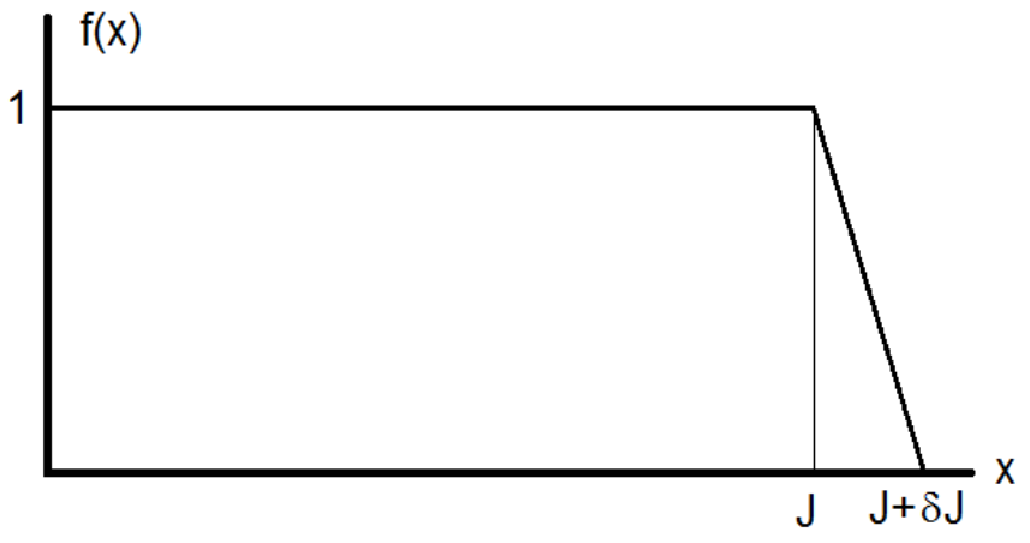
The dilatation operator can not arrange that the number of $Z$s between two magnons becomes negative. Thus, any bounds on sums in the definition of our simple states enforcing this are respected. On the other hand, the dilatation operator allows boundary magnons to hop arbitrarily far beyond the open string endpoint. Bounds in the sums for simple states enforcing this are not respected. Replace these bounds enforced as the upper limit of a sum, by bounds enforced by the cut off function. From Figure 2 we see that the cut off function is defined using a parameter $\delta J$. We require that ${\delta J\over J}\to 0$ as $N\to\infty$, so that at large $N$ the difference between these eigenstates and the simple states $|q_{1}\rangle_{s}$ vanishes, as demonstrated in Appendix B. We also want to ensure that

$\displaystyle f(i)=f(i+1)+\epsilon\qquad\forall i$

(4.11)

with $\epsilon\to 0$ as $N\to\infty$. (4.11) is needed to ensure that we do indeed obtain an eigenstate. It is straight forward to choose a function $f(x)$ with the required properties. We could for example choose $\delta J$ to be of order $N^{{1\over 4}}$. Our large $N$ answers are not sensitive to the details of the cut off function $f(x)$. When $1/N$ corrections to the eigenstates are computed $f(x)$ may be more constrained and we may need to reconsider the precise form of the cut off function and how we implement the bounds.

It is now straight forward to verify that, at large $N$, we have

	$\displaystyle D|\psi(q_{1})\rangle$	$\displaystyle=$	$\displaystyle 2\times{g_{YM}^{2}\over 8\pi^{2}}\left(1+\left[1-{n\over N}\right]-\sqrt{1-{n\over N}}(q_{1}+q_{1}^{-1})\right)|\psi(q_{1})\rangle$		(4.12)
		$\displaystyle=$	$\displaystyle 2g^{2}\left(1+\left[1-{n\over N}\right]-\sqrt{1-{n\over N}}(q_{1}+q_{1}^{-1})\right)|\psi(q_{1})\rangle$		(4.13)

The analysis for the dual giant graviton of momentum $n$ leads to

	$\displaystyle D|\psi(q_{1})\rangle$	$\displaystyle=$	$\displaystyle 2\times{g_{YM}^{2}\over 8\pi^{2}}\left(1+\left[1+{n\over N}\right]-\sqrt{1+{n\over N}}(q_{1}+q_{1}^{-1})\right)|\psi(q_{1})\rangle$		(4.14)
		$\displaystyle=$	$\displaystyle 2g^{2}\left(1+\left[1+{n\over N}\right]-\sqrt{1+{n\over N}}(q_{1}+q_{1}^{-1})\right)|\psi(q_{1})\rangle$		(4.15)

The generalization to include more magnons is straight forward. We will simply consider increasingly complicated examples and for each simply quote the final results. The discussion is most easily carried out using the occupation notation. For example, the simple states corresponding to three magnons are

	$\displaystyle|q_{1},q_{2},q_{3}\rangle$	$\displaystyle=$	$\displaystyle\sum_{n_{3}=0}^{J-1}\sum_{n_{2}=0}^{n_{3}}\sum_{n_{1}=0}^{n_{2}}q_{1}^{n_{1}}q_{2}^{n_{2}}q_{3}^{n_{3}}|G(n+J+n_{1}-n_{3});\{(n_{2}-n_{1}),(n_{3}-n_{2})\}\rangle$		(4.16)
		$\displaystyle+$	$\displaystyle\sum_{n_{1}=0}^{J-1}\sum_{n_{3}=0}^{n_{1}}\sum_{n_{2}=0}^{n_{3}}q_{1}^{n_{1}}q_{2}^{n_{2}}q_{3}^{n_{3}}|G(n+n_{1}-n_{3});\{(J+n_{2}-n_{1}),(n_{3}-n_{2})\}\rangle$		(4.17)
		$\displaystyle+$	$\displaystyle\sum_{n_{2}=0}^{J-1}\sum_{n_{1}=0}^{n_{2}}\sum_{n_{3}=0}^{n_{1}}q_{1}^{n_{1}}q_{2}^{n_{2}}q_{3}^{n_{3}}|G(n+n_{1}-n_{3});\{(n_{2}-n_{1}),(J+n_{3}-n_{2})\}\rangle$		(4.18)

where we have again lumped together the Young diagram labels $G(x)=R,R_{1}^{1},R_{2}^{1}=1^{x+1},1^{x},1^{x}$. The coefficient of the ket $|G(n+J-a-b);\{(a),(b)\}\rangle$ is given by the sum

$\displaystyle\sum_{n_{1}=0}^{J-1}(q_{1}q_{2}q_{3})^{n_{1}}q_{2}^{a}q_{3}^{a+b}$

(4.20)

which vanishes if $k_{1}+k_{2}+k_{3}\neq 0$. Consequently we can set $q_{3}=q_{1}^{-1}q_{2}^{-1}$. Including the cut off function, our energy eigenstates are given by

			$\displaystyle|\psi(q_{1},q_{2})\rangle=\sum_{n_{3}=0}^{\infty}\sum_{n_{2}=0}^{n_{3}}\sum_{n_{1}=0}^{n_{2}}q_{1}^{n_{1}-n_{3}}q_{2}^{n_{2}-n_{3}}f(n_{3})|G(n+J+n_{1}-n_{3});\{(n_{2}-n_{1}),(n_{3}-n_{2})\}\rangle$		(4.21)
		$\displaystyle+$	$\displaystyle\sum_{n_{1}=0}^{J+n_{2}}\sum_{n_{3}=0}^{\infty}\sum_{n_{2}=0}^{n_{3}}q_{1}^{n_{1}-n_{3}}q_{2}^{n_{2}-n_{3}}f(n_{1})f(J+n_{3}-n_{1})|G(n+n_{1}-n_{3});\{(J+n_{2}-n_{1}),(n_{3}-n_{2})\}\rangle$		(4.22)
		$\displaystyle+$	$\displaystyle\sum_{n_{2}=0}^{J+n_{3}}\sum_{n_{1}=0}^{n_{2}}\sum_{n_{3}=0}^{\infty}q_{1}^{n_{1}-n_{3}}q_{2}^{n_{2}-n_{3}}f(n_{2})f(J+n_{3}-n_{1})|G(n+n_{1}-n_{3});\{(n_{2}-n_{1}),(J+n_{3}-n_{2})\}\rangle$

It is a simple matter to see that

$\displaystyle D|\psi(q_{1},q_{2})\rangle=(E_{1}+E_{2}+E_{3})|\psi(q_{1},q_{2})\rangle$

(4.23)

where

	$\displaystyle E_{1}$	$\displaystyle=$	$\displaystyle g^{2}\left(1+\left[1-{n\over N}\right]-\sqrt{1-{n\over N}}(q_{1}+q_{1}^{-1})\right)$		(4.24)
	$\displaystyle E_{2}$	$\displaystyle=$	$\displaystyle g^{2}\left(2-q_{2}-q_{2}^{-1}\right)$		(4.25)
	$\displaystyle E_{3}$	$\displaystyle=$	$\displaystyle g^{2}\left(1+\left[1-{n\over N}\right]-\sqrt{1-{n\over N}}(q_{3}+q_{3}^{-1})\right)$		(4.26)

Now consider the extension to states containing many magnons: For an $M$ magnon state, consider all $M$ cyclic orderings of the “magnon positions”

	$\displaystyle n_{1}\leq n_{2}\leq n_{3}\leq\cdots\leq n_{M-2}\leq n_{M-1}\leq n_{M}\leq J-1$		(4.27)
	$\displaystyle n_{M}\leq n_{1}\leq n_{2}\leq n_{3}\leq\cdots\leq n_{M-2}\leq n_{M-1}\leq J-1$		(4.28)
	$\displaystyle n_{M-1}\leq n_{M}\leq n_{1}\leq n_{2}\leq n_{3}\leq\cdots\leq n_{M-2}\leq J-1$		(4.29)
	$\displaystyle\vdots\qquad\qquad\vdots\qquad\qquad\vdots$		(4.30)
	$\displaystyle n_{2}\leq n_{3}\leq\cdots\leq n_{M-2}\leq n_{M-1}\leq n_{M}\leq n_{1}\leq J-1$		(4.31)

Construct the differences $\{n_{2}-n_{1},n_{3}-n_{2},n_{4}-n_{3},\cdots,n_{M}-n_{M-1},n_{1}-n_{M}\}$. Every difference except for one is positive. Add $J$ to the difference that is negative, i.e. the resulting differences are $\{\Delta_{2},\Delta_{3},\Delta_{4},\cdots,\Delta_{M},\Delta_{1}\}$ with

$\displaystyle\begin{matrix}\cr\Delta_{i}\cr\cr\end{matrix}=\left\{\begin{matrix}n_{i}-n_{i-1}&{\rm if\quad}n_{i}\geq n_{i-1}\cr\cr J+n_{i}-n_{i-1}&{\rm if\quad}n_{i}\leq n_{i-1}\cr\end{matrix}\right.$

(4.32)

For each ordering in (4.31) we have a term in the simple state. This term is obtained by summing over all values of $\{n_{1},n_{2},\cdots,n_{L}\}$ consistent with the ordering considered, of the following summand

$\displaystyle q_{1}^{n_{1}}q_{2}^{n_{2}}\cdots q_{L}^{n_{M}}|1^{n+\Delta_{1}+1},1^{n+\Delta_{1}},1^{n+\Delta_{1}};\{(\Delta_{2}),(\Delta_{3}),\cdots,(\Delta_{M})\}\rangle$

(4.33)

Repeating the argument we outlined above, this term vanishes unless $q_{M}^{-1}=q_{1}q_{2}\cdots q_{M-1}$ so that the summand can be replaced by

$\displaystyle q_{1}^{n_{1}-n_{M}}q_{2}^{n_{2}-n_{M}}\cdots q_{M-1}^{n_{M-1}-n_{M}}|1^{n+\Delta_{1}+1},1^{n+\Delta_{1}},1^{n+\Delta_{1}};\{(\Delta_{2}),(\Delta_{3}),\cdots,(\Delta_{M})\}\rangle$

(4.34)

Finally, consider the extension to many string states and an arbitrary system of giant graviton branes. Each open string word is constructed as explained above. We add extra columns (one for each giant graviton) and rows (one for each dual giant graviton) to $R$. The labels $R^{k}_{1}$ and $R^{k}_{2}$ specify how the open strings are connected to the giant and dual giant gravitons. When describing twisted string states, the strings describe a closed loop, “punctuated by” the giant gravitons on which they end. As an example, consider a two giant graviton state, with a pair of strings stretching between the giant gravitons. The two strings carry a total momentum of $J$. Notice that we are using the two strings to define a single lattice of $J$ sites. One might have thought that the two strings would each define an independent lattice. To understand why we use the two strings to define a single lattice, recall that we are identifying the zero lattice momentum constraint with the constraint that the $su(2|2)$ central charges of the complete magnon state must vanish. There is a single $su(2|2)$ constraint on the two string state, not one constraint for each string. We interpret this as implying there is a single zero lattice momentum constraint for the two strings, and hence there is a single lattice for the two strings. This provides a straight forward way to satisfy the $su(2|2)$ central charge constraints. The first giant graviton has a momentum of $b_{0}$ and the second a momentum of $b_{1}$. The first string is excited by $M$ magnons with locations $\{n_{1},n_{2},\cdots,n_{M-1},n_{M}\}$ and the second by $\tilde{M}$ magnons with locations $\{\tilde{n}_{1},\tilde{n}_{2},\cdots,\tilde{n}_{\tilde{M}-1},\tilde{n}_{\tilde{M}}\}$ where we have switched to the lattice notation. We need to consider the $M+\tilde{M}$ orderings of the $\{n_{i}\}$ and $\{\tilde{n}_{i}\}$. Given a specific pair of orderings, we can again form the differences

	$\displaystyle\Delta_{1}$	$\displaystyle=$	$\displaystyle\left\{\begin{matrix}n_{1}-\tilde{n}_{M}&{\rm if\quad}n_{1}\geq\tilde{n}_{M}&\cr J+n_{1}-\tilde{n}_{M}&{\rm if\quad}n_{1}\leq\tilde{n}_{M}&\cr\end{matrix}\right.$		(4.35)
	$\displaystyle\begin{matrix}\cr\Delta_{i}\cr\cr\end{matrix}$	$\displaystyle=$	$\displaystyle\left\{\begin{matrix}n_{i}-n_{i-1}&{\rm if\quad}n_{i}\geq n_{i-1}&\cr&&i=2,3,\cdots,M\cr J+n_{i}-n_{i-1}&{\rm if\quad}n_{i}\leq n_{i-1}&\cr\end{matrix}\right.$		(4.36)
	$\displaystyle\Delta_{M+1}$	$\displaystyle=$	$\displaystyle\left\{\begin{matrix}\tilde{n}_{1}-n_{M}&{\rm if\quad}n_{M}\leq\tilde{n}_{1}&\cr J+\tilde{n}_{1}-n_{M}&{\rm if\quad}n_{M}\geq\tilde{n}_{1}&\cr\end{matrix}\right.$		(4.38)
	$\displaystyle\begin{matrix}\cr\Delta_{M+i}\cr\cr\end{matrix}$	$\displaystyle=$	$\displaystyle\left\{\begin{matrix}\tilde{n}_{i}-\tilde{n}_{i-1}&{\rm if\quad}\tilde{n}_{i}\geq\tilde{n}_{i-1}&\cr&&i=2,3,\cdots,\tilde{M}\cr J+\tilde{n}_{i}-\tilde{n}_{i-1}&{\rm if\quad}\tilde{n}_{i}\leq\tilde{n}_{i-1}&\cr\end{matrix}\right.$		(4.40)

For each ordering we again have a term in the simple state, obtained by summing over all values of $\{n_{1},n_{2},\cdots,n_{M},\tilde{n}_{1},\tilde{n}_{2},\cdots,\tilde{n}_{\tilde{M}}\}$ consistent with the ordering considered, of the following summand

$\displaystyle q_{1}^{n_{1}}\cdots q_{M}^{n_{M}}\tilde{q}_{1}^{\tilde{n}_{1}}\cdots\tilde{q}_{\tilde{M}}^{\tilde{n}_{\tilde{M}}}|G(\Delta_{1},\Delta_{M+1});\{(\Delta_{2}),(\Delta_{3}),\cdots,(\Delta_{M})\},\{(\Delta_{M+2}),(\Delta_{M+3}),\cdots,(\Delta_{M+\tilde{M}})\}\rangle$

(4.41)

where

$\displaystyle G(x,y)\equiv{\tiny\hbox{}\hskip 0.0pt{\vbox{\vbox{\hrule height=0.3pt\hbox{\vrule height=3.0589pt,width=0.3pt,depth=1.3595pt\hbox to3.3988pt{\hfil}\vrule height=3.0589pt,width=0.3pt,depth=1.3595pt\hbox to3.3988pt{\hfil}\vrule height=3.0589pt,width=0.3pt,depth=1.3595pt}\hrule height=0.3pt}\vskip-0.3pt\vbox{\hrule height=0.3pt\hbox{\vrule height=3.0589pt,width=0.3pt,depth=1.3595pt\hbox to3.3988pt{\hfil}\vrule height=3.0589pt,width=0.3pt,depth=1.3595pt\hbox to3.3988pt{\hfil}\vrule height=3.0589pt,width=0.3pt,depth=1.3595pt}\hrule height=0.3pt}\vskip-0.3pt\vbox{\hrule height=0.3pt\hbox{\vrule height=3.0589pt,width=0.3pt,depth=1.3595pt\hbox to3.3988pt{\hfil}\vrule height=3.0589pt,width=0.3pt,depth=1.3595pt\hbox to3.3988pt{\hfil}\vrule height=3.0589pt,width=0.3pt,depth=1.3595pt}\hrule height=0.3pt}\vskip-0.3pt\vbox{\hrule height=0.3pt\hbox{\vrule height=3.0589pt,width=0.3pt,depth=1.3595pt\hbox to3.3988pt{\hfil}\vrule height=3.0589pt,width=0.3pt,depth=1.3595pt\hbox to3.3988pt{\hfil}\vrule height=3.0589pt,width=0.3pt,depth=1.3595pt}\hrule height=0.3pt}\vskip-0.3pt\vbox{\hrule height=0.3pt\hbox{\vrule height=3.0589pt,width=0.3pt,depth=1.3595pt\hbox to3.3988pt{\hfil}\vrule height=3.0589pt,width=0.3pt,depth=1.3595pt\hbox to3.3988pt{\hfil}\vrule height=3.0589pt,width=0.3pt,depth=1.3595pt}\hrule height=0.3pt}\vskip-0.3pt\vbox{\hrule height=0.3pt\hbox{\vrule height=3.0589pt,width=0.3pt,depth=1.3595pt\hbox to3.3988pt{\hfil}\vrule height=3.0589pt,width=0.3pt,depth=1.3595pt\hbox to3.3988pt{\hfil}\vrule height=3.0589pt,width=0.3pt,depth=1.3595pt}\hrule height=0.3pt}\vskip-0.3pt\vbox{\hrule height=0.3pt\hbox{\vrule height=3.0589pt,width=0.3pt,depth=1.3595pt\hbox to3.3988pt{\hfil}\vrule height=3.0589pt,width=0.3pt,depth=1.3595pt\hbox to3.3988pt{\hfil}\vrule height=3.0589pt,width=0.3pt,depth=1.3595pt}\hrule height=0.3pt}\vskip-0.3pt\vbox{\hrule height=0.3pt\hbox{\vrule height=3.0589pt,width=0.3pt,depth=1.3595pt\hbox to3.3988pt{\hfil}\vrule height=3.0589pt,width=0.3pt,depth=1.3595pt}\hrule height=0.3pt}\vskip-0.3pt\vbox{\hrule height=0.3pt\hbox{\vrule height=3.0589pt,width=0.3pt,depth=1.3595pt\hbox to3.3988pt{\hfil}\vrule height=3.0589pt,width=0.3pt,depth=1.3595pt}\hrule height=0.3pt}\vskip-0.3pt\vbox{\hrule height=0.3pt\hbox{\vrule height=3.0589pt,width=0.3pt,depth=1.3595pt\hbox to3.3988pt{\hfil}\vrule height=3.0589pt,width=0.3pt,depth=1.3595pt}\hrule height=0.3pt}\vskip-0.3pt\vbox{\hrule height=0.3pt\hbox{\vrule height=3.0589pt,width=0.3pt,depth=1.3595pt\hbox to3.3988pt{\hfil}\vrule height=3.0589pt,width=0.3pt,depth=1.3595pt}\hrule height=0.3pt}\vskip-0.3pt\vbox{\hrule height=0.3pt\hbox{\vrule height=3.0589pt,width=0.3pt,depth=1.3595pt\hbox to3.3988pt{\hfil}\vrule height=3.0589pt,width=0.3pt,depth=1.3595pt}\hrule height=0.3pt}\vskip-0.3pt}}\hskip 0.0pt,\hbox{}\hskip 0.0pt{\vbox{\vbox{\hrule height=0.3pt\hbox{\vrule height=3.0589pt,width=0.3pt,depth=1.3595pt\hbox to3.3988pt{\hfil$\,$\hfil}\vrule height=3.0589pt,width=0.3pt,depth=1.3595pt\hbox to3.3988pt{\hfil$\,$\hfil}\vrule height=3.0589pt,width=0.3pt,depth=1.3595pt}\hrule height=0.3pt}\vskip-0.3pt\vbox{\hrule height=0.3pt\hbox{\vrule height=3.0589pt,width=0.3pt,depth=1.3595pt\hbox to3.3988pt{\hfil$\,$\hfil}\vrule height=3.0589pt,width=0.3pt,depth=1.3595pt\hbox to3.3988pt{\hfil$\,$\hfil}\vrule height=3.0589pt,width=0.3pt,depth=1.3595pt}\hrule height=0.3pt}\vskip-0.3pt\vbox{\hrule height=0.3pt\hbox{\vrule height=3.0589pt,width=0.3pt,depth=1.3595pt\hbox to3.3988pt{\hfil$\,$\hfil}\vrule height=3.0589pt,width=0.3pt,depth=1.3595pt\hbox to3.3988pt{\hfil$\,$\hfil}\vrule height=3.0589pt,width=0.3pt,depth=1.3595pt}\hrule height=0.3pt}\vskip-0.3pt\vbox{\hrule height=0.3pt\hbox{\vrule height=3.0589pt,width=0.3pt,depth=1.3595pt\hbox to3.3988pt{\hfil$\,$\hfil}\vrule height=3.0589pt,width=0.3pt,depth=1.3595pt\hbox to3.3988pt{\hfil$\,$\hfil}\vrule height=3.0589pt,width=0.3pt,depth=1.3595pt}\hrule height=0.3pt}\vskip-0.3pt\vbox{\hrule height=0.3pt\hbox{\vrule height=3.0589pt,width=0.3pt,depth=1.3595pt\hbox to3.3988pt{\hfil$\,$\hfil}\vrule height=3.0589pt,width=0.3pt,depth=1.3595pt\hbox to3.3988pt{\hfil$\,$\hfil}\vrule height=3.0589pt,width=0.3pt,depth=1.3595pt}\hrule height=0.3pt}\vskip-0.3pt\vbox{\hrule height=0.3pt\hbox{\vrule height=3.0589pt,width=0.3pt,depth=1.3595pt\hbox to3.3988pt{\hfil$\,$\hfil}\vrule height=3.0589pt,width=0.3pt,depth=1.3595pt\hbox to3.3988pt{\hfil$\,$\hfil}\vrule height=3.0589pt,width=0.3pt,depth=1.3595pt}\hrule height=0.3pt}\vskip-0.3pt\vbox{\hrule height=0.3pt\hbox{\vrule height=3.0589pt,width=0.3pt,depth=1.3595pt\hbox to3.3988pt{\hfil$\,$\hfil}\vrule height=3.0589pt,width=0.3pt,depth=1.3595pt\hbox to3.3988pt{\hfil$2$\hfil}\vrule height=3.0589pt,width=0.3pt,depth=1.3595pt}\hrule height=0.3pt}\vskip-0.3pt\vbox{\hrule height=0.3pt\hbox{\vrule height=3.0589pt,width=0.3pt,depth=1.3595pt\hbox to3.3988pt{\hfil$\,$\hfil}\vrule height=3.0589pt,width=0.3pt,depth=1.3595pt}\hrule height=0.3pt}\vskip-0.3pt\vbox{\hrule height=0.3pt\hbox{\vrule height=3.0589pt,width=0.3pt,depth=1.3595pt\hbox to3.3988pt{\hfil$\,$\hfil}\vrule height=3.0589pt,width=0.3pt,depth=1.3595pt}\hrule height=0.3pt}\vskip-0.3pt\vbox{\hrule height=0.3pt\hbox{\vrule height=3.0589pt,width=0.3pt,depth=1.3595pt\hbox to3.3988pt{\hfil$\,$\hfil}\vrule height=3.0589pt,width=0.3pt,depth=1.3595pt}\hrule height=0.3pt}\vskip-0.3pt\vbox{\hrule height=0.3pt\hbox{\vrule height=3.0589pt,width=0.3pt,depth=1.3595pt\hbox to3.3988pt{\hfil$\,$\hfil}\vrule height=3.0589pt,width=0.3pt,depth=1.3595pt}\hrule height=0.3pt}\vskip-0.3pt\vbox{\hrule height=0.3pt\hbox{\vrule height=3.0589pt,width=0.3pt,depth=1.3595pt\hbox to3.3988pt{\hfil$1$\hfil}\vrule height=3.0589pt,width=0.3pt,depth=1.3595pt}\hrule height=0.3pt}\vskip-0.3pt}}\hskip 0.0pt,\hbox{}\hskip 0.0pt{\vbox{\vbox{\hrule height=0.3pt\hbox{\vrule height=3.0589pt,width=0.3pt,depth=1.3595pt\hbox to3.3988pt{\hfil$\,$\hfil}\vrule height=3.0589pt,width=0.3pt,depth=1.3595pt\hbox to3.3988pt{\hfil$\,$\hfil}\vrule height=3.0589pt,width=0.3pt,depth=1.3595pt}\hrule height=0.3pt}\vskip-0.3pt\vbox{\hrule height=0.3pt\hbox{\vrule height=3.0589pt,width=0.3pt,depth=1.3595pt\hbox to3.3988pt{\hfil$\,$\hfil}\vrule height=3.0589pt,width=0.3pt,depth=1.3595pt\hbox to3.3988pt{\hfil$\,$\hfil}\vrule height=3.0589pt,width=0.3pt,depth=1.3595pt}\hrule height=0.3pt}\vskip-0.3pt\vbox{\hrule height=0.3pt\hbox{\vrule height=3.0589pt,width=0.3pt,depth=1.3595pt\hbox to3.3988pt{\hfil$\,$\hfil}\vrule height=3.0589pt,width=0.3pt,depth=1.3595pt\hbox to3.3988pt{\hfil$\,$\hfil}\vrule height=3.0589pt,width=0.3pt,depth=1.3595pt}\hrule height=0.3pt}\vskip-0.3pt\vbox{\hrule height=0.3pt\hbox{\vrule height=3.0589pt,width=0.3pt,depth=1.3595pt\hbox to3.3988pt{\hfil$\,$\hfil}\vrule height=3.0589pt,width=0.3pt,depth=1.3595pt\hbox to3.3988pt{\hfil$\,$\hfil}\vrule height=3.0589pt,width=0.3pt,depth=1.3595pt}\hrule height=0.3pt}\vskip-0.3pt\vbox{\hrule height=0.3pt\hbox{\vrule height=3.0589pt,width=0.3pt,depth=1.3595pt\hbox to3.3988pt{\hfil$\,$\hfil}\vrule height=3.0589pt,width=0.3pt,depth=1.3595pt\hbox to3.3988pt{\hfil$\,$\hfil}\vrule height=3.0589pt,width=0.3pt,depth=1.3595pt}\hrule height=0.3pt}\vskip-0.3pt\vbox{\hrule height=0.3pt\hbox{\vrule height=3.0589pt,width=0.3pt,depth=1.3595pt\hbox to3.3988pt{\hfil$\,$\hfil}\vrule height=3.0589pt,width=0.3pt,depth=1.3595pt\hbox to3.3988pt{\hfil$\,$\hfil}\vrule height=3.0589pt,width=0.3pt,depth=1.3595pt}\hrule height=0.3pt}\vskip-0.3pt\vbox{\hrule height=0.3pt\hbox{\vrule height=3.0589pt,width=0.3pt,depth=1.3595pt\hbox to3.3988pt{\hfil$\,$\hfil}\vrule height=3.0589pt,width=0.3pt,depth=1.3595pt\hbox to3.3988pt{\hfil$1$\hfil}\vrule height=3.0589pt,width=0.3pt,depth=1.3595pt}\hrule height=0.3pt}\vskip-0.3pt\vbox{\hrule height=0.3pt\hbox{\vrule height=3.0589pt,width=0.3pt,depth=1.3595pt\hbox to3.3988pt{\hfil$\,$\hfil}\vrule height=3.0589pt,width=0.3pt,depth=1.3595pt}\hrule height=0.3pt}\vskip-0.3pt\vbox{\hrule height=0.3pt\hbox{\vrule height=3.0589pt,width=0.3pt,depth=1.3595pt\hbox to3.3988pt{\hfil$\,$\hfil}\vrule height=3.0589pt,width=0.3pt,depth=1.3595pt}\hrule height=0.3pt}\vskip-0.3pt\vbox{\hrule height=0.3pt\hbox{\vrule height=3.0589pt,width=0.3pt,depth=1.3595pt\hbox to3.3988pt{\hfil$\,$\hfil}\vrule height=3.0589pt,width=0.3pt,depth=1.3595pt}\hrule height=0.3pt}\vskip-0.3pt\vbox{\hrule height=0.3pt\hbox{\vrule height=3.0589pt,width=0.3pt,depth=1.3595pt\hbox to3.3988pt{\hfil$\,$\hfil}\vrule height=3.0589pt,width=0.3pt,depth=1.3595pt}\hrule height=0.3pt}\vskip-0.3pt\vbox{\hrule height=0.3pt\hbox{\vrule height=3.0589pt,width=0.3pt,depth=1.3595pt\hbox to3.3988pt{\hfil$2$\hfil}\vrule height=3.0589pt,width=0.3pt,depth=1.3595pt}\hrule height=0.3pt}\vskip-0.3pt}}\hskip 0.0pt}$

(4.43)

In the first Young diagram above there are $b_{1}+y+1$ rows with 2 boxes in each row and $b_{0}+x-b_{1}-y-1$ rows with 1 box in each row. Repeating the argument we outlined above, this term vanishes unless $\tilde{q}_{\tilde{M}}^{-1}=q_{1}\cdots q_{M}\tilde{q}_{1}\cdots\tilde{q}_{\tilde{M}-1}$ so that the summand can be replaced by

$\displaystyle q_{1}^{n_{1}-\tilde{n}_{\tilde{M}}}q_{2}^{n_{2}-\tilde{n}_{\tilde{M}}}\cdots\tilde{q}_{\tilde{M}-1}^{\tilde{n}_{\tilde{M}-1}-\tilde{n}_{\tilde{M}}}|G(\Delta_{1},\Delta_{M+1});\{(\Delta_{2}),(\Delta_{3}),\cdots,(\Delta_{M})\},\{(\Delta_{M+2}),(\Delta_{M+3}),\cdots,(\Delta_{M+\tilde{M}})\}\rangle$

(4.44)

This completes our discussion of the large $N$ asymptotic eigenstates. We will now consider the dual string theory description of these states.

References

- [1] D. E. Berenstein, J. M. Maldacena and H. S. Nastase, “Strings in flat space and pp waves from N=4 superYang-Mills,” JHEP 0204, 013 (2002) [hep-th/0202021].
- [2] N. Beisert, C. Ahn, L. F. Alday, Z. Bajnok, J. M. Drummond, L. Freyhult, N. Gromov and R. A. Janik et al., “Review of AdS/CFT Integrability: An Overview,” Lett. Math. Phys. 99, 3 (2012) [arXiv:1012.3982 [hep-th]].
- [3] N. Beisert, “The SU(2—2) dynamic S-matrix,” Adv. Theor. Math. Phys. 12, 945 (2008) [hep-th/0511082].
- [4] N. Beisert, “The Analytic Bethe Ansatz for a Chain with Centrally Extended su(2—2) Symmetry,” J. Stat. Mech. 0701, P01017 (2007) [nlin/0610017 [nlin.SI]].
- [5] D. M. Hofman and J. M. Maldacena, “Reflecting magnons,” JHEP 0711, 063 (2007) [arXiv:0708.2272 [hep-th]].
- [6] D. Berenstein, D. H. Correa and S. E. Vazquez, “All loop BMN state energies from matrices,” JHEP 0602, 048 (2006) [hep-th/0509015].
- [7] D. M. Hofman and J. M. Maldacena, “Giant Magnons,” J. Phys. A 39, 13095 (2006) [hep-th/0604135].
- [8] D. Berenstein, “A Toy model for the AdS / CFT correspondence,” JHEP 0407, 018 (2004) [hep-th/0403110].
- [9] H. Lin, O. Lunin and J. M. Maldacena, “Bubbling AdS space and 1/2 BPS geometries,” JHEP 0410, 025 (2004) [hep-th/0409174].
- [10] V. Balasubramanian, M. Berkooz, A. Naqvi and M. J. Strassler, “Giant gravitons in conformal field theory,” JHEP 0204, 034 (2002) [hep-th/0107119].
- [11] S. Corley, A. Jevicki and S. Ramgoolam, “Exact correlators of giant gravitons from dual N=4 SYM theory,” Adv. Theor. Math. Phys. 5, 809 (2002) [hep-th/0111222].
- [12] S. Corley and S. Ramgoolam, “Finite factorization equations and sum rules for BPS correlators in N=4 SYM theory,” Nucl. Phys. B 641, 131 (2002) [hep-th/0205221].
- [13] T. W. Brown, P. J. Heslop and S. Ramgoolam, “Diagonal multi-matrix correlators and BPS operators in N=4 SYM,” JHEP 0802, 030 (2008) [arXiv:0711.0176 [hep-th]].
- [14] T. W. Brown, P. J. Heslop and S. Ramgoolam, “Diagonal free field matrix correlators, global symmetries and giant gravitons,” JHEP 0904, 089 (2009) [arXiv:0806.1911 [hep-th]].
- [15] Y. Kimura and S. Ramgoolam, “Branes, anti-branes and brauer algebras in gauge-gravity duality,” JHEP 0711, 078 (2007) [arXiv:0709.2158 [hep-th]].
- [16] Y. Kimura and S. Ramgoolam, “Enhanced symmetries of gauge theory and resolving the spectrum of local operators,” Phys. Rev. D 78, 126003 (2008) [arXiv:0807.3696 [hep-th]].
- [17] Y. Kimura, “Non-holomorphic multi-matrix gauge invariant operators based on Brauer algebra,” JHEP 0912, 044 (2009) [arXiv:0910.2170 [hep-th]].
- [18] Y. Kimura, S. Ramgoolam and D. Turton, “Free particles from Brauer algebras in complex matrix models,” JHEP 1005, 052 (2010) [arXiv:0911.4408 [hep-th]].
- [19] Y. Kimura, “Quarter BPS classified by Brauer algebra,” JHEP 1005, 103 (2010) [arXiv:1002.2424 [hep-th]].
- [20] Y. Kimura and H. Lin, “Young diagrams, Brauer algebras, and bubbling geometries,” JHEP 1201, 121 (2012) [arXiv:1109.2585 [hep-th]].
- [21] Y. Kimura, “Correlation functions and representation bases in free N=4 Super Yang-Mills,” Nucl. Phys. B 865, 568 (2012) [arXiv:1206.4844 [hep-th]].
- [22] Y. Kimura, “Non-planar operator mixing by Brauer representations,” Nucl. Phys. B 875, 790 (2013) [arXiv:1302.6404 [hep-th]].
- [23] V. Balasubramanian, D. Berenstein, B. Feng and M. x. Huang, “D-branes in Yang-Mills theory and emergent gauge symmetry,” JHEP 0503, 006 (2005) [hep-th/0411205].
- [24] R. de Mello Koch, J. Smolic and M. Smolic, “Giant Gravitons - with Strings Attached (I),” JHEP 0706, 074 (2007) [hep-th/0701066].
- [25] R. de Mello Koch, J. Smolic and M. Smolic, “Giant Gravitons - with Strings Attached (II),” JHEP 0709, 049 (2007) [hep-th/0701067].
- [26] D. Bekker, R. de Mello Koch and M. Stephanou, “Giant Gravitons - with Strings Attached. III.,” JHEP 0802, 029 (2008) [arXiv:0710.5372 [hep-th]].
- [27] R. Bhattacharyya, S. Collins and R. d. M. Koch, “Exact Multi-Matrix Correlators,” JHEP 0803, 044 (2008) [arXiv:0801.2061 [hep-th]].
- [28] R. Bhattacharyya, R. de Mello Koch and M. Stephanou, “Exact Multi-Restricted Schur Polynomial Correlators,” JHEP 0806, 101 (2008) [arXiv:0805.3025 [hep-th]].
- [29] R. d. M. Koch, G. Mashile and N. Park, “Emergent Threebrane Lattices,” Phys. Rev. D 81, 106009 (2010) [arXiv:1004.1108 [hep-th]].
- [30] V. De Comarmond, R. de Mello Koch and K. Jefferies, “Surprisingly Simple Spectra,” JHEP 1102, 006 (2011) [arXiv:1012.3884 [hep-th]].
- [31] W. Carlson, R. d. M. Koch and H. Lin, “Nonplanar Integrability,” JHEP 1103, 105 (2011) [arXiv:1101.5404 [hep-th]].
- [32] R. d. M. Koch, M. Dessein, D. Giataganas and C. Mathwin, “Giant Graviton Oscillators,” JHEP 1110, 009 (2011) [arXiv:1108.2761 [hep-th]].
- [33] R. de Mello Koch and S. Ramgoolam, “A double coset ansatz for integrability in AdS/CFT,” JHEP 1206, 083 (2012) [arXiv:1204.2153 [hep-th]].
- [34] R. de Mello Koch, G. Kemp and S. Smith, “From Large N Nonplanar Anomalous Dimensions to Open Spring Theory,” Phys. Lett. B 711, 398 (2012) [arXiv:1111.1058 [hep-th]].
- [35] P. Caputa, R. de Mello Koch and P. Diaz, “A basis for large operators in N=4 SYM with orthogonal gauge group,” JHEP 1303, 041 (2013) [arXiv:1301.1560 [hep-th]].
- [36] P. Caputa, R. d. M. Koch and P. Diaz, “Operators, Correlators and Free Fermions for SO(N) and Sp(N),” JHEP 1306, 018 (2013) [arXiv:1303.7252 [hep-th]].
- [37] P. Diaz, “Orthogonal Schurs for Classical Gauge Groups,” JHEP 1310, 228 (2013) [arXiv:1309.1180 [hep-th]].
- [38] G. Kemp, “SO(N) restricted Schur polynomials,” J. Math. Phys. 56, no. 2, 022302 (2015) [arXiv:1405.7017 [hep-th]].
- [39] G. Kemp, “Restricted Schurs and correlators for and ,” JHEP 1408, 137 (2014) [arXiv:1406.3854 [hep-th]].
- [40] P. Diaz, “Novel charges in CFT‘s,” JHEP 1409, 031 (2014) [arXiv:1406.7671 [hep-th]].
- [41] D. Berenstein, “Giant gravitons: a collective coordinate approach,” Phys. Rev. D 87, no. 12, 126009 (2013) [arXiv:1301.3519 [hep-th]].
- [42] D. Berenstein and E. Dzienkowski, “Open spin chains for giant gravitons and relativity,” JHEP 1308, 047 (2013) [arXiv:1305.2394 [hep-th]].
- [43] D. Berenstein, “Sketches of emergent geometry in the gauge/gravity duality,” Fortsch. Phys. 62, 776 (2014) [arXiv:1404.7052 [hep-th]].
- [44] D. Berenstein and E. Dzienkowski, “Giant gravitons and the emergence of geometric limits in beta-deformations of SYM,” JHEP 1501, 126 (2015) [arXiv:1408.3620 [hep-th]].
- [45] D. Berenstein, “On the central charge extension of the N=4 SYM spin chain,” arXiv:1411.5921 [hep-th].
- [46] Y. Kimura and R. Suzuki, arXiv:1503.06210 [hep-th].
- [47] V. Balasubramanian, M. x. Huang, T. S. Levi and A. Naqvi, “Open strings from N=4 superYang-Mills,” JHEP 0208, 037 (2002) [hep-th/0204196].
- [48] S. R. Das, A. Jevicki and S. D. Mathur, “Vibration modes of giant gravitons,” Phys. Rev. D 63, 024013 (2001) [hep-th/0009019].
- [49] O. Aharony, Y. E. Antebi, M. Berkooz and R. Fishman, “’Holey sheets’: Pfaffians and subdeterminants as D-brane operators in large N gauge theories,” JHEP 0212, 069 (2002) [hep-th/0211152].
- [50] D. Berenstein, “Shape and holography: Studies of dual operators to giant gravitons,” Nucl. Phys. B 675, 179 (2003) [hep-th/0306090].
- [51] D. Berenstein, D. H. Correa and S. E. Vazquez, “A Study of open strings ending on giant gravitons, spin chains and integrability,” JHEP 0609, 065 (2006) [hep-th/0604123].
- [52] D. Berenstein and S. E. Vazquez, “Integrable open spin chains from giant gravitons,” JHEP 0506, 059 (2005) [hep-th/0501078].
- [53] D. Berenstein, D. H. Correa and S. E. Vazquez, “Quantizing open spin chains with variable length: An Example from giant gravitons,” Phys. Rev. Lett. 95, 191601 (2005) [hep-th/0502172].
- [54] D. Garner, S. Ramgoolam and C. Wen, “Thresholds of large N factorization in CFT4: exploring bulk spacetime in AdS5,” JHEP 1411, 076 (2014) [arXiv:1403.5281 [hep-th]].
- [55]
J. A. Minahan and K. Zarembo,
“The Bethe-ansatz for N = 4 super Yang-Mills,”
JHEP 0303, 013 (2003)
[arXiv:hep-th/0212208]
N. Beisert, C. Kristjansen and M. Staudacher, “The dilatation operator of N = 4 super Yang-Mills theory,” Nucl. Phys. B 664, 131 (2003) [arXiv:hep-th/0303060]. - [56] R. C. Myers, “Dielectric branes,” JHEP 9912, 022 (1999) doi:10.1088/1126-6708/1999/12/022 [hep-th/9910053].
- [57] J. McGreevy, L. Susskind and N. Toumbas, “Invasion of the giant gravitons from Anti-de Sitter space,” JHEP 0006, 008 (2000) [hep-th/0003075].
- [58] A. Hashimoto, S. Hirano and N. Itzhaki, “Large branes in AdS and their field theory dual,” JHEP 0008, 051 (2000) [hep-th/0008016].
- [59] M. T. Grisaru, R. C. Myers and O. Tafjord, “SUSY and goliath,” JHEP 0008, 040 (2000) [hep-th/0008015].
- [60] R. A. Janik, “The AdS(5) x S**5 superstring worldsheet S-matrix and crossing symmetry,” Phys. Rev. D 73, 086006 (2006) [hep-th/0603038].
- [61] D. H. Correa and C. A. S. Young, “Asymptotic Bethe equations for open boundaries in planar AdS/CFT,” J. Phys. A 43, 145401 (2010) doi:10.1088/1751-8113/43/14/145401 [arXiv:0912.0627 [hep-th]].
- [62] H. Lin, “Relation between large dimension operators and oscillator algebra of Young diagrams,” Int. J. Geom. Meth. Mod. Phys. 12, no. 04, 1550047 (2015) [arXiv:1407.7815 [hep-th]].
- [63] F. Denef, “Supergravity flows and D-brane stability,” JHEP 0008, 050 (2000) [hep-th/0005049].
- [64] M. Staudacher, “The Factorized S-matrix of CFT/AdS,” JHEP 0505, 054 (2005) [hep-th/0412188].
- [65] L. Freyhult, C. Kristjansen and T. Mansson, “Integrable spin chains with U(1)**3 symmetry and generalized Lunin-Maldacena backgrounds,” JHEP 0512, 008 (2005) [hep-th/0510221].