Electronic excitations in quasi-2D crystals: What theoretical quantities are relevant to experiment?
Abstract
The ab initio theory of electronic excitations in atomically thin [quasi-two-dimensional (Q2D)] crystals presents extra challenges in comparison to both the bulk and purely 2D cases. We argue that the conventionally used energy-loss function (where , , and are the dielectric function, the momentum, and the energy transfer, respectively) is not, generally speaking, the suitable quantity for the interpretation of the electron-energy loss spectroscopy (EELS) in the Q2D case, and we construct different functions pertinent to the EELS experiments on Q2D crystals. Secondly, we emphasize the importance and develop a convenient procedure of the elimination of the spurious inter-layer interaction inherent to the use of the 3D super-cell method for the calculation of excitations in Q2D crystals. Thirdly, we resolve the existing controversy in the interpretation of the so-called and excitations in monolayer graphene by demonstrating that both dispersive collective excitations (plasmons) and non-dispersive single-particle (inter-band) transitions fall in the same energy ranges, where they strongly influence each other.
1 Introduction
Quasi two-dimensional (Q2D) crystals (the systems periodic and infinite in two dimensions while of atomic-size thickness) are presently attracting much of attention because of their potential in future nano-technologies. In particular, the electronic excitations in Q2D crystals, such as electron-hole pairs generation, plasmons, excitons, etc., are of great importance, since they determine the response to external actions, and, ultimately, shape the materials’ functionality (see, e.g., [1] for a recent review). At the same time, the theoretical approaches as well as the computational methods to deal with the excitations in Q2D systems become much more involved compared to both the three-dimensional (3D) and purely 2D cases, and are still far from finally established.
Indeed, in both purely 3D and purely 2D cases (the latter referring to model systems of zero thickness), one usually introduces the dielectric function , where is the wave-vector of the corresponding dimensionality, and is the frequency. The definition of reads 11 1 In this paper we are concerned with the longitudinal fields.
| (1) |
where and are the externally applied and the total (external plus induced) scalar potentials of the electric field, respectively. The definition (1) is not, however, straightforwardly transferable to the Q2D case, which can be easily appreciated by considering that depends on the (perpendicular to the layer) coordinate, even when is uniform in direction. Therefore, we need to redefine the dielectric function (energy-loss function, conductivity, etc.) of a Q2D crystal in accordance to the system’s structure. Importantly, the new definitions must be consistent with the quantities measured experimentally, the violation of which requirement having caused much of confusion in recent literature.
Secondly, the widest used at this time method of dealing with Q2D systems numerically is the super-cell geometry approach. This is to artificially replicate the system periodically in direction, choosing the distance between the layers large enough to prevent the inter-layer interactions. The resulting fictitious system is 3D-periodic, and well developed 3D solid-state methods as well as the existing 3D software can be used to efficiently handle it. In the ground-state calculations, the interpretation of the super-cell results is straightforward: Provided that the inter-layer distance is such that the corresponding wave-functions do not overlap, properties of an isolated single layer coincide with those of a single super-cell.
However, if we are concerned with the dynamic response to electric field, the situation changes. In the case of a Q2D crystal, the electric field decays into vacuum as . Clearly, whatever large is the separation between the layers, at sufficiently small the inter-layer interaction persists, and results of the super-cell calculation cannot be literally transferred to a single layer. A simple method of taking very large does not work, because small -s are often of special interest, and the computational load grows rapidly with the increase of . Therefore, we need to establish relations between the response functions of the fictitious 3D array system and those of the single layer of interest. The paramount requirement to these relations (test for sanity) is that they should produce the same response functions of a single layer from the differing 3D response functions calculated with different separations .
In this paper, in the framework of the time-dependent density-functional theory (TDDFT), we construct a scheme satisfying the above requirements. As its practical application, we calculate and perform a detailed analysis of the excitation spectrum of a single-layer graphene in the 1-30 eV energy range. Resolving the recent controversy in the interpretation of the and peaks as plasmons [2, 3, 4, 5] or single-particle inter-band transitions [6], we show that, while the problem is far more complicated than thought before, there do exist prominent and plasmons in graphene, although they overlap with the inter-band transitions. The isolation of the both kinds of excitations becomes possible by following the wave-vector dependence of spectra (spatial dispersion). We also show that much of the previous confusion was due to using unsuitable theoretical quantities for comparison with experiment, as well as to the uncritical use of the results of the super-cell calculations in application to Q2D systems.
This paper is organized as follows. In Sec. 2 we re-examine and revise the definitions of the response-functions (dielectric function, energy-loss function, conductivity) pertinent to measurements on Q2D crystals. Sec. 3 is devoted to the methods of obtaining the response-functions of Q2D crystals from the 3D super-cell calculations. In Sec. 4 we present results of calculations performed for graphene as an important example of a Q2D crystal, discuss the differences arising from the use of our theory, and compare with experiment. Section 5 contains conclusions, and in the Appendix we give the derivation of some formulas presented in Sec. 3. We use the atomic units () unless explicitly specified otherwise.
2 Linear response of quasi-2D crystals: Definition of quantities
Quasi-2D crystals are neither periodic three-dimensionally nor strictly two-dimensional within the mathematical plane: They rather have a finite atomic or nano-scale thickness. Accordingly, one has to exercise caution in the choice of quantities (dielectric function, conductivity, density-response function, etc.) which characterize the dielectric response, giving them rigorous, suitable for Q2D systems, meaning. The safe way to do this is to start from the general 3D case without assuming the periodicity (translational invariance) in any direction. The density-response function is defined in the real-space representation as
| (2) |
where is the scalar potential of the externally applied electric field and is the charge-density induced in the system in response to . The inverse generalized dielectric function is defined as
| (3) |
where is the total (external plus induced) potential, and it is expressed through as
| (4) |
By Fourier-transform, Eqs. (2)-(4) can be equivalently written in the reciprocal-space representation, of which we will need only
| (5) |
For Q2D crystals, we will use the mixed reciprocal- and real-space representation, in the plane and direction, respectively. Then the definition (2) becomes
| (6) |
where and are the 2D reciprocal lattice vectors, and is the 2D wave-vector in the first Brillouin zone. We will also need the expression for the induced potential
| (7) |
We distinguish between different kinds of experimental setups, where it will be shown that the measurable quantities correspond to different definitions of the energy-loss function.
2.1 Electron energy-loss spectroscopy
The principal experimental method of probing - and -dependent response of Q2D systems is the Electron Energy-Loss Spectroscopy (EELS). We will consider separately the reflection and transmission EELS.
2.1.1 Reflection EELS.
In reflection EELS, the quantity, which characterizes the inelastic electron scattering, is the so-called -function [7]22 2 In this paper, we restrict ourselves to the dipole scattering regime [7]. Impact-scattering regime is more involved, requiring the solution of the inelastic scattering problem within the distorted-waves method [8, 9, 10], which is outside the scope of this paper.. Its definition reads: Let the external potential be33 3 Everywhere below, only the dependence of quantities is written down explicitly. The implied and dependence is always .
| (8) |
Then asymptotically at
| (9) |
With the use of Eqs. (6) and (7), the -function can be written as [11, 12, 7]
| (10) |
When and are substituted with the incident electron’s loss of the parallel momentum and energy, respectively, the differential cross-section of the inelastic electron scattering in the reflection geometry is determined by the energy-loss function , i.e.,
| (11) |
where is the element of the solid-angle of the detection of the scattered electron, , , , , and are the momenta of the incident and scattered electron, respectively. Equation (10) expresses through the density-response function .
2.1.2 Transmission EELS.
For the transmission EELS of an arbitrary (possibly, non-periodic) target, the differential cross-section of the inelastic electron scattering is proportional to the energy-loss function (see, e.g., [13])
| (12) |
We emphasize, that in the right-hand side of Eq. (12) of Eq. (5) enters with and both substituted with the same momentum transfer .
We consider the case of normal incidence. Then
| (13) |
| (14) |
and, since is large,
| (15) |
2.1.3 In-plane electronic transport.
Let us calculate the conductivity and the energy dissipation in a Q2D crystal under the action of the uniform in direction external potential
| (17) |
Then, by Eq. (6),
| (18) |
and for the 2D particle-density averaged in the plane
| (19) |
Using the continuity equation
| (20) |
where is the 2D current-density, we can write
| (21) |
and since, by Eq. (17), ,
| (22) |
where is the 2D conductivity with respect to the external field, which is given by
| (23) |
For the energy dissipation per unit time per unit cell area under the action of the external potential (17) we can write44 4 Because is the quadratic rather than linear property, we must temporarily return to the representation.
| (24) |
where and are well defined 3D current-density and electric field, respectively, and is the 2D unit cell of the Q2D crystal. Since carriers do not commit work on themselves, Eq. (24) can be rewritten as
| (25) |
and simplified to
| (26) | |||||
Using Eqs. (6) and (17), we can rewrite Eq. (26) as
| (27) |
The important conclusion of Sections 2.1.2 - 2.1.3 is that the energy losses in the reflection EELS, transmission EELS, and the energy dissipation in the in-plane transport are governed by the quantities , , and , respectively, which, for a Q2D crystal, are clearly different quantities. We note that in the limiting case of the purely 2D (zero-thickness) crystal, contains , and, consequently, all these three quantities coincide.
2.1.4 Dielectric function of Q2D crystal.
It has already been noted in Sec. 1 that the dielectric function cannot be rigorously introduced for a Q2D crystal in a simple multiplicative way via Eq. (1). This is, in the first place, due to the uncertainty at which must be used. It is, however, convenient to keep the notion of the dielectric function on the intuitive level, resorting to an analogy with the purely 2D system. In the latter case
| (28) |
where is the 2D density-response function and the relation holds
| (29) |
where is the dielectric function of the 2D system. By Eqs. (23) and (28)
| (30) |
and, using Eq. (29)
| (31) |
For a Q2D crystal, we define the dielectric function using Eq. (31), where in the right-hand side we substitute of Eq. (23), which is a well defined quantity for the Q2D crystal. Therefore
| (32) |
By comparing Eqs. (16), (10), and (32), we see that the inelastic scattering of electrons in EELS of Q2D system is not defined by the loss-function . It will be shown that this difference is of a quantitative importance in the interpretation of the measurements on Q2D crystals.
Below we will see that it is convenient to have our results in the full reciprocal-space representation. Using the Fourier expansion in the interval, where at this point we consider an arbitrary sufficiently large distance, we can write
| (33) |
where
| (34) |
Then Eq. (16) can be written as
| (35) |
Eq. (10) as
| (36) |
and Eq. (32) as
| (37) |
Having established expressions for the observables via the density-response function of a single layer , we turn to the methods of the calculation of the latter.
3 Excitation of Q2D system from the super-cell geometry calculation
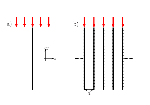
By far the widest used at this time way of the calculation of the electronic response of atomically thin Q2D crystals is the super-cell geometry approach. This is, instead of considering a single layer [schematized in Fig. 1, a)], to artificially periodically replicate it in -direction [Fig. 1, b)], and study the resulting 3D periodic system in place of the original single-layer one. It is, however, known [15, 16, 17] that the 3D dielectric function obtained in the super-cell geometry has nothing to do with that of a single-layer system of interest, unless a special procedure of extracting the 2D response from the 3D super-cell geometry calculation (i.e., the elimination of the spurious inter-layer interaction) is applied. In A we give a detailed derivation of the expression for the density-response function of the single-layer system from - the density-response function of the array system. It reads in the matrix form55 5 In Eq. (38), the full 3D reciprocal space representation for both and is used, which is natural for the former, but may look artificial for the latter. We, however, note that an arbitrary function of and can be expanded in the Fourier series in , and then, if necessary, the real-space representation can be retrieved by the inverse Fourier transform.
| (38) |
where the matrix is given by
| (39) | |||||
| (40) |
The density-response function of the array system can be routinely obtained with the 3D solid-state periodic codes such, e.g., as Elk, abinit, Wien2k, etc.. While is different for different layers’ separations , obtained through Eq. (38) does not depend on , which is crucial for its being a true characteristic of a stand-alone 2D system66 6 Strictly speaking, this is which is independent on . Its Fourier transform in the interval does formally depend on , which is of no physical consequence.. We note that Eqs. (38)- (40) are valid not only in RPA [16], but also in TDDFT with (semi-)local (such as, e.g., ALDA), when different layers interact by the Coulomb potential only.
We conclude this section by noting that the ignoring the fundamental difference between the single-layer response of a Q2D crystal and that of the array of those layers has led to the misinterpretation of the and peaks as single-particle inter-band transitions rather than plasmons [6].
4 Results of calculations and discussion


We have conducted the super-cell geometry calculation for the monolayer pristine graphene followed by the application of Eq. (38) for the extraction of the single-layer response (elimination of the spurious inter-layer interaction) from the 3D calculation. In the DFT super-cell calculation, we used the full-potential linear augmented plane-wave (FP-LAPW) code Elk [19]. The -axis period of the super-cell was taken 20 a.u. The -point grid of , 30 empty bands, and the damping parameter of 0.002 a.u. were used in both the ground-state and the linear-response calculations. The former was conducted within the local-density approximation for the exchange-correlation potential, while the latter was the random-phase approximation (RPA) one (i.e., the exchange-correlation kernel was set to zero). The dielectric matrix of the 3D system was of the size , which was inverted to obtain with the local-field effects included both in the perpendicular and in-plane directions.
Results for the Q2D dielectric and energy-loss functions obtained through Eq. (37) are presented in Fig. 2. Features at the energy-loss function around 5 and 15 eV are usually referred to as and peaks, respectively, [2, 3, 4, 6, 5] (lower panel of Fig, 2). To determine whether they are collective excitations (plasmons) [2, 3, 4, 5] or single-particle (inter-band) transitions [6], we scrutinize the dielectric function.
A clear criterion for an excitation to be classified as plasmon is the requirement of the real-part of the dielectric function to cross zero at the corresponding energy. Otherwise, if the peak at the energy-loss function is due to a peak at the imaginary part of the dielectric function, the excitation is a single-particle transition. In our case, starting from greater wave-vectors (from 0.05 and 0.1 a.u., for and peaks, respectively) the real part of the dielectric function does cross zero, and, thereby, from those -s up the peaks are plasmons unambiguously. Are they also plasmons at smaller -s, or they turn into single-particle transitions, although keeping full similarity to their higher- plasmon counterparts ? To answer this question, we need to establish whether, although does not cross zero at smaller wave-vectors, the features at the energy-loss function are due to approaching zero, or they are due to peaks at (cf., [17]).
As can be seen in Fig. 2, middle panel, Im has prominent non-dispersive (standing in place with the variation of ) feature at 4 eV. A prominent dispersive peak in the energy-loss function (bottom panel) follows the position of not only zero (at greater values of ) but also the minimum (at smaller -s) of Re in the range of 4 - 6 eV, and must, therefore, in both cases be classified as plasmon.
The situation is similar, though less transparent, in the case of the peak. Here, the broad feature at , which spreads from 11 eV upward, is due to the overlap of the single-particle and collective excitations. Up to 14 eV, the excitation is purely due to the single-particle transitions and is non-dispersive. Then, from 14 eV upward, a dispersive feature due to zero or small values of begins. Because of having a low slope and remaining small in absolute value in a wide range, this feature becomes very broad. It, however, is clearly plasmon as well.
Interestingly, in two points, at 8 and 14 eV, becomes nearly unity for all values of , so that all the curves in Fig. 2, upper panel, intersect at these two points. The physical reason for this is still to be understood.
In Fig. 3, the reflection EELS-related energy-loss function , calculated by Eq. (36), is compared with the loss-function of Eq. (37), the latter relevant to the energy dissipation in the in-plane transport . While the features ( 5 eV) are similar for both loss-functions, the features are considerably different, the EELS loss-function having a richer structure in this energy range. This can be understood by noting that, according to Eq. (37), is determined by the head element of the density-response matrix , while, by Eq. (36), the -function also includes contributions from with nonzero and/or . The role of the latter increases with the increase of , transitions into the higher bands becoming allowed, which leads to the differences in the spectra.
In Fig. 4 we compare our theory with reflection EELS experiment of Ref. [18] on monolayer and bilayer graphene. In the energy range of plasmon (two upper graphs in Fig. 4), -function and the energy-loss () function are practically identical and both compare to experiment rather well. On the contrary, in the range of plasmons, the - and -functions acquire differences for both monolayer and, particularly, for bilayer graphene (lower graphs). For bilayer graphene peak at -function is narrower than at the -function, the former being closer to experiment (lower right). Remarkably, for monolayer graphene both - and -functions find themselves in shear disagreement with experiment (lower left).
Obviously, the main source of the disagreement between the theory and experiment can be the presence of the SiC (0001) substrate in the latter and the absence thereof in the former. The substrate may cause additional screening leading to the shift of plasmon peaks and change the dispersion law [20, 21, 22, 23]. Moreover, the interaction of graphene with a substrate can cause the deformation of the graphene sheet, leading to the confinement of the plasmon oscillations between the ripples [24].
Let us briefly discuss the modifications to the theory necessary to include Q2D crystals supported on substrates. For the ab initio theoretical treatment of surfaces, either pure or adsorbates covered, the super-cell method is widely applied as well. In variance with the stand-alone Q2D systems, for surfaces, rather thick slabs of the material alternated with the similar thickness vacuum slabs are used. Equations (38)-(40) are readily applicable in this case too, producing as an output the density-response function of a single slab. This slab having two surfaces is not, however, the semi-infinite system of interest. Neither the array of such slabs, from which we have started, is. Which system, the array of slabs or a single slab, is better to model a Q2D crystal on top of a semi-infinite substrate must be decided in each particular case. An alternative method may be the inclusion of the substrate by means of the effective background dielectric function after having calculated the response of a stand-alone Q2D system. Although it may be useful in some situations, this would necessarily be a phenomenological approach, probably inconsistent with the rigorousness of the calculation for the Q2D crystal alone. Finally, the ultimate theory will be that asymptotically matching Q2D crystal on the surface with the 3D periodic bulk of the substrate, which is a very challenging task.
The neglect of the many-body exchange-correlation effects [25, 26], both static and dynamic, may further contribute to the discrepancy. Both the accurate inclusion of the substrate in the theoretical setup and the inclusion of the many-body effects by means of using nonlocal exchange-correlation kernel of TDDFT remain the major challenges of the present-day theory of Q2D materials.
Figure 5 shows the dispersion of and plasmons with the vector varied in the direction calculated in the EELS setup. The plasmon has a complex structure and is split into distinct sub-excitations.
As noted in Ref. [6], in a 2D system there can be no plasmon at . In the ordinary 2D electron gas [27] and in doped graphene in the case of 2D plasmon due to electrons in the band [28], this is ensured by the plasmon disappearance via its energy tending to zero as when . However, as can be seen from Fig. 2, lower panel, for and plasmons in graphene the same realizes in a different way: The energy positions of these plasmons converge to finite values (4 and 14 eV for and plasmons, respectively) as , while the amplitudes of the corresponding peaks go to zero. In this regard, as in many others, graphene is also special compared to the ordinary 2D electron gas. The zero limit of the plasmons’ amplitude can be understood from simple arguments. Indeed, quite generally, in a 2D crystal, the relation between the dielectric function and the conductivity is
| (41) |
Since in the single-layer graphene, is finite [and known [29] to tend to as ], is unity identically, leading to the zero energy-loss function. Our calculated conductivity of the monolayer pristine graphene at versus the frequency is shown in Fig. 6, where the static limit of is shown by the dotted line.

5 Conclusions
We have identified and dealt with the extra challenges the ab initio theory of electronic excitations in quasi-2D crystals presents in comparison to both the bulk and purely 2D cases. In particular, we have re-examined the problem of the correspondence between the theoretically calculated quantities and the observables in the measurements on quasi-2D crystals and found that the energy-loss function , conventionally used for the interpretation of the EELS data, is not, generally speaking, the right quantity to be compared with this kind of the experiment. Instead, the EELS-related energy-loss functions, specific for both transmission and reflection experimental setups, must be used, which has been shown to be both qualitatively and quantitatively different in the case of quasi-2D systems. In the limit of the zero crystal thickness, our theory reduces to the conventionally used one.
We have addressed the problem of the classification of the and peaks in monolayer graphene. By the use of the accurate procedure of extracting the dielectric function of a 2D crystal from the 3D super-cell geometry calculation, we have shown conclusively that there exist prominent and collective exitations (plasmons) in graphene, although they are accompanied by interband transitions in the close energy ranges. Plasmons and single-particle interband transitions can be distinguished from each other provided the wave-vector-resolved analysis is performed.
We have also demonstrated the importance of the correct interpretation of the super-cell geometry calculation results, the latter taken simplistically, can lead to erroneous qualitative conclusions for materials of reduced dimensionality. We expect that the present theory of the electronic excitations in Q2D crystals, by correctly accounting for the atomic or nano- thickness of the systems studied, will further boost the theoretical and experimental work, improving the methods of comparison between the two.
Appendix A Extraction of the response of a single layer from that of the array-of-layers system
Let us consider a periodic array of identical layers, as schematized in Fig. 1, and let us construct the density-response function of the array system. We assume that the separation between the layers is large enough so that densities, both the ground-state and the dynamically induced, do not overlap between layers. Then for the array system we can write
| (42) |
where
| (43) | |||||
Equation (42) uses the fact that the potential external to the layer is that of Eq. (43), i.e., it is the proper external potential plus the potentials induced by all the layers with . The prime at the sum means that the term is excluded from the summation. Performing the summation explicitly, we have77 7 Equation (44) corrects an error in Eq. (A3) of Ref. [17]. However, all the formulas derived in Ref. [17] under the assumption of , where is the effective width of a layer, remain valid.
| (44) | |||||
Expanding into the Fourier series
| (45) |
where
| (46) |
and introducing the matrices
| (47) | |||||
| (48) |
we arrive at the fully 3D reciprocal-space representation
| (49) |
| (50) |
Using Eqs. (49) and (50), the definition of as the density-response function of the array system
| (51) |
and in view of the arbitrariness of , we can write in the matrix form
| (52) |
It may be useful to consider approximations to the above exact scheme. First, since for , this is practically exact to keep in Eq. (43) the term only. Further, if , where is the effective width of the layer, Eq. (38) can be shown to yield a convenient relation between the corresponding 3D and 2D dielectric functions [17]
| (53) |
where is the dielectric function of the fictitious periodic 3D system comprised of the layers separated by the distance .
In the limit we have from Eq. (53)
| (54) |
In the long-wave limit
| (55) |
which, since the second term is small, can be written as
| (56) |
References
- [1] Politano A and Chiarello G 2014 Nanoscale 6(19) 10927–10940
- [2] Gass M H, Bangert U, Bleloch A L, Wang P, Nair R R and Geim A K 2008 Nature Nanotechnology 3 676–681
- [3] Eberlein T, Bangert U, Nair R R, Jones R, Gass M, Bleloch A L, Novoselov K S, Geim A and Briddon P R 2008 Phys. Rev. B 77(23) 233406
- [4] Liu Y, Willis R F, Emtsev K V and Seyller T 2008 Phys. Rev. B 78(20) 201403
- [5] Liou S C, Shie C S, Chen C H, Breitwieser R, Pai W W, Guo G Y and Chu M W 2015 Phys. Rev. B 91(4) 045418
- [6] Nelson F J, Idrobo J C, Fite J D, Mišković Z L, Pennycook S J, Pantelides S T, Lee J U and Diebold A C 2014 Nano Letters 14 3827–3831
- [7] Liebsch A 1997 Electronic excitations at metal surfaces (New-York: Plenum)
- [8] Nazarov V U 1995 Surf. Sci. 331/333 1157
- [9] Nazarov V U 1999 Phys. Rev. B 59 9866
- [10] Nazarov V and Nishigaki S 2001 Surface Science 482 - 485 640 – 647
- [11] Persson B N J and Zaremba E 1985 Phys. Rev. B 31 1863
- [12] Tsuei K D, Plummer E, Liebsch A, Pehlke E, Kempa K and Bakshi P 1991 Surface Science 247 302 – 326
- [13] Sturm K 1982 Adv. Phys. 31 1
- [14] Wachsmuth P, Hambach R, Kinyanjui M K, Guzzo M, Benner G and Kaiser U 2013 Phys. Rev. B 88(7) 075433
- [15] Rozzi C A, Varsano D, Marini A, Gross E K U and Rubio A 2006 Phys. Rev. B 73(20) 205119
- [16] Despoja V, Novko D, Dekanić K, Šunjić M and Marušić L 2013 Phys. Rev. B 87(7) 075447
- [17] Nazarov V U, Alharbi F, Fisher T S and Kais S 2014 Phys. Rev. B 89(19) 195423
- [18] Lu J, Loh K P, Huang H, Chen W and Wee A T S 2009 Phys. Rev. B 80(11) 113410
- [19] http://elk.sourceforge.net
- [20] Politano A, Marino A R, Formoso V, Farías D, Miranda R and Chiarello G 2011 Phys. Rev. B 84(3) 033401
- [21] Politano A, Marino A, Formoso V, Farías D, Miranda R and Chiarello G 2012 Plasmonics 7 369–376
- [22] Generalov A and Dedkov Y 2012 Carbon 50 183 – 191
- [23] Cupolillo A, Politano A, Ligato N, Perez D C, Chiarello G and Caputi L 2015 Surface Science 634 76 – 80
- [24] Politano A, Campi D, Formoso V and Chiarello G 2013 Phys. Chem. Chem. Phys. 15(27) 11356–11361
- [25] Botti S, Sottile F, Vast N, Olevano V, Reining L, Weissker H C, Rubio A, Onida G, Del Sole R and Godby R W 2004 Phys. Rev. B 69 155112
- [26] Nazarov V U and Vignale G 2011 Phys. Rev. Lett. 107(21) 216402
- [27] Stern F 1967 Phys. Rev. Lett. 18 546–548
- [28] Das Sarma S and Hwang E H 2009 Phys. Rev. Lett. 102(20) 206412
- [29] Wunsch B, Stauber T, Sols F and Guinea F 2006 New Journal of Physics 8 318