A User-Friendly Dark Energy Model Generator
Abstract
We provide software with a graphical user interface to calculate the phenomenology of a wide class of dark energy models featuring multiple scalar fields and potentials that are arbitrary functions of exponentials. The user chooses a subclass of models and, if desired, initial conditions, or else a range of initial parameters for Monte Carlo. The code calculates the energy density of components in the universe, the equation of state of dark energy, and the linear growth of density perturbations, all as a function of redshift and scale factor. The output also includes an approximate conversion into the average equation of state, as well as the common parametrization. The code is available here: http://github.com/kahinton/Dark-Energy-UI-and-MC
I Introduction
The puzzle of dark energy is one of the most important outstanding questions in all of physics. Studying the observational signatures of dark energy – and using those signatures to understand the nature of dark energy – has been a highly active area of research since the first signs of dark energy were discovered over 15 years ago. (For a review, see e.g. Frieman et al. [1].) Dark energy models have a rich phenomenology, leaving varied fingerprints on the growth of cosmic structure and on geometrical quantities in the universe.
We have written a piece of software that makes it easier to compute quantitative predictions for dark energy models broader than a simple cosmological constant. These models possess a richer phenomenology that can be tested with ongoing and future experiments. They also complement the choice of dark energy models – and computer code – made by others [2]. Our software is capable of handling a wide class of models with multiple scalar fields, and specifically makes two subclasses particularly easy to calculate with a simple user input. In these models, the user can calculate the expansion history and the growth of structure in the linear regime, therefore enabling the user to obtain various implications for observable quantities in cosmology. The code also returns an approximate conversion of the equation of state of dark energy into two commonly used parameters , as well as several other commonly used parameters.


II Dark Energy Models
We choose two classes of “assisted dark energy” models, based specifically on the analysis by Ohashi and Tsujikawa [3], and originally developed by Refs. [4, 5]. The starting assumption is the existence of scalar fields, and a Lagrangian density that takes the following form
| (1) |
where is the kinetic term for -th field, and is an arbitrary function of its argument , where is a dimensionless parameter. The existence of scaling solutions dictates that this be the most general form of the Lagrangian density for exponential potentials [4, 5]. A noteworthy special case of our class of models is quintessence with a single field (), and a simple exponential potential , for which . As we explain below, this class of models also includes ghost condensate models [6] featuring a background scalar field which, despite having a kinetic term of the “wrong” sign, are stable and feasible due to suitable higher-order kinetic terms.
Our code allows a user to test models with an arbitrary function , for an arbitrary number of fields . As an example we also provide two special cases which have been run through the Monte Carlo generator, and whose results can be accessed with very simple inputs in the graphical user interface (GUI):
| (2) | |||||
| (3) |
In each case, the temporal evolution of all quantities is most easily tracked in terms of scaled variables
| (4) |
where is the radiation energy density. The evolution equations, expressed in terms of the time variable , are [3]
| (5) | |||||
| (6) |
We numerically evolve these equations. Then all physical quantities of interest can be found, for example the energy densities of matter and dark energy
| (7) |
and the dark energy equation of state
| (8) |
where the time-dependent parameter can be calculated via . Note that for quintessence, the functional form of in Eq. (2) implies that the potential is the sum of exponential potentials for each field, .
III Using the Provided Software
Our code can be found at the following GitHub repository: http://github.com/kahinton/Dark-Energy-UI-and-MC. The code gives the user several tools for testing and analyzing various models of dark energy. The first step in being able to use these tools is to run a model through our Monte Carlo generator. The user must supply several inputs to the MC generator: a specific function , as described above; a name to differentiate the model from others; and the number of different initial conditions to test the model over. The provided name will be used to label this model in the user interface. The user must also specify the values for several parameters governing each model. Specifically these parameters are the number of fields that will be acting as dark energy, , as well as the range for the initial conditions of , , , and . In our code we adopt a simplification suggested in [3], which assumes that a single field will act to assist inflation in the early universe before becoming small, while the remaining fields will be small in the early universe before becoming the dominant form of energy at late times. The “assisted inflation” field will have one set of unique initial conditions, while the remaining fields will all share the same initial conditions. This later simplification drives the value of as close to as possible at late times, and also allows models to be tested at the same speed independent of the number of fields being used.

By using these simplifications the user only needs to specify the range of initial conditions for the first two fields. The code then assumes, for example, that all values of to are equal. To ensure that a scalar field dominated solution is produced, the values for are chosen automatically, according to the inequalities (see Eqs. (29) and (32) in [3])
| (9) |
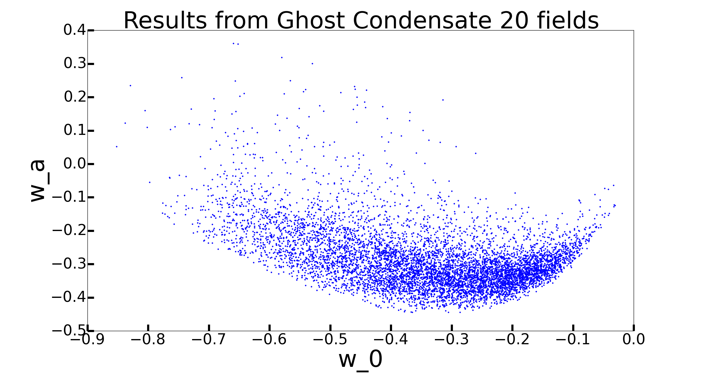
Here is the Lagrangian density, and . When the code is run, for each specific test, the initial conditions for each parameter are chosen from a random flat distribution over the selected range. When all of the tests have finished running the model will be added to the user interface automatically. As an example of what is output to the user interface, we have included the results of tests of quintessence and ghost condensate models having 5, 10, 15, and 20 fields.
The user interface also contains two optional tools. The first of these allows the user to run a single instance of any model having been run through the Monte Carlo generator. Each of the required parameters are assigned a set of fiducial values that depend on which model is chosen; however, the range over which the model has been tested is also supplied, allowing the user to experiment with values other than those provided. Once the user selects values for these parameters, they can choose to plot various quantities as a function of either scale factor or redshift . These quantities include:
- •
Energy densities in units of critical (radiation , matter , dark energy );
- •
Equation of state of dark energy ;
- •
Linear growth of density fluctuations (we plot the quantity ).
In order to provide the growth of linear perturbations, concurrently with the other equations we also evolve
| (10) |
where is the linear growth rate of matter perturbations, and where the primes indicate a derivative with respect to . The quantity for the selected model will immediately be displayed on screen for the user to examine.
The second option available to the user is to examine the results from the Monte Carlo generator. Specifically, this tool allows the user to generate two-dimensional scatterplots on the fly for further analysis – for example, to see what range of phenomenological outcomes is produced by a given model or class or models. Each point in a given scatterplot corresponds to an output of a single model. The output can be any of the following parameters or functions:
- •
Initial conditions from each model including , , , , , , , , , and ;
- •
Energy densities in matter and dark energy today and , as well as the equation of state today .
- •
Effective “average” equation of state , calculated from the first principal component, as described in the Appendix.
- •
Effective values for the parameters and based on parametrization [8] , derived from the first two principal components as described in the Appendix.
An example of the Monte Carlo output showing the plane is shown in the right panel of Fig. 3.
Acknowledgments
We thank Eric Linder for useful comments. Our work has been supported by NSF under contract AST-0807564 and DOE under contract DE-FG02-95ER40899.
Appendix A Appendix: Principal components, , and ()
Here we explain in more detail how to calculate the aforementioned quantities , , and from the principal components of the equation of state, following [9, 10]. First, we formally expand the equation of state in terms of principal components
| (11) |
where is the coefficient of the -th principal component . The idea is to convert the first principal component into the averaged value of the equation of state , and first two principal components into . This approach is justified because the first few principal components carry essentially all the necessary information about the effects of dark energy dynamics on the expansion of the universe on observable scales.
The principal components can be determined for any given dataset; here we use the Figure of Merit Science Working Group’s (FoMSWG) publicly available code [7], and a combination of Planck+BAO+SN+WL available in their code. Note that, while the component shapes — especially the all-important peak value of that shows the temporal epoch of maximum sensitivity to the equation of state — depend on the cosmological probe as well as specifications of a given experiment, once we combine the probes the pull of different probes is expected to average out, leading to a fixed set of shapes.
While the normalization of the is arbitrary in principle, the FoMSWG principal components that we use are normalized as . The coefficients can be obtained as
| (12) |
where is the actual equation of state of the theoretical dark energy model we are studying.
The final step is converting the first principal component into , and the first two into and ; we do this via [10]
| (13) |
and
| (14) |
where are defined in Eq. (12), and
| (15) |
Equations (13) and (14) are now our definitions of the parameters and , respectively, given a dark energy history which determines the . Previous work [10] confirms that the two-parameter equation of state closely follows the true over the redshift range most effectively probed by the data.
Note too that the constraint , which follows from , is not strictly obeyed by obtained in this way since and are now essentially a fit to the dark energy equation of state history. In other words, the derived parameter can be slightly smaller than ; this is again because we are fitting these three -parameters and forcing them to the model’s actual equation of state evolution. These parameters are nevertheless provided since 1) they provide a very useful test bed to gauge the effectiveness of the range of dark energy model behavior, and 2) they are fairly representative of these models, since actual dark energy models often do exhibit the scaling.
References
- [1] J. Frieman, M. Turner, and D. Huterer, Ann.Rev.Astron.Astrophys. 46, 385 (2008), arXiv:0803.0982 [astro-ph] .
- [2] D. J. Marsh, P. Bull, P. G. Ferreira, and A. Pontzen, Phys.Rev. D90, 105023 (2014), arXiv:1406.2301 [astro-ph.CO] .
- [3] J. Ohashi and S. Tsujikawa, Phys.Rev. D80, 103513 (2009), arXiv:0909.3924 [gr-qc] .
- [4] F. Piazza and S. Tsujikawa, JCAP 0407, 004 (2004), arXiv:hep-th/0405054 [hep-th] .
- [5] S. Tsujikawa and M. Sami, Phys.Lett. B603, 113 (2004), arXiv:hep-th/0409212 [hep-th] .
- [6] N. Arkani-Hamed, H.-C. Cheng, M. A. Luty, and S. Mukohyama, JHEP 0405, 074 (2004), arXiv:hep-th/0312099 [hep-th] .
- [7] A. Albrecht, L. Amendola, G. Bernstein, D. Clowe, D. Eisenstein, et al., (2009), arXiv:0901.0721 [astro-ph.IM] .
- [8] E. V. Linder, Phys.Rev.Lett. 90, 091301 (2003), arXiv:astro-ph/0208512 [astro-ph] .
- [9] D. Huterer and G. Starkman, Phys.Rev.Lett. 90, 031301 (2003), arXiv:astro-ph/0207517 [astro-ph] .
- [10] D. Huterer and H. V. Peiris, Phys.Rev. D75, 083503 (2007), arXiv:astro-ph/0610427 [astro-ph] .