Early-time cosmological solutions in Einstein-scalar-Gauss-Bonnet theory
Abstract
In this work, we consider a generalised gravitational theory that contains the Einstein term, a scalar field and the quadratic Gauss-Bonnet term. We focus on the early-universe dynamics, and demonstrate that a simple choice of the coupling function between the scalar field and the Gauss-Bonnet term and a simplifying assumption regarding the role of the Ricci scalar can lead to new, analytical, elegant solutions with interesting characteristics. We first argue, and demonstrate in the context of two different models, that the presence of the Ricci scalar in the theory at early times, when the curvature is strong, does not affect the actual cosmological solutions. By considering therefore a pure scalar-GB theory with a quadratic coupling function we derive a plethora of interesting, analytic solutions: for a negative coupling parameter, we obtain inflationary, de Sitter-type solutions or expanding solutions with a de Sitter phase in their past and a natural exit mechanism at later times; for a positive coupling function, we find instead singularity-free solutions with no Big-Bang singularity. We show that the aforementioned solutions arise only for this particular choice of coupling function, a result that may hint to some fundamental role that this coupling function may hold in the context of an ultimate theory.
I Introduction
In the quest for the final theory, that would unify the gravitational interactions with their particle physics analogs and describe them correctly at arbitrarily large energy scales, the generalised gravitational theories have played a primary role. In their majority, these theories are purely geometrical in nature and involve extra dimensions: well-known examples are superstring theory [1], the Lovelock theory [2] or the novel theories with extra dimensions [3, 4]. For a 4-dimensional observer, however, the dynamics and content of this higher-dimensional, fundamental theory is translated into the appearance of new terms, describing gravity or a number of additional fields, in the context of the 4-dimensional effective theory. Inspired by the aforementioned theories, many variants of modified gravitational theories have been constructed over the years, and their implications for gravity and cosmology were extensively studied.
The most usual way to modify the gravitational interactions in a 4-dimensional context is via the addition of gravitational terms that involve higher powers of curvature. In the context of the heterotic superstring effective theory [5, 6, 7], for instance, the Einstein term is supplemented by quadratic curvature terms, such as the Gauss-Bonnet term or the term with the latter, however, being trivially zero for a Friedmann-Lemaître-Robertson-Walker background. The Gauss-Bonnet term is also the first-order correction to the Einstein term in the Lovelock theory, that is considered as a natural generalisation of Einstein’s theory of gravity in a higher number of dimensions [8]. In 4 dimensions, however, the Gauss-Bonnet (GB) term is a topological invariant and adds nothing to the field equations of the theory unless it is coupled to an additional field. Inspired by superstring theory, the usual way is to couple the GB term to a scalar field. By doing that, the GB term remains in the theory and has been shown to lead to a variety of new solutions: singularity-free cosmological solutions [9, 10], novel hairy black holes [11, 12] or even traversable wormholes [13] – solutions that were absent in the traditional General Relativity that contains only the Ricci scalar term (for a review on this type of generalised gravitational theories and further references, see [14]). Also, since the field equations remain second order for the Lovelock theory in general and GB in particular, they are widely known to be ghost-free theories contrary to some brane models like DGP (see e.g. [15] for a summary) or higher-derivative theories, which often suffer from the Ostrogradski ghost [16] (however, see [17] for a counterexample). These theories have also been intensively studied in various realistic contexts: by considering solar system constraints [18], as a dark energy model with CMB and galaxy distribution constraints [19] or as an inflationary model [20, 21].
In this work, we will focus on the dynamics of early universe and look for the corresponding cosmological solutions. During the early universe, it is natural to expect that a string-inspired theory would describe better its dynamics – that is why here we consider a 4-dimensional theory containing the Einstein term and a scalar field (one of the many of string theory) coupled non-minimally to gravity through a general coupling function to the quadratic Gauss-Bonnet term. However, we will go one step beyond that: we will demonstrate, in the context of two different models, that the presence of the Ricci scalar adds nothing to the dynamics of the universe at early times where the curvature is strong; in fact, it is the coupled system of scalar field and GB term that dominates and governs the evolution of the universe. Motivated by this, we will then look for and derive, exclusively via analytical means, cosmological solutions with interesting characteristics in the context of the pure scalar-GB theory. For the particular case of a quadratic coupling function between the scalar field and the GB term, we will present two classes of solutions that are distinguished by the sign of the coupling function constant: for a negative coupling constant, the system of equations supports cosmological solutions that are either purely de Sitter-like or have a de Sitter inflationary phase in their past and a natural exit mechanism at later times; for a positive coupling constant, a class of singularity-free solutions emerges instead.
Although these solutions are derived for a particular form of the coupling function, it has been shown in the past that a polynomial, even coupling function, such as the quadratic one chosen here, shares many common characteristics with the actual coupling function between the moduli fields and the GB term in the heterotic superstring effective theory [10]. Therefore, our present analysis, that proposes a new approach in deriving early-time cosmological solutions, will be of relevance to the superstring effective theory itself, but also to any other generalised, string-inspired theory that contains the GB term coupled to a scalar field. All these theories are bound to have in the phase-space of their solutions, the aforementioned classes of solutions as early-time asymptotics. In addition, the analytical derivation of the solutions, in contrast to the usual numerical means employed systematically when the Ricci term is kept in the theory, allows for a more comprehensive study of the properties of the found solutions. The presence of the Ricci scalar inevitably becomes important, as the universe expands, and a transition between the scalar-GB-dominated phase and a subsequent one that prepares the universe for a traditional Ricci-scalar-driven cosmology will eventually take place. Such a transitory phase is studied at the final part of this work.
Our approach is very similar to the two important conjectures about asymptotic dynamics at early times proposed by Belinsky, Khalatnikov and Lifshitz (BKL). The two conjectures state that matter content [22, 23] and spatial derivatives [24] are not dynamically significant near the initial singularity. With the same spirit, we will conjecture and prove in a class of models that lower-curvature terms in the Riemann tensor are negligible near the singularity compared to higher-curvature terms.
The outline of our manuscript is as follows: in Section 2, we present the theoretical framework of our analysis and the derived set of field equations. In Section 3, through the use of a toy model, we demonstrate how the presence of the Ricci term in the theory merely complicates the analysis without changing anything in the actual dynamics of the solution. We reinforce this argument in Section 4, where the complete theory of the Ricci scalar, a scalar field and the Gauss-Bonnet term is studied for the case of a linear coupling function. In Section 5, we consider the pure scalar-GB theory with a quadratic coupling function, and derive a variety of early-time cosmological solutions with attractive characteristics. In Section 6, we briefly consider the case of a general polynomial coupling function, and in Section 7, we study an indicative transitory phase for the universe as it passes from a scalar-GB-dominated phase to one where the Ricci scalar starts being important. We present our conclusions in Section 8.
II The Theoretical Framework
In this work, we consider a string-inspired gravitational theory that contains, apart from the Ricci scalar, a scalar field coupled non-minimally to gravity via a general coupling function to the quadratic Gauss-Bonnet term. Such a theory is described by the following action functional
| (1) |
where the Gauss-Bonnet term is defined as
| (2) |
Since the focus of this work will be the dynamics of the universe at very early times where high-energy and strong-curvature effects are expected to be the dominant ones, throughout this work, we will assume that any additional distribution of matter or energy, apart from the scalar field, plays only a secondary role and thus will be ignored.
The variation of the action (1) with respect to the scalar field and the metric tensor leads to the scalar and gravitational field equations, respectively; these have the form
| (3) |
and
| (4) |
where , and is defined as
| (5) |
We note that if, the Gauss-Bonnet term is altogether ignored in the theory, the scalar field looses its potential; on the other hand, if the scalar coupling function is a constant, then and the contribution of the Gauss-Bonnet term to the gravitational field equations (4) vanishes. We may therefore conclude that and seem to form an independent pair of quantities that mutually support each other. Recall that it is the metric that acts as potential in General relativity and it is coupled to the velocity, , in the Lagrangian, , for particle motion. It should be noted that the coupling of the scalar field with the Gauss-Bonnet term is in the same general relativistic form and spirit. It is therefore a very desirable feature of the theory.
We will also assume that the line-element has the Friedmann-Lemaître-Robertson-Walker form
| (6) |
that describes a homogeneous and isotropic universe with a scale factor and spatial curvature . For the above metric ansatz, the Gauss-Bonnet term takes the explicit form
| (7) |
where is the Hubble parameter and the dot denotes derivative with respect to time. Using the above geometrical quantities, the scalar (3) and gravitational field equations (4) reduce to the following system of three, ordinary but coupled, differential equations
| (8) | ||||
| (9) | ||||
| (10) |
In the following sections, we will look for cosmological solutions supported by the above set of equations both in the presence and in the absence of the Ricci scalar. We will start with a simple toy model, that will demonstrate the role of the Ricci scalar in the context of the complete theory; the same task will then be performed in the framework of a less restricted model. Using the derived insight of when the Ricci scalar may be ignored from the theory, we will then search for solutions where the Ricci scalar is negligible compared to or of the same order as the Gauss-Bonnet term.
III A Toy Model
In this section, we will look for solutions of the set of Eqs. (8)-(10) on which we impose the constraint of the vanishing of the Gauss-Bonnet term, . The is then a solution of the scalar field equation which is trivially satisfied. But, the Einstein’s equations, since now , demand that the following two constraints
| (11) |
should be simultaneously satisfied. As it was shown in [10], for , the above equations lead to a static universe with an arbitrary or infinite radius, respectively, while for we obtain a linearly expanding universe with and a singularity at a finite time.
We will thus search for solutions with . Since , the scalar equation is easily integrated once to give
| (12) |
where an arbitrary integration constant. The solution for the scale factor is most easily given by the constraint itself, or equivalently
| (13) |
where the two multiplying factors could be independently zero or not. In fact, it is only for the second choice, , that a non-trivial solution for the scalar field is allowed. Then, we easily find that again, but now this solution holds for all values of . Taking the sum of Eqs. (9)-(10), we find the constraint
| (14) |
with solution
| (15) |
where are again integration constants. The scalar field itself can easily be found from Eq. (12) to have the form
| (16) |
From a field-theory point-of-view, it would be much preferable to express the coupling function in terms of the field instead of the time coordinate. Comparing the above two equations, and upon a convenient choice of the integration parameter , i.e. , we see that we can write
| (17) |
where are constants given in terms of .
Let us now ignore the presence of the Ricci scalar in the theory. Since the scalar-field equation (8) and the constraint (13) remain unaltered, both the solution for the scalar field (16) and the linearly-expanding form of the scale factor are still valid. However, the Einstein field equations now take the simplified from
| (18) |
| (19) |
which, when combined with each other, lead to the constraint
| (20) |
for the coupling function. The above can be easily integrated and expressed in terms of the scalar field to obtain
| (21) |
Therefore, assuming that the Ricci scalar can be ignored, we obtain the same solutions for the scalar field and scale factor as in the presence of it, with the only change appearing in the expression of the coupling function that now takes a simpler form. Looking more carefully, the two expressions (17) and (20) are equivalent in the limit where the scalar field takes very large values; from Eq. (16), this happens as we approach the initial singularity, . Therefore, as expected, in the presence of the quadratic Gauss-Bonnet term in the theory the Ricci scalar adds nothing to the dynamics of the universe at the very early-time limit.
IV The Complete Theory with a Linear Coupling
In this section, we will attempt to reinforce the conclusion drawn in the previous section regarding the role of the Ricci scalar in the early-universe cosmology but in the context of a more realistic set-up. We will therefore look for physically-interesting solutions following from the complete set of Eqs. (8)-(10) under the assumptions that the Gauss-Bonnet term is not zero and that the function is a non-trivial function of the field . Then, using the relations
| (22) |
and adding Eqs. (9) and (10), we end up with the constraint
| (23) |
We may now use Eqs. (8) and (9) to replace the combination and in the second and third term, respectively, of the above equation. Then, we arrive at
| (24) |
In this work, we will consider a polynomial form for the scalar coupling function, i.e. , where a constant and an integer. The case with results into a constant coupling function and is equivalent to ignoring the Gauss-Bonnet term from the theory. The particular case of will be studied in this section while the case with will be considered in Section 5.
Let us therefore focus on the scalar equation (8) and use that ; then, it can be brought to the form
| (25) |
which can be straightforwardly integrated to yield the relation
| (26) |
with an integration constant. The second term in the above expression, proportional to the coupling constant , is clearly the one associated to the Gauss-Bonnet term, while the first one appeared also in Eq. (12) in the absence of a potential. As we are now interested in studying the properties of solutions arising in the presence of the quadratic GB term, we will set for simplicity , and make a comment on the role of a non-vanishing value of later in this section.
For the case of linear coupling, Eq. (24) is also simplified since . Moreover, we may use Eq. (9) to replace the combination in terms of . Then, Eq. (24) takes the simpler, more explicit form
| (27) |
Now, keeping only the second term in Eq. (26) and using this relation to substitute in the equation above, the latter constraint is finally rewritten as
| (28) |
The above equation does not involve anymore, and it can be integrated once to give
| (29) |
with an integration constant again. Unfortunately, for , the above cannot be easily solved for to yield, via another integration, the form of the scale factor. However, for the case of a flat universe (), we easily write that
| (30) |
with solution
| (31) |
In the above, stands for the hypergeometric function whose convergence demands that – from Eq. (29) and for , it follows that must be indeed a positive constant for a real solution for the scale factor to exist. As a result, the scale factor is bounded from above with the constant determining its upper value. On the other hand, in the limit , the hypergeometric function goes to unity, and the relation between the scale factor and the time coordinate becomes linear; this of course signals the existence of a singularity at a finite value of the time-coordinate. Figure 1 depicts the profile of the scale factor as it starts from the initial singularity, follows an increasing phase and eventually reaches its maximum value determined by . The value of the coupling parameter affects the slope of the uprising curve at early times.

Let us make, at this point, a comment on the role of a non-vanishing value of the parameter . If we keep both terms in Eq. (26) and follow a similar analysis as above, then, for again, we obtain, instead of Eq. (30), the following equation
| (32) |
The above is again difficult to solve for and integrate further, however, we may study particular limits. For a non-vanishing value of , ignoring the first two terms, as we did in the analysis above, would still be justified in a regime where takes very large values. Drawing experience from the known cosmological solutions, we know that the rate of expansion of the universe is the largest close to the initial singularity; as we are indeed interested in the early-universe dynamics, the role of is therefore negligible and our assumption was justified.11 1 For completeness, let us note that in a regime where would be very small and thus the first term on the right-hand-side of Eq. (32) would dominate instead, the corresponding solution for the scale factor is given by the form . For intermediate values of , where the second term in Eq. (32) would dominate, the scale factor behaves as .
Looking for further support to our argument that the presence of the Ricci scalar adds very little to the dynamics of the early-time cosmological solutions, we will now adopt a different approach: we will focus on the early-time limit, and ignore from the beginning the Ricci scalar from the field equations. In the absence of , the gravitational equation (18) can be straightforwardly solved for to yield
| (33) |
even for a general coupling function and without any need for integration. If we then follow a similar analysis as at the beginning of this section, i.e. take the sum of Eqs. (18) and (19), and use the scalar equation (8) and Eq. (33) in there, we obtain the new constraint
| (34) |
The quantity is not allowed to be zero since then the Gauss-Bonnet term would be eliminated from the theory. The same holds for the combination since this term is part of both the Gauss-Bonnet expression and , Eqs. (7) and (33) respectively. Therefore, it is the expression inside the square brackets that should vanish instead; for a general polynomial form of the coupling fucntion, , this may be re-written as
| (35) |
Therefore, for the linear case with , the second term in the above equation vanishes which leaves us with a much simpler constraint: its general solution is a linear function of time, i.e. . This is in accordance to the behaviour obtained in the first part of this section when the early-time limit of the complete solution (31) was considered. The dashed lines in Fig. 1 represent the linear-in-time solution for the scale factor, derived above in the absence of the Ricci scalar in the theory - the agreement with the early-time behaviour of the complete solution is more than evident. Therefore, we conclude again that, by ignoring the presence of the Ricci scalar, we significantly simplify the analysis and still obtain exactly the same early-time cosmological solution.
As we anticipate from the above, the solution for the scalar field may be derived, in the same early-time limit, from either Eq. (26) with or from its simpler analog (33): in both cases, we easily obtain that at early times
| (36) |
where , , and are arbitrary integration constants. The above describes a decaying scalar field as the universe expands with a singular behaviour at the initial singularity.
V The Scalar-GB Theory with Quadratic Coupling
In this section, we address the case of the quadratic coupling function of the scalar field to the Gauss-Bonnet term, . The constraint (24), derived in the context of the complete Einstein-scalar-GB theory, is valid for an arbitrary , therefore it could be applied for this case, too. However, the scalar equation (8) now cannot be easily integrated, and as a result the set of field equations cannot be decoupled. Despite our persistent efforts, no way forward could be found via analytical calculations.
Nevertheless, if one is interested strictly in the early-universe dynamics, the results of Sections 3 and 4 point towards ignoring the Ricci term from the very beginning in order to simplify the analysis and increase the chances of deriving viable cosmological solutions via analytical means. Equation (35), valid in the context of the pure scalar-Gauss-Bonnet theory, has been derived for a general polynomial coupling function and it can be applied directly for the quadratic case with . In that case, the -dependence disappears and the constraint becomes a differential equation only for the scale factor . It can be conveniently separated as follows
| (37) |
leading eventually, after integrating both sides with respect to time, to the relation
| (38) |
In the above, is an arbitrary integration constant. For , the above relation is of a transcendental form and thus impossible to solve for . We are thus forced to consider again the case of a flat universe, in which case we obtain the simple differential equation
| (39) |
In fact, a variety of cosmological solutions with interesting characteristics may be derived from the above simple equation depending on the values of the integration constant and the Gauss-Bonnet coupling parameter . Below, we present a comprehensive analysis of all the ensuing solutions.
V.1 The case with

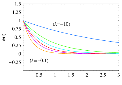
If , then from Eq. (39) it is clear that solutions exist only for . In this case, a simple integration yields the solution:
| (40) |
The theory admits both increasing and decreasing solutions for the scale factor with respect to time - choosing the positive sign, we obtain an exponentially expanding universe with no singularities at finite values of the time coordinate. Note that no self-coupling potential needed to be introduced for the scalar field or tailored in any ad hoc way in order to obtain inflation. Instead, it is the coupling of the scalar field to the quadratic Gauss-Bonnet term that provides a potential in the most natural way and supports inflationary solutions in the early universe. Such couplings arise naturally both in the context of string-inspired or gravitationally modified theories, and we anticipate that they should all contain similar inflationary solutions - by insisting, however, in keeping the Ricci scalar in the analysis, these solutions were missed.
The form of the scalar field, in turn, may be easily found via Eq. (33), that now takes the form
| (41) |
Employing the solution for the scale factor (40) found above (with the positive sign), the scalar field is found to have the form
| (42) |
The scalar field is also everywhere well-defined and is decaying exponentially from an arbitrary initial value to zero. The profiles of both the scale factor and the scalar field are shown in Figs. 2(a,b), respectively, for the values and 10; we observe that the smaller the value of the coupling constant , the faster both quantities evolve with time.
The effective potential of the scalar field receives contributions from both the coupling function and the Gauss-Bonnet term, and has the form . Further aspects of this de Sitter solution were studied in a previous short work [25]. In there, we showed that the necessary number of e-foldings follow easily without the need for assuming trans-planckian initial values for the scalar field. As a result, the effective potential, although of a similar form to that of chaotic inflation [27], remains always bounded. Its dependence on the coupling constant allows also for its value, at the time of inflation, to be large enough so that it dominates indeed over the other constituents of the universe. Finally, its quadratic form places it in the group of inflationary models that are still compatible with the current observational constraints [31].
V.2 The case with and
We now assume that the coupling parameter is again negative as before, but we allow the integration constant to take positive values. This class of solutions first appeared in [25] but we include it also in the analysis here for completeness and for providing additional mathematical details left out in the previous work. In this case, Eq. (39) can be rewritten as:
| (43) |
where . By setting and using standard techniques of integration, the above equation eventually leads to the result
| (44) |
For , i.e. in the absence of the Gauss-Bonnet term, we smoothly recover the linearly expanding solution found in Section 3. For , Eq. (44) is of a transcendental form and thus cannot be solved for as a function of . Its behaviour in terms of time is nevertheless depicted in Fig. 3: choosing the (+)-sign, we find that the scale factor is expanding with time, first with a much faster pace and later with a significantly slower one. As increases, the point where the scale factor vanishes, i.e. the initial singularity, moves gradually towards larger negative values of the time coordinate; on the other hand, for larger values of time, the variation of affects much less the rate of expansion. We may derive analytic asymptotic solutions describing the behaviour of the scale factor at early times and later times, by taking appropriate limits of the complete solution (44). To this end, we first consider the limit , in which case we recover the pure de Sitter solution (40) found in the previous subsection; we thus conclude that the families of solutions with and with and are smoothly connected in the phase-space of the theory. On the other hand, expanding for large values of , i.e. for , we obtain a linear function of time for the scale factor. Therefore, in this class of solutions, the universe interpolates between a pure de Sitter solution at very early times, triggered by the Gauss-Bonnet term, and a linearly-expanding Milne-type phase at later times when the effect of the Gauss-Bonnet term starts to wear off. In this way, these solutions may readily accommodate an early inflationary phase with a natural exit mechanism at later times.

The solution for the scalar field should in principle follow from Eq. (33), however the absence of an explicit solution for the scale factor in terms of time complicates the necessary integration. However, we may find an implicit expression for the scalar field in the following way: if we use Eq. (33), then Eq. (35) may be re-written, for a general polynomial coupling function, as
| (45) |
which, upon integration of both sides with respect to time, gives the constraint
| (46) |
Specialising for the case and , and using Eq. (39) to replace , we finally obtain
| (47) |
Using the asymptotic behaviour of the scale factor at early times, i.e. the pure de Sitter solution (40), we may easily conclude that the scalar field also assumes its exponentially decaying form of Eq. (42). On the other hand, for , the scalar field reduces to a constant.
V.3 The case with and
We will next assume that again, but that now. From Eq. (39), we may see that any solutions that would follow in this case will not allow the scale factor to grow indefinitely but only up to a maximum value, otherwise the rate of expansion would become imaginary. Equation (39), for this choice of parameters, can be alternatively written as:
| (48) |
where . We now set , and by integrating once we find the result
| (49) |
The profile of the scale factor in terms of time, as this follows from the above relation for the positive sign, is depicted in Fig. 4. The early-time behaviour of the above solution is very similar to the one found in the previous subsection: a singularity, where , is again present but this is reached at increasingly large negative values of the time coordinate as increases; the expansion of the relation (49) in the limit leads once again to the pure de Sitter solution (40) and to an inflationary phase for the universe. However, the quantity is now the maximum allowed value of , and the universe stops increasing after this point. We thus conclude that, in the phase space of the solutions of the theory, the pure de Sitter solutions for and branch off to two families of cosmological solutions with totally different behaviour at larger times: one that allows for indefinite expansion of the universe for and one where the scale factor reaches a ceiling for .

The solution for the scalar field follows again from Eq. (46) and in this case is given by
| (50) |
Again, in the early-time limit where , the scalar field adopts the exponentially decaying form of Eq. (42). On the other hand, for , the scalar field goes to zero. As in the previous case, the scalar field remains finite and diverges only at the initial singularity where the scale factor vanishes.
V.4 The case with and
We now reverse the sign of the coupling parameter and allow it to take only positive values. In that case, the choices are not allowed, and mathematically consistent solutions may be derived only for . In this case, Eq. (39) can be rewritten as:
| (51) |
where . We now set , and upon integrating, we find the relation
| (52) |
For , i.e. , we may easily see that we go back to a linearly expanding solution with an initial singularity at a finite value of the time coordinate. However, for , i.e. in the presence of the Gauss-Bonnet term, the situation is radically different: the square-root on the left-hand-side demands that , therefore becomes the smallest allowed value of the scale factor in this model, and no singularities are allowed to arise. The same conclusion follows from the inverse cosine function whose argument should also satisfy the inequality , or in our case since both and are positive-definite. If we expand the solution (52) for values of close to its minimum value , we find the asymptotic solution
| (53) |
which shows its regular behaviour for any finite values of the time-coordinate. In Fig. 5, we plot the behaviour of the scale factor as a function of time: the different curves correspond to different values of from left to right. We observe that as increases the curve is moving towards larger values of and thus away from the singularities. For large values of , the dependence becomes linear again in terms of time – note that this behaviour is common for the two solutions arising for .

The implicit solution for the scalar field in this case is given by
| (54) |
Since the minimum value of the scale factor is , the above expression for the scalar field remains always finite. It starts from a zero value at very early time, it follows an increasing profile reaching eventually a constant value.
Let us comment at this point on the implications of the existence of this particular class of solutions. Singularity-free solutions arising in the context of string-inspired theories, or modified gravitational theories in general, are always important as they provide an alternative to the cosmological solutions of the classical theory of General Relativity that always possess an initial (or final) singularity. Solutions free from the initial singularity have been derived, for instance, in the context of the heterotic superstring effective theory [9]. In there, the coupling function between the scalar field and the Gauss-Bonnet term is given by the highly non-trivial expression , where is the Dedekind function. However, in [10] analytical arguments were presented that showed that singularity-free solutions may arise in the context of a similar theory where the coupling function has a much simpler form, namely , where was strictly an even, positive number – specific solutions were found numerically in the context of the same work. The reason was that these two different forms share in fact three important characteristics: they are invariant under the change , they have a global minimum and asymptotically they tend to infinity.
In the present work, we have indeed managed to derive an analytical singularity-free solution for the even coupling function , in total agreement with the aforementioned argument. Note, however, that the analysis of [10] took into account the presence of the Ricci scalar in the theory thus forcing the authors to perform numerical integration in order to find the sought solutions. Here, by ignoring the Ricci scalar, we have managed to demonstrate in a very simple way the emergence of singularity-free solutions and to find their exact analytical form. We believe that this result solidifies even more our argument that the Ricci scalar may indeed be ignored in the early-time limit with no effect in the dynamics of the universe and that, in fact, one should do so, in order to derive elegant, analytical solutions.
VI The Case of a General Polynomial Coupling Function
In this section, we will briefly address the case of a general polynomial coupling function, . Both Eqs. (35) and (46) have been derived for this case, and thus can be straightforwardly used for our purpose. Solving Eq. (46) for the scalar field and substituting in Eq. (35), we obtain the constraint
| (55) |
with
| (56) |
Specializing to the case of a flat universe with , we obtain
| (57) |
We can easily check that the above equation admits de Sitter-type solutions only for particular values of the integer . Setting , the aforementioned equation becomes
| (58) |
According to the above, consistent de Sitter-type solutions arise only for , and for or equivalently , in accordance to the results of Section 5.
If we integrate Eq. (57) with respect to time once, we find the relation
| (59) |
where we have defined the parameters
| (60) |
and is an arbitrary integration parameter. We observe that for large values of the scale factor, the term on the right-hand-side of Eq. (59) can be ignored. Then, for , the universe reaches asymptotically a static Einstein-type solution, while for , we obtain a universal behaviour of the form independently of the exact value of .

On the other hand, in the early universe where is small, we can approximate Eq. (59) by the following equation
| (61) |
that upon integration, and for or equivalently , gives
| (62) |
Contrary to the universal behaviour characterising the large- limit found above, the dynamics of the universe in the small- limit, i.e. in the strong-curvature regime, strongly depends on the exact form of the coupling function and thus on the value of the integer . Note that due to the expression of the solution (62), the case with – that was studied in detail in Section 5 - should be excluded; therefore, the solution (62) describes the early-universe dynamics for solutions obtained in the context of the scalar-GB theory with a polynomial coupling function with . For instance, for , we correctly recover the linear early-time solution obtained in Section 4. In general, all cases with or lead to expanding cosmological solutions with an initial singularity at a finite value of the time-coordinate, whereas all cases with describe contracting cosmological solutions with a final singularity at asymptotically infinite time. Indicative cases of the above solutions are depicted in Fig. 6. Clearly, it is only for the case with and – depicted also in Fig. 6 for completeness – that an expanding singularity-free solution arises in the theory.
VII A Transitory Solution
Looking at the gravitational equations (9)-(10), we conclude that, by ignoring the Ricci scalar in the previous sections, what we have actually assumed is the following conditions to hold
| (63) |
even for a general coupling function . In sections 3 and 4, we demonstrated, for two different choices of the coupling function, that the Ricci scalar can indeed be ignored in the early-time limit and therefore the above conditions hold.
In order to study how the system will transit from the very early-time epoch, where the Gauss-Bonnet term dominates, to a subsequent era, where the Ricci scalar starts becoming important, here we will assume that the following constraint holds between and the scale factor
| (64) |
In the above, is an arbitrary constant. We will thus assume that there is an era where the Gauss-Bonnet term starts giving a contribution to the gravitational field equations that is of the same order as that of the Ricci scalar. We will first consider the case where is still much larger than unity, therefore, Ricci scalar can still be ignored. Then, we will assume that , in which case both gravitational terms should be taken into account in the field equations. Finally, the limit will be considered, valid in a era where the Ricci scalar will be the dominant term. Although the exact study of the evolution of the system demands a numerical analysis, we believe that the following study will give us a feeling of whether such a transition is possible.
Assuming that the constraint (64) holds and that , the Ricci scalar may be ignored and the corresponding field equation (18) is re-written as
| (65) |
Also, differentiating Eq. (64) once with respect to time, we obtain
| (66) |
When the above and Eq. (65) are used into the second gravitational equation (19), the latter also takes the new form
| (67) |
The above can easily be integrated once, using elementary methods, and leads to the relation
| (68) |
Rearranging the above and integrating once more, we obtain the integral equation
| (69) |
where . For , this arbitrary sign denotes the presence of two distinct branch solutions that have the form
| (70) |
where is again the hypergeometric function. Above, we have assumed that the integration constant is positive – in fact, there is a symmetry between the signs of and , therefore we are allowed to fix the sign of one of the two parameters. Depending on the values of and , the above expression describes a variety of smooth cosmological solutions with various asymptotic behaviours as or . For instance, for and for both values of , solutions arise that do not possess any singularity at a finite value of the time-coordinate.
However, here we are mainly interested in studying the transition of the system through the different epochs, and for this reason we may simplify our analysis by setting . Then, from Eq. (69), we must necessarily have , and a simple integration leads to the power-law solution
| (71) |
where and are again integration constants. The solution for the scalar field may easily follow from Eq. (65) upon using the above solution for the scale factor; it has the form
| (72) |
For these simple forms of the scale factor and scalar field, one may determine the form of the coupling function : integrating Eq. (64), we obtain
| (73) |
which may be alternatively written as
| (74) |
Therefore, the above special solution actually corresponds to a particular choice of an exponential coupling function.

We now assume that, as the time goes by, the effect of the Gauss-Bonnet term begins to diminish, and the point is reached where . Then, the contribution of the Ricci scalar must be restored, and in that case Eq. (9) leads to the result
| (75) |
Then, using both (75) and (66) in Eq. (10), we take the alternative constraint
| (76) |
or, after a little bit of algebra,
| (77) |
The above can be integrated once with respect to time to give the relation
| (78) |
where an integration constant. Once again, for , the analytical calculation is extremely difficult as the above equation exhibits a non-algebraic dependence. Therefore, we set and, upon integrating once more, we find the solution
| (79) |
From Eq. (75), we see that, for , , therefore the power of in the above expression is also positive. Therefore, the above describes an expanding universe with an initial singularity emerging when i.e. at a finite time-coordinate. For , the above power reduces to 1/5, as expected, in accordance with Eq. (71). In the limit , the power becomes 1/3. For , the power interpolates between 1/5 and 1/3. In Fig. 7, we plot the two indicative cases with and as well as the limiting case with that lies in between. Although the initial singularity in this particular solution cannot be altogether avoided, the presence of the Gauss-Bonnet term works towards making the singularity softer. As the universe expands, the rate of expansion increases due to the decrease of the effect of the Gauss-Bonnet term reaching eventually its highest value, taken in the context of the pure Einstein-scalar field theory, when the Gauss-Bonnet becomes negligible. Of course, a complete cosmological analysis would demand the introduction of additional ingredients in the universe, such as the radiation or matter energy density, and the detailed study of the sequence of different eras - however, this is beyond the scope of the present work that investigates the role of the Gauss-Bonnet term in the very-early-universe dynamics.
VIII Conclusions
In this work, we have considered a generalised gravitational theory that contained, apart from the Einstein term, a scalar field and a higher-curvature – the quadratic – Gauss-Bonnet term. Both of these additions are met in the superstring effective theory as well as in a variety of modified gravitational theories considered in the literature over the years. Theories of this type, with either stringy-like or more general coupling functions between the scalar field and the Gauss-Bonnet term – a necessary feature in order for the GB term to remain in the theory – have shown to lead to novel gravitational solutions. Here, we have focused on the early-universe dynamics and demonstrated that a simple choice of the coupling function and a simplifying assumption regarding the role of the Ricci scalar can lead to new, analytical, elegant solutions with interesting characteristics.
Starting from the latter basic element of our analysis – the role of the Ricci scalar in the early-universe dynamics, a toy model, that was considered in Section 3, hinted to the fact that the presence of the Ricci scalar in the theory merely makes the analysis much more complex without affecting the actual solutions for the scale factor of the universe and the scalar field. This hint was changed to a certainty when, in Section 4, the Einstein-scalar-GB theory with a linear coupling function was considered, and the early-time limit of the complete solution of the set of field equations was derived; it was found to be identical to the solution derived in the context of the pure scalar-GB theory. As expected, the higher-curvature – quadratic – GB term dominates over the linear Ricci scalar and, in conjunction to the scalar field, determines the form of the cosmological solution at early times when the curvature is strong. That is, in the very early universe it would be higher-order curvature terms that would be dominant; therefore, we should have a theory involving higher orders of Riemann curvature, and yet one that should be ghost-free. This picks out pure Lovelock theory, which is a homogeneous polynomial of degree in Riemann tensor where linear is Einstein and quadratic is GB.
Guided by the aforementioned results, in Section 5 we proceeded to study the pure scalar-GB theory this time with a quadratic coupling function between the scalar field and the GB term. Although of a simple form, this choice led to a plethora of solutions with interesting characteristics: for a negative coupling parameter, the set of equations supported solutions that were either inflationary, de Sitter-type or more involved expanding solutions with a de Sitter phase in their past and a natural exit mechanism at later times; for a positive coupling function, the set of equations gave rise to singularity-free solutions with no Big-Bang singularity. All these solutions were derived in an analytical, elegant way that allowed for the comprehensive study of their properties instead of the numerical study that is usually employed in the context of similar generalised gravitational theories.
The case of the general polynomial coupling function was briefly considered in Section 6. There, it was demonstrated that inflationary, de Sitter-type solutions arise indeed only for the case of a quadratic coupling function and for no other. The asymptotic behaviour of the scale factor of the universe was derived, and shown that for large values of , the universe adopts a universal behaviour independently of the exact form of the polynomial coupling function; for small values of , on the other hand, the form of the scale factor depends strongly on the value of the integer , that determines the power of the polynomial function: again, in the strong curvature regime, it is only the case of that leads to singularity-free solutions whereas all the other choices lead to solutions with either an initial or a final singularity.
Naturally, as the universe expands, its curvature becomes smaller and the role of the Ricci scalar will gradually start being of importance again. A toy transitory solution was considered in Section 7, that helps to visualise how the transitions between the different eras take place: starting from the era where the Ricci scalar can be totally ignored, passing to the era where it should be taken into account and finally arriving at the one where the Ricci scalar dominates thus restoring the traditional cosmology.
Our analysis has singled out the quadratic coupling function of the scalar field to the Gauss-Bonnet term as one of particular importance: it is only for this choice that inflationary solutions as well as singularity-free solutions – two classes of solutions of significant interest in cosmology – emerge in the context of the theory. We do not consider this to be accidental for the following two reasons: on the one hand, the quadratic inflaton potential is the only polynomial form that is still compatible with the current observational constraints [31]; in our inflationary solutions, the inflaton effective potential is again quadratic and, although similar to the one of chaotic inflation, it avoids the caveat of the trans-planckian initial conditions [25]. It is worth noting that this attractive inflationary model follows from a legitimate string-inspired theory rather than being built in an artificial and ad hoc way as is usually seen in the literature. On the other hand, our quadratic coupling function belongs to a more general class of coupling functions that share a number of common characteristics with the exact coupling function of the heterotic string effective theory. It was in the context of the latter theory that singularity-free solutions first emerged and the same achievement was performed also in the present analysis. We are thus led to conclude that a more fundamental, underlying connection may exist between the quadratic coupling function and the one of the ultimate theory, a connection that certainly needs to be investigated further.
IX Acknowledgments
This research has been co-financed by the European Union (European Social Fund - ESF) and Greek national funds through the Operational Program “Education and Lifelong Learning” of the National Strategic Reference Framework (NSRF) - Research Funding Program: “THALIS. Investing in the society of knowledge through the European Social Fund”. Part of this work was supported by the COST Action MP1210 “The String Theory Universe”.
References
- [1] M. B. Green, J. H. Schwarz and E. Witten, “Superstring Theory”, Cambridge Monogr. Math. Phys. (1987).
- [2] D. Lovelock, J. Math. Phys. 12, 498 (1971).
- [3]
N. Arkani-Hamed, S. Dimopoulos and G. R. Dvali,
Phys. Lett. B 429, 263 (1998) [hep-ph/9803315];
Phys. Rev. D 59, 086004 (1999) [hep-ph/9807344];
I. Antoniadis, N. Arkani-Hamed, S. Dimopoulos and G. R. Dvali, Phys. Lett. B 436, 257 (1998) [hep-ph/9804398]. - [4] L. Randall and R. Sundrum, Phys. Rev. Lett. 83 (1999) 3370; Phys. Rev. Lett. 83 (1999) 4690.
- [5] B. Zwiebach, Phys. Lett. B 156 (1985) 315.
- [6] D. J. Gross and J. H. Sloan, Nucl. Phys. B 291, 41 (1987).
- [7] R. R. Metsaev and A. A. Tseytlin, Nucl. Phys. B 293, 385 (1987).
- [8] N. Dadhich, Pramana 74, 875 (2010); “The gravitational equation in higher dimensions”, in Relativity and Gravitation: 100 years after Einstein in Prague, eds J. Bicak and T. Ledvinka, Springer (2013) [arxiv:1210.3022], June 25-28, 2012.
- [9] I. Antoniadis, J. Rizos and K. Tamvakis, Nucl. Phys. B 415, 497 (1994).
- [10] P. Kanti, J. Rizos and K. Tamvakis, Phys. Rev. D 59, 083512 (1999).
- [11] P. Kanti, N. E. Mavromatos, J. Rizos, K. Tamvakis and E. Winstanley, Phys. Rev. D 54, 5049 (1996); D 57, 6255 (1998).
- [12] T. Torii, H. Yajima and K. i. Maeda, Phys. Rev. D 55, 739 (1997).
- [13] P. Kanti, B. Kleihaus and J. Kunz, Phys. Rev. Lett. 107, 271101 (2011); Phys. Rev. D 85, 044007 (2012).
- [14] S. Nojiri and S. D. Odintsov, eConf C 0602061, 06 (2006) [Int. J. Geom. Meth. Mod. Phys. 4, 115 (2007)] [hep-th/0601213].
- [15] R. Gregory, Prog. Theor. Phys. Suppl. 172 (2008) 71 [arXiv:0801.1603 [hep-th]].
- [16] T. j. Chen, M. Fasiello, E. A. Lim and A. J. Tolley, JCAP 1302 (2013) 042 [arXiv:1209.0583 [hep-th]].
- [17] J. Gleyzes, D. Langlois, F. Piazza and F. Vernizzi, Phys. Rev. Lett. 114 (2015) 21, 211101 [arXiv:1404.6495 [hep-th]].
- [18] L. Amendola, C. Charmousis and S. C. Davis, JCAP 0710 (2007) 004 [arXiv:0704.0175 [astro-ph]].
- [19] T. Koivisto and D. F. Mota, Phys. Lett. B 644 (2007) 104 [astro-ph/0606078].
- [20] B. M. N. Carter and I. P. Neupane, JCAP 0606 (2006) 004 [hep-th/0512262].
- [21] B. M. Leith and I. P. Neupane, JCAP 0705 (2007) 019 [hep-th/0702002].
- [22] E. M. Lifshitz and I. M. Khalatnikov, Adv. Phys. 12 (1963) 185.
- [23] V. A. Belinsky, I. M. Khalatnikov and E. M. Lifshitz, Adv. Phys. 19 (1970) 525.
- [24] V. A. Belinskii, E. M. Lifshitz and I. M. Khalatnikov, Zh. Eksp. Teor. Fiz. 62 (1972) 1606.
- [25] P. Kanti, R. Gannouji and N. Dadhich, arXiv:1503.01579 [hep-th].
- [26] A. H. Guth, Phys. Rev. D 23, 347 (1981).
- [27] A.D. Linde, Phys. Lett. B 129, 177 (1983).
- [28] A.A. Starobinsky, Phys. Lett. B 91, 99 (1980).
- [29] W. H. Kinney, Phys. Rev. D 72 (2005) 023515.
- [30] H. Motohashi, A. A. Starobinsky and J. Yokoyama, arXiv:1411.5021 [astro-ph.CO].
- [31] P. A. R. Ade et al. [Planck Collaboration], arXiv:1502.02114 [astro-ph.CO].