跳到论文正文
W Papers独立论文阅读器 arXiv:1506.04525 论文正文 计算阅读时间 · 0%
引用这篇论文根据当前论文元数据生成,正式投稿前建议核对。


License: arXiv.org perpetual non-exclusive license
arXiv:1506.04525v3 [math.PR] 14 Sep 2015

Unified Systems of FB-SPDEs/FB-SDEs with Jumps/Skew Reflections and Stochastic Differential Games 11 1 This work was presented in parts or as a whole at 8th World Congress in Probability and Statistics, Istanbul (2012), American Institute of Mathematical Sciences Annual Conference, Madrid (2014), 8th International Congress of Industrial and Applied Mathematics, Beijing (2015), and at conferences in Suzhou (2011), Minneapolis (2013), Chengdu (2013), Shanghai (2014), Jinan (2014), Nanjing (2014), Beijing (2015), Chongqing (2015), Changsha (2015), Kunming (2015), Shenyang (2015), etc. The presentations as invited plenary talks in SCETs 2014/2015 and ICPDE 2015 were video-taped by Wanfang Data and can be downloaded online. The author thanks the helpful comments from the participants. An earlier version on the unified B-SPDE was posted via arxiv in May of 2011 and on the unified systems of FB-SPDEs/FB-SDEs with skew reflections was posted via arxiv on June 16 of 2015.

Wanyang Dai 22 2 Supported by National Natural Science Foundation of China with Grant No. 10971249 and Grant No. 11371010.

Department of Mathematics and State Key Laboratory of Novel Software Technology
Nanjing University, Nanjing 210093, China
Email: nan5lu8@netra.nju.edu.cn
Date: 14 September 2015

Abstract

We study four systems and their interactions. First, we formulate a unified system of coupled forward-backward stochastic partial differential equations (FB-SPDEs) with Lévy jumps, whose drift, diffusion, and jump coefficients may involve partial differential operators. A solution to the FB-SPDEs is defined by a 4-tuple general dimensional random vector-field process evolving in time together with position parameters over a domain (e.g., a hyperbox or a manifold). Under an infinite sequence of generalized local linear growth and Lipschitz conditions, the well-posedness of an adapted 4-tuple strong solution is proved over a suitably constructed topological space. Second, we consider a unified system of FB-SDEs, a special form of the FB-SPDEs, however, with skew boundary reflections. Under randomized linear growth and Lipschitz conditions together with a general completely-𝒮{\cal S} condition on reflections, we prove the well-posedness of an adapted 6-tuple weak solution with boundary regulators to the FB-SDEs by the Skorohod problem and an oscillation inequality. Particularly, if the spectral radii in some sense for reflection matrices are strictly less than the unity, an adapted 6-tuple strong solution is concerned. Third, we formulate a stochastic differential game (SDG) with general number of players based on the FB-SDEs. By a solution to the FB-SPDEs, we get a solution to the FB-SDEs under a given control rule and then obtain a Pareto optimal Nash equilibrium policy process to the SDG. Fourth, we study the applications of the FB-SPDEs/FB-SDEs in queueing systems and quantum statistics while we use them to motivate the SDG.

Key words and phrases: stochastic (partial/ordinary) differential equation, Lévy jump, skew reflection, completely-𝒮{\cal S} condition, Skorohod problem, oscillation inequality, stochastic differential game, Pareto optimal Nash equilibrium, queueing network

Mathematics Subject Classification 2000: 60H15, 60H10, 91A15, 91A23, 60K25

1 Introduction

We study four systems and their interactions: a unified system of coupled forward-backward stochastic partial differential equations (FB-SPDEs) with Lévy jumps; a unified system of FB-SDEs, a special form of the FB-SPDEs, however, with skew reflections; a stochastic differential game (SDG) problem with general number of players based on the FB-SDEs; and a system of queues and their associated reflecting diffusion approximations. More precisely, there are four interconnected and streamlined aims involved in our discussions.

The first aim is to study the adapted 4-tuple strong solution (U,V,V¯,V~)(U,V,\bar{V},\tilde{V}) to the unified system of coupled FB-SPDEs with Lévy jumps with respect to time-position parameter (t,x)∈R+×D(t,x)\in R_{+}\times D,

{U⁡(t,x)=G⁡(x)+∫0tℒ⁡(s−,x,U,V,V¯,V~)​𝑑s+∫0t𝒥(s−,x,U,V,V¯,V~)dW(s)+∫0t∫𝒵hℐ(s−,x,U,V,V¯,V~,z)N~(λds,dz),V⁡(t,x)=H⁡(x)+∫tτℒ¯​(s−,x,U,V,V¯,V~)​𝑑s+∫tτ𝒥¯(s−,x,U,V,V¯,V~)dW(s)+∫tτ∫𝒵hℐ¯(s−,x,U,V,V¯,V~,z)N~(λds,dz),\displaystyle\;\;\;\;\;\;\;\;\;\;\left\{\begin{array}[]{ll}U(t,x)&=G(x)+\int_{0}^{t}{\cal L}(s^{-},x,U,V,\bar{V},\tilde{V})ds\\ &\;\;\;\;\;\;\;\;\;\;\;\;+\int_{0}^{t}{\cal J}(s^{-},x,U,V,\bar{V},\tilde{V})dW(s)\\ &\;\;\;\;\;\;\;\;\;\;\;\;+\int_{0}^{t}\int_{{\cal Z}^{h}}{\cal I}(s^{-},x,U,V,\bar{V},\tilde{V},z)\tilde{N}(\lambda ds,dz),\\ V(t,x)&=H(x)+\int_{t}^{\tau}\bar{{\cal L}}(s^{-},x,U,V,\bar{V},\tilde{V})ds\\ &\;\;\;\;\;\;\;\;\;\;\;\;\;+\int_{t}^{\tau}\bar{{\cal J}}(s^{-},x,U,V,\bar{V},\tilde{V})dW(s)\\ &\;\;\;\;\;\;\;\;\;\;\;\;\;+\int_{t}^{\tau}\int_{{\cal Z}^{h}}\bar{{\cal I}}(s^{-},x,U,V,\bar{V},\tilde{V},z)\tilde{N}(\lambda ds,dz),\end{array}\right.

where, t∈[0,τ]t\in[0,\tau] and τ∈[0,T]\tau\in[0,T] is a stopping time with regard to a filtration defined later in the paper, 𝒵h=Rh−{0}{\cal Z}^{h}=R^{h}-\{0\} or R+hR_{+}^{h} for a positive integer hh, and s−s^{-} denotes the corresponding left limit at time point ss. In particular, D∈RpD\in R^{p} with a given p∈𝒩={1,2,…}p\in{\cal N}=\{1,2,...\} is a connected domain, for examples, a pp-dimensional box, a pp-dimensional ball (or a general manifold), a pp-dimensional sphere (or a general Riemannian manifold), or the whole Euclidean space RpR^{p} of real numbers itself. The F-SPDE in (1) is with the given initial random vector-field GG, while the B-SPDE in (1) has the known terminal random vector-field HH. In (1), UU and VV are rr-dimensional and qq-dimensional random vector-field processes respectively, WW is a standard dd-dimensional Brownian motion, and N~\tilde{N} is a hh-dimensional centered Lévy jump process (or centered subordinator). Furthermore, the partial differential operators of rr-dimensional vector ℒ{\cal L}, r×dr\times d-dimensional matrix 𝒥{\cal J}, and r×hr\times h-dimensional matrix ℐ{\cal I} are functionals of UU, VV, V¯\bar{V}, V~\tilde{V}, and their partial derivatives of up to the kkth order for k∈{0,1,2,3,…}k\in\{0,1,2,3,...\}. So do the partial differential operators of qq-dimensional vector ℒ¯\bar{{\cal L}}, q×dq\times d-dimensional matrix 𝒥¯\bar{{\cal J}}, and q×hq\times h-dimensional matrix ℐ¯\bar{{\cal I}}. More precisely, for each 𝒜∈{ℒ,𝒥,ℒ¯,𝒥¯}{\cal A}\in\{{\cal L},{\cal J},\bar{{\cal L}},\bar{{\cal J}}\},

(1.8) 𝒜⁡(s,x,U,V,V¯,V~)\displaystyle{\cal A}(s,x,U,V,\bar{V},\tilde{V}) ≡\displaystyle\equiv 𝒜⁡(s,x,(U,∂U∂x1,…,∂kU∂x1i1​…​∂xpip)​(s,x)CLOSE,\displaystyle{\cal A}(s,x,(U,\frac{\partial U}{\partial x_{1}},...,\frac{\partial^{k}U}{\partial x_{1}^{i_{1}}...{\partial x_{p}^{i_{p}}}})(s,x),
(V,∂V∂x1,…,∂kV∂x1i1​…​∂xpip)​(s,x),\displaystyle\;\;\;\;\;\;\;\;\;\;\;\;(V,\frac{\partial V}{\partial x_{1}},...,\frac{\partial^{k}V}{\partial x_{1}^{i_{1}}...{\partial x_{p}^{i_{p}}}})(s,x),
(V¯,∂V¯∂x1,…,∂kV¯∂x1i1​…​∂xpip)​(s,x),\displaystyle\;\;\;\;\;\;\;\;\;\;\;\;(\bar{V},\frac{\partial\bar{V}}{\partial x_{1}},...,\frac{\partial^{k}\bar{V}}{\partial x_{1}^{i_{1}}...{\partial x_{p}^{i_{p}}}})(s,x),
(V~,∂V~∂x1,…,∂kV~∂x1i1​…​∂xpip)(s,x,⋅),⋅),\displaystyle\;\;\;\;\;\;\;\;\;\;\;\;(\tilde{V},\frac{\partial\tilde{V}}{\partial x_{1}},...,\frac{\partial^{k}\tilde{V}}{\partial x_{1}^{i_{1}}...{\partial x_{p}^{i_{p}}}})(s,x,\cdot),\cdot),

where the dot “⋅\cdot” in V~(s,x,⋅)\tilde{V}(s,x,\cdot) and its associated partial derivatives denotes the integration in terms of the so-called Lévy measure. However, if 𝒜∈{ℐ,ℐ¯}{\cal A}\in\{{\cal I},\bar{{\cal I}}\}, the last line on the right-hand side of (1.8) should be changed to the form,

(V~,∂V~∂x1,…,∂kV~∂x1i1​…​∂xpip)(s,x,z),z,⋅).\displaystyle(\tilde{V},\frac{\partial\tilde{V}}{\partial x_{1}},...,\frac{\partial^{k}\tilde{V}}{\partial x_{1}^{i_{1}}...{\partial x_{p}^{i_{p}}}})(s,x,z),z,\cdot).
Refer to caption
Figure 1: Sample Surface Solution to the FB-SPDEs

Note that our partial differential operators presented in (1.8) can be general-nonlinear and high-order, e.g.,

𝒜⁡(s,x,U,V,V¯,V~)=f⁡(∂kV⁡(t,x)∂x1i1​…​∂xpip)\displaystyle{\cal A}(s,x,U,V,\bar{V},\tilde{V})=f(\frac{\partial^{k}V(t,x)}{\partial x_{1}^{i_{1}}...\partial x_{p}^{i_{p}}})

for a general nonlinear functional ff, where r,i1,…,ipr,i_{1},...,i_{p} are nonnegative integers satisfying i1+…+ip=ki_{1}+...+i_{p}=k with k∈{0,1,2,3,…}k\in\{0,1,2,3,...\}. Furthermore, the initial random vector-field GG, the terminal random vector-filed HH, and the 4-tuple solution process (U,V,V¯,V~)(U,V,\bar{V},\tilde{V}) can be complex-valued.

Under an infinite sequence of generalized local linear growth and Lipschitz conditions, we prove the existence and uniqueness of an adapted 4-tuple strong solution to the FB-SPDEs in a suitably constructed functional topological space. The solution to the unified system in (1) can be interpreted in a sample surface manner with time-position parameter (t,x)(t,x) (see, e.g., V⁡(t,x)V(t,x) in Figure 1 for such an example). The quite involved technical proof developed in this paper is extended from our earlier work summarized in Dai [17] (arxiv, 2011) for a unified B-SPDE.

More precisely, the newly unified system of coupled FB-SPDEs in (1) covers many existing forward and/or backward SDEs/SPDEs as special cases, where the partial differential operators are taken to be special forms. For examples, specific single-dimensional strongly nonlinear F-SPDE and B-SPDE driven solely by Brownian motions can be respectively derived for the purpose of optimal-utility based portfolio choice (see, e.g, Musiela and Zariphopoulou [38]). Here, the strong nonlinearity is in the sense addressed by Lions and Souganidis [34] and Pardoux [42]. Furthermore, the single-dimensional stochastic Hamilton-Jacobi-Bellman (HJB) equations are also examples of our unified system in (1), which are specific B-SPDEs (see, e.g., ∅\emptysetksendal et al. [41] and references therein). Note that the proof of the well-posedness concerning solution to the B-SPDE derived in Musiela and Zariphopoulou [38] and solution to the HJB equation derived in ∅\emptysetksendal et al. [41] is covered by the study in Dai [17] (arxiv, 2011) although the authors in both [38] and ∅\emptysetksendal et al. [41] claim it as an open problem. The proof of the well-posedness about solution to the F-SPDE derived in Musiela and Zariphopoulou [38] is covered by the even more unified discussion for the coupled FB-SPDEs in (1) of this paper. Actually, partial motivations to enhance the unified B-SPDE in Dai [17] (arxiv, 2011) to the coupled FB-SPDEs in (1) are from the conference discussion [22] during 45 minutes invited talk presented by Zariphopoulou in ICM 2014, where the current author claimed that the well-posedness of solution to the F-SPDE in [38] can be proved by the method developed in Dai [17] (arxiv, 2011). Besides these existing examples, our motivations to study the coupled FB-SPDEs in (1) are also from optimal portfolio management in finance (see, e.g., Dai [16, 20]), and multi-channel (or multi-valued) image regularization such as color images in computer vision and network applications (see, e.g., Caselles et al. [7]). In this part, we also show the usages of our unified system in (1) in heat diffusions and quantum Hall/anomalous Hall effects as two illustrative examples to support our first aim. Mathematically, we refine a stochastic Dirichlet-Poisson problem from heat diffusions and use stochastic Schro¨\ddot{o}dinger equation as model for Hall effects in quantum statistics.

It is worth to point out that the proving methodology developed in the current paper and its early version in Dai [17] (arxiv, 2011) is aimed to provide a general theory and framework to show the well-posedness of a unified general system class of the coupled FB-SPDEs in (1). However, some specific forms of the FB-SPDEs in (1) (either in forward manner or in backward manner) may be solved by alternative techniques, e.g., the author in his Fields Metal awarded work (Hairer [26] and ICM 2014) solves the KPZ equation by rough path technology, and furthermore, the related rough path theory can deal with the lack of either temporal or spatial regularity (see, e.g., Hairer [26] and reference therein).

The second aim of the paper is to prove the well-posedness of an adapted 6-tuple weak solution ((X,Y),(V,V¯,V~,F))((X,Y),(V,\bar{V},\tilde{V},F)) with 2-tuple boundary regulator (Y,F)(Y,F) to the (possible) non-Markovian system of coupled FB-SDEs with Lévy jumps and skew reflections under a given control rule uu,

{{X⁡(t)=b(t−,X(t−),V(t−),V¯(t−),V~(t−,⋅),u(t−,X(t−),⋅)dt+σ(t−,X(t−),V(t−),V¯(t−),V~(t−,⋅),u(t−,X(t−)),⋅)dW(t)+∫𝒵hη(t−,X(t−),V(t−),V¯(t−),V~(t−,z),u(t−,X(t−)),z,⋅)N~(dt,dz)+R​d​Y​(t),X⁡(0)=x,Yi​(t)=∫0tIDi​(X⁡(s))​d​Yi​(s);{V⁡(t)=c(t−,X(t−),V(t−),V¯(t−),V~(t−,⋅),u(t−,X(t−),⋅)dt−α(t−,X(t−),V(t−),V¯(t−),V~(t−,⋅),u(t−,X(t−)),⋅)dW(t)−∫𝒵hζ(t−,X(t−),V(t−),V¯(t−),V~(t−,z),u(t−,X(t−)),z,⋅)N~(dt,dz)−S​d​F​(t),V⁡(T)=H⁡(X⁡(T),⋅),Fi​(t)=∫0tID¯i​(V⁡(s))​d​Fi​(s).\displaystyle\left\{\begin{array}[]{ll}\left\{\begin{array}[]{ll}X(t)&=\;\;b(t^{-},X(t^{-}),V(t^{-}),\bar{V}(t^{-}),\tilde{V}(t^{-},\cdot),u(t^{-},X(t^{-}),\cdot)dt\\ &\;\;\;+\sigma(t^{-},X(t^{-}),V(t^{-}),\bar{V}(t^{-}),\tilde{V}(t^{-},\cdot),u(t^{-},X(t^{-})),\cdot)dW(t)\\ &\;\;\;+\int_{{\cal Z}^{h}}\eta(t^{-},X(t^{-}),V(t^{-}),\bar{V}(t^{-}),\tilde{V}(t^{-},z),u(t^{-},X(t^{-})),z,\cdot)\tilde{N}(dt,dz)\\ &\;\;\;+RdY(t),\\ X(0)&=\;\;x,\\ Y_{i}(t)&=\;\;\int_{0}^{t}I_{D_{i}}(X(s))dY_{i}(s);\end{array}\right.\\ \left\{\begin{array}[]{ll}V(t)&=\;\;c(t^{-},X(t^{-}),V(t^{-}),\bar{V}(t^{-}),\tilde{V}(t^{-},\cdot),u(t^{-},X(t^{-}),\cdot)dt\\ &\;\;\;-\alpha(t^{-},X(t^{-}),V(t^{-}),\bar{V}(t^{-}),\tilde{V}(t^{-},\cdot),u(t^{-},X(t^{-})),\cdot)dW(t)\\ &\;\;\;-\int_{{\cal Z}^{h}}\zeta(t^{-},X(t^{-}),V(t^{-}),\bar{V}(t^{-}),\tilde{V}(t^{-},z),u(t^{-},X(t^{-})),z,\cdot)\tilde{N}(dt,dz)\\ &\;\;\;-SdF(t),\\ V(T)&=\;\;H(X(T),\cdot),\\ F_{i}(t)&=\;\;\int_{0}^{t}I_{\bar{D}_{i}}(V(s))dF_{i}(s).\end{array}\right.\end{array}\right.

In (1), XX is a pp-dimensional process governed by the F-SDE with skew reflection matrix RR and VV is a qq-dimensional process governed by the B-SDE with skew reflection matrix SS. Furthermore, YY can increase only when XX is on a boundary DiD_{i} with i∈{1,…,b}i\in\{1,...,b\} and FF can increase only when VV is on a boundary D¯i\bar{D}_{i} with ∈{1,…,b¯}\in\{1,...,\bar{b}\}, where bb and b¯\bar{b} are two nonnegative integers. Both YY and FF are the regulating processes with possible jumps to push XX and VV back into the state spaces DD and D¯\bar{D} respectively. They are parts of the 6-tuple solution to (1) and determined by solution pairs to the well-known Skorohod problem (see, e.g., Dai [14], Dai and Dai [12], or Section 6 of the current paper for such a definition). Thus, we call them as Skorohod regulators (see, Figure 2 for such an example). Note that, comparing with the unified system in (1), the coefficients appeared in (1) do not contain any partial derivative operator but the FB-SDEs themselves involve skew boundary reflections. The proof for the well-posedness of an adapted 6-tuple weak solution to the FB-SDEs is based on two general conditions. The first one is a general completely-𝒮{\cal S} condition (see, e.g., Dai [14], Dai and Dai [12], and Figure 2 for an illustration). The non-uniqueness of solution to an associated Skorohod problem under this condition is one of the major difficulties in the proof.

Refer to caption
Figure 2: Skew and Inward Reflection with Skorohod Regulator under Completely-𝒮{\cal S} Condition

The second one is the generalized linear growth and Lipschitz conditions, where the conventional growth and Lipschitz constant is replaced by a possible unbounded but mean-squarely integrable adapted stochastic process (see, e.g., Dai [16, 20]). In particular, if the completely-𝒮{\cal S} condition becomes more strict, e.g., with additional requirements that the spectral radii in certain sense for both reflection matrices are strictly less than the unity, a unique adapted 6-tuple strong solution will be concerned.

Concerning coupled FB-SDEs, it motivates a hot research area (see, e.g., ∅\emptysetksendal et al. [41] about the discussion of coupled FB-SDEs with no boundary reflection, Karatzas and Li [31] about the study of Brownian motion driven B-SDE with reflection, and references therein). However, to our best knowledge, the coupled system in (1) with double skew reflection matrices and the well-posedness study in terms of an adapted 6-tuple weak solution with Lévy jumps and under a general completely-𝒮{\cal S} condition through the Skorohod problem are new and for the first time in this area.

The third aim of the paper involves two folds. On the one hand, we use the 4-tuple solution to the coupled FB-SPDEs in (1) to obtain an adapted 6-tuple solution to the system in (1); On the other hand, we use the obtained adapted 6-tuple solution to determine a Pareto optimal Nash equilibrium policy process to a non-zero-sum SDG problem in (1.24), which is newly formulated by the FB-SDEs in (1). In this game, there are qq-players and each player l∈{1,…,q}l\in\{1,...,q\} has his own value function VluV^{u}_{l} subject to the system in (1) under an admissible control policy uu. Every player ll chooses an optimal policy to maximize his own value function over an admissible policy set 𝒞{\cal C} while the summation of all value functions is also maximized, i.e.,

(1.24) supu∈𝒞Vlu​(0)=Vlu∗​(0)\displaystyle\sup_{u\in{\cal C}}V^{u}_{l}(0)=V^{u^{*}}_{l}(0)

for each l∈{0,1,…,q}}l\in\{0,1,...,q\}\}, where,

(1.25) V0u​(t)=∑l=1qVlu​(t).\displaystyle V^{u}_{0}(t)=\sum_{l=1}^{q}V^{u}_{l}(t).

Note that the total value function V0u​(0)V^{u}_{0}(0) does not have to be a constant (e.g., zero), or in other words, the game is not necessarily a zero-sum one.

The contribution and literature review of the study associated with the game in (1.24)-(1.25) for the third aim can be summarized as follows. One of the important solution methods for SDE based optimal control is the dynamic programming. In general, this method is related to a special case of the unified system in (1) (or its earlier unified B-SPDE form in Dai [17] (arxiv, 2011)), e.g., the specific B-SPDE with q=1q=1 (called stochastic HJB equation) in Peng [44] with no jumps and ∅\emptysetksendal et al. [41] with jumps. Here, we extend the discussions in Peng [44] and ∅\emptysetksendal et al. [41] to a system of generalized coupled forward-backward oriented stochastic HJB equations with jumps corresponding to the case that q>1q>1. More importantly, this system provides an effective way to resolve a non-zero-sum SDG problem with jumps and general number of qq players, which subjects to a non-Markovian system of coupled FB-SDEs with Lévy jumps and skew reflections (see, e.g., Figure 3 for such a game platform (partially adapted from Dai [15])).

Refer to caption
Figure 3: A 55-player game platform based on brain and satellite communication

By a solution to the FB-SPDEs in (1), we determine a solution to the FB-SDEs in (1) under a given control rule and then obtain a Pareto optimal Nash equilibrium policy process to the non-zero-sum SDG problem in (1.24). Note that, the concept and technique concerning the non-zero-sum SDG and Pareto optimality used in this paper is refined and generalized from Dai [18] and Karatzas and Li [31].

The fourth aim of the paper involves three folds. First,we study some queueing networks (see, e.g., Figure 4)
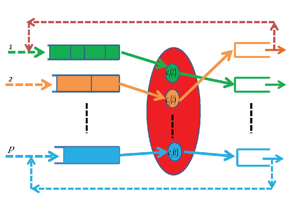
Refer to caption
Figure 4: A queueing network system with pp-job classes

whose dynamics (e.g., queue length process) is governed by specific forms of the FB-SDEs in (1). These forms can be a Lévy driven SDE, a pp-dimensional reflecting Brownian motion (RBM) (see, e.g., Dai [14], Dai and Dai [12], Dai and Jiang [21]), or a reflecting diffusion with regime switching (RDRS) (see, e.g., Dai [18]). The reflecting diffusion is the functional limit of a sequence of physical queueing processes under diffusive scaling, a general completely-𝒮{\cal S} boundary reflection constraint, and a well-known heavy traffic condition (an analogous treatment as the one for “infinite constant” in the KPZ equation (see, e.g., Hairer [26])). In reality, the characteristics of Lévy driven networks may be used to model or approximate more general batch-arrival and batch-service queueing networks. Second, we discuss how to use the queueing systems and their associated reflecting diffusion approximations to motivate the SDG problem. The criterion for the players in the game can be the queue length based performance optimization ones or queueing related cost/profit optimization ones. Third, we study the applications of the FB-SPDEs presented by (1) in the queueing networks. There are two types of equations involved. One is the Kolmogorov’s equation or Fokker-Planck’s formula oriented PDEs/SPDEs, which are corresponding to the distributions of queueing length processes under given network control rules. This type of equations are mainly used to estimate the performance measures of the queueing networks. Another type of equations are the HJB equation oriented PDES/SPDES, which are mainly used to obtain optimal control rules over the set of admissible strategies for the queueing networks.

The remainder of the paper is organized as follows. In Section 2, we introduce suitable functional topological space and state conditions required for our main theorems to guarantee the well-posedness of an adapted 4-tuple strong solution to the unified system of coupled FB-SPDEs in (1). In Section 3, we study the unified system of coupled FB-SDEs with Lévy jumps and skew reflections in (1) and present the well-posedness theorem. In particular, we establish the solution connection between the FB-SPDEs and the FB-SDEs. In Section 4, we formally formulate the FB-SDEs based SGE problem in (1.24) and determine the Pareto optimal Nash equilibrium policy process by a system of generalized stochastic HJB equations (a particular form of the coupled FB-SPDEs). Related applications in queueing networks are also discussed. Finally, in Sections 5-7, we develop theory to prove our main theorems.

2 The Unified System of Coupled FB-SPDEs with Lévy Jumps

First of all, let (Ω,ℱ,P)(\Omega,{\cal F},P) be a fixed complete probability space. Then, we define a standard dd-dimensional Brownian motion W≡{W⁡(t),t∈[0,T]}W\equiv\{W(t),t\in[0,T]\} for a given T∈[0,∞)T\in[0,\infty) with W⁡(t)=(W1​(t),…,Wd​(t))′W(t)=(W_{1}(t),...,W_{d}(t))^{\prime} and a hh-dimensional general Lévy pure jump process (or special subordinator) L≡{L⁡(t),t∈[0,T]}L\equiv\{L(t),t\in[0,T]\} with L⁡(t)≡(L1​(t),…,Lh​(t))′L(t)\equiv(L_{1}(t),...,L_{h}(t))^{\prime} on the space (see, e.g., Applebaum [1], Bertoin [6], and Sato [48]). Note that the prime appeared in this paper is used to denote the corresponding transpose of a matrix or a vector. Furthermore, WW, LL, and their components are supposed to be independent of each other. For each λ=(λ1,…​λh)′>0\lambda=(\lambda_{1},...\lambda_{h})^{\prime}>0, which is called a reversion rate vector in many applications, we let L⁡(λ​s)=(L1​(λ1​s),…,Lh​(λh​s))′L(\lambda s)=(L_{1}(\lambda_{1}s),...,L_{h}(\lambda_{h}s))^{\prime}. Then, we denote a filtration by {ℱt}t≥0\{{\cal F}_{t}\}_{t\geq 0} with ℱt≡σ{𝒢,W(s),L(λs):0≤s≤t}{\cal F}_{t}\equiv\sigma\{{\cal G},W(s),L(\lambda s):0\leq s\leq t\} for each t∈[0,T]t\in[0,T], where 𝒢{\cal G} is σ\sigma-algebra independent of WW and LL. In addition, let IA​(⋅)I_{A}(\cdot) be the index function over the set AA and νi\nu_{i} for each i∈{1,…,h}i\in\{1,...,h\} be a Lévy measure. Then, we use Ni​((0,t]×A)≡∑0<s≤tIA​(Li​(s)−Li​(s−))N_{i}((0,t]\times A)\equiv\sum_{0<s\leq t}I_{A}(L_{i}(s)-L_{i}(s^{-})) to denote a Poisson random measure with a deterministic, time-homogeneous intensity measure d​s​νi​(d​zi)ds\nu_{i}(dz_{i}). Thus, each LiL_{i} can be represented by (see, e.g., Theorem 13.4 and Corollary 13.7 in pages 237 and 239 of Kallenberg [30])

(2.26) Li​(t)=ai​(t)+∫(0,t]∫𝒵zi​Ni​(λi​𝑑s,d​zi),t≥0.\displaystyle L_{i}(t)=a_{i}(t)+\int_{(0,t]}\int_{{\cal Z}}z_{i}N_{i}(\lambda_{i}ds,dz_{i}),\;t\geq 0.

For convenience, we take the constant aia_{i} to be zero.

In the subsequent two subsections, we first study the unified system in (1), which is real-valued with a closed position parametric domain. Then, we extend the discussion to a complex-valued system with an open position parametric domain.

2.1 The Real-Valued System with Closed Position Parametric Domain

We let D∈RpD\in R^{p} be a closed position parametric domain and use Ck​(D,Rl)C^{k}(D,R^{l}) for each k∈𝒩k\in{\cal N} and l∈{r,q}l\in\{r,q\} to denote the Banach space of all functions ff having continuous derivatives up to the order kk with the uniform norm for each ff in this space,

(2.27) ‖f‖Ck​(D,l)=maxc∈{0,1,…,k}⁡max⁡supx∈Dj∈{1,…,r⁡(c)}⁡|fj(c)​(x)|.\displaystyle\|f\|_{C^{k}(D,l)}=\max_{c\in\{0,1,...,k\}}\max_{j\in\{1,...,r(c)\}}\sup_{x\in D}\left|f^{(c)}_{j}(x)\right|.

The r⁡(c)r(c) in (2.27) for each c∈{0,1,…,k}c\in\{0,1,...,k\} is the total number of the partial derivatives of the order cc

(2.28) fr,i1​…​ip(c)​(x)=∂cfr​(x)∂x1i1​…​∂xpip\displaystyle f^{(c)}_{r,i_{1}...i_{p}}(x)=\frac{\partial^{c}f_{r}(x)}{\partial x_{1}^{i_{1}}...\partial x_{p}^{i_{p}}}

with il∈{0,1,…,c}i_{l}\in\{0,1,...,c\}, l∈{1,…,p}l\in\{1,...,p\}, r∈{1,…,l}r\in\{1,...,l\}, and i1+…+ip=ci_{1}+...+i_{p}=c. Here, we remark that, whenever the partial derivative on the boundary ∂D{\partial D} is concerned, it is defined in a one-side manner. In addition, let

(2.29) fi1,…,ip(c)\displaystyle f_{i_{1},...,i_{p}}^{(c)} ≡\displaystyle\equiv (f1,i1,…,ip(c),…,fq,i1,…,ip(c)),\displaystyle(f_{1,i_{1},...,i_{p}}^{(c)},...,f_{q,i_{1},...,i_{p}}^{(c)}),
(2.30) f(c)​(x)\displaystyle f^{(c)}(x) ≡\displaystyle\equiv (f1(c)​(x),…,fr⁡(c)(c)​(x)),\displaystyle(f_{1}^{(c)}(x),...,f_{r(c)}^{(c)}(x)),

where each j∈{1,…,r⁡(c)}j\in\{1,...,r(c)\} corresponds to a pp-tuple (i1,…,ip)(i_{1},...,i_{p}) and a r∈{1,…,l}r\in\{1,...,l\}. Then, we use C∞​(D,Rl)C^{\infty}(D,R^{l}) to denote the Banach space

(2.31) C∞​(D,Rl)≡{f∈⋂c=0∞Cc​(D,Rl),‖f‖C∞​(D,l)<∞},\displaystyle C^{\infty}(D,R^{l})\equiv\left\{f\in\bigcap_{c=0}^{\infty}C^{c}(D,R^{l}),\|f\|_{C^{\infty}(D,l)}<\infty\right\},

where

(2.32) ‖f‖C∞​(D,q)2=∑c=0∞ξ⁡(c)​‖f‖Cc​(D,l)2\displaystyle\|f\|^{2}_{C^{\infty}(D,q)}=\sum_{c=0}^{\infty}\xi(c)\|f\|^{2}_{C^{c}(D,l)}

for some discrete function ξ⁡(c)\xi(c) in terms of c∈{0,1,2,…}c\in\{0,1,2,...\}, which is fast decaying in cc. For convenience, we take ξ⁡(c)=1((c10)!)​(η⁡(c)!)​ec\xi(c)=\frac{1}{((c^{10})!)(\eta(c)!)e^{c}} with

η⁡(c)=[max⁡{|x1|+…+|xp|,x∈D}]c,\displaystyle\eta(c)=[\max\{|x_{1}|+...+|x_{p}|,x\in D\}]^{c},

where the notation [][] denotes the summation of the unity and the integer part of a real number.

Next, let Lℱ2​([0,T],C∞​(D,Rl))L^{2}_{{\cal F}}([0,T],C^{\infty}(D;R^{l})) denote the set of all RlR^{l}-valued (or called C∞​(D,Rl)C^{\infty}(D;R^{l})-valued) measurable random vector-field processes Z⁡(t,x)Z(t,x) adapted to {ℱt,t∈[0,T]}\{{\cal F}_{t},t\in[0,T]\} for each x∈Dx\in D, which are in C∞​(D,Rl)C^{\infty}(D,R^{l}) for each fixed t∈[0,T]t\in[0,T]), such that

(2.33) E⁡[∫0T‖Z⁡(t)‖C∞​(D,l)2​𝑑t]<∞.\displaystyle E\left[\int_{0}^{T}\|Z(t)\|^{2}_{C^{\infty}(D,l)}dt\right]<\infty.

In particular, let L𝒢l2​(Ω,C∞​(D,Rl))L^{2}_{{\cal G}_{l}}(\Omega,C^{\infty}(D;R^{l})) with l∈{r,q}l\in\{r,q\} denote the set of all RlR^{l}-valued random vector-fields ζ⁡(x)\zeta(x) that are 𝒢l{\cal G}_{l}-measurable for each x∈Dx\in D and satisfy

(2.34) ‖ζ‖L𝒢2​(Ω,C∞​(D,Rl))2≡E⁡[‖ζ‖C∞​(D,l)2]<∞,\displaystyle\|\zeta\|^{2}_{L^{2}_{{\cal G}}(\Omega,C^{\infty}(D,R^{l}))}\equiv E\left[\|\zeta\|^{2}_{C^{\infty}(D,l)}\right]<\infty,

where 𝒢r=𝒢{\cal G}_{r}={\cal G} and 𝒢q=ℱT{\cal G}_{q}={\cal F}_{T}. In addition, let Lp2​([0,T]×𝒵hCLOSE,L^{2}_{p}([0,T]\times{\cal Z}^{h}, OPENC∞​(D,Rl×h))C^{\infty}(D,R^{l\times h})) be the set of all Rl×hR^{l\times h}-valued random vector-field processes denoted by V~​(t,x,z)=\tilde{V}(t,x,z)= (V~1​(t,x,z1)CLOSE,(\tilde{V}_{1}(t,x,z_{1}), ..., OPENV~h​(t,x,zh))\tilde{V}_{h}(t,x,z_{h})), which are predictable for each x∈Dx\in D and z∈𝒵hz\in{\cal Z}^{h} and are endowed with the norm

(2.35) E⁡[∑i=1h∫0T∫𝒵‖V~i​(t,zi)‖C∞​(D,l)2​νi​(d​zi)​𝑑t]<∞.\displaystyle E\left[\sum_{i=1}^{h}\int_{0}^{T}\int_{{\cal Z}}\left\|\tilde{V}_{i}(t,z_{i})\right\|^{2}_{C^{\infty}(D,l)}\nu_{i}(dz_{i})dt\right]<\infty.

Thus, we can define

(2.36) 𝒬ℱ2​([0,T]×D)\displaystyle{\cal Q}^{2}_{{\cal F}}([0,T]\times D) ≡\displaystyle\equiv Lℱ2​([0,T],C∞​(D,Rr))\displaystyle\;\;\;L^{2}_{{\cal F}}([0,T],C^{\infty}(D,R^{r}))
×Lℱ2​([0,T],C∞​(D,Rq))\displaystyle\times L^{2}_{{\cal F}}([0,T],C^{\infty}(D,R^{q}))
×Lℱ,p2​([0,T],C∞​(D,Rq×d))\displaystyle\times L^{2}_{{\cal F},p}([0,T],C^{\infty}(D,R^{q\times d}))
×Lp2​([0,T]×𝒵h,C∞​(D,Rq×h)).\displaystyle\times L^{2}_{p}([0,T]\times{\cal Z}^{h},C^{\infty}(D,R^{q\times h})).

Finally, let

(2.37) Lν2​(𝒵h,Cc​(D,Rq×h))\displaystyle L^{2}_{\nu}({\cal Z}^{h},C^{c}(D,R^{q\times h}))
≡{v~:𝒵h→Cc(D,Rq×h),∑i=1h∫𝒵‖v~i(zi)‖Cc​(D,q)2νi(dzi)<∞}\displaystyle\equiv\left\{\tilde{v}:{\cal Z}^{h}\rightarrow C^{c}(D,R^{q\times h}),\;\sum_{i=1}^{h}\int_{{\cal Z}}\left\|\tilde{v}_{i}(z_{i})\right\|^{2}_{C^{c}(D,q)}\nu_{i}(dz_{i})<\infty\right\}

that is endowed with the norm

(2.38) ‖v~‖ν,c2≡∑i=1h∫𝒵‖v~i​(zi)‖Cc​(D,q)2​λi​νi​(d​zi)\displaystyle\|\tilde{v}\|_{\nu,c}^{2}\equiv\sum_{i=1}^{h}\int_{{\cal Z}}\left\|\tilde{v}_{i}(z_{i})\right\|^{2}_{C^{c}(D,q)}\lambda_{i}\nu_{i}(dz_{i})

for any v~∈Lν2​(𝒵h,Cc​(D,Rq×h))\tilde{v}\in L^{2}_{\nu}({\cal Z}^{h},C^{c}(D,R^{q\times h})) and c∈{0,1,…,∞}c\in\{0,1,...,\infty\}. Furthermore, define

(2.39) 𝒱∞​(D)\displaystyle{\cal V}^{\infty}(D) ≡\displaystyle\equiv C∞​(D,Rr)\displaystyle C^{\infty}(D,R^{r})
×C∞​(D,Rq)\displaystyle\times C^{\infty}(D,R^{q})
×C∞​(D,Rq×d)\displaystyle\times C^{\infty}(D,R^{q\times d})
×L¯ν2​(𝒵h,C∞​(D,Rq×h)).\displaystyle\times\bar{L}^{2}_{\nu}({\cal Z}^{h},C^{\infty}(D,R^{q\times h})).

In the sequel, we let ‖A‖\|A\| be the largest absolute value of entries (or components) of the given matrix (or vector) AA. Furthermore, for each s∈[0,T]s\in[0,T] and z∈𝒵hz\in{\cal Z}^{h}, we let

(2.40) N~​(λ​d​s,d​z)\displaystyle\tilde{N}(\lambda ds,dz) =\displaystyle= (N~1​(λ1​d​s,d​z1),…,N~h​(λh​d​s,d​zh))′,\displaystyle(\tilde{N}_{1}(\lambda_{1}ds,dz_{1}),...,\tilde{N}_{h}(\lambda_{h}ds,dz_{h}))^{\prime},

where

(2.41) N~i​(λi​d​s,d​zi)=Ni​(λi​d​s,d​zi)−λi​d​s​νi​(d​zi)\displaystyle\tilde{N}_{i}(\lambda_{i}ds,dz_{i})=N_{i}(\lambda_{i}ds,dz_{i})-\lambda_{i}ds\nu_{i}(dz_{i})

for each i∈{1,…,h}i\in\{1,...,h\}. Then, we impose some conditions to guarantee the unique existence of an adapted 4-tuple strong solution to the unified system in (1).

First, for each 𝒜∈{ℒ,ℒ¯,𝒥,𝒥¯}{\cal A}\in\{{\cal L},\bar{\cal L},{\cal J},\bar{{\cal J}}\}, every c∈{0,1,2,…,}c\in\{0,1,2,...,\}, and any (ui,vi,v¯i,v~i)∈𝒱∞​(D)(u^{i},v^{i},\bar{v}^{i},\tilde{v}^{i})\in{\cal V}^{\infty}(D) with i∈{1,2}i\in\{1,2\}, we define

Δ​𝒜(c)​(s,x,u1,v1,v¯1,v~1,u2,v2,v¯2,v~2)\displaystyle\Delta{\cal A}^{(c)}(s,x,u^{1},v^{1},\bar{v}^{1},\tilde{v}^{1},u^{2},v^{2},\bar{v}^{2},\tilde{v}^{2})
≡𝒜(c)​(s,x,u1,v1,v¯1,v~1)−𝒜(c)​(s,x,u2,v2,v¯2,v~2).\displaystyle\equiv{\cal A}^{(c)}(s,x,u^{1},v^{1},\bar{v}^{1},\tilde{v}^{1})-{\cal A}^{(c)}(s,x,u^{2},v^{2},\bar{v}^{2},\tilde{v}^{2}).

Then, we assume that the generalized local Lipschitz condition is true almost surely (a.s.),

(2.42) ‖Δ​𝒜(c+l+o)​(s,x,u1,v1,v¯1,v~1,u2,v2,v¯2,v~2)‖\displaystyle\left\|\Delta{\cal A}^{(c+l+o)}(s,x,u^{1},v^{1},\bar{v}^{1},\tilde{v}^{1},u^{2},v^{2},\bar{v}^{2},\tilde{v}^{2})\right\|
≤KD,c​(‖u1−u2‖Ck+c​(D,r)+‖v1−v2‖Ck+c​(D,q)CLOSE\displaystyle\leq K_{D,c}\left(\|u^{1}-u^{2}\|_{C^{k+c}(D,r)}+\|v^{1}-v^{2}\|_{C^{k+c}(D,q)}\right.
OPEN+‖v¯1−v¯2‖Ck+c​(D,q​d)+‖v~1−v~2‖ν,k+c).\displaystyle\;\;\;\;\;\;\;\;\;\;\;\;\;\left.+\|\bar{v}^{1}-\bar{v}^{2}\|_{C^{k+c}(D,qd)}+\|\tilde{v}^{1}-\tilde{v}^{2}\|_{\nu,k+c}\right).

Note that KD,cK_{D,c} in (2.42) with each c∈{0,1,2,…}c\in\{0,1,2,...\} is a nonnegative constant. It depends on the domain DD and the differential order cc and may be unbounded as c→∞c\rightarrow\infty and D→RpD\rightarrow R^{p}. l∈{0,1,2}l\in\{0,1,2\} denotes the llth order of partial derivative of Δ​𝒜(c)​(s,x,u,v,v¯,v~)\Delta{\cal A}^{(c)}(s,x,u,v,\bar{v},\tilde{v}) in time variable tt. o∈{0,1,2}o\in\{0,1,2\} denotes the ooth order of partial derivative of Δ​𝒜(c+l)​(s,x,u,v,v¯,v~)\Delta{\cal A}^{(c+l)}(s,x,u,v,\bar{v},\tilde{v}) in terms of a component of uu, vv, v¯\bar{v}, or v~\tilde{v}. Furthermore, for each 𝒜∈{ℐ,ℐ¯}{\cal A}\in\{{\cal I},\bar{{\cal I}}\}, we suppose that

(2.43) ∑i=1h∫𝒵‖Δ​𝒜i(c+l+o)​(s,x,u1,v1,v¯1,v~1,u2,v2,v¯2,v~2,zi)‖2​λi​νi​(d​zi)\displaystyle\sum_{i=1}^{h}\int_{{\cal Z}}\left\|\Delta{\cal A}_{i}^{(c+l+o)}(s,x,u^{1},v^{1},\bar{v}^{1},\tilde{v}^{1},u^{2},v^{2},\bar{v}^{2},\tilde{v}^{2},z_{i})\right\|^{2}\lambda_{i}\nu_{i}(dz_{i})
≤KD,c​(‖u1−u2‖Ck+c​(D,r)2+‖v1−v2‖Ck+c​(D,q)2CLOSE\displaystyle\leq K_{D,c}\left(\|u^{1}-u^{2}\|^{2}_{C^{k+c}(D,r)}+\|v^{1}-v^{2}\|^{2}_{C^{k+c}(D,q)}\right.
OPEN+‖v¯1−v¯2‖Ck+c​(D,q​d)2+‖v~1−v~2‖ν,k+c2),\displaystyle\;\;\;\;\;\;\;\;\;\;\;\;\;\left.+\|\bar{v}^{1}-\bar{v}^{2}\|^{2}_{C^{k+c}(D,qd)}+\|\tilde{v}^{1}-\tilde{v}^{2}\|^{2}_{\nu,k+c}\right),

where 𝒜i{\cal A}_{i} is the iith column of 𝒜{\cal A}.

Second, for each 𝒜∈{ℒ,ℒ¯,𝒥,𝒥¯}{\cal A}\in\{{\cal L},\bar{\cal L},{\cal J},\bar{{\cal J}}\}, every c∈{0,1,2,…,}c\in\{0,1,2,...,\}, and any (u,v,v¯,v~)∈𝒱∞​(D)(u,v,\bar{v},\tilde{v})\in{\cal V}^{\infty}(D), we suppose that the generalized local linear growth condition holds

(2.44) ‖𝒜(c+l+o)​(s,x,u,v,v¯,v~)‖\displaystyle\left\|{\cal A}^{(c+l+o)}(s,x,u,v,\bar{v},\tilde{v})\right\|
≤KD,c​(δ0​c+‖u‖Ck+c​(D,r)+‖v‖Ck+c​(D,q)CLOSE\displaystyle\leq K_{D,c}\left(\delta_{0c}+\|u\|_{C^{k+c}(D,r)}+\|v\|_{C^{k+c}(D,q)}\right.
OPEN+‖v¯‖Ck+c​(D,q​d)+‖v~‖ν,k+c),\displaystyle\;\;\;\;\;\;\;\;\;\;\;\;\;\left.+\|\bar{v}\|_{C^{k+c}(D,qd)}+\|\tilde{v}\|_{\nu,k+c}\right),

where, δ0​c=1\delta_{0c}=1 if c=0c=0 and δ0​c=0\delta_{0c}=0 if c>0c>0. Similarly, for each 𝒜∈{ℐ,ℐ¯}{\cal A}\in\{{\cal I},\bar{{\cal I}}\}, we suppose that

(2.45) ∑i=1h∫𝒵‖𝒜i(c+l+o)​(s,x,u,v,v¯,v~,zi)‖2​λi​ν​(d​zi)\displaystyle\sum_{i=1}^{h}\int_{{\cal Z}}\left\|{\cal A}_{i}^{(c+l+o)}(s,x,u,v,\bar{v},\tilde{v},z_{i})\right\|^{2}\lambda_{i}\nu(dz_{i})
≤KD,c​(δ0​c+‖u‖Ck+c​(D,r)2+‖v‖Ck+c​(D,q)2CLOSE\displaystyle\leq K_{D,c}\left(\delta_{0c}+\|u\|^{2}_{C^{k+c}(D,r)}+\|v\|^{2}_{C^{k+c}(D,q)}\right.
OPEN+‖v¯‖Ck+c​(D,q​d)2+‖v~‖ν,k+c2).\displaystyle\;\;\;\;\;\;\;\;\;\;\;\;\;\left.+\|\bar{v}\|^{2}_{C^{k+c}(D,qd)}+\|\tilde{v}\|^{2}_{\nu,k+c}\right).

Then, we can state our main theorem of this subsection as follows.

Theorem 2.1

Suppose that (G,H)∈L𝒢2​(Ω,C∞​(D,Rr))×LℱT2​(Ω,C∞​(D,Rq))(G,H)\in L^{2}_{{\cal G}}(\Omega,C^{\infty}(D;R^{r}))\times L^{2}_{{\cal F}_{T}}(\Omega,C^{\infty}(D;R^{q})) and conditions in (2.42)-(2.45) are true. Furthermore, assume that each 𝒜∈{ℒ,ℒ¯,𝒥,𝒥¯,ℐ,ℐ¯}{\cal A}\in\{{\cal L},\bar{{\cal L}},{\cal J},\bar{{\cal J}},{\cal I},\bar{{\cal I}}\} is {ℱt}\{{\cal F}_{t}\}-adapted for every fixed x∈Dx\in D, z∈𝒵hz\in{\cal Z}^{h}, and any given (u,v,v¯,v~)∈𝒱∞​(D)(u,v,\bar{v},\tilde{v})\in{\cal V}^{\infty}(D) with

(2.46) ℒ⁡(⋅,x,0)∈Lℱ2​([0,T],C∞​(D,Rr)),\displaystyle{\cal L}(\cdot,x,0)\in L^{2}_{{\cal F}}\left([0,T],C^{\infty}(D,R^{r})\right),
(2.47) 𝒥⁡(⋅,x,0)∈Lℱ2​([0,T],C∞​(D,Rr×d)),\displaystyle{\cal J}(\cdot,x,0)\in L^{2}_{{\cal F}}\left([0,T],C^{\infty}(D,R^{r\times d})\right),
(2.48) ℐ⁡(⋅,x,0,⋅)∈Lℱ2​([0,T]×R+h,C∞​(D,Rr×h)),\displaystyle{\cal I}(\cdot,x,0,\cdot)\in L^{2}_{{\cal F}}\left([0,T]\times R_{+}^{h},C^{\infty}(D,R^{r\times h})\right),
(2.49) ℒ¯​(⋅,x,0)∈Lℱ2​([0,T],C∞​(D,Rq)),\displaystyle\bar{{\cal L}}(\cdot,x,0)\in L^{2}_{{\cal F}}\left([0,T],C^{\infty}(D,R^{q})\right),
(2.50) 𝒥¯​(⋅,x,0)∈Lℱ2​([0,T],C∞​(D,Rq×d)),\displaystyle\bar{{\cal J}}(\cdot,x,0)\in L^{2}_{{\cal F}}\left([0,T],C^{\infty}(D,R^{q\times d})\right),
(2.51) ℐ¯​(⋅,x,0,⋅)∈Lℱ2​([0,T]×R+h,C∞​(D,Rq×h)).\displaystyle\bar{{\cal I}}(\cdot,x,0,\cdot)\in L^{2}_{{\cal F}}\left([0,T]\times R_{+}^{h},C^{\infty}(D,R^{q\times h})\right).

Then, there exists a unique adapted 4-tuple strong solution to the system in (1), i.e.,

(2.52) (U,V,V¯,V~)∈𝒬ℱ2​([0,T]×D),\displaystyle(U,V,\bar{V},\tilde{V})\in{\cal Q}^{2}_{{\cal F}}([0,T]\times D),

and (U,V)​(⋅,x)(U,V)(\cdot,x) is càdlàg for each x∈Dx\in D almost surely (a.s.).

The proof of Theorem 2.1 is provided in Section 5.

2.2 The Complex-Valued System with Open Position Parametric Domain

In this subsection, we generalize the study in Subsection 2.1 to the case corresponding to an open (or partially open) position parametric domain DD (e.g., RpR^{p} or R+pR_{+}^{p}). More exactly, we assume that there exists a sequence of nondecreasing closed and connected sets {Dn,n∈{0,1,…}}\{D_{n},n\in\{0,1,...\}\} such that

(2.53) D=⋃n=0∞Dn.\displaystyle D=\bigcup_{n=0}^{\infty}D_{n}.

Furthermore, let C∞​(D,ℂl)C^{\infty}(D,\mathbb{C}^{l}) with l∈{r,q}l\in\{r,q\} be the Banach space endowed with the norm for each ff in the space

(2.54) ‖f‖C∞​(D,l)2≡∑n=0∞ξ⁡(n+1)​‖f‖C∞​(Dn,l)2,\displaystyle\|f\|^{2}_{C^{\infty}(D,l)}\equiv\sum_{n=0}^{\infty}\xi(n+1)\|f\|^{2}_{C^{\infty}(D_{n},l)},

where ℂl\mathbb{C}^{l} is the ll-dimensional complex Euclidean space and the norm ‖f‖C∞​(Dn,l)2\|f\|^{2}_{C^{\infty}(D_{n},l)} in (2.54) is interpreted in the corresponding complex-valued sense. In addition, define Q¯ℱ2​([0,τ]×D)\bar{Q}^{2}_{{\cal F}}([0,\tau]\times D) to be the corresponding space in (2.36) if the terminal time TT is replaced by the stopping time τ\tau in (1) and the norm in (2.32) is substituted by the one in (2.54). Finally, we use the same way to interpret the spaces L𝒢2​(Ω,C∞​(D,Rr))L^{2}_{{\cal G}}(\Omega,C^{\infty}(D;R^{r})) and Lℱτ2​(Ω,C∞​(D,Rq))L^{2}_{{\cal F}_{\tau}}(\Omega,C^{\infty}(D;R^{q})). Then, we have the following theorem.

Theorem 2.2

Suppose that (G,H)∈L𝒢2​(Ω,C∞​(D,Rr))×Lℱτ2​(Ω,C∞​(D,Rq))(G,H)\in L^{2}_{{\cal G}}(\Omega,C^{\infty}(D;R^{r}))\times L^{2}_{{\cal F}_{\tau}}(\Omega,C^{\infty}(D;R^{q})) and the system in (1) satisfies the conditions in (2.42)-(2.45) over DnD_{n} for each n∈{0,1,…}n\in\{0,1,...\} with associated (local) linear growth and Lipshitz constant KDn,cK_{D_{n},c}. Furthermore, assume that each 𝒜∈{ℒ,ℒ¯,𝒥,𝒥¯,ℐ,ℐ¯}{\cal A}\in\{{\cal L},\bar{{\cal L}},{\cal J},\bar{{\cal J}},{\cal I},\bar{{\cal I}}\} is {ℱt}\{{\cal F}_{t}\}-adapted for every fixed x∈Dx\in D, z∈𝒵hz\in{\cal Z}^{h}, and any given (u,v,v¯,v~)∈𝒱∞​(D)(u,v,\bar{v},\tilde{v})\in{\cal V}^{\infty}(D) with conditions in (2.46)-(2.51) being true. Then, the system in (1) has a unique adapted 4-tuple strong solution

(2.55) (U,V,V¯,V~)∈𝒬¯ℱ2​([0,τ]×D),\displaystyle(U,V,\bar{V},\tilde{V})\in\bar{{\cal Q}}^{2}_{{\cal F}}([0,\tau]\times D),

and (U,V)​(⋅,x)(U,V)(\cdot,x) is càdlàg for each x∈Dx\in D a.s.

The proof of Theorem 2.2 is provided in Section 5.

2.3 Illustrative Examples

In this subsection, we present two illustrative examples related to heat diffusions and quantum Hall/anomalous Hall effects. Mathematically, the heat diffusions are modeled as a stochastic Dirichlet-Poisson problem and the Hall effects are presented by a stochastic Schro¨\ddot{o}dinger equation. Examples related to queueing systems and SDGs will be presented in Section 4 after studying the system of coupled FB-SDEs in (1).

  • •

    Heat Diffusions: Stochastic Dirichlet-Poisson Problem

For this example, we consider a special B-SPDE (a specific backward part of the system in (1)). More precisely, the associated partial differential operators are given by

ℒ¯​(t,x,U,V,V¯,V~)\displaystyle\bar{{\cal L}}(t,x,U,V,\bar{V},\tilde{V}) ≡\displaystyle\equiv −g⁡(t,x)+12​∑j=1p∂2V⁡(t,x)∂xj2,\displaystyle-g(t,x)+\frac{1}{2}\sum_{j=1}^{p}\frac{\partial^{2}V(t,x)}{\partial x^{2}_{j}},
𝒥¯​(t,x,U,V,V¯,V~)\displaystyle\bar{{\cal J}}(t,x,U,V,\bar{V},\tilde{V}) ≡\displaystyle\equiv 0,\displaystyle 0,
ℐ¯​(t,x,U,V,V¯,V~,z)\displaystyle\bar{{\cal I}}(t,x,U,V,\bar{V},\tilde{V},z) ≡\displaystyle\equiv 0,\displaystyle 0,

where VV is single-dimensional (i.e., q=1q=1) and g⁡(t,x)g(t,x) is some integrable function. Then, we can obtain the corresponding B-SPDE with jumps as follows,

(2.56) V⁡(t,x)\displaystyle V(t,x) =\displaystyle= H⁡(x)+∫tτ(−g⁡(t,x)+12​∑j=1p∂2V⁡(t,x)∂xj2)​𝑑s\displaystyle H(x)+\int_{t}^{\tau}\left(-g(t,x)+\frac{1}{2}\sum_{j=1}^{p}\frac{\partial^{2}V(t,x)}{\partial x^{2}_{j}}\right)ds
−∫tτV¯(s,x)dW(s)\displaystyle\;\;\;\;\;\;\;\;\;-\int_{t}^{\tau}\bar{V}(s,x)dW(s)
−∫tτ∫z>0V~(s−,x,z)N~(λds,dz).\displaystyle\;\;\;\;\;\;\;\;\;-\int_{t}^{\tau}\int_{z>0}\tilde{V}(s^{-},x,z)\tilde{N}(\lambda ds,dz).

When the terminal value H⁡(x)H(x) is a boundary based condition over DD, we will call the related resolution problem a stochastic Dirichlet-Poisson problem with jumps, which is a randomized general form of the classical Dirichlet-Poisson problem (see, e.g., the definition of a classic case in ∅\emptysetksendal [39]). An explanation about how to use this problem to estimate the inner or surface temperature of certain material or an object (e.g., Sun) is displayed in Figure 5.

Refer to caption
Figure 5: A heat diffusion system by a solution to the Dirichlet-Poisson problem

Physically, the randomized heat equation in (2.56) is derived from a particle system just like its classic counterpart, which can be modeled by a diffusion process as follows,

(2.57) d​Xt=b⁡(Xt)​d​t+σ⁡(Xt)​d​W​(t).\displaystyle dX_{t}=b(X_{t})dt+\sigma(X_{t})dW(t).

Now, we use τDx\tau_{D}^{x} to denote the first exit time (a stopping time) of the process XtX_{t} from the time-space domain [0,T]×D[0,T]\times D, i.e.,

(2.58) τDx=i​n​f​{t>0,(t,Xt)∉[0,T]×D},\displaystyle\tau_{D}^{x}=inf\{t>0,(t,X_{t})\notin[0,T]\times D\},

where the upper index xx means that XtX_{t} starts from x∈Dx\in D. Then, we can impose a terminal-boundary condition with τ=τDx\tau=\tau_{D}^{x} as follows,

(2.59) limt→τDx​(ω)V⁡(t,Xt)=H⁡(τDx​(ω))=HD​(x,ω)a.s.Qx\displaystyle\lim_{t\rightarrow\tau_{D}^{x}(\omega)}V(t,X_{t})=H(\tau_{D}^{x}(\omega))=H_{D}(x,\omega)\;\;\;\;\;a.s.\;\;Q^{x}

for all (t,x)∈[0,T]×D(t,x)\in[0,T]\times D. In the case that HD​(x,ω)H_{D}(x,\omega) is a random variable independent of xx, the required smooth condition for the well-posedness of the B-SPDE in (2.56) is satisfied. In general, HD​(x,ω)H_{D}(x,\omega) can be approximated by sufficiently smooth function in xx as required.

  • •

    Hall Effects: Stochastic Schro¨\ddot{o}dinger Equation

In quantum physics and statistical mechanics, some phenomena such as Hall/anomalous Hall effects (see, e.g., Hall [25], Karplus and Luttinger [32], and the summarized description at Wikipedia website) are major concerns. By the definition of Hall effect, the movements of quantum particles (e.g., electrons) within a semiconduct/superconduct are along regular paths (see Figure 6 for such an example) if the Lorentz force generated by an external magnetic field with a perpendicular component is imposed.

Refer to caption
Figure 6: Edge states carry the current

When this phenomenon happens, the collisions of quantum particles will be significantly reduced and the performance of the semiconduct/superconduct will be largely improved. However, in a real application, imposing an external magnetic field is frequently expensive. Thus, people try to develop some magnetic material based semiconduct/superconduct in order that the Hall effect happens naturally (see, e.g., Karplus and Luttinger [32], Chang et al. [10]). This phenomenon is called anomalous Hall effect.

Besides observing the Hall/anomalous Hall effects by physical experiments (see, e.g., Hall [25] and Chang et al. [10]), one can also analytically study and simulate these effects through a Schro¨\ddot{o}dinger equation (see, e.g., Thouless [51], Chai [8, 9], and the summarized descriptions about density functional theory and time-dependent density functional theory at Wikipedia website). The Schro¨\ddot{o}dinger equation used in most existing studies is a form of the Fokker-Planck’s formula (see, e.g., ∅\emptysetksendal [39]). Here, by taking a form of ℒ{\cal L} in the forward part of the system in (1), we can unify these Schro¨\ddot{o}dinger equations (see, e.g., Bouard and Debussche [4, 5], Thouless [51], Chai [8, 9]) into the generalized stochastic nonlinear Schro¨\ddot{o}dinger equation with absorbing boundaries for each i∈{1,…,2​p}i\in\{1,...,2p\}),

(2.60) i​𝑑V​(t,x)=ℒ⁡(t−,x,V)​𝑑t+𝒥⁡(t−,x,V)​𝑑W​(t)+∫z>0ℐ⁡(t−,x,V,z)​N~​(λ​𝑑t,𝑑z),\displaystyle idV(t,x)={\cal L}(t^{-},x,V)dt+{\cal J}(t^{-},x,V)dW(t)+\int_{z>0}{\cal I}(t^{-},x,V,z)\tilde{N}(\lambda dt,dz),

where VV is single-dimensional (i.e., q=1q=1), ii is the imaginary number, and ℒ{\cal L} is a form of the operator,

(2.61) ℒ(t,x,V,⋅)\displaystyle{\cal L}(t,x,V,\cdot) =\displaystyle= ∑j=1paj​j​(x)​∂2V⁡(t,x)∂xj2+∑j=1pbj​(x)​∂V⁡(t,x)∂xj+c⁡(x,V)​V​(t,x).\displaystyle\sum_{j=1}^{p}a_{jj}(x)\frac{\partial^{2}V(t,x)}{\partial x_{j}^{2}}+\sum_{j=1}^{p}b_{j}(x)\frac{\partial V(t,x)}{\partial x_{j}}+c(x,V)V(t,x).

Note that c⁡(x,V)c(x,V) in (2.61) is the potential, which may depend on external temperature and/or external magnetic field. For example, the recent discovery about the Anomalous Hall Effect (see, e.g., Chang et al. [10]) is based on a lower temperature and without imposing external magnetic field. Furthermore, the related Schro¨\ddot{o}dinger equation based studies can be found in Chai [8, 9], etc.

Now, if the densities appeared in the Hall/Anomalous Hall Effects are the target stationary distributions (i.e., the terminal values H⁡(T,x)H(T,x) in (1) are given), we can take ℒ¯\bar{{\cal L}} in the system of (1) to be a form of the operator in (2.61). Then, we can find the initial and transient distributions of quantum particles by the backward part of the system in (1). From physical viewpoint, this study provides insights about how to characterize and manufacture the magnetic material based semiconductor/superconduct.

3 The Coupled FB-SDEs with Lévy Jumps and Skew Reflections

3.1 The Coupled FB-SDEs and Its Well-Posedness

In this section, we suppose that the process XX governed by the forward SDE in (1) lives in a state space DD (e.g., a pp-dimensional positive orthant or a pp-dimensional rectangle). Furthermore, let Di={x∈Rp,x⋅ni=bi}D_{i}=\{x\in R^{p},x\cdot n_{i}=b_{i}\} for i∈{1,…,b}i\in\{1,...,b\} be the iith boundary face of DD, where bi=0b_{i}=0 for i∈{1,…,p}i\in\{1,...,p\}, bib_{i} is some positive constant for i∈{p+1,…,b}i\in\{p+1,...,b\}, and nin_{i} is the inward unit normal vector on the boundary face DiD_{i}. For convenience, we define N=(n1,…,nb)N=(n_{1},...,n_{b}). In addition, let RR in (1) be a p×bp\times b matrix with b∈{p,2​p}b\in\{p,2p\}, whose iith column denoted by pp-dimensional vector viv_{i} is the reflection direction of XX on DiD_{i}. The process YY in (1) is a nondecreasing predictable process with Y⁡(0)=0Y(0)=0 and boundary regulating property as explained in (1). In queueing system, this process is called boundary idle time or blocking process.

Similarly, we assume that VV takes value in a region D¯\bar{D} with boundary face D¯i={v∈Rq,v⋅n¯i=b¯i}\bar{D}_{i}=\{v\in R^{q},v\cdot\bar{n}_{i}=\bar{b}_{i}\} for i∈{1,…,b¯}i\in\{1,...,\bar{b}\}, where n¯i\bar{n}_{i} is the inward unit normal vector on the boundary face D¯i\bar{D}_{i}. For convenience, we define N¯=(n¯1,…,n¯b¯)\bar{N}=(\bar{n}_{1},...,\bar{n}_{\bar{b}}). In finance, the given constant b¯i\bar{b}_{i} is called early exercise reward. Furthermore, SS in (1) is supposed to be a q×b¯q\times\bar{b} matrix for a known b¯∈{q,2​q}\bar{b}\in\{q,2q\}. In addition, F⁡(⋅)F(\cdot) in (1) is a nondecreasing predictable process with F⁡(0)=0F(0)=0 and boundary regulating property as explained in (1).

To guarantee the existence and uniqueness of an adapted 6-tuple weak solution to the coupled FB-SDEs in (1), we need to introduce the completely-𝒮{\cal S} condition on the reflection matrix RR (and similarly on SS).

Definition 3.1

A p×pp\times p square matrix RR is called completely-𝒮{\cal S} if and only if there is x>0x>0 such that R~​x>0\tilde{R}x>0 for each principal sub-matrix R~\tilde{R} of RR, where the vector inequalities are to be interpreted componentwise. Furthermore, a p×bp\times b matrix RR is called completely-𝒮{\cal S} if and only if each p×pp\times p square sub-matrix of N′​RN^{\prime}R is completely-S.

Note that the completely-𝒮{\cal S} condition on the reflection matrices guarantees that the coupled FB-SDEs are of inward reflection on each boundary and corner of the orthant or the rectangle (see, e.g., Figure 2 and Dai [14]). Furthermore, the reflection appeared here is called skew reflection that is a generalization of the conventional mirror (or called symmetry) reflection.

Now, the coefficient functions given in (1) are assumed to be {ℱt}\{{\cal F}_{t}\}-predictable and are detailed as follows,

b(t,x,u)≡b(t,x,v,v¯,v~,u,⋅)\displaystyle b(t,x,u)\equiv b(t,x,v,\bar{v},\tilde{v},u,\cdot) :\displaystyle: [0,T]×Rp×Rq×Rq×d×Rq×h×U→Rp,\displaystyle[0,T]\times R^{p}\times R^{q}\times R^{q\times d}\times R^{q\times h}\times U\rightarrow R^{p},
σ(t,x,u)≡σ(t,x,v,v¯,v~,u,⋅)\displaystyle\sigma(t,x,u)\equiv\sigma(t,x,v,\bar{v},\tilde{v},u,\cdot) :\displaystyle: [0,T]×Rp×Rq×Rq×d×Rq×h×U→Rp×d,\displaystyle[0,T]\times R^{p}\times R^{q}\times R^{q\times d}\times R^{q\times h}\times U\rightarrow R^{p\times d},
η(t,x,u)≡η(t,x,v,v¯,v~,u,z,⋅)\displaystyle\eta(t,x,u)\equiv\eta(t,x,v,\bar{v},\tilde{v},u,z,\cdot) :\displaystyle: [0,T]×Rp×Rq×Rq×d×Rq×h×U×𝒵h→Rp×h,\displaystyle[0,T]\times R^{p}\times R^{q}\times R^{q\times d}\times R^{q\times h}\times U\times{\cal Z}^{h}\rightarrow R^{p\times h},
c(t,x,u)≡c(t,x,v,v¯,v~,u,⋅)\displaystyle c(t,x,u)\equiv c(t,x,v,\bar{v},\tilde{v},u,\cdot) :\displaystyle: [0,T]×Rp×Rq×Rq×d×Rq×h×U→Rq,\displaystyle[0,T]\times R^{p}\times R^{q}\times R^{q\times d}\times R^{q\times h}\times U\rightarrow R^{q},
α(t,x,u)≡σ(t,x,v,v¯,v~,u,⋅)\displaystyle\alpha(t,x,u)\equiv\sigma(t,x,v,\bar{v},\tilde{v},u,\cdot) :\displaystyle: [0,T]×Rp×Rq×Rq×d×Rq×h×U→Rq×d,\displaystyle[0,T]\times R^{p}\times R^{q}\times R^{q\times d}\times R^{q\times h}\times U\rightarrow R^{q\times d},
ζ(t,x,u)≡γ(t,x,v,v¯,v~,u,z,⋅)\displaystyle\zeta(t,x,u)\equiv\gamma(t,x,v,\bar{v},\tilde{v},u,z,\cdot) :\displaystyle: [0,T]×Rp×Rq×Rq×d×Rq×h×U×𝒵h→Rq×h.\displaystyle[0,T]\times R^{p}\times R^{q}\times R^{q\times d}\times R^{q\times h}\times U\times{\cal Z}^{h}\rightarrow R^{q\times h}.

For f,f1,f2∈{b,σ,c,α}f,f^{1},f^{2}\in\{b,\sigma,c,\alpha\}, we suppose that

(3.62) ‖f⁡(u)‖\displaystyle\left\|f(u)\right\| ≤\displaystyle\leq L⁡(t,ω)​(1+‖x‖+‖v‖+‖v¯‖+‖v~‖ν),\displaystyle L(t,\omega)\left(1+\left\|x\right\|+\|v\|+\|\bar{v}\|+\|\tilde{v}\|_{\nu}\right),
(3.63) ‖f2​(u)−f1​(u)‖\displaystyle\left\|f^{2}(u)-f^{1}(u)\right\| ≤\displaystyle\leq L⁡(t,ω)​(‖x2−x1‖+‖v2−v1‖CLOSE\displaystyle L(t,\omega)\left(\left\|x^{2}-x^{1}\right\|+\left\|v^{2}-v^{1}\right\|\right.
OPEN+‖v¯2−v¯1‖+‖v~2−v~1‖ν).\displaystyle\;\;\;\;\;\;\;\;\;\;\;\;\left.+\left\|\bar{v}^{2}-\bar{v}^{1}\right\|+\left\|\tilde{v}^{2}-\tilde{v}^{1}\right\|_{\nu}\right).

Furthermore, for each f,f1,f2∈{γ,ζ}f,f^{1},f^{2}\in\{\gamma,\zeta\} and z∈𝒵hz\in{\cal Z}^{h}, we suppose that

(3.64) ∑i=1h∫𝒵‖fi​(u,zi)‖2​λi​νi​(d​zi)\displaystyle\sum_{i=1}^{h}\int_{{\cal Z}}\left\|f_{i}(u,z_{i})\right\|^{2}\lambda_{i}\nu_{i}(dz_{i})
≤L2​(t,ω)​(1+‖x‖2+‖v‖2+‖v¯‖2+‖v~‖ν2),\displaystyle\leq L^{2}(t,\omega)\left(1+\left\|x\right\|^{2}+\|v\|^{2}+\|\bar{v}\|^{2}+\|\tilde{v}\|^{2}_{\nu}\right),

where fif_{i} is the iith column of ff, and

(3.65) ∑i=1h∫𝒵‖fi2​(u,zi)−fi1​(u,zi)‖2​λi​νi​(d​zi)\displaystyle\sum_{i=1}^{h}\int_{{\cal Z}}\left\|f^{2}_{i}(u,z_{i})-f^{1}_{i}(u,z_{i})\right\|^{2}\lambda_{i}\nu_{i}(dz_{i})
≤L2​(t,ω)​(‖x2−x1‖2+‖v2−v1‖2+‖v¯2−v¯1‖2+‖v~2−v~1‖ν2).\displaystyle\leq L^{2}(t,\omega)\left(\left\|x^{2}-x^{1}\right\|^{2}+\left\|v^{2}-v^{1}\right\|^{2}+\left\|\bar{v}^{2}-\bar{v}^{1}\right\|^{2}+\left\|\tilde{v}^{2}-\tilde{v}^{1}\right\|^{2}_{\nu}\right).

In addition, we assume that the terminal value H⁡(x)≡H⁡(x,⋅)H(x)\equiv H(x,\cdot) satisfies the condition,

(3.66) ‖H⁡(x)‖≤L⁡(t,ω)​(1+‖x‖).\displaystyle\left\|H(x)\right\|\leq L(t,\omega)(1+\|x\|).

Finally, LL in (3.62)-(3.65) and (3.66) is assumed to be a known non-negative stochastic process that is {ℱt}\{{\cal F}_{t}\}-adapted and mean-squarely integrable, i.e.,

(3.67) E⁡[∫0TL2​(t)​𝑑t]<∞.\displaystyle E\left[\int_{0}^{T}L^{2}(t)dt\right]<\infty.
Theorem 3.1

Under conditions (3.62)-(3.67), the following two claims are true:

  1. 1.

    If SS and RR satisfy the completely-𝒮{\cal S} condition, there exists a unique adapted 6-tuple weak solution to the system in (1) when at least one of the forward and backward SDEs has reflection boundary;

  2. 2.

    Furthermore, if each q×qq\times q sub-principal matrix of N¯′​S\bar{N}^{\prime}S and each p×pp\times p sub-principal matrix of N′​RN^{\prime}R are invertible or if both of the SDEs have no reflection boundaries, there is a unique adapted 6-tuple strong solution to the system in (1).

Due to the length, the proof of Theorem 3.1 is postponed to Section 6.

3.2 Resolution via Coupled FB-SPDEs

In this subsection, we consider a particular case of the coupled FB-SPDEs in (1) but with an additional equation, which corresponds to the special forms of partial differential operators ℒ¯\bar{\cal L}, 𝒥¯\bar{\cal J}, and ℐ¯\bar{\cal I}. More precisely, for each l∈{0,1,…,q}l\in\{0,1,...,q\}, we define

(3.68) ℒ¯l​(t,x,U,V,V¯,V~,u)\displaystyle\bar{{\cal L}}_{l}(t,x,U,V,\bar{V},\tilde{V},u)
≡\displaystyle\equiv ∑i,j=1p(σ​σ′)i​j​(t,x,u)​∂2Vl​(t,x)∂xi​∂xj+∑i=1p(bi​(t,x,u)+∑j=1bvi​j​γj​(t,x))​∂Vl​(t,x)∂xi\displaystyle\sum_{i,j=1}^{p}(\sigma\sigma^{\prime})_{ij}(t,x,u)\frac{\partial^{2}V_{l}(t,x)}{\partial x_{i}\partial x_{j}}+\sum_{i=1}^{p}\left(b_{i}(t,x,u)+\sum_{j=1}^{b}v_{ij}\gamma_{j}(t,x)\right)\frac{\partial V_{l}(t,x)}{\partial x_{i}}
+∑j=1d∑i=1pσj​i(t,x,u)∂αl​j​(t,x,u)∂xi−cl(t,x,u)+∑k=1qsl​kβk(t,x)\displaystyle+\sum_{j=1}^{d}\sum_{i=1}^{p}\sigma_{ji}(t,x,u)\frac{\partial\alpha_{lj}(t,x,u)}{\partial x_{i}}-c_{l}(t,x,u)+\sum_{k=1}^{q}s_{lk}\beta_{k}(t,x)
−∑j=1h∫𝒵(Vl(t,x+ηj(t,x,u,zj))−Vl(t,x)−∑i=1p∂Vl​(t,x)∂xiηi​j(t,x,u,zj))νj(dzj)\displaystyle-\sum_{j=1}^{h}\int_{{\cal Z}}\left(V_{l}(t,x+\eta_{j}(t,x,u,z_{j}))-V_{l}(t,x)-\sum_{i=1}^{p}\frac{\partial V_{l}(t,x)}{\partial x_{i}}\eta_{ij}(t,x,u,z_{j})\right)\nu_{j}(dz_{j})
−∑j=1h∫𝒵(ζ~l​j(t,x+ηj(t,x,u,zj)),u,zj)−ζ~l​j(t,x,u,zj))νj(dzj),\displaystyle-\sum_{j=1}^{h}\int_{{\cal Z}}\left(\tilde{\zeta}_{lj}(t,x+\eta_{j}(t,x,u,z_{j})),u,z_{j})-\tilde{\zeta}_{lj}(t,x,u,z_{j})\right)\nu_{j}(dz_{j}),

where ηi​j\eta_{ij} and ηj\eta_{j} for i∈{1,…,p}i\in\{1,...,p\} and j∈{1,…,h}j\in\{1,...,h\} are the (i,j)(i,j)th entry and the jjth column of η\eta respectively. Furthermore,

(3.69) c0​(t,x,u)\displaystyle c_{0}(t,x,u) =\displaystyle= ∑l=1qcl​(t,x,u),\displaystyle\sum_{l=1}^{q}c_{l}(t,x,u),
(3.70) OPENζ~0​j​(t,x,u,zj))\displaystyle\tilde{\zeta}_{0j}(t,x,u,z_{j})) =\displaystyle= OPEN∑l=1qζl​j​(t,x,u,zj)),\displaystyle\sum_{l=1}^{q}\zeta_{lj}(t,x,u,z_{j})),

and ζl​j\zeta_{lj} for l∈{1,…,q}l\in\{1,...,q\} and j∈{1,…,h}j\in\{1,...,h\} is the (i,j)(i,j)th entry of ζ\zeta. In addition, γj​(t,x)\gamma_{j}(t,x) for j∈{1,…,b}j\in\{1,...,b\} and βk​(t,x)\beta_{k}(t,x) for k∈{1,…,q}k\in\{1,...,q\} are some functions in tt and xx.

Note that, the partial derivative

∂αl​j​(t,x,u)∂xifor eachl∈{0,1,…,q},i∈{1,…,p},j∈{1,…,d}\displaystyle\frac{\partial\alpha_{lj}(t,x,u)}{\partial x_{i}}\;\;\mbox{for each}\;\;l\in\{0,1,...,q\},\;i\in\{1,...,p\},\;j\in\{1,...,d\}

should be interpreted according to chain rule since α⁡(t,x)\alpha(t,x) is also a function in xx through (V,V¯,V~)​(t,x)(V,\bar{V},\tilde{V})(t,x) and u⁡(t,x)u(t,x), where

(3.71) α0​j​(t,x,u)=∑l=1qαl​j​(t,x,u).\displaystyle\alpha_{0j}(t,x,u)=\sum_{l=1}^{q}\alpha_{lj}(t,x,u).

Finally, we define

(3.72) 𝒥¯​(t,x,U,V,V¯,V~)\displaystyle\bar{{\cal J}}(t,x,U,V,\bar{V},\tilde{V}) =\displaystyle= −V¯​(t,x),\displaystyle-\bar{V}(t,x),
(3.73) ℐ¯​(t,x,U,V,V¯,V~,z)\displaystyle\bar{{\cal I}}(t,x,U,V,\bar{V},\tilde{V},z) =\displaystyle= −V~​(t,x),\displaystyle-\tilde{V}(t,x),
(3.74) V⁡(T,x)\displaystyle V(T,x) =\displaystyle= H⁡(x),\displaystyle H(x),

where, we assume that H∈LℱT2​(Ω,C∞​(D,Rq))H\in L^{2}_{{\cal F}_{T}}(\Omega,C^{\infty}(D;R^{q})). Then, we have the following definition.

Definition 3.2

𝒞{\cal C} is called the admissible set of adapted control processes if {ℒ¯l(t,x,U,V\{\bar{{\cal L}}_{l}(t,x,U,V, V¯,V~,u),l∈{0,1,…,q}}\bar{V},\tilde{V},u),l\in\{0,1,...,q\}\} together with {ℒ,𝒥,ℐ,𝒥¯,ℐ¯}\{{\cal L},{\cal J},{\cal I},\bar{{\cal J}},\bar{{\cal I}}\} satisfy the conditions as stated in Theorem 2.1 (or Theorem 2.2).

Theorem 3.2

Let (U(t,x),V(t,x),V¯(t,x),V~(t,x,⋅))(U(t,x),V(t,x),\bar{V}(t,x),\tilde{V}(t,x,\cdot)) be the unique adapted 4-tuple strong solution to the (r,q+1)(r,q+1)-dimensional coupled FB-SPDEs in (1), which corresponds to specific {ℒ¯,𝒥¯,ℐ¯}\{\bar{{\cal L}},\bar{{\cal J}},\bar{{\cal I}}\} in (3.68)-(3.73), terminal condition in (3.74), and a control process u∈𝒞u\in{\cal C}. If SS and RR satisfy the completely-𝒮{\cal S} condition, the following claims in are true:

  1. 1.

    There exists a unique adapted 6-tuple weak solution ((X⁡(t),Y⁡(t))CLOSE((X(t),Y(t)), OPEN(V⁡(t),V¯​(t),V~​(t,z),F⁡(t)))(V(t),\bar{V}(t),\tilde{V}(t,z),F(t))) to the system in (1) when at least one of the SDEs has reflection boundary, where

    (3.75) Vl​(t)\displaystyle V_{l}(t) =\displaystyle= Vl​(t,X​(t)),\displaystyle V_{l}(t,X(t)),
    (3.76) V¯l​j​(t)\displaystyle\bar{V}_{lj}(t) =\displaystyle= −(αl​j​(t,X⁡(t),u)+∑i=1pσl​i​(t,X⁡(t),u)​∂Vl​(t,X⁡(t))∂xi),\displaystyle-\left(\alpha_{lj}(t,X(t),u)+\sum_{i=1}^{p}\sigma_{li}(t,X(t),u)\frac{\partial V_{l}(t,X(t))}{\partial x_{i}}\right),
    (3.77) OPENV~l​j​(t,z))\displaystyle\tilde{V}_{lj}(t,z)) =\displaystyle= −(Vl​(t,X⁡(t)+ηj​(t,X⁡(t),u,zj))−Vl​(t,X⁡(t)))\displaystyle-\left(V_{l}(t,X(t)+\eta_{j}(t,X(t),u,z_{j}))-V_{l}(t,X(t))\right)
    −ζl​j​(t,X⁡(t)+ηj​(t,X⁡(t),u,zj),u,zj)\displaystyle-\zeta_{lj}(t,X(t)+\eta_{j}(t,X(t),u,z_{j}),u,z_{j})

    for l∈{0,1,…,q}l\in\{0,1,...,q\} and j∈{1,…,h}j\in\{1,...,h\}, where

    (3.78) α⁡(t,X⁡(t),u)\displaystyle\;\;\;\;\;\;\;\;\alpha(t,X(t),u) =\displaystyle= α(t,X(t),V(t,X(t)),V¯(t,X(t)),V~(t,X(t),⋅),u(t,X(t)),⋅),\displaystyle\alpha(t,X(t),V(t,X(t)),\bar{V}(t,X(t)),\tilde{V}(t,X(t),\cdot),u(t,X(t)),\cdot),
    (3.79) η⁡(t,X⁡(t),u)\displaystyle\;\;\;\;\;\;\;\;\eta(t,X(t),u) =\displaystyle= η(t,X(t),V(t,X(t)),V¯(t,X(t)),V~(t,X(t),⋅),u(t,X(t)),⋅),\displaystyle\eta(t,X(t),V(t,X(t)),\bar{V}(t,X(t)),\tilde{V}(t,X(t),\cdot),u(t,X(t)),\cdot),
    (3.80) ζ⁡(t,X⁡(t),u)\displaystyle\;\;\;\;\;\;\;\;\zeta(t,X(t),u) =\displaystyle= ζ(t,X(t),V(t,X(t)),V¯(t,X(t)),V~(t,X(t),⋅),u(t,X(t)),⋅);\displaystyle\zeta(t,X(t),V(t,X(t)),\bar{V}(t,X(t)),\tilde{V}(t,X(t),\cdot),u(t,X(t)),\cdot);
  2. 2.

    There is a unique adapted 6-tuple strong solution to the system in (1) when each q×qq\times q sub-principal matrix of N¯′​S\bar{N}^{\prime}S and each p×pp\times p sub-principal matrix of N′​RN^{\prime}R are invertible or when both of the SDEs have no reflection boundaries.

4 Connections to Non-Zero-Sum SDGs and Queues

4.1 Non-Zero-Sum SDGs

By Theorem 3.2, we suppose that the 44-tuple (X,V,V¯,V~)(X,V,\bar{V},\tilde{V}) in (4.1) is part of a solution (X,Y,V,V¯,V~,F)(X,Y,V,\bar{V},\tilde{V},F) to the non-Markvian system of coupled FB-SDEs with Lévy jumps and skew reflections in (1). Then, let u⁡(⋅)u(\cdot) be the corresponding BB-valued (B⊂RqB\subset R^{q}) and {ℱt}\{{\cal F}_{t}\}-adapted control process, whose llth component ul​(⋅)u_{l}(\cdot) for each l∈{1,…,q}l\in\{1,...,q\} is the llth player’s control policy. Furthermore, we assume that the utility function for each player l∈{1,…,q}l\in\{1,...,q\} is defined by

{cl​(t,X​(t),u)≡cl​(t,X⁡(t),V⁡(t,X⁡(t)),V¯​(t,X⁡(t)),V~​(t,X⁡(t)),u⁡(t,X⁡(t))),c0​(t,X​(t),u)≡∑l=1qcl​(t,X⁡(t),u),\displaystyle\left\{\begin{array}[]{ll}c_{l}(t,X(t),u)&\equiv c_{l}(t,X(t),V(t,X(t)),\bar{V}(t,X(t)),\tilde{V}(t,X(t)),u(t,X(t))),\\ c_{0}(t,X(t),u)&\equiv\sum_{l=1}^{q}c_{l}(t,X(t),u),\end{array}\right.

Thus, it follows from (3.79)-(3.80), (3.70)-(3.71), and (4.1) that the value functions {Vlu​(0),l∈{1,…,q}}\{V^{u}_{l}(0),l\in\{1,...,q\}\} in (1.24) are now well defined. Then, we can introduce the following concepts.

Definition 4.1

By a non-zero-sum SDG to the system in (1), we mean that each player l∈{1,…,q}l\in\{1,...,q\} chooses an optimal policy to maximize his own value function expressed in (1.24). Furthermore, the value functions {Vlu​(0),l∈{1,…,q}}\{V^{u}_{l}(0),l\in\{1,...,q\}\} do not have to add up to a constant (e.g., zero), or in other words, the SDG is not necessarily a zero-sum one.

Definition 4.2

u∗​(⋅)u^{*}(\cdot) is called a Pareto optimal Nash equilibrium policy process if, the process is also an optimal one to the sum of all the qq players’ value functions at time zero; no player will profit by unilaterally changing his own policy when all the other players’ policies keep the same. Mathematically,

(4.84) V0u∗​(0)≥V0u​(0),Vlu∗​(0)≥Vlu−l∗​(0)\displaystyle V_{0}^{u^{*}}(0)\geq V_{0}^{u}(0),\;\;\;V_{l}^{u^{*}}(0)\geq V_{l}^{u^{*}_{-l}}(0)

for each l∈{0,1,…,q}l\in\{0,1,...,q\} and any given admissible control policy uu, where

u−l∗=(u1∗,…,ul−1∗,ul,ul+1∗,…,uq∗).\displaystyle u^{*}_{-l}=(u_{1}^{*},...,u^{*}_{l-1},u_{l},u^{*}_{l+1},...,u^{*}_{q}).
Definition 4.3

{ℒ¯l​(t,x,U,V,V¯,V~,u),l∈{0,1,…,q}}\{\bar{{\cal L}}_{l}(t,x,U,V,\bar{V},\tilde{V},u),l\in\{0,1,...,q\}\} together with {ℒ,𝒥,ℐ}\{{\cal L},{\cal J},{\cal I}\} are called satisfying the comparison principle in terms of uu if, for any two ui∈𝒞u^{i}\in{\cal C} with i∈{1,2}i\in\{1,2\} and any two ℱT{\cal F}_{T}-measurable HiH^{i} with associated two solutions (Ui,Vi,V¯i,V~i)​(t,x)(U^{i},V^{i},\bar{V}^{i},\tilde{V}^{i})(t,x), respectively, of (1) such that

ℒ¯l​(t,x,U1,V1,V¯1,V~1,u1)\displaystyle\bar{{\cal L}}_{l}(t,x,U^{1},V^{1},\bar{V}^{1},\tilde{V}^{1},u^{1}) ≤\displaystyle\leq ℒ¯l​(t,x,U2,V2,V¯2,V~2,u2),\displaystyle\bar{{\cal L}}_{l}(t,x,U^{2},V^{2},\bar{V}^{2},\tilde{V}^{2},u^{2}),
H1​(x)\displaystyle H^{1}(x) ≤\displaystyle\leq H2​(x)\displaystyle H^{2}(x)

for all (t,x)∈[0,T]×D(t,x)\in[0,T]\times D, we have

V1​(t,x)≤V2​(t,x).\displaystyle V^{1}(t,x)\leq V^{2}(t,x).
Theorem 4.1

Let (U(t,x),V(t,x),V¯(t,x),V~(t,x,⋅))(U(t,x),V(t,x),\bar{V}(t,x),\tilde{V}(t,x,\cdot)) be the unique adapted 4-tuple strong solution to the (r,q+1)(r,q+1)-dimensional FB-SPDEs in (1), which corresponds to specific {ℒ¯,𝒥¯,ℐ¯}\{\bar{{\cal L}},\bar{{\cal J}},\bar{{\cal I}}\} in (3.68)-(3.73), terminal condition in (3.74), and a control process u∈𝒞u\in{\cal C}. Suppose that SS and RR satisfy the completely-𝒮{\cal S} condition. If {ℒ¯l​(t,x,U,V,V¯,V~,u),l∈{0,1,…,q}}\{\bar{{\cal L}}_{l}(t,x,U,V,\bar{V},\tilde{V},u),l\in\{0,1,...,q\}\} together with {ℒ,𝒥,ℐ,𝒥¯,ℐ¯}\{{\cal L},{\cal J},{\cal I},\bar{{\cal J}},\bar{{\cal I}}\} for suitably chosen γ⁡(t,x)\gamma(t,x) and β⁡(t,x)\beta(t,x) satisfy the comparison principle in terms of uu, the following two claims are true:

  1. 1.

    There is a Pareto optimal Nash equilibrium point u∗​(t,X​(t))u^{*}(t,X(t)) to the non-zero-sum SDG problem in (1.24) when both of the SDEs in (1) have no reflection boundaries and if γ⁡(t,x)=β⁡(t,x)≡0\gamma(t,x)=\beta(t,x)\equiv 0;

  2. 2.

    There is an approximated Pareto optimal Nash equilibrium point u∗​(t,X​(t))u^{*}(t,X(t)) to the non-zero-sum SDG problem in (1.24) when at least one of the SDEs in (1) has reflection boundary and if γ⁡(t,x)\gamma(t,x), β⁡(t,x)\beta(t,x) are taken to be infinitely smooth approximated functions of d​Fd​t\frac{dF}{dt}(t,x) and d​Yd​t​(t,x)\frac{dY}{dt}(t,x) in xx.

4.2 Queues and Reflecting Diffusions

Queueing networks widely appear in real-world applications such as those in service, cloud computing, and communication systems. They typically consist of arrival processes, service processes, and buffer storages with certain kind of service regime and network architecture (see, e.g., an example with pp-job classes in Figure 4). The major performance measure for this system is the queue length process denoted by Q⁡(⋅)=(Q1​(⋅),…,Qp​(⋅))′Q(\cdot)=(Q_{1}(\cdot),...,Q_{p}(\cdot))^{\prime}, where Qi​(t)Q_{i}(t) is the number of iith class jobs stored in the iith buffer for each i∈{1,…,p}i\in\{1,...,p\} at time tt. Let Q⁡(0)Q(0) be the initial queue length for the system. Then, the queueing dynamics of the system can be presented by

(4.85) Q⁡(t)=Q⁡(0)+A⁡(t)−D⁡(t),\displaystyle Q(t)=Q(0)+A(t)-D(t),

where, the iith component Ai​(t)A_{i}(t) of A⁡(t)A(t) for each i∈{1,…,p}i\in\{1,...,p\} is the total number of jobs arrived to buffer ii by time tt, and the iith component Di​(t)D_{i}(t) of D⁡(t)D(t) is the total number of jobs departed from buffer ii by time tt. In the following discussions, we use two generalized ways to characterize the arrival and departure processes.

First, we assume that each Ai​(⋅)A_{i}(\cdot) for i∈{1,…,p}i\in\{1,...,p\} is a time-inhomogeneous Lévy process with intensity measure ai​(t,Q⁡(t),zi)​d​t​νi​(d​zi)a_{i}(t,Q(t),z_{i})dt\nu_{i}(dz_{i}) that is the job arrival rate to buffer ii at time tt and depends on the queue state at time tt. Similarly, we assume that each Di​(⋅)D_{i}(\cdot) is also a time-inhomogeneous Lévy process with intensity measure di​(t,Q⁡(t),zi)​d​t​νi​(d​zi)d_{i}(t,Q(t),z_{i})dt\nu_{i}(dz_{i}) that is the assigned service rate to buffer ii at time tt. Furthermore, we assume that the routing proportion from buffer jj to buffer ii for jobs finishing service at buffer jj is pj​i​(t,Q⁡(t),zj)p_{ji}(t,Q(t),z_{j}). Then, by the F-SDE in (1) and the discussions in Applebaum [1], the queue length process in (4.85) for this case can be further expressed by

(4.86) d​Qi​(t)\displaystyle dQ_{i}(t) =\displaystyle= (∫𝒵ai​(t,Q⁡(t),zi)​νi​(d​zi)CLOSE\displaystyle\left(\int_{{\cal Z}}a_{i}(t,Q(t),z_{i})\nu_{i}(dz_{i})\right.
+∑j≠i∫𝒵pj​i(t,Q(t),zj)dj(t,Q(t),zj)I{Qj(t)>0}νj(dzj)\displaystyle+\sum_{j\neq i}\int_{{\cal Z}}p_{ji}(t,Q(t),z_{j})d_{j}(t,Q(t),z_{j})I_{\{Q_{j}(t)>0\}}\nu_{j}(dz_{j})
−∫𝒵di(t,Q(t),zi)I{Qi(t)>0}νi(dzi))dt\displaystyle\left.-\int_{{\cal Z}}d_{i}(t,Q(t),z_{i})I_{\{Q_{i}(t)>0\}}\nu_{i}(dz_{i})\right)dt
+∫𝒵ai(t,Q(t),zi)N~i(dt,dzi)\displaystyle+\int_{{\cal Z}}a_{i}(t,Q(t),z_{i})\tilde{N}_{i}(dt,dz_{i})
+∑j≠i∫𝒵pj​i(t,Q(t),zj)dj(t,Q(t),zj)I{Qj(t)>0}N~j(dt,dzj)\displaystyle+\sum_{j\neq i}\int_{{\cal Z}}p_{ji}(t,Q(t),z_{j})d_{j}(t,Q(t),z_{j})I_{\{Q_{j}(t)>0\}}\tilde{N}_{j}(dt,dz_{j})
−∫𝒵di(t,Q(t),zi)I{Qi(t)>0}N~i(dt,dzi)\displaystyle-\int_{{\cal Z}}d_{i}(t,Q(t),z_{i})I_{\{Q_{i}(t)>0\}}\tilde{N}_{i}(dt,dz_{i})
+∑j=1bRi​j(t,Q(t))dYj(t),\displaystyle+\sum_{j=1}^{b}R_{ij}(t,Q(t))dY_{j}(t),

where, 𝒵=R+{\cal Z}=R_{+}, Yj​(t)Y_{j}(t) in (4.86) for each j∈{1,…,b}j\in\{1,...,b\} is the Skorohod regulator process and it can increase only at time tt when Qj​(t)=0Q_{j}(t)=0. Note that R⁡(t,Q⁡(t))R(t,Q(t)) is a reflection matrix that may be time and queue state dependent, and the coefficients in (4.86) may be discontinuous at the queue state Qi​(t)=0Q_{i}(t)=0. However, since the system in (4.86) is designed in a controllable manner, the service rate di​(s,Q​(s))d_{i}(s,Q(s)) can always be set to be zero when Qi​(t)=0Q_{i}(t)=0, which implies that the reflection part in (4.86) can be removed. Hence, the generalized Lipschitz and linear growth conditions in (3.62)-(3.65) may be reasonably imposed to the system in (4.86). Thus, the system derived in (4.86) can be well-posed. Furthermore, the optimal policies in terms of cost, profit, and system performance can be designed and analyzed (see, e.g., the related illustration in the coming Subsection 4.3). Interested readers can also find some specific formulations of the queueing system (4.86) in Mandelbaum and Massey [36], Mandelbaum and Pats [37], and Konstantopoulos et al. [33], etc.

Second, we assume that both the arrival and service processes are described by renewal processes, renewal reward processes, or doubly stochastic renewal processes. In this case, the driven processes for the queueing system do not have the nice statistical properties such as memoryless and stationary increment ones. Thus, it is usually impossible to conduct exact analysis concerning the distribution of Q⁡(⋅)Q(\cdot). However, under certain conditions (e.g., the arrival rates close to the associated service rates), one can show that the corresponding sequence of diffusion-scaled queue length processes converges in distribution to a pp-dimensional reflecting Brownian motion (RBM) (see, e.g., Dai [14], Dai and Dai [12], Dai and Jiang [21]), or more generally, a reflecting diffusion with regime switching (RDRS) (see, e.g., Dai [18]). In other words, we have that

(4.87) Q^r(⋅)≡1rQ(r2⋅)⇒Q^(⋅)alongr∈{1,2,…},\displaystyle\hat{Q}^{r}(\cdot)\equiv\frac{1}{r}Q(r^{2}\cdot)\Rightarrow\hat{Q}(\cdot)\;\;\;\mbox{along}\;\;r\in\{1,2,...\},

where “⇒\Rightarrow” means “converges in distribution” and Q^​(⋅)\hat{Q}(\cdot) is a RBM or a RDRS.

To be simple, we consider the case that the limit Q^​(⋅)\hat{Q}(\cdot) in (4.87) is a RBM living in the state space DD introduced in Section 3. Furthermore, let θ\theta be a vector in RpR^{p} and Γ\Gamma be a p×pp\times p symmetric and positive definite matrix. Then, we can introduce the definition of a RBM (see, e.g, Dai [14]) as follows.

Definition 4.4

A semimartingale RBM associated with the data (𝐒,θ,Γ,R)({\bf S},\theta,\Gamma,R) that has initial distribution π\pi is a continuous, {ℱt}\{{\cal F}_{t}\}-adapted, pp-dimensional process ZZ defined on some filtered probability space (Ω,ℱ,{ℱt},𝐏)(\Omega,{\cal F},\{{\cal F}_{t}\},{\bf P}) such that under 𝐏{\bf P},

X⁡(t)=Z⁡(t)+R​Y​(t)​f​o​r​a​l​l​t≥0,\displaystyle X(t)=Z(t)+RY(t)\;\;for\;all\;t\geq 0,

where

  1. 1.

    XX has continuous paths in 𝐒{\bf S}, 𝐏{\bf P}-a.s.,

  2. 2.

    under 𝐏{\bf P}, ZZ is a pp-dimensional Brownian motion with drift vector θ\theta and covariance matrix Γ\Gamma such that {Z⁡(t)−θ​t,ℱt,t≥0}\{Z(t)-\theta t,{\cal F}_{t},t\geq 0\} is a martingale and P​Z−1​(0)=πP{Z}^{-1}(0)=\pi,

  3. 3.

    YY is a {ℱt}\{{\cal F}_{t}\}-adapted, bb-dimensional process such that 𝐏{\bf P}-a.s., for each i∈{1,…,b}i\in\{1,...,b\}, the iith component YiY_{i} of YY satisfies

    1. (a)

      Yi​(0)=0Y_{i}(0)=0,

    2. (b)

      YiY_{i} is continuous and non-decreasing,

    3. (c)

      YiY_{i} can increase only when Z is on the face DiD_{i}, i.e., as given in (1).

From the physical viewpoint of queueing system (see, e.g., Dai [14, 18]) and the discussion in Reiman and Williams [47], the pushing process YY in Definition 4.4 can be assumed to a.s. satisfy

(4.88) Yi​(t)=∫0tIDi​(X⁡(s))​𝑑s.\displaystyle Y_{i}(t)=\int_{0}^{t}I_{D_{i}}(X(s))ds.

Now, assume that H⁡(x)H(x) is the stationary distribution that we expect for the RBM XX. For example, in reality, it is the given distribution of the long-run average queue lengths among different users or job classes. Theoretically, it can be computed by a method (e.g., the finite element method designed and implemented in Dai et al. [14, 49]). Then, we can use a B-PDE or a B-SPDE (a special form of the system in (1)) to get the transition function at each time point to reach the targeted or limiting stationary distribution H⁡(x)H(x) for the RBM XX for a given initial distribution (e.g., X⁡(0)=0X(0)=0 a.s. in many situations). Hence, the corresponding performance measures of the physical queueing system can be estimated. More precisely, we have the following theorem and related remark.

Theorem 4.2

Suppose that the reflection matrix satisfies the completely-𝒮{\cal S} condition. Then, the transition function of the RBM XX over [0,T][0,T] is determined by

(4.89) V⁡(t,x)\displaystyle\;\;\;\;\;V(t,x) =\displaystyle= H⁡(x)+∫tTℒ⁡(s,x,V)​𝑑s,\displaystyle H(x)+\int_{t}^{T}{\cal L}(s,x,V)ds,

where VV is a 11-dimensional function. Furthermore, ℒ{\cal L} is the following form of partial differential operator

(4.90) ℒ(t,x,V,⋅)\displaystyle{\cal L}(t,x,V,\cdot) =\displaystyle= (𝒦(t,x,V,⋅),𝒟1(t,x,V,⋅),…,𝒟b(t,x,V,⋅)),\displaystyle({\cal K}(t,x,V,\cdot),{\cal D}_{1}(t,x,V,\cdot),...,{\cal D}_{b}(t,x,V,\cdot)),
(4.91) 𝒦(t,x,V,⋅)\displaystyle{\cal K}(t,x,V,\cdot) =\displaystyle= ∑i,j=1pΓi​j∂2V⁡(t,x)∂xi​∂xj+θ⋅▽V(t,x)+∑i=1b𝒟i(t,x,V,⋅),\displaystyle\sum_{i,j=1}^{p}\Gamma_{ij}\frac{\partial^{2}V(t,x)}{\partial x_{i}\partial x_{j}}+\theta\cdot\bigtriangledown V(t,x)+\sum_{i=1}^{b}{\cal D}_{i}(t,x,V,\cdot),
(4.92) 𝒟i(t,x,V,⋅)\displaystyle{\cal D}_{i}(t,x,V,\cdot) =\displaystyle= (vi⋅▽V(t,x))IDi(x)forx∈Diwithi∈{1,…,b},\displaystyle(v_{i}\cdot\bigtriangledown V(t,x))I_{D_{i}}(x)\;\;\mbox{for}\;\;x\in D_{i}\;\;\mbox{with}\;\;i\in\{1,...,b\},

where ▽V\bigtriangledown V is the gradient vector of VV in xx and IFiI_{F_{i}} is the indicator function over the set FiF_{i}.

Proof. It follows from the completely-𝒮{\cal S} condition that the RBM XX is a strong Markov process (see, e.g., Dai and Williams [13]). Then, by applying the Ito^\hat{o}’s formula (see, e.g., Protter [46]) and Fokker-Planck’s formula (or called Kolmogorov’s forward/backward equations, see, e.g., ∅\emptysetksendal [39]), we know that the claim stated in the theorem is true. □\Box

Remark 4.1

Owing to the uncertainty error of measurement, H⁡(x)H(x) could be random. Furthermore, the coefficients in (4.91) may also be random, e.g., for the case that the limit Q^​(⋅)\hat{Q}(\cdot) is a RDRS. Thus, a B-SPDE can be introduced. Furthermore, the indicator function IFi​(x)I_{F_{i}}(x) can be approximated by a sufficient smooth function in order to apply Theorem 2.1 to the equation in (4.89), which is reasonable from the viewpoint of numerical computation.

4.3 Queueing Based Game Problem

From the information system displayed in Figures 3-4 (presenting a parallel-server queueing system with q=pq=p), we can give an explanation about the decision process for such a game problem. In this game, each player (or called user in Dai [18]) relates to a control process ul​(⋅)u_{l}(\cdot) for l∈{1,…,q}l\in\{1,...,q\} over certain resource pool (e.g., called the transmission rate allocation process over a randomly evolving capacity region in Dai [18]). In the meanwhile, each player ll is assigned a surrogate utility function clc_{l} of his submitted bid (called queue length in Dai [18], or the approximated queue length RBM ZZ in Definition 4.4) to the network, the price from the network to him, and the control policy at each time point by the central information administrative. Then, an optimal and/or fair control process can be determined by the utility functions of all players, queueing process, and the available resource constraint in a cooperative way (see, e.g., Jones [29]).

5 Proofs of Theorem 2.1 and Theorem 2.2

We justify the two theorems by first proving three lemmas in the following subsection.

5.1 The Lemmas

Lemma 5.1

Assume that the conditions in Theorem 2.1 hold and take a quadruplet for each fixed x∈Dx\in D and z∈𝒵hz\in{\cal Z}^{h},

(5.93) (U1​(⋅,x),V1​(⋅,x),V¯1​(⋅,x),V~1​(⋅,x,z))∈𝒬ℱ2​([0,T]×D).\displaystyle(U^{1}(\cdot,x),V^{1}(\cdot,x),\bar{V}^{1}(\cdot,x),\tilde{V}^{1}(\cdot,x,z))\in{\cal Q}^{2}_{{\cal F}}([0,T]\times D).

Then, there exists another quadruplet (U2​(⋅,x),V2​(⋅,x),V¯2​(⋅,x),V~2​(⋅,x,z))(U^{2}(\cdot,x),V^{2}(\cdot,x),\bar{V}^{2}(\cdot,x),\tilde{V}^{2}(\cdot,x,z)) such that

{U2​(t,x)=G⁡(x)+∫0tℒ⁡(s−,x,U1,V1,V¯1,V~1)​𝑑s+∫0t𝒥(s−,x,U1,V1,V¯1,V~1)dW(s)+∫0t∫𝒵hℐ(s−,x,U1,V1,V¯1,V~1,z)N~(λds,dz),V2​(t,x)=H⁡(x)+∫tTℒ¯​(s−,x,U1,V1,V¯1,V~1)​𝑑s+∫tT(𝒥¯(s−,x,U1,V1,V¯1,V~1)OPEN+V¯1​(s−,x)−V¯2​(s−,x))​d​W​(s)+∫tT∫𝒵h(ℐ¯(s−,x,U1,V1,V¯1,V~1,z)OPEN+V~1​(s−,x,z)−V~2​(s−,x,z))​N~​(λ​d​s,d​z),\displaystyle\;\;\;\;\;\;\;\;\left\{\begin{array}[]{ll}U^{2}(t,x)&=G(x)+\int_{0}^{t}{\cal L}(s^{-},x,U^{1},V^{1},\bar{V}^{1},\tilde{V}^{1})ds\\ &\;\;\;\;\;+\int_{0}^{t}{\cal J}(s^{-},x,U^{1},V^{1},\bar{V}^{1},\tilde{V}^{1})dW(s)\\ &\;\;\;\;\;+\int_{0}^{t}\int_{{\cal Z}^{h}}{\cal I}(s^{-},x,U^{1},V^{1},\bar{V}^{1},\tilde{V}^{1},z)\tilde{N}(\lambda ds,dz),\\ V^{2}(t,x)&=H(x)+\int_{t}^{T}\bar{{\cal L}}(s^{-},x,U^{1},V^{1},\bar{V}^{1},\tilde{V}^{1})ds\\ &\;\;\;\;\;+\int_{t}^{T}\left(\bar{{\cal J}}(s^{-},x,U^{1},V^{1},\bar{V}^{1},\tilde{V}^{1})\right.\\ &\;\;\;\;\;\;\;\;\;\;\;\;\;\;\;\left.+\bar{V}^{1}(s^{-},x)-\bar{V}^{2}(s^{-},x)\right)dW(s)\\ &\;\;\;\;\;+\int_{t}^{T}\int_{{\cal Z}^{h}}\left(\bar{{\cal I}}(s^{-},x,U^{1},V^{1},\bar{V}^{1},\tilde{V}^{1},z)\right.\\ &\;\;\;\;\;\;\;\;\;\;\;\;\;\;\;\left.+\tilde{V}^{1}(s^{-},x,z)-\tilde{V}^{2}(s^{-},x,z)\right)\tilde{N}(\lambda ds,dz),\end{array}\right.

where (U2,V2)(U^{2},V^{2}) is a {ℱt}\{{\cal F}_{t}\}-adapted càdlàg process and (V¯2,V~2)(\bar{V}^{2},\tilde{V}^{2}) is the corresponding predictable process. Furthermore, for each x∈Dx\in D,

(5.103) E⁡[∫0T‖U2​(t,x)‖2​𝑑t]<∞,\displaystyle E\left[\int_{0}^{T}\|U^{2}(t,x)\|^{2}dt\right]<\infty,
(5.104) E⁡[∫0T‖V2​(t,x)‖2​𝑑t]<∞,\displaystyle E\left[\int_{0}^{T}\|V^{2}(t,x)\|^{2}dt\right]<\infty,
(5.105) E⁡[∫0T‖V¯2​(t,x)‖2​𝑑t]<∞,\displaystyle E\left[\int_{0}^{T}\|\bar{V}^{2}(t,x)\|^{2}dt\right]<\infty,
(5.106) E⁡[∑i=1h∫0T∫𝒵‖V~i2​(t,x,zi)‖2​νi​(d​zi)​𝑑t]<∞.\displaystyle E\left[\sum_{i=1}^{h}\int_{0}^{T}\int_{{\cal Z}}\left\|\tilde{V}^{2}_{i}(t,x,z_{i})\right\|^{2}\nu_{i}(dz_{i})dt\right]<\infty.

Proof. For each fixed x∈Dx\in D and a quadruplet as stated in (5.93), it follows from conditions (2.42)-(2.51) that

(5.107) ℒ⁡(⋅,x,U1,V1,V¯1,V~1)∈Lℱ2​([0,T],C∞​(D,Rr)),\displaystyle{\cal L}(\cdot,x,U^{1},V^{1},\bar{V}^{1},\tilde{V}^{1})\in L^{2}_{{\cal F}}([0,T],C^{\infty}(D,R^{r})),
(5.108) 𝒥⁡(⋅,x,U1,V1,V¯1,V~1)∈Lℱ2​([0,T],C∞​(D,Rr×d)),\displaystyle{\cal J}(\cdot,x,U^{1},V^{1},\bar{V}^{1},\tilde{V}^{1})\in L^{2}_{{\cal F}}([0,T],C^{\infty}(D,R^{r\times d})),
(5.109) ℐ⁡(⋅,x,U1,V1,V¯1,V~1)∈Lℱ2​([0,T]×𝒵h,C∞​(D,Rr×h)),\displaystyle{\cal I}(\cdot,x,U^{1},V^{1},\bar{V}^{1},\tilde{V}^{1})\in L^{2}_{{\cal F}}([0,T]\times{\cal Z}^{h},C^{\infty}(D,R^{r\times h})),
(5.110) ℒ¯​(⋅,x,U1,V1,V¯1,V~1)∈Lℱ2​([0,T],C∞​(D,Rq)),\displaystyle\bar{{\cal L}}(\cdot,x,U^{1},V^{1},\bar{V}^{1},\tilde{V}^{1})\in L^{2}_{{\cal F}}([0,T],C^{\infty}(D,R^{q})),
(5.111) 𝒥¯​(⋅,x,U1,V1,V¯1,V~1)∈Lℱ2​([0,T],C∞​(D,Rq×d)),\displaystyle\bar{{\cal J}}(\cdot,x,U^{1},V^{1},\bar{V}^{1},\tilde{V}^{1})\in L^{2}_{{\cal F}}([0,T],C^{\infty}(D,R^{q\times d})),
(5.112) ℐ¯​(⋅,x,U1,V1,V¯1,V~1)∈Lℱ2​([0,T]×𝒵h,C∞​(D,Rq×h)).\displaystyle\bar{{\cal I}}(\cdot,x,U^{1},V^{1},\bar{V}^{1},\tilde{V}^{1})\in L^{2}_{{\cal F}}([0,T]\times{\cal Z}^{h},C^{\infty}(D,R^{q\times h})).

By considering ℒ{\cal L}, 𝒥{\cal J}, and ℐ{\cal I} in (5.107)-(5.109) as new starting ℒ⁡(⋅,x,0,0,0,0){\cal L}(\cdot,x,0,0,0,0), 𝒥⁡(⋅,x,0,0,0,0){\cal J}(\cdot,x,0,0,0,0), and ℐ⁡(⋅,x,0,0,0,0){\cal I}(\cdot,x,0,0,0,0), we can define U2U^{2} by the forward iteration in (5.1). Furthermore, U2U^{2} is a {ℱt}\{{\cal F}_{t}\}-adapted càdlàg process that is square-integrable for each x∈Dx\in D in the sense of (5.103).

Now, consider ℒ¯\bar{{\cal L}}, 𝒥¯\bar{{\cal J}}, and ℐ¯\bar{{\cal I}} in (5.110)-(5.112) as new starting ℒ¯​(⋅,x,0,0,0,0)\bar{{\cal L}}(\cdot,x,0,0,0,0), 𝒥¯​(⋅,x,0,0,0,0)\bar{{\cal J}}(\cdot,x,0,0,0,0), and ℐ¯​(⋅,x,0,0,0,0)\bar{{\cal I}}(\cdot,x,0,0,0,0). Then, it follows from the Martingale representation theorem (see, e.g., Theorem 5.3.5 in page 266 of Applebaum [1]) that there are unique predictable processes V¯2​(⋅,x)\bar{V}^{2}(\cdot,x) and V~2​(⋅,x,z)\tilde{V}^{2}(\cdot,x,z) such that

(5.113) V^2​(t,x)\displaystyle\hat{V}^{2}(t,x)
≡\displaystyle\equiv E[H(x)+∫0Tℒ¯(s−,x,U1,V1,V¯1,V~1)ds\displaystyle E\left[H(x)+\int_{0}^{T}\bar{{\cal L}}(s^{-},x,U^{1},V^{1},\bar{V}^{1},\tilde{V}^{1})ds\right.
+∫0T(𝒥¯(s−,x,U1,V1,V¯1,V~1)+V¯1(s−,x))dW(s)\displaystyle+\int_{0}^{T}\left(\bar{{\cal J}}(s^{-},x,U^{1},V^{1},\bar{V}^{1},\tilde{V}^{1})+\bar{V}^{1}(s^{-},x)\right)dW(s)
+∫0T∫𝒵(ℐ¯(s−,x,U1,V1,V¯1,V~1,z)+V~1(s−,x,z))N~(λds,dz)|ℱt]\displaystyle\left.\left.+\int_{0}^{T}\int_{{\cal Z}}\left(\bar{{\cal I}}(s^{-},x,U^{1},V^{1},\bar{V}^{1},\tilde{V}^{1},z)+\tilde{V}^{1}(s^{-},x,z)\right)\tilde{N}(\lambda ds,dz)\right|{\cal F}_{t}\right]
=\displaystyle= V^2​(0,x)+∫0tV¯2​(s−,x)​𝑑W​(s)+∫0t∫𝒵V~2​(s−,x,z)​N~​(λ​𝑑s,𝑑z).\displaystyle\hat{V}^{2}(0,x)+\int_{0}^{t}\bar{V}^{2}(s^{-},x)dW(s)+\int_{0}^{t}\int_{{\cal Z}}\tilde{V}^{2}(s^{-},x,z)\tilde{N}(\lambda ds,dz).

Furthermore, V¯2\bar{V}^{2} and V~2\tilde{V}^{2} are square-integrable for each x∈Dx\in D in the sense of (5.105)-(5.106), and

(5.114) V^2​(0,x)\displaystyle\hat{V}^{2}(0,x)
=\displaystyle= V^2​(T,x)−∫0TV¯2​(s−,x)​𝑑W​(s)−∫0T∫𝒵V~2​(s−,x,z)​N~​(λ​𝑑s,𝑑z)\displaystyle\hat{V}^{2}(T,x)-\int_{0}^{T}\bar{V}^{2}(s^{-},x)dW(s)-\int_{0}^{T}\int_{{\cal Z}}\tilde{V}^{2}(s^{-},x,z)\tilde{N}(\lambda ds,dz)
=\displaystyle= H⁡(x)+∫0Tℒ¯​(s−,x,U1,V1,V¯1,V~1)​𝑑s\displaystyle H(x)+\int_{0}^{T}\bar{{\cal L}}(s^{-},x,U^{1},V^{1},\bar{V}^{1},\tilde{V}^{1})ds
+∫0T(𝒥¯(s−,x,U1,V1,V¯1,V~1)+V¯1(s−,x)−V¯2(s−,x))dW(s)\displaystyle+\int_{0}^{T}\left(\bar{{\cal J}}(s^{-},x,U^{1},V^{1},\bar{V}^{1},\tilde{V}^{1})+\bar{V}^{1}(s^{-},x)-\bar{V}^{2}(s^{-},x)\right)dW(s)
+∫0T∫𝒵(ℐ¯(s−,x,U1,V1,V¯1,V~1,z)+V~1(s−,x,z)−V~2(s−,x,z))N~(λds,dz).\displaystyle+\int_{0}^{T}\int_{{\cal Z}}\left(\bar{{\cal I}}(s^{-},x,U^{1},V^{1},\bar{V}^{1},\tilde{V}^{1},z)+\tilde{V}^{1}(s^{-},x,z)-\tilde{V}^{2}(s^{-},x,z)\right)\tilde{N}(\lambda ds,dz).

Owing to the corollary in page 8 of Protter [46], V^2​(⋅,x)\hat{V}^{2}(\cdot,x) can be taken as a càdlàg process. Now, define a process V2V^{2} given by

(5.115) V2​(t,x)\displaystyle V^{2}(t,x) =\displaystyle= E[H(x)+∫tTℒ¯(s−,x,U1,V1,V¯1,V~1)ds\displaystyle E\left[H(x)+\int_{t}^{T}\bar{{\cal L}}(s^{-},x,U^{1},V^{1},\bar{V}^{1},\tilde{V}^{1})ds\right.
+∫tT(𝒥¯(s−,x,U1,V1,V¯1,V~1)+V¯1(s−,x))dW(s)\displaystyle+\int_{t}^{T}\left(\bar{{\cal J}}(s^{-},x,U^{1},V^{1},\bar{V}^{1},\tilde{V}^{1})+\bar{V}^{1}(s^{-},x)\right)dW(s)
+∫tT∫𝒵(ℐ¯(s−,x,U1,V1,z)+V~1(s−,x,z))N~(λds,dz)|ℱt].\displaystyle\left.\left.+\int_{t}^{T}\int_{{\cal Z}}\left(\bar{{\cal I}}(s^{-},x,U^{1},V^{1},z)+\tilde{V}^{1}(s^{-},x,z)\right)\tilde{N}(\lambda ds,dz)\right|{\cal F}_{t}\right].

Thus, it follows from (2.44)-(2.45) and simple calculation that V2​(⋅,x)V^{2}(\cdot,x) is square-integrable in the sense of (5.104). In addition, by (5.113)-(5.115), we know that

(5.116) V2​(t,x)\displaystyle V^{2}(t,x) =\displaystyle= V^2​(t,x)−∫0tℒ¯​(s−,x,U1,V1,V¯1,V~1)​𝑑s\displaystyle\hat{V}^{2}(t,x)-\int_{0}^{t}\bar{{\cal L}}(s^{-},x,U^{1},V^{1},\bar{V}^{1},\tilde{V}^{1})ds
−∫0t(𝒥¯(s−,x,U1,V1,V¯1,V~1)+V¯1(s−,x))dW(s)\displaystyle-\int_{0}^{t}\left(\bar{{\cal J}}(s^{-},x,U^{1},V^{1},\bar{V}^{1},\tilde{V}^{1})+\bar{V}^{1}(s^{-},x)\right)dW(s)
−∫0t∫𝒵(ℐ¯(s−,x,U1,V1,z)+V~1(s−,x,z))N~(λds,dz),\displaystyle-\int_{0}^{t}\int_{{\cal Z}}\left(\bar{{\cal I}}(s^{-},x,U^{1},V^{1},z)+\tilde{V}^{1}(s^{-},x,z)\right)\tilde{N}(\lambda ds,dz),

which implies that V2​(⋅,x)V^{2}(\cdot,x) is a càdlàg process.

Hence, for a given quadruplet in (5.93), it follows from (5.113)-(5.114) and (5.116) that the associated quadruplet (U2​(⋅,x)U^{2}(\cdot,x), V2​(⋅,x),V^{2}(\cdot,x), V¯2​(⋅,x)\bar{V}^{2}(\cdot,x), V~2​(⋅,x,z)\tilde{V}^{2}(\cdot,x,z)) satisfies the equation (5.1) as stated in the lemma. Furthermore, we know that

(5.117) V2​(t,x)\displaystyle V^{2}(t,x)
≡\displaystyle\equiv V2​(0,x)−∫0tℒ¯​(s−,x,U1,V1,V¯1,V~2)​𝑑s\displaystyle V^{2}(0,x)-\int_{0}^{t}\bar{{\cal L}}(s^{-},x,U^{1},V^{1},\bar{V}^{1},\tilde{V}^{2})ds
−∫0t(𝒥¯(s−,x,U1,V1,V¯1,V~1)+V¯1(s−,x)−V¯2(s−,x))dW(s)\displaystyle-\int_{0}^{t}\left(\bar{{\cal J}}(s^{-},x,U^{1},V^{1},\bar{V}^{1},\tilde{V}^{1})+\bar{V}^{1}(s^{-},x)-\bar{V}^{2}(s^{-},x)\right)dW(s)
−∫0t∫𝒵(ℐ¯(s−,x,U1,V1,V¯−,V~1,z)+V~1(s−,x,z)−V~2(s−,x,z))N~(λds,dz).\displaystyle-\int_{0}^{t}\int_{{\cal Z}}\left(\bar{{\cal I}}(s^{-},x,U^{1},V^{1},\bar{V}^{-},\tilde{V}^{1},z)+\tilde{V}^{1}(s^{-},x,z)-\tilde{V}^{2}(s^{-},x,z)\right)\tilde{N}(\lambda ds,dz).

Thus, we complete the proof of Lemma 5.1. □\Box

Lemma 5.2

Under the conditions of Theorem 2.1, consider a quadruplet as in (5.93) for each fixed x∈Dx\in D and z∈𝒵hz\in{\cal Z}^{h}. Define (U⁡(t,x),V⁡(t,x),V¯​(t,x),V~​(t,x,z))(U(t,x),V(t,x),\bar{V}(t,x),\tilde{V}(t,x,z)) by (5.1). Then, (U(c)​(⋅,x)𝐶𝐿𝑂𝑆𝐸(U^{(c)}(\cdot,x), V(c)​(⋅,x)V^{(c)}(\cdot,x), V¯(c)​(⋅,x)\bar{V}^{(c)}(\cdot,x), 𝑂𝑃𝐸𝑁V~(c)​(⋅,x,z))\tilde{V}^{(c)}(\cdot,x,z)) for each c∈{0,1,…,}c\in\{0,1,...,\} exists a.s. and satisfies

{Ui1​…​ip(c)​(t,x)=Gi1​…​ip(c)​(x)+∫0tℒi1​…​ip(c)​(s−,x,U1,V1,V¯1,V~1)​𝑑s+∫0t𝒥(c)i1​…​ip(s−,x,U1,V1,V¯1,V~1)dW(s)+∫0t∫𝒵ℐ(c)i1​…​ip(s−,x,U1,V1,V¯1,V~1,z)N~(λds,dz),Vi1​…​ip(c)​(t,x)=Hi1​…​ip(c)​(x)+∫tTℒ¯i1​…​ip(c)​(s−,x,U1,V1,V¯1,V~1)​𝑑s+∫tT(𝒥¯(c)i1​…​ip(s−,x,U1,V1,V¯1,V~1)OPEN+V¯i1​…​ip1,(c)​(s−,x)−V¯i1​…​ip(c)​(s−,x))​d​W​(s)+∫tT∫𝒵(ℐ¯(c)i1​…​ip(s−,x,U1,V1,V¯1,V~1,z)OPEN+V~i1​…​ip1,(c)​(s−,x,z)−V~i1​…​ip(c)​(s−,x,z))​N~​(λ​d​s,d​z),\displaystyle\;\;\;\;\;\;\left\{\begin{array}[]{ll}U^{(c)}_{i_{1}...i_{p}}(t,x)&=G^{(c)}_{i_{1}...i_{p}}(x)+\int_{0}^{t}{\cal L}^{(c)}_{i_{1}...i_{p}}(s^{-},x,U^{1},V^{1},\bar{V}^{1},\tilde{V}^{1})ds\\ &\;\;\;\;+\int_{0}^{t}{\cal J}^{(c)}_{i_{1}...i_{p}}(s^{-},x,U^{1},V^{1},\bar{V}^{1},\tilde{V}^{1})dW(s)\\ &\;\;\;\;+\int_{0}^{t}\int_{{\cal Z}}{\cal I}^{(c)}_{i_{1}...i_{p}}(s^{-},x,U^{1},V^{1},\bar{V}^{1},\tilde{V}^{1},z)\tilde{N}(\lambda ds,dz),\\ V^{(c)}_{i_{1}...i_{p}}(t,x)&=H^{(c)}_{i_{1}...i_{p}}(x)+\int_{t}^{T}\bar{{\cal L}}^{(c)}_{i_{1}...i_{p}}(s^{-},x,U^{1},V^{1},\bar{V}^{1},\tilde{V}^{1})ds\\ &\;\;\;\;+\int_{t}^{T}\left(\bar{{\cal J}}^{(c)}_{i_{1}...i_{p}}(s^{-},x,U^{1},V^{1},\bar{V}^{1},\tilde{V}^{1})\right.\\ &\;\;\;\;\;\;\;\;\left.+\bar{V}^{1,(c)}_{i_{1}...i_{p}}(s^{-},x)-\bar{V}^{(c)}_{i_{1}...i_{p}}(s^{-},x)\right)dW(s)\\ &\;\;\;\;+\int_{t}^{T}\int_{{\cal Z}}\left(\bar{{\cal I}}^{(c)}_{i_{1}...i_{p}}(s^{-},x,U^{1},V^{1},\bar{V}^{1},\tilde{V}^{1},z)\right.\\ &\;\;\;\;\;\;\;\;\left.+\tilde{V}^{1,(c)}_{i_{1}...i_{p}}(s^{-},x,z)-\tilde{V}^{(c)}_{i_{1}...i_{p}}(s^{-},x,z)\right)\tilde{N}(\lambda ds,dz),\end{array}\right.

where i1+…+ip=ci_{1}+...+i_{p}=c and il∈{0,1,…,c}i_{l}\in\{0,1,...,c\} with l∈{1,…,p}l\in\{1,...,p\}. Furthermore, (Ui1​…​ip(c)𝐶𝐿𝑂𝑆𝐸(U^{(c)}_{i_{1}...i_{p}}, 𝑂𝑃𝐸𝑁Vi1​…​ip(c))V^{(c)}_{i_{1}...i_{p}}) for each c∈{0,1,…}c\in\{0,1,...\} is a {ℱt}\{{\cal F}_{t}\}-adapted càdlàg process and (V¯i1​…​ip(c)𝐶𝐿𝑂𝑆𝐸(\bar{V}^{(c)}_{i_{1}...i_{p}}, 𝑂𝑃𝐸𝑁V~i1​…​ip(c))\tilde{V}^{(c)}_{i_{1}...i_{p}}) is the associated predictable processes. All of them are squarely-integrable in the senses of (5.104)-(5.106).

Proof. Without loss of generality, we only consider the point x∈Dx\in D, which is an interior one of DD. Otherwise, we can use the corresponding derivative in a one-side manner to replace the one in the following proof.

First, we show that the claim in the lemma is true for c=1c=1. To do so, for each given t∈[0,T],x∈D,z∈𝒵ht\in[0,T],x\in D,z\in{\cal Z}^{h}, and (U1​(t,x),V1​(t,x),V¯1​(t,x),V~1​(t,x,z))(U^{1}(t,x),V^{1}(t,x),\bar{V}^{1}(t,x),\tilde{V}^{1}(t,x,z)) as in the lemma, let

(5.127) (Uil(1)​(t,x),Vil(1)​(t,x),V¯il(1)​(t,x),V~il(1)​(t,x,z))\displaystyle(U^{(1)}_{i_{l}}(t,x),V^{(1)}_{i_{l}}(t,x),\bar{V}^{(1)}_{i_{l}}(t,x),\tilde{V}^{(1)}_{i_{l}}(t,x,z))

be defined by (5.1) but each 𝒜∈{ℒ,𝒥,ℐ,ℒ¯,𝒥¯,ℐ¯}{\cal A}\in\{{\cal L},{\cal J},{\cal I},\bar{{\cal L}},\bar{{\cal J}},\bar{{\cal I}}\} is replaced by its first-order partial derivative

𝒜il(1)∈{ℒil(1),𝒥il(1),ℐil(1),ℒ¯il(1),𝒥¯il(1),ℐ¯il(1)}\displaystyle{\cal A}^{(1)}_{i_{l}}\in\left\{{\cal L}^{(1)}_{i_{l}},{\cal J}^{(1)}_{i_{l}},{\cal I}^{(1)}_{i_{l}},\bar{{\cal L}}^{(1)}_{i_{l}},\bar{{\cal J}}^{(1)}_{i_{l}},\bar{{\cal I}}^{(1)}_{i_{l}}\right\}

with respect to xlx_{l} for l∈{1,…,p}l\in\{1,...,p\} if il=1i_{l}=1. Then, we can show that the quadruplet defined in (5.127) for each ll is the required first-order partial derivative of (U,V,V¯,V~)(U,V,\bar{V},\tilde{V}) in (5.1) for the given (U1,V1,V¯1,V~1)(U^{1},V^{1},\bar{V}^{1},\tilde{V}^{1}).

In fact, considering an interior point xx of DD, we can take sufficiently small constant δ\delta such that x+δ​el∈Dx+\delta e_{l}\in D, where ele_{l} is the unit vector whose llth component is one and others are zero. Without loss of generality, we assume that δ>0\delta>0. Then, for each f∈{U,V,V¯,V~,U1,V1,V¯1,V~1}f\in\{U,V,\bar{V},\tilde{V},U^{1},V^{1},\bar{V}^{1},\tilde{V}^{1}\} and il=1i_{l}=1 with l∈{1,…,p}l\in\{1,...,p\}, we define

(5.128) fil,δ​(t,x)≡f⁡(t,x+δ​el).\displaystyle f_{i_{l},\delta}(t,x)\equiv f(t,x+\delta e_{l}).

Furthermore, let

(5.129) Δ​fil,δ(1)​(t,x)=fil,δ​(t,x)−f⁡(t,x)δ−fil(1)​(t,x),\displaystyle\Delta f^{(1)}_{i_{l},\delta}(t,x)=\frac{f_{i_{l},\delta}(t,x)-f(t,x)}{\delta}-f^{(1)}_{i_{l}}(t,x),

and let

(5.130) Δ​𝒜il,δ(1)​(t,x,U1,V1,V¯1,V~1)\displaystyle\Delta{\cal A}^{(1)}_{i_{l},\delta}(t,x,U^{1},V^{1},\bar{V}^{1},\tilde{V}^{1})
=\displaystyle= 1δ​(𝒜⁡(t,x+δ​el,U1​(t,x+δ​el),V1​(t,x+δ​el),V¯1​(t,x+δ​el),V~1​(t,x+δ​el,z))CLOSE\displaystyle\frac{1}{\delta}\left({\cal A}(t,x+\delta e_{l},U^{1}(t,x+\delta e_{l}),V^{1}(t,x+\delta e_{l}),\bar{V}^{1}(t,x+\delta e_{l}),\tilde{V}^{1}(t,x+\delta e_{l},z))\right.
OPEN−𝒜⁡(t,x,U1​(s,x),V1​(t,x),V¯1​(t,x),V~1​(t,x,z)))\displaystyle\;\;\;\;\;\;\left.-{\cal A}(t,x,U^{1}(s,x),V^{1}(t,x),\bar{V}^{1}(t,x),\tilde{V}^{1}(t,x,z))\right)
−𝒜il(1)​(t,x,U1​(s,x),V1​(t,x),V¯1​(t,x),V~1​(t,x,z))\displaystyle-{\cal A}^{(1)}_{i_{l}}(t,x,U^{1}(s,x),V^{1}(t,x),\bar{V}^{1}(t,x),\tilde{V}^{1}(t,x,z))

for each 𝒜∈{ℒ,𝒥,ℐ,ℒ¯,𝒥¯,ℐ¯}{\cal A}\in\{{\cal L},{\cal J},{\cal I},\bar{{\cal L}},\bar{{\cal J}},\bar{{\cal I}}\}.

Now, let Tr(A)(A) denote the trace of the matrix A′​AA^{\prime}A for a given matrix AA and let (Tr​(A))j(\mbox{Tr}(A))_{j} be the jjth term in the summation of the trace. Furthermore, for each fixed t∈[0,T]t\in[0,T], δ>0\delta>0, and γ>0\gamma>0, define

(5.131) Zδ​(t,x)\displaystyle Z_{\delta}(t,x) ≡\displaystyle\equiv ζ⁡(Δ​Uil,δ(1)​(t,x)+Δ​Vil,δ(1)​(t,x))\displaystyle\zeta(\Delta U^{(1)}_{i_{l},\delta}(t,x)+\Delta V^{(1)}_{i_{l},\delta}(t,x))
=\displaystyle= (Tr​(Δ​Uil,δ(1)​(t,x))+Tr​(Δ​Vil,δ(1)​(t,x)))​e2​γ​t.\displaystyle\left(\mbox{Tr}\left(\Delta U_{i_{l},\delta}^{(1)}(t,x)\right)+\mbox{Tr}\left(\Delta V_{i_{l},\delta}^{(1)}(t,x)\right)\right)e^{2\gamma t}.

Then, it follows from (5.117) and the Ito^\hat{o}’s formula (see, e.g., Theorem 1.14 and Theorem 1.16 in pages 6-9 of ∅\emptysetksendal and Sulem [40]) that

(5.132) Zδ​(t,x)+∫tTTr​(Δ​𝒥¯il,δ(1)​(s−,x,U1,V1,V¯1,V~1)CLOSE\displaystyle Z_{\delta}(t,x)+\int_{t}^{T}\mbox{Tr}\left(\Delta\bar{{\cal J}}^{(1)}_{i_{l},\delta}(s^{-},x,U^{1},V^{1},\bar{V}^{1},\tilde{V}^{1})\right.
OPEN+Δ​V¯il,δ1,(1)​(s−,x)−Δ​V¯il,δ(1)​(s,x))​e2​γ​s​d​s\displaystyle\;\;\;\;\;\;\;\;\;\;\;\;\;\;\;\;\;\;\;\;\;\;\;\;\;\;\left.+\Delta\bar{V}^{1,(1)}_{i_{l},\delta}(s^{-},x)-\Delta\bar{V}^{(1)}_{i_{l},\delta}(s,x)\right)e^{2\gamma s}ds
+∑j=1h∫tT∫𝒵(Tr(Δℐ¯il,δ(1)(s−,x,U1,V1,V¯1,V~1,z)\displaystyle+\sum_{j=1}^{h}\int_{t}^{T}\int_{{\cal Z}}\left(\mbox{Tr}\left(\Delta\bar{{\cal I}}^{(1)}_{i_{l},\delta}(s^{-},x,U^{1},V^{1},\bar{V}^{1},\tilde{V}^{1},z)\right.\right.
OPENOPEN+Δ​V~il,δ1,(1)​(s−,x,zj)−Δ​V~il,δ(1)​(s−,x,z)))j​e2​γ​s​Nj​(λj​d​s,d​zj)\displaystyle\;\;\;\;\;\;\;\;\;\;\;\;\;\;\;\;\;\;\;\;\;\;\;\;\;\;\left.\left.+\Delta\tilde{V}^{1,(1)}_{i_{l},\delta}(s^{-},x,z_{j})-\Delta\tilde{V}^{(1)}_{i_{l},\delta}(s^{-},x,z)\right)\right)_{j}e^{2\gamma s}N_{j}(\lambda_{j}ds,dz_{j})
=\displaystyle= 2​∫0t(−γ​Tr​(Δ​Uil,δ(1)​(s,x))+(Δ​Uil,δ(1)​(s,x))′​(Δ​ℒil,δ(1)​(s,x,U1,V1,V¯1,V~1)))​e2​γ​s​𝑑s\displaystyle 2\int_{0}^{t}\left(-\gamma\mbox{Tr}\left(\Delta U_{i_{l},\delta}^{(1)}(s,x)\right)+\left(\Delta U_{i_{l},\delta}^{(1)}(s,x)\right)^{\prime}\left(\Delta{\cal L}^{(1)}_{i_{l},\delta}(s,x,U^{1},V^{1},\bar{V}^{1},\tilde{V}^{1})\right)\right)e^{2\gamma s}ds
+2∫tT(−γTr(ΔVil,δ(1)(s,x))+(ΔVil,δ(1)(s,x))′(Δℒ¯il,δ(1)(s,x,U1,V1,V¯1,V~1)))e2​γ​sds\displaystyle+2\int_{t}^{T}\left(-\gamma\mbox{Tr}\left(\Delta V_{i_{l},\delta}^{(1)}(s,x)\right)+\left(\Delta V_{i_{l},\delta}^{(1)}(s,x)\right)^{\prime}\left(\Delta\bar{{\cal L}}^{(1)}_{i_{l},\delta}(s,x,U^{1},V^{1},\bar{V}^{1},\tilde{V}^{1})\right)\right)e^{2\gamma s}ds
−Mδ​(t,x)\displaystyle-M_{\delta}(t,x)
≤\displaystyle\leq (−2​γ+1γ^)​(∫0tTr​(Δ​Uil,δ(1)​(s,x))​e2​γ​s​𝑑s+∫tTTr​(Δ​Vil,δ(1)​(s,x))​e2​γ​s​𝑑s)\displaystyle\left(-2\gamma+\frac{1}{\hat{\gamma}}\right)\left(\int_{0}^{t}\mbox{Tr}\left(\Delta U_{i_{l},\delta}^{(1)}(s,x)\right)e^{2\gamma s}ds+\int_{t}^{T}\mbox{Tr}\left(\Delta V_{i_{l},\delta}^{(1)}(s,x)\right)e^{2\gamma s}ds\right)
+γ^∫0t‖Δℒil,δ(1)(s,x,U1,V1,V¯1,V~1)‖2e2​γ​sds\displaystyle+\hat{\gamma}\int_{0}^{t}\left\|\Delta{\cal L}^{(1)}_{i_{l},\delta}(s,x,U^{1},V^{1},\bar{V}^{1},\tilde{V}^{1})\right\|^{2}e^{2\gamma s}ds
+γ^∫tT‖Δℒ¯il,δ(1)(s,x,U1,V1,V¯1,V~1)‖2e2​γ​sds\displaystyle+\hat{\gamma}\int_{t}^{T}\left\|\Delta\bar{{\cal L}}^{(1)}_{i_{l},\delta}(s,x,U^{1},V^{1},\bar{V}^{1},\tilde{V}^{1})\right\|^{2}e^{2\gamma s}ds
−Mδ​(t,x)\displaystyle-M_{\delta}(t,x)
=\displaystyle= γ^​∫0t‖Δ​ℒil,δ(1)​(s,x,U1,V1,V¯1,V~1)‖2​e2​γ​s​𝑑s\displaystyle\hat{\gamma}\int_{0}^{t}\left\|\Delta{\cal L}^{(1)}_{i_{l},\delta}(s,x,U^{1},V^{1},\bar{V}^{1},\tilde{V}^{1})\right\|^{2}e^{2\gamma s}ds
+γ^∫tT‖Δℒ¯il,δ(1)(s,x,U1,V1,V¯1,V~1)‖2e2​γ​sds\displaystyle+\hat{\gamma}\int_{t}^{T}\left\|\Delta\bar{{\cal L}}^{(1)}_{i_{l},\delta}(s,x,U^{1},V^{1},\bar{V}^{1},\tilde{V}^{1})\right\|^{2}e^{2\gamma s}ds
−Mδ​(t,x)\displaystyle-M_{\delta}(t,x)

if, in the last equality, we take

(5.133) γ^=12​γ>0.\displaystyle\hat{\gamma}=\frac{1}{2\gamma}>0.

Note that Mδ​(t,x)M_{\delta}(t,x) in (5.132) is a martingale of the form,

(5.134) Mδ​(t,x)\displaystyle M_{\delta}(t,x)
=\displaystyle= −2∑j=1d∫0t(ΔUil,δ(1)(s−,x))′Δ(𝒥j)il,δ(1)(s−,x,U1,V1,V¯1,V~1)e2​γ​sdWj(s)\displaystyle-2\sum_{j=1}^{d}\int_{0}^{t}\left(\Delta U^{(1)}_{i_{l},\delta}(s^{-},x)\right)^{\prime}\Delta({\cal J}_{j})_{i_{l},\delta}^{(1)}(s^{-},x,U^{1},V^{1},\bar{V}^{1},\tilde{V}^{1})e^{2\gamma s}dW_{j}(s)
−2∑j=1h∫0t∫𝒵(ΔUil,δ(1)(s−,x))′Δ(ℐj)il,δ(1)(s−,x,U1,V1,V¯1,V~1,zj)e2​γ​sN~j(λjds,dzj)\displaystyle-2\sum_{j=1}^{h}\int_{0}^{t}\int_{{\cal Z}}\left(\Delta U^{(1)}_{i_{l},\delta}(s^{-},x)\right)^{\prime}\Delta({\cal I}_{j})^{(1)}_{i_{l},\delta}(s^{-},x,U^{1},V^{1},\bar{V}^{1},\tilde{V}^{1},z_{j})e^{2\gamma s}\tilde{N}_{j}(\lambda_{j}ds,dz_{j})
+2∑j=1d∫tT(ΔVil,δ(1)(s−,x))′(Δ(𝒥¯j)il,δ(1)(s−,x,U1,V1,V¯1,V~1)\displaystyle+2\sum_{j=1}^{d}\int_{t}^{T}\left(\Delta V^{(1)}_{i_{l},\delta}(s^{-},x)\right)^{\prime}\left(\Delta(\bar{{\cal J}}_{j})_{i_{l},\delta}^{(1)}(s^{-},x,U^{1},V^{1},\bar{V}^{1},\tilde{V}^{1})\right.
OPEN+Δ​(V¯j1)il,δ(1)​(s−,x)−Δ​(V¯j)il,δ(1)​(s−,x))​e2​γ​s​d​Wj​(s)\displaystyle\;\;\;\;\;\;\;\;\;\;\;\;\;\;\;\;\;\;\;\left.+\Delta(\bar{V}^{1}_{j})_{i_{l},\delta}^{(1)}(s^{-},x)-\Delta(\bar{V}_{j})_{i_{l},\delta}^{(1)}(s^{-},x)\right)e^{2\gamma s}dW_{j}(s)
+2∑j=1h∫tT∫𝒵(ΔVil,δ(1)(s−,x))′(Δ(ℐ¯j)il,δ(1)(s−,x,U1,V1,V¯1,V~1,zj)\displaystyle+2\sum_{j=1}^{h}\int_{t}^{T}\int_{{\cal Z}}\left(\Delta V^{(1)}_{i_{l},\delta}(s^{-},x)\right)^{\prime}\left(\Delta(\bar{{\cal I}}_{j})^{(1)}_{i_{l},\delta}(s^{-},x,U^{1},V^{1},\bar{V}^{1},\tilde{V}^{1},z_{j})\right.
OPEN+Δ​(V~j1)il,δ(1)​(s−,x,zj)−Δ​(V~j)il,δ(1)​(s−,x,zj))​e2​γ​s​N~j​(λj​d​s,d​zj).\displaystyle\;\;\;\;\;\;\;\;\;\;\;\;\;\;\;\;\;\;\;\left.+\Delta(\tilde{V}^{1}_{j})^{(1)}_{i_{l},\delta}(s^{-},x,z_{j})-\Delta(\tilde{V}_{j})^{(1)}_{i_{l},\delta}(s^{-},x,z_{j})\right)e^{2\gamma s}\tilde{N}_{j}(\lambda_{j}ds,dz_{j}).

Thus, by the martingale property and (5.132), we know that

(5.135) E[Zδ(t,x)+∫tTTr(Δ𝒥¯il,δ(1)(s−,x,U1,V1,V¯1,V~1)\displaystyle E\left[Z_{\delta}(t,x)+\int_{t}^{T}\mbox{Tr}\left(\Delta\bar{{\cal J}}^{(1)}_{i_{l},\delta}(s^{-},x,U^{1},V^{1},\bar{V}^{1},\tilde{V}^{1})\right.\right.
OPEN+Δ​V¯il,δ1,(1)​(s−,x)−Δ​V¯il,δ(1)​(s,x))​e2​γ​s​d​s\displaystyle\;\;\;\;\;\;\;\;\;\;\;\;\;\;\;\;\;\;\;\;\;\;\;\;\;\;\left.+\Delta\bar{V}^{1,(1)}_{i_{l},\delta}(s^{-},x)-\Delta\bar{V}^{(1)}_{i_{l},\delta}(s,x)\right)e^{2\gamma s}ds
+∑j=1h∫tT∫𝒵(Tr(Δℐ¯il,δ(1)(s−,x,U1,V1,V¯1,V~1,z)\displaystyle+\sum_{j=1}^{h}\int_{t}^{T}\int_{{\cal Z}}\left(\mbox{Tr}\left(\Delta\bar{{\cal I}}^{(1)}_{i_{l},\delta}(s^{-},x,U^{1},V^{1},\bar{V}^{1},\tilde{V}^{1},z)\right.\right.
+ΔV~il,δ1,(1)(s−,x,z)−ΔV~il,δ(1)(s−,x,z)))je2​γ​sNj(λjds,dzj)]\displaystyle\;\;\;\;\;\;\;\;\;\;\;\;\;\;\;\;\;\;\;\;\;\;\;\;\;\;\left.\left.\left.+\Delta\tilde{V}^{1,(1)}_{i_{l},\delta}(s^{-},x,z)-\Delta\tilde{V}^{(1)}_{i_{l},\delta}(s^{-},x,z)\right)\right)_{j}e^{2\gamma s}N_{j}(\lambda_{j}ds,dz_{j})\right]
≤\displaystyle\leq γ^​E​[∫0t‖Δ​ℒil,δ(1)​(s,x,U1,V1,V¯1,V~1)‖2​e2​γ​s​𝑑s]\displaystyle\hat{\gamma}E\left[\int_{0}^{t}\left\|\Delta{\cal L}^{(1)}_{i_{l},\delta}(s,x,U^{1},V^{1},\bar{V}^{1},\tilde{V}^{1})\right\|^{2}e^{2\gamma s}ds\right]
+γ^​[∫tT‖Δ​ℒ¯il,δ(1)​(s,x,U1,V1,V¯1,V~1)‖2​e2​γ​s​𝑑s].\displaystyle+\hat{\gamma}\left[\int_{t}^{T}\left\|\Delta\bar{{\cal L}}^{(1)}_{i_{l},\delta}(s,x,U^{1},V^{1},\bar{V}^{1},\tilde{V}^{1})\right\|^{2}e^{2\gamma s}ds\right].

Furthermore, by (5.132)-(5.135) and the Burkholder-Davis-Gundy’s inequality (see, e.g., Theorem 48 in page 193 of Protter [46]), we have the following observation,

(5.136) E⁡[sup0≤t≤T|Mδ​(t,x)|]\displaystyle E\left[\sup_{0\leq t\leq T}\left|M_{\delta}(t,x)\right|\right]
≤γ^​K1​E​[∫0t‖Δ​ℒil,δ(1)​(s,x,U1,V1,V¯1,V~1)‖2​e2​γ​s​𝑑s]\displaystyle\leq\hat{\gamma}K_{1}E\left[\int_{0}^{t}\left\|\Delta{\cal L}^{(1)}_{i_{l},\delta}(s,x,U^{1},V^{1},\bar{V}^{1},\tilde{V}^{1})\right\|^{2}e^{2\gamma s}ds\right]
+γ^​K1​[∫tT‖Δ​ℒ¯il,δ(1)​(s,x,U1,V1,V¯1,V~1)‖2​e2​γ​s​𝑑s],\displaystyle\;\;\;+\hat{\gamma}K_{1}\left[\int_{t}^{T}\left\|\Delta\bar{{\cal L}}^{(1)}_{i_{l},\delta}(s,x,U^{1},V^{1},\bar{V}^{1},\tilde{V}^{1})\right\|^{2}e^{2\gamma s}ds\right],

where K1K_{1} is some nonnegative constant depending only on KD,0K_{D,0}, KD,1K_{D,1}, TT, and dd. Note that, the detailed estimation procedure for the quantity on the right-hand side of (5.136) is postponed to the same argument used for (5.167) in the proof of Lemma 5.3 since more exact calculations are required there.

Next, for each fixed t∈[0,T]t\in[0,T], x∈Dx\in D, and σ>0\sigma>0, consider the random variable set {Zδ(t,x)\{Z_{\delta}(t,x), δ∈[0,σ]}\delta\in[0,\sigma]\}. It follows from Lemma 1.3 in pages 6-7 of Peskir and Shiryaev [45] that there is a countable subset 𝒞={δ1,δ2,…}⊂[0,σ]{\cal C}=\{\delta_{1},\delta_{2},...\}\subset[0,\sigma] such that

(5.137) esssupδ∈[0,σ]​Zδ​(t,x)=supδ∈𝒞Zδ​(t,x),a.s.,\displaystyle\mbox{esssup}_{\delta\in[0,\sigma]}Z_{\delta}(t,x)=\sup_{\delta\in{\cal C}}Z_{\delta}(t,x),\;\;\mbox{a.s.},

where “esssup” denotes the essential supremum. Furthermore, take

{Z¯δ1​(t,x)=Zδ1​(t,x),Z¯δn+1​(t,x)=Z¯δn​(t,x)∨Zδn+1​(t,x)​for​n∈{1,2,…},\displaystyle\left\{\begin{array}[]{ll}\bar{Z}_{\delta_{1}}(t,x)=Z_{\delta_{1}}(t,x),\\ \bar{Z}_{\delta_{n+1}}(t,x)=\bar{Z}_{\delta_{n}}(t,x)\vee Z_{\delta_{n+1}}(t,x)\;\;\mbox{for}\;\;n\in\{1,2,...\},\end{array}\right.

where α∨β=max⁡{α,β}\alpha\vee\beta=\max\{\alpha,\beta\} for any two real numbers α\alpha and β\beta. Obviously,

{Zδ​(t,x)≤Z¯δ​(t,x)for each​δ∈𝒞Z¯δ1​(t,x)≤Z¯δ2​(t,x)for anyδ1,δ2∈𝒞satisfyingδ1≤δ2.\displaystyle\left\{\begin{array}[]{ll}Z_{\delta}(t,x)\leq\bar{Z}_{\delta}(t,x)&\mbox{for each}\;\;\delta\in{\cal C}\\ \bar{Z}_{\delta_{1}}(t,x)\leq\bar{Z}_{\delta_{2}}(t,x)&\mbox{for any}\;\;\delta_{1},\delta_{2}\in{\cal C}\;\;\mbox{satisfying}\;\;\delta_{1}\leq\delta_{2}.\end{array}\right.

The second inequality in (5.1) implies that the set {Z¯δ​(t,x),δ∈𝒞}\left\{\bar{Z}_{\delta}(t,x),\delta\in{\cal C}\right\} is upwards directed. Hence, for each t∈[0,T]t\in[0,T], x∈Dx\in D, σ>0\sigma>0, and the associated sequence of {δn,n=1,2,…}\{\delta_{n},n=1,2,...\}, it follows from (5.137) that

(5.144) E⁡[esssup0≤δ≤σ​Zδ​(t,x)]\displaystyle E\left[\mbox{esssup}_{0\leq\delta\leq\sigma}Z_{\delta}(t,x)\right]
≤\displaystyle\leq E⁡[esssupδ∈𝒞​Z¯δ​(t,x)]\displaystyle E\left[\mbox{esssup}_{\delta\in{\cal C}}\bar{Z}_{\delta}(t,x)\right]
=\displaystyle= limn→∞E⁡[Z¯δn​(t,x)]\displaystyle\lim_{n\rightarrow\infty}E\left[\bar{Z}_{\delta_{n}}(t,x)\right]
=\displaystyle= limn→∞E⁡[maxδ∈{δ1,…,δn}⁡Zδ​(t,x)].\displaystyle\lim_{n\rightarrow\infty}E\left[\max_{\delta\in\{\delta_{1},...,\delta_{n}\}}Z_{\delta}(t,x)\right].

In addition, for each fixed n∈{2,3,…}n\in\{2,3,...\}, let

(5.145) M¯δn(t,x)=Mδn(t,x)I{Zδn≥Z¯δn−1}+Mδn−1(t,x)I{Zδn<Z¯δn−1}.\displaystyle\bar{M}_{\delta_{n}}(t,x)=M_{\delta_{n}}(t,x)I_{\{Z_{\delta_{n}}\geq\bar{Z}_{\delta_{n-1}}\}}+M_{\delta_{n-1}}(t,x)I_{\{Z_{\delta_{n}}<\bar{Z}_{\delta_{n-1}}\}}.

Thus, by the induction method in terms of n∈{1,2,…}n\in\{1,2,...\} and (5.132), we know that

(5.146) E⁡[maxδ∈{δ1,…,δn}⁡Zδ​(t,x)]\displaystyle E\left[\max_{\delta\in\{\delta_{1},...,\delta_{n}\}}Z_{\delta}(t,x)\right]
≤\displaystyle\leq γ^limn→∞E[∫0tmaxδ∈{δ1,…,δn}‖Δℒil,δ(1)(s,x,U1,V1,V¯1,V~1)‖2e2​γ​sds\displaystyle\hat{\gamma}\lim_{n\rightarrow\infty}E\left[\int_{0}^{t}\max_{\delta\in\{\delta_{1},...,\delta_{n}\}}\left\|\Delta{\cal L}^{(1)}_{i_{l},\delta}(s,x,U^{1},V^{1},\bar{V}^{1},\tilde{V}^{1})\right\|^{2}e^{2\gamma s}ds\right.
+∫tTmaxδ∈{δ1,…,δn}‖Δℒ¯il,δ(1)(s,x,U1,V1,V¯1,V~1)‖2e2​γ​sds]\displaystyle\left.+\int_{t}^{T}\max_{\delta\in\{\delta_{1},...,\delta_{n}\}}\left\|\Delta\bar{{\cal L}}^{(1)}_{i_{l},\delta}(s,x,U^{1},V^{1},\bar{V}^{1},\tilde{V}^{1})\right\|^{2}e^{2\gamma s}ds\right]
−limn→∞E[M¯δn(t,x)]\displaystyle-\lim_{n\rightarrow\infty}E\left[\bar{M}_{\delta_{n}}(t,x)\right]
≤\displaystyle\leq KE[∫0tesssup0≤δ≤σ‖Δℒil,δ(1)(s,x,U1,V1,V¯1,V~1)‖2e2​γ​sds\displaystyle KE\left[\int_{0}^{t}\mbox{esssup}_{0\leq\delta\leq\sigma}\left\|\Delta{\cal L}^{(1)}_{i_{l},\delta}(s,x,U^{1},V^{1},\bar{V}^{1},\tilde{V}^{1})\right\|^{2}e^{2\gamma s}ds\right.
+∫tTesssup0≤δ≤σ‖Δℒ¯il,δ(1)(s,x,U1,V1,V¯1,V~1)‖2e2​γ​sds]\displaystyle\;\;\;\;\;\left.+\int_{t}^{T}\mbox{esssup}_{0\leq\delta\leq\sigma}\left\|\Delta\bar{{\cal L}}^{(1)}_{i_{l},\delta}(s,x,U^{1},V^{1},\bar{V}^{1},\tilde{V}^{1})\right\|^{2}e^{2\gamma s}ds\right]
+∫0Tesssup0≤δ≤σ‖Δ𝒥il,δ(1)(s−,x,U1,V1,V¯1,V~1)‖2e2​γ​sds\displaystyle\;\;\;\;\;+\int_{0}^{T}\mbox{esssup}_{0\leq\delta\leq\sigma}\left\|\Delta{\cal J}^{(1)}_{i_{l},\delta}(s^{-},x,U^{1},V^{1},\bar{V}^{1},\tilde{V}^{1})\right\|^{2}e^{2\gamma s}ds
+∫0T∑i=1h∫𝒵esssup0≤δ≤σ‖Δℐi,il,δ(1)(s−,x,U1,V1,V¯1,V~1,zi)‖2e2​γ​sλiνi(dzi)ds],\displaystyle\;\;\;\;\;+\left.\int_{0}^{T}\sum_{i=1}^{h}\int_{{\cal Z}}\mbox{esssup}_{0\leq\delta\leq\sigma}\left\|\Delta{\cal I}^{(1)}_{i,i_{l},\delta}(s^{-},x,U^{1},V^{1},\bar{V}^{1},\tilde{V}^{1},z_{i})\right\|^{2}e^{2\gamma s}\lambda_{i}\nu_{i}(dz_{i})ds\right],

where KK is a nonnegative constant depending only on KD,0K_{D,0}, dd, TT, and γ\gamma. Note that, in the second inequality, we have used the fact in (5.135) and the following observation

(5.147) |E⁡[M¯δn​(t,x)]|≤E⁡[supt∈[0,T]‖Mδn​(t,x)‖]+E⁡[supt∈[0,T]‖Mδn−1​(t,x)‖].\displaystyle\left|E\left[\bar{M}_{\delta_{n}}(t,x)\right]\right|\leq E\left[\sup_{t\in[0,T]}\left\|M_{\delta_{n}}(t,x)\right\|\right]+E\left[\sup_{t\in[0,T]}\left\|M_{\delta_{n-1}}(t,x)\right\|\right].

Now, recall the condition that

(U1​(⋅,x),V1​(⋅,x),V¯1​(⋅,x),V~1​(⋅,x,z))∈𝒬ℱ2​([0,T]×D).\displaystyle(U^{1}(\cdot,x),V^{1}(\cdot,x),\bar{V}^{1}(\cdot,x),\tilde{V}^{1}(\cdot,x,z))\in{\cal Q}^{2}_{{\cal F}}([0,T]\times D).

Then, for each x∈Dx\in D, z∈𝒵hz\in{\cal Z}^{h}, any c∈{0,1,…}c\in\{0,1,...\}, and any small number ξ\xi such that x+ξ​el∈Dx+\xi e_{l}\in D, we have that

(5.148) ‖(U1,(c)​(t,x+ξ​el),V1,(c)​(t,x+ξ​el),V¯1,(c)​(t,x+ξ​el),V~1,(c)​(t,x+ξ​el,z))‖\displaystyle\left\|(U^{1,(c)}(t,x+\xi e_{l}),V^{1,(c)}(t,x+\xi e_{l}),\bar{V}^{1,(c)}(t,x+\xi e_{l}),\tilde{V}^{1,(c)}(t,x+\xi e_{l},z))\right\|
≤\displaystyle\leq ‖(maxx∈D⁡‖U1,(c)​(t,x)‖,maxx∈D⁡‖V1,(c)​(t,x)‖,maxx∈D⁡‖V¯1,(c)​(t,x)‖,maxx∈D⁡‖V~1,(c)​(t,x,z)‖)‖.\displaystyle\left\|\left(\max_{x\in D}\left\|U^{1,(c)}(t,x)\right\|,\max_{x\in D}\left\|V^{1,(c)}(t,x)\right\|,\max_{x\in D}\left\|\bar{V}^{1,(c)}(t,x)\right\|,\max_{x\in D}\left\|\tilde{V}^{1,(c)}(t,x,z)\right\|\right)\right\|.

Note that the related quantities on the right-hand side of (5.148) are squarely integrable a.s. in term of the Lebesgue measure and/or the Lévy measure. Therefore, V~1(t,x,⋅)\tilde{V}^{1}(t,x,\cdot) (the integration of V~1​(t,x,z)\tilde{V}^{1}(t,x,z) with respect to the Lévy measure) is also infinitely smooth in each x∈Dx\in D due to the Lebesgue’s dominated convergence theorem. Thus, by the mean-value theorem, there exist some constants ξ1∈(0,δ)\xi_{1}\in(0,\delta) and ξ∈(0,ξ1)\xi\in(0,\xi_{1}), which depend on δ\delta, such that

(5.149) Δ​𝒜il,δ(1)​(t,x,U1,V1,V¯1,V~1)\displaystyle\Delta{\cal A}^{(1)}_{i_{l},\delta}(t,x,U^{1},V^{1},\bar{V}^{1},\tilde{V}^{1})
=\displaystyle= ξ1𝒜il(2)(t,x+ξel,U1(t,x+ξel),V1(t,x+ξel),V¯1(t,x+ξel),V~1(t,x+ξel,⋅))\displaystyle\xi_{1}{\cal A}^{(2)}_{i_{l}}(t,x+\xi e_{l},U^{1}(t,x+\xi e_{l}),V^{1}(t,x+\xi e_{l}),\bar{V}^{1}(t,x+\xi e_{l}),\tilde{V}^{1}(t,x+\xi e_{l},\cdot))

a.s. for each 𝒜∈{ℒ,𝒥,ℒ¯}{\cal A}\in\{{\cal L},{\cal J},\bar{{\cal L}}\}. Due to (5.149), (2.42), and (5.148), the quantity on the left-hand side of (5.149) for all δ\delta is dominated by a squarely-integrable random variable in terms of the product measure d​t×d​Pdt\times dP. Similarly, for 𝒜=𝒥¯{\cal A}=\bar{{\cal J}} and each z∈𝒵hz\in{\cal Z}^{h}, we a.s. have that

(5.150) Δ​𝒜il,δ(1)​(t,x,U1,V1,V¯1,V~1,z)\displaystyle\Delta{\cal A}^{(1)}_{i_{l},\delta}(t,x,U^{1},V^{1},\bar{V}^{1},\tilde{V}^{1},z)
=\displaystyle= ξ1​𝒜il(2)​(t,x+ξ​el,U1​(t,x+ξ​el),V1​(t,x+ξ​el),V¯1​(t,x+ξ​el),V~1​(t,x+ξ​el,z),z).\displaystyle\xi_{1}{\cal A}^{(2)}_{i_{l}}(t,x+\xi e_{l},U^{1}(t,x+\xi e_{l}),V^{1}(t,x+\xi e_{l}),\bar{V}^{1}(t,x+\xi e_{l}),\tilde{V}^{1}(t,x+\xi e_{l},z),z).

Owing to (5.149), (2.43), and (5.148), the quantity on the left-hand side of (5.150) for all δ\delta is dominated by a squarely-integrable random variable in terms of the product measure d​t×ν⁡(d​z)×d​Pdt\times\nu(dz)\times dP. Therefore, it follows from (5.144)-(5.146) and the Lebesgue’s dominated convergence theorem that

(5.151) limσ→0E⁡[esssup0≤δ≤σ​Zδ​(t,x)]\displaystyle\lim_{\sigma\rightarrow 0}E\left[\mbox{esssup}_{0\leq\delta\leq\sigma}Z_{\delta}(t,x)\right]
≤\displaystyle\leq KE[∫0tlimσ→0esssup0≤δ≤σ‖Δℒil,δ(1)(s,x,U1,V1,V¯1,V~1)‖2e2​γ​sds\displaystyle KE\left[\int_{0}^{t}\lim_{\sigma\rightarrow 0}\mbox{esssup}_{0\leq\delta\leq\sigma}\left\|\Delta{\cal L}^{(1)}_{i_{l},\delta}(s,x,U^{1},V^{1},\bar{V}^{1},\tilde{V}^{1})\right\|^{2}e^{2\gamma s}ds\right.
+∫tTlimσ→0esssup0≤δ≤σ‖Δℒ¯il,δ(1)(s,x,U1,V1,V¯1,V~1)‖2e2​γ​sds\displaystyle\;\;\;\;\;\;\;+\int_{t}^{T}\lim_{\sigma\rightarrow 0}\mbox{esssup}_{0\leq\delta\leq\sigma}\left\|\Delta\bar{{\cal L}}^{(1)}_{i_{l},\delta}(s,x,U^{1},V^{1},\bar{V}^{1},\tilde{V}^{1})\right\|^{2}e^{2\gamma s}ds
+∫0Tlimσ→0esssup0≤δ≤σ‖Δ𝒥il,δ(1)(s−,x,U1,V1,V¯1,V~1)‖e2​γ​sds\displaystyle\;\;\;\;\;\;\;+\int_{0}^{T}\lim_{\sigma\rightarrow 0}\mbox{esssup}_{0\leq\delta\leq\sigma}\left\|\Delta{\cal J}^{(1)}_{i_{l},\delta}(s^{-},x,U^{1},V^{1},\bar{V}^{1},\tilde{V}^{1})\right\|e^{2\gamma s}ds
+∫0T∑i=1h∫𝒵limσ→0esssup0≤δ≤σ‖Δℐil,δ(1)(s−,x,U1,V1,V¯1,V~1,zi)‖e2​γ​sλiνi(dzi)ds].\displaystyle\;\;\;\;\;\;\;+\left.\int_{0}^{T}\sum_{i=1}^{h}\int_{{\cal Z}}\lim_{\sigma\rightarrow 0}\mbox{esssup}_{0\leq\delta\leq\sigma}\left\|\Delta{\cal I}^{(1)}_{i_{l},\delta}(s^{-},x,U^{1},V^{1},\bar{V}^{1},\tilde{V}^{1},z_{i})\right\|e^{2\gamma s}\lambda_{i}\nu_{i}(dz_{i})ds\right].

Hence, by (5.151) and the Fatou’s lemma, we know that, for any sequence σn\sigma_{n} satisfying σn→0\sigma_{n}\rightarrow 0 along n∈𝒩n\in{\cal N}, there is a subsequence 𝒩′⊂𝒩{\cal N}^{\prime}\subset{\cal N} such that

(5.152) OPENesssup0≤δ≤σn​Zδ​(t,x))→0​along​n∈𝒩′​a.s.\displaystyle\mbox{esssup}_{0\leq\delta\leq\sigma_{n}}Z_{\delta}(t,x))\rightarrow 0\;\;\mbox{along}\;\;n\in{\cal N}^{\prime}\;\;\mbox{a.s.}

The convergence in (5.152) implies that the first-order derivatives of UU and VV in terms of xlx_{l} for each l∈{1,…,p}l\in\{1,...,p\} exists. More exactly, they equal Uil(1)​(t,x)U_{i_{l}}^{(1)}(t,x) and Vil(1)​(t,x)V_{i_{l}}^{(1)}(t,x) a.s. respectively for each t∈[0,T]t\in[0,T] and x∈Dx\in D. Furthermore, they are {ℱt}\{{\cal F}_{t}\}-adapted.

Now, we prove the claim for V¯\bar{V}. In fact, it follows from the proof as in (5.144)-(5.146) that

(5.153) limσ→0E[∫tTesssup0≤δ≤σTr(Δ𝒥¯il,δ(1)(s,x,U1,V1,V¯1,V~1)\displaystyle\lim_{\sigma\rightarrow 0}E\left[\int_{t}^{T}\mbox{esssup}_{0\leq\delta\leq\sigma}\mbox{Tr}\left(\Delta\bar{{\cal J}}^{(1)}_{i_{l},\delta}(s,x,U^{1},V^{1},\bar{V}^{1},\tilde{V}^{1})\right.\right.
+Δ(V¯1)il,δ(1)(s,x)−ΔV¯il,δ(1)(s,x))e2​γ​sds]\displaystyle\;\;\;\;\;\;\;\;\;\;\left.\left.+\Delta(\bar{V}^{1})^{(1)}_{i_{l},\delta}(s,x)-\Delta\bar{V}^{(1)}_{i_{l},\delta}(s,x)\right)e^{2\gamma s}ds\right]

is also bounded by the quantity on the right-hand side of (5.151). Thus, by (5.152) and (5.153), we know that

limδ→0Δ​V¯il,δ(1)​(t,x)\displaystyle\lim_{\delta\rightarrow 0}\Delta\bar{V}^{(1)}_{i_{l},\delta}(t,x)
=\displaystyle= limδ→0(Δ​𝒥¯il,δ(1)​(t,x,U1,V1,V¯1,V~1)+Δ​(V¯1)il,δ(1)​(t,x))\displaystyle\lim_{\delta\rightarrow 0}\left(\Delta\bar{{\cal J}}^{(1)}_{i_{l},\delta}(t,x,U^{1},V^{1},\bar{V}^{1},\tilde{V}^{1})+\Delta(\bar{V}^{1})^{(1)}_{i_{l},\delta}(t,x)\right)
=\displaystyle= 0,a.s.\displaystyle 0,\;\;\;\mbox{a.s.}

Hence, the first-order derivative of V¯\bar{V} in xlx_{l} for each l∈{1,…,p}l\in\{1,...,p\} exists and equals V¯il(1)​(t,x)\bar{V}^{(1)}_{i_{l}}(t,x) a.s. for every t∈[0,T]t\in[0,T] and x∈Dx\in D. Furthermore, it is a {ℱt}\{{\cal F}_{t}\}-predictable process. Similarly, we can get the conclusion for V~il(1)​(t,x,z)\tilde{V}_{i_{l}}^{(1)}(t,x,z) associated with each ll, tt, xx, and zz.

Second, we suppose that (U(c−1)​(t,x),V(c−1)​(t,x)CLOSE,(U^{(c-1)}(t,x),V^{(c-1)}(t,x), V¯(c−1)​(t,x),\bar{V}^{(c-1)}(t,x), OPENV~(c−1)​(t,x,z))\tilde{V}^{(c-1)}(t,x,z)) corresponding to a given (U1​(t,x)CLOSE,(U^{1}(t,x), V1​(t,x)V^{1}(t,x), V¯1​(t,x),\bar{V}^{1}(t,x), OPENV~1​(t,x,z))\tilde{V}^{1}(t,x,z)) ∈𝒬ℱ2​([0,T]×D)\in{\cal Q}^{2}_{{\cal F}}([0,T]\times D) exists for any given c∈{1,2,…}c\in\{1,2,...\}. Then, we can show that

(5.154) (U(c)​(t,x),V(c)​(t,x),V¯(c)​(t,x),V~(c)​(t,x,z))\displaystyle\left(U^{(c)}(t,x),V^{(c)}(t,x),\bar{V}^{(c)}(t,x),\tilde{V}^{(c)}(t,x,z)\right)

exists for the given c∈{1,2,…}c\in\{1,2,...\}.

In fact, consider any fixed nonnegative integer numbers i1,…,ipi_{1},...,i_{p} satisfying i1+…+ip=c−1i_{1}+...+i_{p}=c-1 for the given c∈{1,2,…}c\in\{1,2,...\}. Take f∈{U,V,V¯,V~}f\in\{U,V,\bar{V},\tilde{V}\}, l∈{1,…,p}l\in\{1,...,p\}, and sufficiently small δ>0\delta>0. Then, let

(5.155) fi1​…​(il+1)​…​ip,δ(c−1)​(t,x)≡fi1​…​ip(c−1)​(t,x+δ​el)\displaystyle f_{i_{1}...(i_{l}+1)...i_{p},\delta}^{(c-1)}(t,x)\equiv f_{i_{1}...i_{p}}^{(c-1)}(t,x+\delta e_{l})

correspond to the (c−1)(c-1)th-order partial derivative 𝒜i1​…​ip(c−1)​(s,x+δ​el,U1​(s,x+δ​el),V1​(s,x+δ​el)){\cal A}^{(c-1)}_{i_{1}...i_{p}}(s,x+\delta e_{l},U^{1}(s,x+\delta e_{l}),V^{1}(s,x+\delta e_{l})) of 𝒜∈{ℒ,𝒥,ℐ,ℒ¯,𝒥¯,ℐ¯}{\cal A}\in\{{\cal L},{\cal J},{\cal I},\bar{{\cal L}},\bar{{\cal J}},\bar{{\cal I}}\} via (5.1). Similarly, let

(Ui1​…​(il+1)​…​ip(c)​(t,x),Vi1​…​(il+1)​…​ip(c)​(t,x),V¯i1​…​(il+1)​…​ip(c)​(t,x),V~i1​…​(il+1)​…​ip(c)​(t,x,z))\displaystyle(U^{(c)}_{i_{1}...(i_{l}+1)...i_{p}}(t,x),V^{(c)}_{i_{1}...(i_{l}+1)...i_{p}}(t,x),\bar{V}^{(c)}_{i_{1}...(i_{l}+1)...i_{p}}(t,x),\tilde{V}^{(c)}_{i_{1}...(i_{l}+1)...i_{p}}(t,x,z))

be defined by (5.1), where 𝒜∈{ℒ,𝒥,ℐ,ℒ¯,𝒥¯,ℐ¯}{\cal A}\in\{{\cal L},{\cal J},{\cal I},\bar{{\cal L}},\bar{{\cal J}},\bar{{\cal I}}\} are replaced by their ccth-order partial derivatives 𝒜i1​…​(il+1)​…​ip(c){\cal A}^{(c)}_{i_{1}...(i_{l}+1)...i_{p}} corresponding to a given t,xt,x, U1​(t,x)U^{1}(t,x), V1​(t,x)V^{1}(t,x), V¯1​(t,x)\bar{V}^{1}(t,x), V~1​(t,x,z)\tilde{V}^{1}(t,x,z). Furthermore, let

(5.156) Δ​fi1​…​(il+1)​…​ip,δ(c)​(t,x)=fi1​…​(il+1)​…​ip,δ(c−1)​(t,x)−fi1​…​ip(c−1)​(t,x)δ−fi1​…​(il+1)​…​ip(c)​(t,x)\displaystyle\Delta f^{(c)}_{i_{1}...(i_{l}+1)...i_{p},\delta}(t,x)=\frac{f^{(c-1)}_{i_{1}...(i_{l}+1)...i_{p},\delta}(t,x)-f^{(c-1)}_{i_{1}...i_{p}}(t,x)}{\delta}-f^{(c)}_{i_{1}...(i_{l}+1)...i_{p}}(t,x)

for each f∈{U,V,V¯,V~,U1,V1,V¯1,V~1}f\in\{U,V,\bar{V},\tilde{V},U^{1},V^{1},\bar{V}^{1},\tilde{V}^{1}\}. Then, define

(5.157) Δ​𝒜i1​…​(il+1)​…​ip,δ(c)​(t,x,U1,V1)\displaystyle\Delta{\cal A}^{(c)}_{i_{1}...(i_{l}+1)...i_{p},\delta}(t,x,U^{1},V^{1})
≡\displaystyle\equiv 1δ(𝒜i1​…​ip(c−1)(t,x+δel,U1(t,x+δel)−V1(t,x+δel),⋅)\displaystyle\frac{1}{\delta}\left({\cal A}^{(c-1)}_{i_{1}...i_{p}}(t,x+\delta e_{l},U^{1}(t,x+\delta e_{l})-V^{1}(t,x+\delta e_{l}),\cdot)\right.
−𝒜i1​…​ip(c−1)(s,x,U1(s,x),V1(s,x)⋅))\displaystyle\left.\;\;\;\;\;-{\cal A}^{(c-1)}_{i_{1}...i_{p}}(s,x,U^{1}(s,x),V^{1}(s,x)\cdot)\right)
−𝒜i1​…​(il+1)​…​ip(c)(s,x,U1(s,x),V1(s,x)⋅)\displaystyle-{\cal A}^{(c)}_{i_{1}...(i_{l}+1)...i_{p}}(s,x,U^{1}(s,x),V^{1}(s,x)\cdot)

for each 𝒜∈{ℒ,𝒥,ℐ,ℒ¯,𝒥¯,ℐ¯}{\cal A}\in\{{\cal L},{\cal J},{\cal I},\bar{{\cal L}},\bar{{\cal J}},\bar{{\cal I}}\}. Thus, by the Ito^\hat{o}’s formula and repeating the procedure as used in the first step, we know that

(Ui1​…​(il+1)​…​ip(c)​(t,x),Vi1​…​(il+1)​…​ip(c)​(t,x),V¯i1​…​(il+1)​…​ip(c)​(t,x),V~i1​…​(il+1)​…​ip(c)​(t,x,z))\displaystyle(U^{(c)}_{i_{1}...(i_{l}+1)...i_{p}}(t,x),V^{(c)}_{i_{1}...(i_{l}+1)...i_{p}}(t,x),\bar{V}^{(c)}_{i_{1}...(i_{l}+1)...i_{p}}(t,x),\tilde{V}^{(c)}_{i_{1}...(i_{l}+1)...i_{p}}(t,x,z))

exist for the given c∈{1,2,…}c\in\{1,2,...\} and all l∈{1,…,p}l\in\{1,...,p\}. Therefore, the claim in (5.154) is true.

Third, by the induction method with respect to c∈{1,2,…}c\in\{1,2,...\} and the continuity of all partial derivatives in terms of x∈Dx\in D, we know that the claims in the lemma are true. Hence, we finish the proof of Lemma 5.2. □\Box

To state and prove the next lemma, let Dℱ2​([0,T],C∞​(D,Rl))D_{{\cal F}}^{2}([0,T],C^{\infty}(D,R^{l})) with l∈{r,q}l\in\{r,q\} be the set of RlR^{l}-valued {ℱt}\{{\cal F}_{t}\}-adapted and squarely integrable càdlàg processes as in (2.33). Furthermore, for any given number sequence γ={γc,c=0,1,2,…}\gamma=\{\gamma_{c},c=0,1,2,...\} with γc∈R\gamma_{c}\in R, define ℳγD​[0,T]{\cal M}^{D}_{\gamma}[0,T] to be the following Banach space (see, e.g., the related explanation in Yong and Zhou [52], and Situ [50])

(5.158) ℳγD​[0,T]\displaystyle{\cal M}^{D}_{\gamma}[0,T] ≡\displaystyle\equiv Dℱ2​([0,T],C∞​(D,Rr))\displaystyle D^{2}_{{\cal F}}([0,T],C^{\infty}(D,R^{r}))
×Dℱ2​([0,T],C∞​(D,Rq))\displaystyle\times D^{2}_{{\cal F}}([0,T],C^{\infty}(D,R^{q}))
×Lℱ,p2​([0,T],C∞​(D,Rq×d))\displaystyle\times L^{2}_{{\cal F},p}([0,T],C^{\infty}(D,R^{q\times d}))
×Lp2​([0,T]×R+h,C∞​(D,Rq×h)),\displaystyle\times L^{2}_{p}([0,T]\times R_{+}^{h},C^{\infty}(D,R^{q\times h})),

which is endowed with the norm

(5.159) ‖(U,V,V¯,V~)‖ℳγD2\displaystyle\;\;\;\left\|(U,V,\bar{V},\tilde{V})\right\|^{2}_{{\cal M}^{D}_{\gamma}} ≡\displaystyle\equiv ∑c=0∞ξ⁡(c)​‖(U,V,V¯,V~)‖ℳγc,cD2\displaystyle\sum_{c=0}^{\infty}\xi(c)\left\|(U,V,\bar{V},\tilde{V})\right\|^{2}_{{\cal M}^{D}_{\gamma_{c},c}}

for any given (U,V,V¯,V~)∈ℳγD​[0,T](U,V,\bar{V},\tilde{V})\in{\cal M}^{D}_{\gamma}[0,T], and

(5.160) ‖(U,V,V¯,V~)‖ℳγc,cD2\displaystyle\;\;\;\;\;\;\;\;\left\|(U,V,\bar{V},\tilde{V})\right\|^{2}_{{\cal M}^{D}_{\gamma_{c},c}} =\displaystyle= E⁡[sup0≤t≤T‖U⁡(t)‖Cc​(D,q)2​e2​γc​t]\displaystyle E\left[\sup_{0\leq t\leq T}\left\|U(t)\right\|^{2}_{C^{c}(D,q)}e^{2\gamma_{c}t}\right]
+E⁡[sup0≤t≤T‖V⁡(t)‖Cc​(D,q)2​e2​γc​t]\displaystyle+E\left[\sup_{0\leq t\leq T}\left\|V(t)\right\|^{2}_{C^{c}(D,q)}e^{2\gamma_{c}t}\right]
+E⁡[∫0T‖V¯​(t)‖Cc​(D,q​d)2​e2​γc​t​𝑑t]\displaystyle+E\left[\int_{0}^{T}\left\|\bar{V}(t)\right\|^{2}_{C^{c}(D,qd)}e^{2\gamma_{c}t}dt\right]
+E⁡[∫0T‖V~​(t)‖ν,c2​e2​γc​t​𝑑t].\displaystyle+E\left[\int_{0}^{T}\left\|\tilde{V}(t)\right\|^{2}_{\nu,c}e^{2\gamma_{c}t}dt\right].

Then, we have the following lemma.

Lemma 5.3

Under the conditions of Theorem 2.1, all the claims in the theorem are true.

Proof. By (5.1), we can define the following map

Ξ:(U1​(⋅,x),V1​(⋅,x),V¯1​(⋅,x),V~1​(⋅,x,z))→(U⁡(⋅,x),V⁡(⋅,x),V¯​(⋅,x),V~​(⋅,x,z)).\displaystyle\;\;\Xi:\;\;(U^{1}(\cdot,x),V^{1}(\cdot,x),\bar{V}^{1}(\cdot,x),\tilde{V}^{1}(\cdot,x,z))\rightarrow(U(\cdot,x),V(\cdot,x),\bar{V}(\cdot,x),\tilde{V}(\cdot,x,z)).

Then, we show that Ξ\Xi forms a contraction mapping in ℳγD​[0,T]{\cal M}^{D}_{\gamma}[0,T]. In fact, consider

(Ui​(⋅,x),Vi​(⋅,x),V¯i​(⋅,x),V~i​(⋅,x,z))∈ℳγD​[0,T]\displaystyle\;\;(U^{i}(\cdot,x),V^{i}(\cdot,x),\bar{V}^{i}(\cdot,x),\tilde{V}^{i}(\cdot,x,z))\in{\cal M}^{D}_{\gamma}[0,T]

for each i∈{1,2,…}i\in\{1,2,...\}, satisfying

(Ui+1​(⋅,x),Vi+1​(⋅,x),V¯i+1​(⋅,x),V~i+1​(⋅,x,z))\displaystyle(U^{i+1}(\cdot,x),V^{i+1}(\cdot,x),\bar{V}^{i+1}(\cdot,x),\tilde{V}^{i+1}(\cdot,x,z))
=\displaystyle= Ξ⁡(Ui​(⋅,x),Vi​(⋅,x),V¯i​(⋅,x),V~i​(⋅,x,z)).\displaystyle\Xi(U^{i}(\cdot,x),V^{i}(\cdot,x),\bar{V}^{i}(\cdot,x),\tilde{V}^{i}(\cdot,x,z)).

Furthermore, define

Δ​fi=fi+1−fi​with​f∈{U,V,V¯,V~}\displaystyle\Delta f^{i}=f^{i+1}-f^{i}\;\;\;\mbox{with}\;\;\;f\in\{U,V,\bar{V},\tilde{V}\}

and take

(5.161) ζ⁡(Δ​Ui​(t,x)+Δ​Vi​(t,x))=(Tr​(Δ​Ui​(t,x))+Tr​(Δ​Vi​(t,x)))​e2​γ0​t.\displaystyle\zeta(\Delta U^{i}(t,x)+\Delta V^{i}(t,x))=\left(\mbox{Tr}\left(\Delta U^{i}(t,x)\right)+\mbox{Tr}\left(\Delta V^{i}(t,x)\right)\right)e^{2\gamma_{0}t}.

Thus, it follows from (2.42) and the similar argument as used in proving (5.132) that, for a γ0>0\gamma_{0}>0 and each i∈{2,3,…}i\in\{2,3,...\},

(5.162) ζ⁡(Δ​Ui​(t,x)+Δ​Vi​(t,x))\displaystyle\zeta(\Delta U^{i}(t,x)+\Delta V^{i}(t,x))
+∫tTTr(Δ𝒥¯(s,x,Ui,Vi,V¯i,V~i,Ui−1,Vi−1,V¯i−1,V~i−1)\displaystyle+\int_{t}^{T}\mbox{Tr}\left(\Delta\bar{{\cal J}}(s,x,U^{i},V^{i},\bar{V}^{i},\tilde{V}^{i},U^{i-1},V^{i-1},\bar{V}^{i-1},\tilde{V}^{i-1})\right.
OPEN+Δ​V¯i−1​(s,x)−Δ​V¯i​(s,x))​e2​γ0​s​d​s\displaystyle\;\;\;\;\;\;\;\;\;\;\;\;\;\;\;\;\;\left.+\Delta\bar{V}^{i-1}(s,x)-\Delta\bar{V}^{i}(s,x)\right)e^{2\gamma_{0}s}ds
+∑j=1h∫tT∫𝒵(Tr(Δℐ¯(s−,x,Ui,Vi,V¯i,V~i,Ui−1,Vi−1,V¯i−1,V~i−1,z)\displaystyle+\sum_{j=1}^{h}\int_{t}^{T}\int_{{\cal Z}}\left(\mbox{Tr}\left(\Delta\bar{{\cal I}}(s^{-},x,U^{i},V^{i},\bar{V}^{i},\tilde{V}^{i},U^{i-1},V^{i-1},\bar{V}^{i-1},\tilde{V}^{i-1},z)\right.\right.
OPENOPEN+Δ​V~i−1​(s−,x,z)−Δ​V~i​(s−,x,z)))j​e2​γ0​s​Nj​(λj​d​s,d​zj)\displaystyle\;\;\;\;\;\;\;\;\;\;\;\;\;\;\;\;\;\left.\left.+\Delta\tilde{V}^{i-1}(s^{-},x,z)-\Delta\tilde{V}^{i}(s^{-},x,z)\right)\right)_{j}e^{2\gamma_{0}s}N_{j}(\lambda_{j}ds,dz_{j})
≤\displaystyle\leq γ^0​(∫0t‖Δ​ℒ​(s,x,Ui,Vi,V¯i,V~i,Ui−1,Vi−1,V¯i−1,V~i−1)‖2​e2​γ0​s​𝑑sCLOSE\displaystyle\hat{\gamma}_{0}\left(\int_{0}^{t}\left\|\Delta{\cal L}(s,x,U^{i},V^{i},\bar{V}^{i},\tilde{V}^{i},U^{i-1},V^{i-1},\bar{V}^{i-1},\tilde{V}^{i-1})\right\|^{2}e^{2\gamma_{0}s}ds\right.
+∫tT‖Δℒ¯(s,x,Ui,Vi,V¯i,V~i,Ui−1,Vi−1,V¯i−1,V~i−1)‖2e2​γ0​sds)\displaystyle\left.+\int_{t}^{T}\left\|\Delta\bar{{\cal L}}(s,x,U^{i},V^{i},\bar{V}^{i},\tilde{V}^{i},U^{i-1},V^{i-1},\bar{V}^{i-1},\tilde{V}^{i-1})\right\|^{2}e^{2\gamma_{0}s}ds\right)
−Mi​(t,x)\displaystyle-M^{i}(t,x)
≤\displaystyle\leq γ^0​Ka,0​Ni−1​(t)−Mi​(t,x),\displaystyle\hat{\gamma}_{0}K_{a,0}N^{i-1}(t)-M^{i}(t,x),

where Ka,0K_{a,0} is some nonnegative constant depending only on KD,0K_{D,0}. For the last inequality in (5.162), we have taken

(5.163) γ^0=12​γ0>0.\displaystyle\hat{\gamma}_{0}=\frac{1}{2\gamma_{0}}>0.

Furthermore, Ni−1​(t)N^{i-1}(t) appeared in (5.162) is given by

(5.164) Ni−1​(t)\displaystyle N^{i-1}(t)
=\displaystyle= ∫0t‖Δ​Ui−1​(s)‖Ck​(D,r)2​e2​γ0​s​𝑑s\displaystyle\int_{0}^{t}\left\|\Delta U^{i-1}(s)\right\|^{2}_{C^{k}(D,r)}e^{2\gamma_{0}s}ds
+∫tT(‖ΔVi−1(s)‖Ck​(D,q)2+‖ΔV¯i−1(s)‖Ck​(D,q​d)2+‖ΔV~i−1(s)‖ν,k2)e2​γ0​sds.\displaystyle+\int_{t}^{T}\left(\left\|\Delta V^{i-1}(s)\right\|^{2}_{C^{k}(D,q)}+\left\|\Delta\bar{V}^{i-1}(s)\right\|^{2}_{C^{k}(D,qd)}+\left\|\Delta\tilde{V}^{i-1}(s)\right\|^{2}_{\nu,k}\right)e^{2\gamma_{0}s}ds.

In addition, Mi​(t,x)M^{i}(t,x) in (5.162) is a martingale of the form,

(5.165) Mi​(t,x)=\displaystyle\;\;\;M^{i}(t,x)=
−2∑j=1d∫0t(ΔUi(s−,x))′\displaystyle-2\sum_{j=1}^{d}\int_{0}^{t}\left(\Delta U^{i}(s^{-},x)\right)^{\prime}
Δ​𝒥j​(s−,x,Ui,Vi,V¯i,V~i,Ui−1,Vi−1,V¯i−1,V~i−1)​e2​γ​s​d​Wj​(s)\displaystyle\;\;\;\;\;\;\;\;\;\;\;\;\;\;\;\;\Delta{\cal J}_{j}(s^{-},x,U^{i},V^{i},\bar{V}^{i},\tilde{V}^{i},U^{i-1},V^{i-1},\bar{V}^{i-1},\tilde{V}^{i-1})e^{2\gamma s}dW_{j}(s)
−2∑j=1h∫0t∫𝒵(ΔUi(s−,x))′\displaystyle-2\sum_{j=1}^{h}\int_{0}^{t}\int_{{\cal Z}}\left(\Delta U^{i}(s^{-},x)\right)^{\prime}
Δ​ℐj​(s−,x,Ui,Vi,V¯i,V~i,Ui−1,Vi−1,V¯i−1,V~i−1,zj)​e2​γ​s​N~j​(λj​d​s,d​zj)\displaystyle\;\;\;\;\;\;\;\;\;\;\;\;\;\;\;\;\Delta{\cal I}_{j}(s^{-},x,U^{i},V^{i},\bar{V}^{i},\tilde{V}^{i},U^{i-1},V^{i-1},\bar{V}^{i-1},\tilde{V}^{i-1},z_{j})e^{2\gamma s}\tilde{N}_{j}(\lambda_{j}ds,dz_{j})
+2∑j=1d∫tT(ΔVi(s−,x))′(Δ𝒥¯j(s−,x,Ui,Vi,V¯i,V~i,Ui−1,Vi−1,V¯i−1,V~i−1)\displaystyle+2\sum_{j=1}^{d}\int_{t}^{T}\left(\Delta V^{i}(s^{-},x)\right)^{\prime}\left(\Delta\bar{{\cal J}}_{j}(s^{-},x,U^{i},V^{i},\bar{V}^{i},\tilde{V}^{i},U^{i-1},V^{i-1},\bar{V}^{i-1},\tilde{V}^{i-1})\right.
OPEN+(Δ​V¯i−1)j​(s−,x)−(Δ​V¯i)j​(s−,x))​e2​γ0​s​d​Wj​(s)\displaystyle\;\;\;\;\;\;\;\;\;\;\;\;\;\;\;\left.+(\Delta\bar{V}^{i-1})_{j}(s^{-},x)-(\Delta\bar{V}^{i})_{j}(s^{-},x)\right)e^{2\gamma_{0}s}dW_{j}(s)
+2∑j=1h∫tT∫𝒵((ΔVi)j(s−,x))′(Δℐ¯j(s−,x,Ui,Vi,V¯i,V~i,Ui−1,Vi−1,V¯i−1,V~i−1,zj)\displaystyle+2\sum_{j=1}^{h}\int_{t}^{T}\int_{{\cal Z}}\left((\Delta V^{i})_{j}(s^{-},x)\right)^{\prime}\left(\Delta\bar{{\cal I}}_{j}(s^{-},x,U^{i},V^{i},\bar{V}^{i},\tilde{V}^{i},U^{i-1},V^{i-1},\bar{V}^{i-1},\tilde{V}^{i-1},z_{j})\right.
OPEN+(Δ​V~i−1)j​(s−,x,zj)−(Δ​V~i)j​(s−,x,zj))​e2​γ0​s​N~j​(λj​d​s,d​zj).\displaystyle\;\;\;\;\;\;\;\;\;\;\;\;\;\;\;\left.+(\Delta\tilde{V}^{i-1})_{j}(s^{-},x,z_{j})-(\Delta\tilde{V}^{i})_{j}(s^{-},x,z_{j})\right)e^{2\gamma_{0}s}\tilde{N}_{j}(\lambda_{j}ds,dz_{j}).

Then, it follows from (5.162)-(5.165) and the martingale properties related to the Ito^\hat{o}’s stochastic integral that

(5.166) E[(ζ(ΔUi(t,x)+ΔVi(t,x)))e2​γ0​t\displaystyle E\left[\left(\zeta(\Delta U^{i}(t,x)+\Delta V^{i}(t,x))\right)e^{2\gamma_{0}t}\right.
+∫tTTr(Δ𝒥¯(s,x,Ui,Vi,V¯i,V~i,Ui−1,Vi−1,V¯i−1,V~i−1)\displaystyle+\int_{t}^{T}\mbox{Tr}\left(\Delta\bar{{\cal J}}(s,x,U^{i},V^{i},\bar{V}^{i},\tilde{V}^{i},U^{i-1},V^{i-1},\bar{V}^{i-1},\tilde{V}^{i-1})\right.
OPEN+Δ​V¯i−1​(s,x)−Δ​V¯i​(s,x))​e2​γ0​s​d​s\displaystyle\;\;\;\;\;\;\;\;\;\;\left.+\Delta\bar{V}^{i-1}(s,x)-\Delta\bar{V}^{i}(s,x)\right)e^{2\gamma_{0}s}ds
+∑j=1h∫tT∫𝒵(Tr(Δℐ(s,x,Ui,Vi,V¯i,V~i,Ui−1,Vi−1,V¯i−1,V~i−1,z)\displaystyle+\sum_{j=1}^{h}\int_{t}^{T}\int_{{\cal Z}}\left(\mbox{Tr}\left(\Delta{\cal I}(s,x,U^{i},V^{i},\bar{V}^{i},\tilde{V}^{i},U^{i-1},V^{i-1},\bar{V}^{i-1},\tilde{V}^{i-1},z)\right.\right.
+ΔV~i−1(s−,x,z)−ΔV~i(s−,x,z)))je2​γ0​sλjdsνj(dzj)]\displaystyle\;\;\;\;\;\;\;\;\;\;\left.\left.\left.+\Delta\tilde{V}^{i-1}(s^{-},x,z)-\Delta\tilde{V}^{i}(s^{-},x,z)\right)\right)_{j}e^{2\gamma_{0}s}\lambda_{j}ds\nu_{j}(dz_{j})\right]
≤\displaystyle\leq γ^0​(T+1)​Ka,0​‖(Δ​Ui−1,Vi−1,Δ​V¯i−1,Δ​V~i−1)‖ℳγ0,kD2.\displaystyle\hat{\gamma}_{0}(T+1)K_{a,0}\left\|(\Delta U^{i-1},V^{i-1},\Delta\bar{V}^{i-1},\Delta\tilde{V}^{i-1})\right\|^{2}_{{\cal M}^{D}_{\gamma_{0},k}}.

Next, it follows from (5.165) that

(5.167) E⁡[sup0≤t≤T|Mi​(t,x)|]\displaystyle\;\;\;E\left[\sup_{0\leq t\leq T}\left|M^{i}(t,x)\right|\right]
≤\displaystyle\leq 2∑j=1dE[sup0≤t≤T|∫0t(ΔUi(s−,x))′\displaystyle 2\sum_{j=1}^{d}E\left[\sup_{0\leq t\leq T}\left|\int_{0}^{t}\left(\Delta U^{i}(s^{-},x)\right)^{\prime}\right.\right.
Δ𝒥j(s−,x,Ui,Vi,V¯i,V~i,Ui−1,Vi−1,V¯i−1,V~i−1)e2​γ0​sdWj(s)|]\displaystyle\;\;\;\;\;\;\;\;\;\;\;\;\;\left.\left.\Delta{\cal J}_{j}(s^{-},x,U^{i},V^{i},\bar{V}^{i},\tilde{V}^{i},U^{i-1},V^{i-1},\bar{V}^{i-1},\tilde{V}^{i-1})e^{2\gamma_{0}s}dW_{j}(s)\right|\right]
+2∑j=1hE[sup0≤t≤T|∫0t∫𝒵(ΔUi(s−,x))′\displaystyle+2\sum_{j=1}^{h}E\left[\sup_{0\leq t\leq T}\left|\int_{0}^{t}\int_{{\cal Z}}\left(\Delta U^{i}(s^{-},x)\right)^{\prime}\right.\right.
Δℐj(s−,x,Ui,Vi,V¯i,V~i,Ui−1,Vi−1,V¯i−1,V~i−1,zj)e2​γ0​sN~(λjds,dzj)|]\displaystyle\;\;\;\;\;\;\;\;\;\;\;\;\;\;\;\left.\left.\Delta{\cal I}_{j}(s^{-},x,U^{i},V^{i},\bar{V}^{i},\tilde{V}^{i},U^{i-1},V^{i-1},\bar{V}^{i-1},\tilde{V}^{i-1},z_{j})e^{2\gamma_{0}s}\tilde{N}(\lambda_{j}ds,dz_{j})\right|\right]
+4∑j=1dE[sup0≤t≤T|∫0t(ΔVi(s−,x))′\displaystyle+4\sum_{j=1}^{d}E\left[\sup_{0\leq t\leq T}\left|\int_{0}^{t}\left(\Delta V^{i}(s^{-},x)\right)^{\prime}\right.\right.
(Δ​𝒥¯j​(s−,x,Ui,Vi,V¯i,V~i,Ui−1,Vi−1,V¯i−1,V~i−1)CLOSE\displaystyle\;\;\;\;\;\;\;\;\;\;\;\;\;\;\;\left(\Delta\bar{{\cal J}}_{j}(s^{-},x,U^{i},V^{i},\bar{V}^{i},\tilde{V}^{i},U^{i-1},V^{i-1},\bar{V}^{i-1},\tilde{V}^{i-1})\right.
+(ΔV¯i−1)j(s−,x)−(ΔV¯i)j(s−,x))e2​γ0​sdWj(s)|]\displaystyle\;\;\;\;\;\;\;\;\;\;\;\;\;\;\;\left.\left.\left.+(\Delta\bar{V}^{i-1})_{j}(s^{-},x)-(\Delta\bar{V}^{i})_{j}(s^{-},x)\right)e^{2\gamma_{0}s}dW_{j}(s)\right|\right]
+4∑j=1hE[sup0≤t≤T|∫0t∫𝒵(ΔVi(s−,x))′\displaystyle+4\sum_{j=1}^{h}E\left[\sup_{0\leq t\leq T}\left|\int_{0}^{t}\int_{{\cal Z}}\left(\Delta V^{i}(s^{-},x)\right)^{\prime}\right.\right.
(Δ​ℐ¯j​(s−,x,Ui,Vi,V¯i,V~i,Ui−1,Vi−1,V¯i−1,V~i−1,zj)CLOSE\displaystyle\;\;\;\;\;\;\;\;\;\;\;\;\;\;\;\left(\Delta\bar{{\cal I}}_{j}(s^{-},x,U^{i},V^{i},\bar{V}^{i},\tilde{V}^{i},U^{i-1},V^{i-1},\bar{V}^{i-1},\tilde{V}^{i-1},z_{j})\right.
+(ΔV~i−1)j(s−,x,zj)−(ΔV~i)j(s−,x,zj))e2​γ0​sN~(λjds,dzj)|].\displaystyle\;\;\;\;\;\;\;\;\;\;\;\;\;\;\;\left.\left.\left.+(\Delta\tilde{V}^{i-1})_{j}(s^{-},x,z_{j})-(\Delta\tilde{V}^{i})_{j}(s^{-},x,z_{j})\right)e^{2\gamma_{0}s}\tilde{N}(\lambda_{j}ds,dz_{j})\right|\right].

By the Burkholder-Davis-Gundy’s inequality (see, e.g., Theorem 48 in page 193 of Protter [46]), the right-hand side of the inequality in (5.167) is bounded by

(5.168) Kb,0(∑j=1dE[(∫0T‖ΔUi(s−,x)‖2\displaystyle K_{b,0}\left(\sum_{j=1}^{d}E\left[\left(\int_{0}^{T}\left\|\Delta U^{i}(s^{-},x)\right\|^{2}\right.\right.\right.
‖(Δ𝒥i)j(s−,x,Ui,Vi,V¯i,V~i,Ui−1,Vi−1,V¯i−1,V~i−1)‖2e4​γ0​sds)12]\displaystyle\;\;\;\;\;\left.\left.\left\|(\Delta{\cal J}^{i})_{j}(s^{-},x,U^{i},V^{i},\bar{V}^{i},\tilde{V}^{i},U^{i-1},V^{i-1},\bar{V}^{i-1},\tilde{V}^{i-1})\right\|^{2}e^{4\gamma_{0}s}ds\right)^{\frac{1}{2}}\right]
+∑j=1hE[(∫0T∫𝒵‖ΔUi(s−,x)‖2\displaystyle+\sum_{j=1}^{h}E\left[\left(\int_{0}^{T}\int_{{\cal Z}}\left\|\Delta U^{i}(s^{-},x)\right\|^{2}\right.\right.
‖Δℐj(s−,x,Ui,Vi,V¯i,V~i,Ui−1,Vi−1,V¯i−1,V~i−1,zj)‖2e4​γ0​sλjνj(dzj)ds)12]\displaystyle\;\;\;\;\;\left.\left.\left\|\Delta{\cal I}_{j}(s^{-},x,U^{i},V^{i},\bar{V}^{i},\tilde{V}^{i},U^{i-1},V^{i-1},\bar{V}^{i-1},\tilde{V}^{i-1},z_{j})\right\|^{2}e^{4\gamma_{0}s}\lambda_{j}\nu_{j}(dz_{j})ds\right)^{\frac{1}{2}}\right]
+∑j=1dE[(∫0T‖ΔVi(s−,x)‖2\displaystyle+\sum_{j=1}^{d}E\left[\left(\int_{0}^{T}\left\|\Delta V^{i}(s^{-},x)\right\|^{2}\right.\right.
‖(Δ𝒥¯i)j(s−,x,Ui,Vi,V¯i,V~i,Ui−1,Vi−1,V¯i−1,V~i−1)\displaystyle\;\;\;\;\;\left\|(\Delta\bar{{\cal J}}^{i})_{j}(s^{-},x,U^{i},V^{i},\bar{V}^{i},\tilde{V}^{i},U^{i-1},V^{i-1},\bar{V}^{i-1},\tilde{V}^{i-1})\right.
+(ΔV¯i−1)j(s−,x)−(ΔV¯i)j(s−,x)‖2e4​γ0​sds)12]\displaystyle\;\;\;\;\;\left.\left.\left.+(\Delta\bar{V}^{i-1})_{j}(s^{-},x)-(\Delta\bar{V}^{i})_{j}(s^{-},x)\right\|^{2}e^{4\gamma_{0}s}ds\right)^{\frac{1}{2}}\right]
+∑j=1hE[(∫0T∫𝒵‖ΔVi(s−,x)‖2\displaystyle+\sum_{j=1}^{h}E\left[\left(\int_{0}^{T}\int_{{\cal Z}}\left\|\Delta V^{i}(s^{-},x)\right\|^{2}\right.\right.
‖Δℐ¯j(s−,x,Ui,Vi,V¯i,V~i,Ui−1,Vi−1,V¯i−1,V~i−1,zj)\displaystyle\;\;\;\;\;\left\|\Delta\bar{{\cal I}}_{j}(s^{-},x,U^{i},V^{i},\bar{V}^{i},\tilde{V}^{i},U^{i-1},V^{i-1},\bar{V}^{i-1},\tilde{V}^{i-1},z_{j})\right.
+(ΔV~i)j(s−,x,zj)−(ΔV~i)j(s−,x,zj)‖2e4​γ0​sλjνj(dzj)ds)12]),\displaystyle\;\;\;\;\;\left.\left.\left.\left.+(\Delta\tilde{V}^{i})_{j}(s^{-},x,z_{j})-(\Delta\tilde{V}^{i})_{j}(s^{-},x,z_{j})\right\|^{2}e^{4\gamma_{0}s}\lambda_{j}\nu_{j}(dz_{j})ds\right)^{\frac{1}{2}}\right]\right),

where Kb,0K_{b,0} is some nonnegative constant depending only on KD,0K_{D,0} and TT. Furthermore, it follows from the direct observation that the quantity in (5.168) is bounded by

(5.169) Kb,0(E[(sup0≤t≤T∥ΔUi(t,x)∥2e2​γ0​t)12\displaystyle K_{b,0}\left(E\left[\left(\sup_{0\leq t\leq T}\|\Delta U^{i}(t,x)\|^{2}e^{2\gamma_{0}t}\right)^{\frac{1}{2}}\right.\right.
(∑j=1d(∫0T‖Δ​𝒥j​(s−,x,Ui,Vi,V¯i,V~i,Ui−1,Vi−1,V¯i−1,V~i−1)‖2​e2​γ0​s​𝑑s)12CLOSE\displaystyle\left(\sum_{j=1}^{d}\left(\int_{0}^{T}\left\|\Delta{\cal J}_{j}(s^{-},x,U^{i},V^{i},\bar{V}^{i},\tilde{V}^{i},U^{i-1},V^{i-1},\bar{V}^{i-1},\tilde{V}^{i-1})\right\|^{2}e^{2\gamma_{0}s}ds\right)^{\frac{1}{2}}\right.
+∑j=1h(∫0T∫𝒵‖Δℐj(s−,x,Ui,Vi,V¯i,V~i,Ui−1,Vi−1,V¯i−1,V~i−1,zj)‖2\displaystyle\;\;+\sum_{j=1}^{h}\left(\int_{0}^{T}\int_{{\cal Z}}\left\|\Delta{\cal I}_{j}(s^{-},x,U^{i},V^{i},\bar{V}^{i},\tilde{V}^{i},U^{i-1},V^{i-1},\bar{V}^{i-1},\tilde{V}^{i-1},z_{j})\right\|^{2}\right.
e2​γ0​sλjνj(dzj)ds)12)]\displaystyle\;\;\;\;\;\;\;\;\;\;\;\;\left.\left.\left.e^{2\gamma_{0}s}\lambda_{j}\nu_{j}(dz_{j})ds\right)^{\frac{1}{2}}\right)\right]
+\displaystyle+ (E[(sup0≤t≤T∥ΔVi(t,x)∥2e2​γ0​t)12\displaystyle\left(E\left[\left(\sup_{0\leq t\leq T}\|\Delta V^{i}(t,x)\|^{2}e^{2\gamma_{0}t}\right)^{\frac{1}{2}}\right.\right.
(∑j=1d(∫0T‖Δ𝒥¯j(s−,x,Ui,Vi,V¯i,V~i,Ui−1,Vi−1,V¯i−1,V~i−1)\displaystyle\left(\sum_{j=1}^{d}\left(\int_{0}^{T}\left\|\Delta\bar{{\cal J}}_{j}(s^{-},x,U^{i},V^{i},\bar{V}^{i},\tilde{V}^{i},U^{i-1},V^{i-1},\bar{V}^{i-1},\tilde{V}^{i-1})\right.\right.\right.
+(ΔV¯i−1)j(s−,x)−(ΔV¯i)j(s−,x)‖2e2​γ0​sds)12\displaystyle\;\;\;\;\;\;\;\;\;\left.\left.+(\Delta\bar{V}^{i-1})_{j}(s^{-},x)-(\Delta\bar{V}^{i})_{j}(s^{-},x)\right\|^{2}e^{2\gamma_{0}s}ds\right)^{\frac{1}{2}}
+∑j=1h(∫0T∫𝒵‖Δℐ¯j(s−,x,Ui,Vi,V¯i,V~i,Ui−1,Vi−1,V¯i−1,V~i−1,zj)\displaystyle\;\;+\sum_{j=1}^{h}\left(\int_{0}^{T}\int_{{\cal Z}}\left\|\Delta\bar{{\cal I}}_{j}(s^{-},x,U^{i},V^{i},\bar{V}^{i},\tilde{V}^{i},U^{i-1},V^{i-1},\bar{V}^{i-1},\tilde{V}^{i-1},z_{j})\right.\right.
+(ΔV~i−1)j(s−,x,zj)−(ΔV~i)j(s−,x,zj)‖2e2​γ0​sλjνj(dzj)ds)12)]).\displaystyle\;\;\;\;\;\;\;\;\;\left.\left.\left.\left.\left.+(\Delta\tilde{V}^{i-1})_{j}(s^{-},x,z_{j})-(\Delta\tilde{V}^{i})_{j}(s^{-},x,z_{j})\right\|^{2}e^{2\gamma_{0}s}\lambda_{j}\nu_{j}(dz_{j})ds\right)^{\frac{1}{2}}\right)\right]\right).

In addition, by the direct computation, we know that the quantity in (5.169) is dominated by

(5.170) 12​E​[sup0≤t≤T‖Δ​Ui​(t,x)‖2​e2​γ0​t]\displaystyle\frac{1}{2}E\left[\sup_{0\leq t\leq T}\|\Delta U^{i}(t,x)\|^{2}e^{2\gamma_{0}t}\right]
+dKb,02E[∫0TTr(Δ𝒥(s−,x,Ui,Vi,V¯i,V~i,Ui−1,Vi−1,V¯i−1,V~i−1)e2​γ0​sds]\displaystyle+dK_{b,0}^{2}E\left[\int_{0}^{T}\mbox{Tr}\left(\Delta{\cal J}(s^{-},x,U^{i},V^{i},\bar{V}^{i},\tilde{V}^{i},U^{i-1},V^{i-1},\bar{V}^{i-1},\tilde{V}^{i-1}\right)e^{2\gamma_{0}s}ds\right]
+Kb,02E[∑j=1h∫0T∫𝒵Tr(Δℐ(s−,x,Ui,Vi,V¯i,V~i,Ui−1,Vi−1,V¯i−1,V~i−1,zj))j\displaystyle+K_{b,0}^{2}E\left[\sum_{j=1}^{h}\int_{0}^{T}\int_{{\cal Z}}\mbox{Tr}\left(\Delta{\cal I}(s^{-},x,U^{i},V^{i},\bar{V}^{i},\tilde{V}^{i},U^{i-1},V^{i-1},\bar{V}^{i-1},\tilde{V}^{i-1},z_{j})\right)_{j}\right.
e2​γ0​sλjνj(dzj)ds]\displaystyle\;\;\;\;\;\;\;\;\;\;\;\;\;\left.e^{2\gamma_{0}s}\lambda_{j}\nu_{j}(dz_{j})ds\right]
+12​E​[sup0≤t≤T‖Δ​Vi​(t,x)‖2​e2​γ0​t]\displaystyle+\frac{1}{2}E\left[\sup_{0\leq t\leq T}\|\Delta V^{i}(t,x)\|^{2}e^{2\gamma_{0}t}\right]
+dKb,02E[(∫0TTr(Δ𝒥¯(s−,x,Ui,Vi,V¯i,V~i,Ui−1,Vi−1,V¯i−1,V~i−1)\displaystyle+dK_{b,0}^{2}E\left[\left(\int_{0}^{T}\mbox{Tr}\left(\Delta\bar{{\cal J}}(s^{-},x,U^{i},V^{i},\bar{V}^{i},\tilde{V}^{i},U^{i-1},V^{i-1},\bar{V}^{i-1},\tilde{V}^{i-1})\right.\right.\right.
+ΔV¯i−1(s−,x)−ΔV¯i(s−,x))e2​γ0​sds)]\displaystyle\;\;\;\;\;\;\;\;\;\;\;\;\;\;\;\left.\left.\left.+\Delta\bar{V}^{i-1}(s^{-},x)-\Delta\bar{V}^{i}(s^{-},x)\right)e^{2\gamma_{0}s}ds\right)\right]
+Kb,02E[∑j=1h∫0T∫𝒵Tr(Δℐ¯(s−,x,Ui,Vi,V¯i,V~i,Ui−1,Vi−1,V¯i−1,V~i−1,zj)\displaystyle+K_{b,0}^{2}E\left[\sum_{j=1}^{h}\int_{0}^{T}\int_{{\cal Z}}\mbox{Tr}\left(\Delta\bar{{\cal I}}(s^{-},x,U^{i},V^{i},\bar{V}^{i},\tilde{V}^{i},U^{i-1},V^{i-1},\bar{V}^{i-1},\tilde{V}^{i-1},z_{j})\right.\right.
+ΔV~i−1(s−,x,z)−ΔV~i(s−,x,zj))e2​γ0​sλjνj(dzj)ds].\displaystyle\;\;\;\;\;\;\;\;\;\;\;\;\;\;\;\left.\left.+\Delta\tilde{V}^{i-1}(s^{-},x,z)-\Delta\tilde{V}^{i}(s^{-},x,z_{j})\right)e^{2\gamma_{0}s}\lambda_{j}\nu_{j}(dz_{j})ds\right].

Due to (5.166), the quantity in (5.170) is bounded by

(5.171) 12​(E⁡[sup0≤t≤T‖Δ​Ui​(t)‖C0​(r)2​e2​γ0​t]+E⁡[sup0≤t≤T‖Δ​Ui​(t)‖C0​(q)2​e2​γ0​t])\displaystyle\frac{1}{2}\left(E\left[\sup_{0\leq t\leq T}\|\Delta U^{i}(t)\|^{2}_{C^{0}(r)}e^{2\gamma_{0}t}\right]+E\left[\sup_{0\leq t\leq T}\|\Delta U^{i}(t)\|^{2}_{C^{0}(q)}e^{2\gamma_{0}t}\right]\right)
+γ^0​(T+1)​d​Ka,0​Kb,02​‖(Δ​Ui−1,Δ​Vi−1,Δ​V¯i−1,Δ​V~i−1)‖ℳγ0,kD2,\displaystyle+\hat{\gamma}_{0}(T+1)dK_{a,0}K_{b,0}^{2}\left\|(\Delta U^{i-1},\Delta V^{i-1},\Delta\bar{V}^{i-1},\Delta\tilde{V}^{i-1})\right\|^{2}_{{\cal M}^{D}_{\gamma_{0},k}},

where Ka,0K_{a,0} is some nonnegative constant depending only on TT, dd, and KD,0K_{D,0}. Thus, it follows from (2.42) and (5.162)-(5.171) that

(5.172) E⁡[sup0≤t≤T‖Δ​Ui​(t)‖C0​(q)2​e2​γ0​t]+E⁡[sup0≤t≤T‖Δ​Vi​(t)‖C0​(q)2​e2​γ0​t]\displaystyle E\left[\sup_{0\leq t\leq T}\left\|\Delta U^{i}(t)\right\|^{2}_{C^{0}(q)}e^{2\gamma_{0}t}\right]+E\left[\sup_{0\leq t\leq T}\left\|\Delta V^{i}(t)\right\|^{2}_{C^{0}(q)}e^{2\gamma_{0}t}\right]
≤2​(1+d​Kb,02)​Ka,0​γ^0​(T+1)​‖(Δ​Ui−1,Δ​Vi−1,Δ​V¯i−1,Δ​V~i−1)‖ℳγ0,kD2.\displaystyle\leq 2\left(1+dK_{b,0}^{2}\right)K_{a,0}\hat{\gamma}_{0}(T+1)\left\|(\Delta U^{i-1},\Delta V^{i-1},\Delta\bar{V}^{i-1},\Delta\tilde{V}^{i-1})\right\|^{2}_{{\cal M}^{D}_{\gamma_{0},k}}.

Furthermore, it follows from (5.162) and (2.42) that, for i∈{3,4,…}i\in\{3,4,...\},

(5.173) E⁡[∫tTTr​(Δ​V¯i​(s,x))​e2​γ0​s​𝑑s]\displaystyle E\left[\int_{t}^{T}\mbox{Tr}\left(\Delta\bar{V}^{i}(s,x)\right)e^{2\gamma_{0}s}ds\right]
≤\displaystyle\leq 2E[∫tTTr(Δ𝒥¯(s−,x,Ui,Vi,V¯i,V~i,Ui−1,Vi−1,V¯i−1,V~i−1)\displaystyle 2E\left[\int_{t}^{T}\mbox{Tr}\left(\Delta\bar{{\cal J}}(s^{-},x,U^{i},V^{i},\bar{V}^{i},\tilde{V}^{i},U^{i-1},V^{i-1},\bar{V}^{i-1},\tilde{V}^{i-1})\right.\right.
+ΔV¯i−1(s−,x)−ΔV¯i(s,x))e2​γ0​sds]\displaystyle\;\;\;\;\;\;\;\;\;\;\;\;\;\;\;\;\;\;\left.\left.+\Delta\bar{V}^{i-1}(s^{-},x)-\Delta\bar{V}^{i}(s,x)\right)e^{2\gamma_{0}s}ds\right]
+2E[∫tTTr(Δ𝒥¯(s−,x,Ui,Vi,V¯i,V~i,Ui−1,Vi−1,V¯i−1,V~i−1)\displaystyle+2E\left[\int_{t}^{T}\mbox{Tr}\left(\Delta\bar{{\cal J}}(s^{-},x,U^{i},V^{i},\bar{V}^{i},\tilde{V}^{i},U^{i-1},V^{i-1},\bar{V}^{i-1},\tilde{V}^{i-1})\right.\right.
+ΔV¯i−1(s−,x))e2​γ0​sds]\displaystyle\;\;\;\;\;\;\;\;\;\;\;\;\;\;\;\;\;\;\left.\left.+\Delta\bar{V}^{i-1}(s^{-},x)\right)e^{2\gamma_{0}s}ds\right]
≤\displaystyle\leq 2​γ^0​KC,0​(‖(Δ​Ui−1,Δ​Vi−1,Δ​V¯i−1,Δ​V~i−1)‖ℳγ0,kD2CLOSE\displaystyle 2\hat{\gamma}_{0}K_{C,0}\left(\left\|(\Delta U^{i-1},\Delta V^{i-1},\Delta\bar{V}^{i-1},\Delta\tilde{V}^{i-1})\right\|^{2}_{{\cal M}^{D}_{\gamma_{0},k}}\right.
OPEN+‖(Δ​Ui−2,Δ​Vi−2,Δ​V¯i−2,Δ​V~i−2)‖ℳγ0,kD2),\displaystyle\;\;\;\;\;\;\;\;\;\;\;\;\;\;\left.+\left\|(\Delta U^{i-2},\Delta V^{i-2},\Delta\bar{V}^{i-2},\Delta\tilde{V}^{i-2})\right\|^{2}_{{\cal M}^{D}_{\gamma_{0},k}}\right),

where KC,0K_{C,0} is some nonnegative constant depending only on KD,0K_{D,0} and TT. Similarly, it follows from (2.43) that

(5.174) E⁡[∑j=1h∫tT∫𝒵(Tr​(Δ​V~i​(s−,x,z)))j​e2​γ0​s​λj​𝑑s​νj​(d​zj)]\displaystyle E\left[\sum_{j=1}^{h}\int_{t}^{T}\int_{{\cal Z}}\left(\mbox{Tr}\left(\Delta\tilde{V}^{i}(s^{-},x,z)\right)\right)_{j}e^{2\gamma_{0}s}\lambda_{j}ds\nu_{j}(dz_{j})\right]
≤\displaystyle\leq 2E[∑j=1h∫tT∫𝒵(Tr(Δℐ¯(s,x,Ui,Vi,V¯i,V¯i,Ui−1,Vi−1,V¯i−1,V~i−1,z)\displaystyle 2E\left[\sum_{j=1}^{h}\int_{t}^{T}\int_{{\cal Z}}\left(\mbox{Tr}\left(\Delta\bar{{\cal I}}(s,x,U^{i},V^{i},\bar{V}^{i},\bar{V}^{i},U^{i-1},V^{i-1},\bar{V}^{i-1},\tilde{V}^{i-1},z)\right.\right.\right.
+ΔV~i−1(s−,x,z)−ΔV~i(s−,x,z)))je2​γ0​sλjdsνj(dzj)]\displaystyle\;\;\;\;\;\;\;\;\;\;\;\;\;\;\left.\left.\left.+\Delta\tilde{V}^{i-1}(s^{-},x,z)-\Delta\tilde{V}^{i}(s^{-},x,z)\right)\right)_{j}e^{2\gamma_{0}s}\lambda_{j}ds\nu_{j}(dz_{j})\right]
+2E[∑j=1h∫tT∫𝒵(Tr(Δℐ¯(s,x,Ui,Vi,V¯i,V~i,Ui−1,Vi−1,V¯i−1,V~i−1,z)\displaystyle+2E\left[\sum_{j=1}^{h}\int_{t}^{T}\int_{{\cal Z}}\left(\mbox{Tr}\left(\Delta\bar{{\cal I}}(s,x,U^{i},V^{i},\bar{V}^{i},\tilde{V}^{i},U^{i-1},V^{i-1},\bar{V}^{i-1},\tilde{V}^{i-1},z)\right.\right.\right.
+ΔV~i−1(s−,x,z)))je2​γ0​sλjdsνj(dzj)]\displaystyle\;\;\;\;\;\;\;\;\;\;\;\;\;\;\left.\left.\left.+\Delta\tilde{V}^{i-1}(s^{-},x,z)\right)\right)_{j}e^{2\gamma_{0}s}\lambda_{j}ds\nu_{j}(dz_{j})\right]
≤\displaystyle\leq 2​γ^0​KC,0​(‖(Δ​Ui−1,Δ​Vi−1,Δ​V¯i−1,Δ​V~i−1)‖ℳγ0,kD2CLOSE\displaystyle 2\hat{\gamma}_{0}K_{C,0}\left(\left\|(\Delta U^{i-1},\Delta V^{i-1},\Delta\bar{V}^{i-1},\Delta\tilde{V}^{i-1})\right\|^{2}_{{\cal M}^{D}_{\gamma_{0},k}}\right.
OPEN+‖(Δ​Ui−2,Δ​Vi−2,Δ​V¯i−2,Δ​V~i−2)‖ℳγ0,kD2).\displaystyle\;\;\;\;\;\;\;\;\;\;\;\;\;\;\left.+\left\|(\Delta U^{i-2},\Delta V^{i-2},\Delta\bar{V}^{i-2},\Delta\tilde{V}^{i-2})\right\|^{2}_{{\cal M}^{D}_{\gamma_{0},k}}\right).

Thus, by (5.162), (5.172)-(5.174), and the fact that all functions and norms used in this paper are continuous in terms of xx, we have

(5.175) ‖(Δ​Ui,Δ​Vi,Δ​V¯i,Δ​V~i)‖ℳγ0,0D2\displaystyle\left\|(\Delta U^{i},\Delta V^{i},\Delta\bar{V}^{i},\Delta\tilde{V}^{i})\right\|^{2}_{{\cal M}^{D}_{\gamma_{0},0}}
≤\displaystyle\leq γ^0​Kd,0​(‖(Δ​Ui−1,Δ​Vi−1,Δ​V¯i−1,Δ​V~i−1)‖ℳγ0,kD2CLOSE\displaystyle\hat{\gamma}_{0}K_{d,0}\left(\left\|(\Delta U^{i-1},\Delta V^{i-1},\Delta\bar{V}^{i-1},\Delta\tilde{V}^{i-1})\right\|^{2}_{{\cal M}^{D}_{\gamma_{0},k}}\right.
OPEN+‖(Δ​Ui−2,Δ​Vi−2,Δ​V¯i−2,Δ​V~i−2)‖ℳγ0,kD2),\displaystyle\;\;\;\;\;\;\;\;\;\;\;\;\;\;\left.+\left\|(\Delta U^{i-2},\Delta V^{i-2},\Delta\bar{V}^{i-2},\Delta\tilde{V}^{i-2})\right\|^{2}_{{\cal M}^{D}_{\gamma_{0},k}}\right),

where Kd,0K_{d,0} is some nonnegative constant depending only on KD,0K_{D,0} and TT.

Now, by Lemma 5.2 and the similar construction as in (5.161), for each c∈{1,2,…}c\in\{1,2,...\}, we can define

(5.176) ζ⁡(Δ​Uc,i​(t,x)+Δ​Vc,i​(t,x))≡(Tr​(Δ​Uc,i​(t,x))+Tr​(Δ​Vc,i​(t,x)))​e2​γc​t,\displaystyle\zeta(\Delta U^{c,i}(t,x)+\Delta V^{c,i}(t,x))\equiv\left(\mbox{Tr}\left(\Delta U^{c,i}(t,x)\right)+\mbox{Tr}\left(\Delta V^{c,i}(t,x)\right)\right)e^{2\gamma_{c}t},

where

OPENΔ​Uc,i​(t,x))\displaystyle\Delta U^{c,i}(t,x)) =\displaystyle= OPENOPEN(Δ​U(0),i​(t,x)),Δ​U(1),i​(t,x)),…,Δ​U(c),i​(t,x))′,\displaystyle(\Delta U^{(0),i}(t,x)),\Delta U^{(1),i}(t,x)),...,\Delta U^{(c),i}(t,x))^{\prime},
OPENΔ​Vc,i​(t,x))\displaystyle\Delta V^{c,i}(t,x)) =\displaystyle= OPENOPEN(Δ​V(0),i​(t,x)),Δ​V(1),i​(t,x)),…,Δ​V(c),i​(t,x))′.\displaystyle(\Delta V^{(0),i}(t,x)),\Delta V^{(1),i}(t,x)),...,\Delta V^{(c),i}(t,x))^{\prime}.

Then, it follows from the Ito^\hat{o}’s formula and the similar discussion for (5.175) that

(5.177) ‖(Δ​Ui,Δ​Vi,Δ​V¯i,Δ​V~i)‖ℳγc,cD2\displaystyle\left\|(\Delta U^{i},\Delta V^{i},\Delta\bar{V}^{i},\Delta\tilde{V}^{i})\right\|^{2}_{{\cal M}^{D}_{\gamma_{c},c}}
≤\displaystyle\leq γ^c​Kd,c​(‖(Δ​Ui−1,Δ​Vi−1,Δ​V¯i−1,Δ​V~i−1)‖ℳγc,k+cD2CLOSE\displaystyle\hat{\gamma}_{c}K_{d,c}\left(\left\|(\Delta U^{i-1},\Delta V^{i-1},\Delta\bar{V}^{i-1},\Delta\tilde{V}^{i-1})\right\|^{2}_{{\cal M}^{D}_{\gamma_{c},k+c}}\right.
OPEN+‖(Δ​Ui−2,Δ​Vi−2,Δ​V¯i−2,Δ​V~i−2)‖ℳγc,k+cD2)\displaystyle\;\;\;\;\;\;\;\;\;\left.+\left\|(\Delta U^{i-2},\Delta V^{i-2},\Delta\bar{V}^{i-2},\Delta\tilde{V}^{i-2})\right\|^{2}_{{\cal M}^{D}_{\gamma_{c},k+c}}\right)
≤\displaystyle\leq δ((c+1)10​(c+2)10​…​(c+k)10)​(η⁡(c+1)​η​(c+2)​…​η​(c+k))\displaystyle\frac{\delta}{((c+1)^{10}(c+2)^{10}...(c+k)^{10})(\eta(c+1)\eta(c+2)...\eta(c+k))}
(‖(Δ​Ui−1,Δ​Vi−1,Δ​V¯i−1,Δ​V~i−1)‖ℳγk+c,k+cD2CLOSE\displaystyle\left(\left\|(\Delta U^{i-1},\Delta V^{i-1},\Delta\bar{V}^{i-1},\Delta\tilde{V}^{i-1})\right\|^{2}_{{\cal M}^{D}_{\gamma_{k+c},k+c}}\right.
OPEN+‖(Δ​Ui−2,Δ​Vi−2,Δ​V¯i−2,Δ​V~i−2)‖ℳγk+c,k+cD2),\displaystyle\left.+\left\|(\Delta U^{i-2},\Delta V^{i-2},\Delta\bar{V}^{i-2},\Delta\tilde{V}^{i-2})\right\|^{2}_{{\cal M}^{D}_{\gamma_{k+c},k+c}}\right),

where, for the last inequality of (5.177), we have taken the number sequence γ\gamma such that γ0<γ1<…\gamma_{0}<\gamma_{1}<... and

γ^c​Kd,c​((c+1)10​(c+2)10​…​(c+k)10)​(η⁡(c+1)​η​(c+2)​…​η​(c+k))≤δ\displaystyle\hat{\gamma}_{c}K_{d,c}((c+1)^{10}(c+2)^{10}...(c+k)^{10})(\eta(c+1)\eta(c+2)...\eta(c+k))\leq\delta

for some δ>0\delta>0 such that 2​ek​δ2\sqrt{e^{k}\delta} is sufficiently small. Hence, we have

(5.178) ‖(Δ​Ui,Δ​Vi,Δ​V¯i,Δ​V~i)‖ℳγD2\displaystyle\left\|(\Delta U^{i},\Delta V^{i},\Delta\bar{V}^{i},\Delta\tilde{V}^{i})\right\|^{2}_{{\cal M}^{D}_{\gamma}}
≤\displaystyle\leq ek​δ​(‖(Δ​Ui−1,Δ​Vi−1,Δ​V¯i−1,Δ​V~i−1)‖ℳγD2CLOSE\displaystyle e^{k}\delta\left(\left\|(\Delta U^{i-1},\Delta V^{i-1},\Delta\bar{V}^{i-1},\Delta\tilde{V}^{i-1})\right\|^{2}_{{\cal M}^{D}_{\gamma}}\right.
OPEN+‖(Δ​Ui−2,Δ​Vi−2,Δ​V¯i−2,Δ​V~i−2)‖ℳγD2).\displaystyle\;\;\;\;\;\left.+\left\|(\Delta U^{i-2},\Delta V^{i-2},\Delta\bar{V}^{i-2},\Delta\tilde{V}^{i-2})\right\|^{2}_{{\cal M}^{D}_{\gamma}}\right).

Since (a2+b2)1/2≤a+b(a^{2}+b^{2})^{1/2}\leq a+b for a,b≥0a,b\geq 0, we have

(5.179) ‖(Δ​Ui,Δ​Vi,Δ​V¯i,Δ​V~i)‖ℳγD\displaystyle\left\|(\Delta U^{i},\Delta V^{i},\Delta\bar{V}^{i},\Delta\tilde{V}^{i})\right\|_{{\cal M}^{D}_{\gamma}}
≤\displaystyle\leq ek​δ​(‖(Δ​Ui−1,Δ​Vi−1,Δ​V¯i−1,Δ​V~i−1)‖ℳγDCLOSE\displaystyle\sqrt{e^{k}\delta}\left(\left\|(\Delta U^{i-1},\Delta V^{i-1},\Delta\bar{V}^{i-1},\Delta\tilde{V}^{i-1})\right\|_{{\cal M}^{D}_{\gamma}}\right.
OPEN+‖(Δ​Ui−2,Δ​Vi−2,Δ​V¯i−2,Δ​V~i−2)‖ℳγD).\displaystyle\;\;\;\;\;\;\;\;\left.+\left\|(\Delta U^{i-2},\Delta V^{i-2},\Delta\bar{V}^{i-2},\Delta\tilde{V}^{i-2})\right\|_{{\cal M}^{D}_{\gamma}}\right).

Therefore, by (5.179), we know that

(5.180) ∑i=3∞‖(Δ​Ui,Δ​Vi,Δ​V¯i,Δ​V~i)‖ℳγD\displaystyle\sum_{i=3}^{\infty}\left\|(\Delta U^{i},\Delta V^{i},\Delta\bar{V}^{i},\Delta\tilde{V}^{i})\right\|_{{\cal M}^{D}_{\gamma}}
≤\displaystyle\leq ek​δ1−2​ek​δ​(2​‖(Δ​U2,Δ​V2,Δ​V¯2,Δ​V~2)‖ℳγDCLOSE\displaystyle\frac{\sqrt{e^{k}\delta}}{1-2\sqrt{e^{k}\delta}}\left(2\left\|(\Delta U^{2},\Delta V^{2},\Delta\bar{V}^{2},\Delta\tilde{V}^{2})\right\|_{{\cal M}^{D}_{\gamma}}\right.
OPEN+‖(Δ​U1,Δ​V1,Δ​V¯1,Δ​V~1)‖ℳγD)\displaystyle\;\;\;\;\;\;\;\;\;\;\;\;\;\;\;\;\;\;\;\left.+\left\|(\Delta U^{1},\Delta V^{1},\Delta\bar{V}^{1},\Delta\tilde{V}^{1})\right\|_{{\cal M}^{D}_{\gamma}}\right)
<\displaystyle< ∞.\displaystyle\infty.

Thus, from (5.180), we see that (Ui,Vi,V¯i,V~i)(U^{i},V^{i},\bar{V}^{i},\tilde{V}^{i}) with i∈{1,2,…}i\in\{1,2,...\} forms a Cauchy sequence in ℳγD​[0,T]{\cal M}^{D}_{\gamma}[0,T], which implies that there is some (U,V,V¯,V~)(U,V,\bar{V},\tilde{V}) such that

(5.181) (Ui,Vi,V¯i,V~i)→(U,V,V¯,V~)​as​i→∞​in​ℳγD​[0,T].\displaystyle(U^{i},V^{i},\bar{V}^{i},\tilde{V}^{i})\rightarrow(U,V,\bar{V},\tilde{V})\;\;\mbox{as}\;\;i\rightarrow\infty\;\;\mbox{in}\;\;{\cal M}^{D}_{\gamma}[0,T].

Finally, by (5.181) and the similar procedure as used for Theorem 5.2.1 in pages 68-71 of ∅\emptysetksendal [39], we can complete the proof of Lemma 5.3. □\Box

5.2 Proof of Theorem 2.1

By combining Lemmas 5.1-5.3, we can reach a proof for Theorem 2.1. □\Box

5.3 Proof of Theorem 2.2

First, we consider a real-valued system corresponding to the case that τ=T\tau=T, whose proof is along the line of the one for Lemma 5.3. More precisely, for any given number sequence γ={γDc,c=0,1,2,…}\gamma=\{\gamma_{D_{c}},c=0,1,2,...\} with γDc∈R\gamma_{D_{c}}\in R, replace the norm for the Banach space ℳγD​[0,T]{\cal M}^{D}_{\gamma}[0,T] defined in (5.158) by the one

(5.182) ‖(U,V,V¯,V~)‖ℳγD2\displaystyle\;\;\;\left\|(U,V,\bar{V},\tilde{V})\right\|^{2}_{{\cal M}^{D}_{\gamma}} ≡\displaystyle\equiv ∑c=0∞ξ⁡(c)​‖(U,V,V¯,V~)‖ℳγDc,cDc2,\displaystyle\sum_{c=0}^{\infty}\xi(c)\left\|(U,V,\bar{V},\tilde{V})\right\|^{2}_{{\cal M}^{D_{c}}_{\gamma_{D_{c}},c}},

for any given (U,V,V¯,V~)(U,V,\bar{V},\tilde{V}) in this space, where

‖(U,V,V¯,V~)‖ℳγDcDc2\displaystyle\;\;\;\;\left\|(U,V,\bar{V},\tilde{V})\right\|^{2}_{{\cal M}^{D_{c}}_{\gamma_{D_{c}}}} =\displaystyle= E⁡[sup0≤t≤T‖U⁡(t)‖Cc​(Dc,r)2​e2​γDc​t]\displaystyle E\left[\sup_{0\leq t\leq T}\left\|U(t)\right\|^{2}_{C^{c}(D_{c},r)}e^{2\gamma_{D_{c}}t}\right]
+E⁡[sup0≤t≤T‖V⁡(t)‖Cc​(Dc,q)2​e2​γDc​t]\displaystyle+E\left[\sup_{0\leq t\leq T}\left\|V(t)\right\|^{2}_{C^{c}(D_{c},q)}e^{2\gamma_{D_{c}}t}\right]
+E⁡[∫0T‖V¯​(t)‖Cc​(Dc,q​d)2​e2​γDc​t​𝑑t]\displaystyle+E\left[\int_{0}^{T}\left\|\bar{V}(t)\right\|^{2}_{C^{c}(D_{c},qd)}e^{2\gamma_{D_{c}}t}dt\right]
+E⁡[∫0T‖V~​(t)‖ν,c2​e2​γDc​t​𝑑t].\displaystyle+E\left[\int_{0}^{T}\left\|\tilde{V}(t)\right\|^{2}_{\nu,c}e^{2\gamma_{D_{c}}t}dt\right].

Then, it follows from the similar argument used for (5.178) in the proof of Lemma 5.3 that

(U1​(⋅,x),V1​(⋅,x),V¯1​(⋅,x),V~1​(⋅,x,z))∈𝒬¯ℱ2​([0,T]×D)\displaystyle(U^{1}(\cdot,x),V^{1}(\cdot,x),\bar{V}^{1}(\cdot,x),\tilde{V}^{1}(\cdot,x,z))\in\bar{{\cal Q}}^{2}_{{\cal F}}([0,T]\times D)

with (U0,V0,V¯0,V~0)=(0,0,0,0)(U^{0},V^{0},\bar{V}^{0},\tilde{V}^{0})=(0,0,0,0), where (U1,V1,V¯1,V~1)(U^{1},V^{1},\bar{V}^{1},\tilde{V}^{1}) is defined through (5.1) in Lemma 5.1. Furthermore, over each DcD_{c} with c∈{0,1,…}c\in\{0,1,...\}, we have that

(5.183) ‖(Δ​Ui,Δ​Vi,Δ​V¯i,Δ​V~i)‖ℳγD2\displaystyle\left\|(\Delta U^{i},\Delta V^{i},\Delta\bar{V}^{i},\Delta\tilde{V}^{i})\right\|^{2}_{{\cal M}^{D}_{\gamma}}
≤\displaystyle\leq ek​δ​(‖(Δ​Ui−1,Δ​Vi−1,Δ​V¯i−1,Δ​V~i−1)‖ℳγD2CLOSE\displaystyle e^{k}\delta\left(\left\|(\Delta U^{i-1},\Delta V^{i-1},\Delta\bar{V}^{i-1},\Delta\tilde{V}^{i-1})\right\|^{2}_{{\cal M}^{D}_{\gamma}}\right.
OPEN+‖(Δ​Ui−2,Δ​Vi−2,Δ​V¯i−2,Δ​V~i−2)‖ℳγD2),\displaystyle+\left.\left\|(\Delta U^{i-2},\Delta V^{i-2},\Delta\bar{V}^{i-2},\Delta\tilde{V}^{i-2})\right\|^{2}_{{\cal M}^{D}_{\gamma}}\right),

where δ\delta is a constant that can be determined by suitably choosing a number sequence γ\gamma such that γD0<γD1<…\gamma_{D_{0}}<\gamma_{D_{1}}<... and 0<ek​δ/(1−2​ek​δ)<10<\sqrt{e^{k}\delta}/(1-2\sqrt{e^{k}\delta})<1 (note that γDc\gamma_{D_{c}} may depend on both DcD_{c} and cc for each c∈{0,1,…}c\in\{0,1,...\}). Thus, it follows from (5.183) that the remaining justification for Theorem 2.2 can be conducted along the line of proof for Theorem 2.1.

Second, we consider a real-valued system corresponding to the case that τ\tau is a general stopping time. The proof for this case can be accomplished by extending the proof corresponding to τ=T\tau=T via the techniques developed in Dai [16, 20] for both forward and backward SDEs, and the related discussions in Yong and Zhou [52].

Third, by direct generalizing the discussion concerning the real-valued system to complex-valued system, we reach a proof for Theorem 2.2. □\Box

6 Proofs of Theorem 3.1 and Theorem 3.2

To provide the proofs for Theorem 3.1 and Theorem 4.1, we first recall the Skorohod problem and study some related properties.

6.1 The Skorohod Problem

Let D⁡([0,T],Rb)D([0,T],R^{b}) with b∈{p,2​p}b\in\{p,2p\} be the space of all functions z:[0,T]→Rbz:[0,T]\rightarrow R^{b} that are right-continuous with left limits and are endowed with Skorohod topology (see, e.g., Billingsley [3], Jacod and Shiryaev [28]). Then, we can introduce the Skorohod problem as follows.

Definition 6.1

(The Skorohod problem). Given z∈D⁡([0,T],Rp)z\in D([0,T],R^{p}) with z⁡(0)∈Dz(0)\in D, a (D,R)(D,R)-regulation of z over [0,T] is a pair (x,y)∈D⁡([0,T],D)×D⁡([0,T],R+b)(x,y)\in D([0,T],D)\times D([0,T],R_{+}^{b}) such that

x⁡(t)=z⁡(t)+R​y​(t)​for all​t∈[0,T],\displaystyle x(t)=z(t)+Ry(t)\;\;\mbox{for all}\;\;t\in[0,T],

where, for each i∈{1,…,b}i\in\{1,...,b\},

  1. 1.

    yi​(0)=0y_{i}(0)=0,

  2. 2.

    yiy_{i} is nondecreasing,

  3. 3.

    yiy_{i} can increase only at a time t∈[0,T]t\in[0,T] with x⁡(t)∈Fix(t)\in F_{i}.

Furthermore, we define the modulus of continuity with respect to a function z⁡(⋅)∈D⁡([0,T],Rb)z(\cdot)\in D([0,T],R^{b}) and a real number δ>0\delta>0 by

(6.184) w⁡(z,δ,T)≡inftlmaxl⁡Osc​(z,[tl−1,tl)),\displaystyle w(z,\delta,T)\equiv\inf_{t_{l}}\max_{l}\mbox{Osc}\left(z,[t_{l-1},t_{l})\right),

where the infimum takes over all the finite sets {tl}\{t_{l}\} of points satisfying 0=t0<t1<…<tm=T0=t_{0}<t_{1}<...<t_{m}=T and tl−tl−1>δt_{l}-t_{l-1}>\delta for l=1,…,ml=1,...,m, and

(6.185) Osc​(z,[tl−1,tl])=supt1≤s≤t≤t2‖z⁡(t)−z⁡(s)‖.\displaystyle\mbox{Osc}(z,[t_{l-1},t_{l}])=\sup_{t_{1}\leq s\leq t\leq t_{2}}\|z(t)-z(s)\|.

Then, we have the following lemma.

Lemma 6.1

Suppose that the reflection matrix RR in Definition satisfies the completely-𝒮{\cal S} condition. Then, any (D,R)(D,R)-regulation (x,y)(x,y) of z∈D⁡([0,T],Rp)z\in D([0,T],R^{p}) with z⁡(0)∈Dz(0)\in D satisfies the oscillation inequality over [t1,t2][t_{1},t_{2}] with t1,t2∈[0,T]t_{1},t_{2}\in[0,T]

(6.186) Osc​(x,[t1,t2])\displaystyle\mbox{Osc}(x,[t_{1},t_{2}]) ≤\displaystyle\leq κ​Osc​(z,[t1,t2]),\displaystyle\kappa\mbox{Osc}(z,[t_{1},t_{2}]),
(6.187) Osc​(y,[t1,t2])\displaystyle\mbox{Osc}(y,[t_{1},t_{2}]) ≤\displaystyle\leq κ​Osc​(z,[t1,t2]),\displaystyle\kappa\mbox{Osc}(z,[t_{1},t_{2}]),

where κ\kappa is some nonnegative constant depending only on the inward normal vector NN and the reflection matrix RR.

Proof. For each t∈[t1,t2]t\in[t_{1},t_{2}], define

(6.188) Δ​z​(t)\displaystyle\Delta z(t) ≡\displaystyle\equiv z⁡(t)−z⁡(t−),\displaystyle z(t)-z(t^{-}),
(6.189) Δ​x​(t)\displaystyle\Delta x(t) ≡\displaystyle\equiv x⁡(t)−x⁡(t−),\displaystyle x(t)-x(t^{-}),
(6.190) Δ​y​(t)\displaystyle\Delta y(t) ≡\displaystyle\equiv y⁡(t)−y⁡(t−).\displaystyle y(t)-y(t^{-}).

Since the reflection matrix RR satisfies the completely-𝒮{\cal S} condition, it is easy to check that the linear complementarity problem (LCP)

Δ​x​(t)\displaystyle\Delta x(t) =\displaystyle= Δ​z​(t)+R​Δ​y​(t),\displaystyle\Delta z(t)+R\Delta y(t),
Δ​x​(t)\displaystyle\Delta x(t) ∈\displaystyle\in D,\displaystyle D,
Δ​y​(t)\displaystyle\Delta y(t) ≥\displaystyle\geq 0,\displaystyle 0,
Δ​xi​(t)​Δ​yi​(t)\displaystyle\Delta x_{i}(t)\Delta y_{i}(t) =\displaystyle= 0​for​i=1,…,p,\displaystyle 0\;\;\mbox{for}\;\;i=1,...,p,
(bi−Δ​xi​(t))​Δ​yi​(t)\displaystyle(b_{i}-\Delta x_{i}(t))\Delta y_{i}(t) =\displaystyle= 0​for​i=p+1,…,b,\displaystyle 0\;\;\mbox{for}\;\;i=p+1,...,b,

is completely solvable (see also Theorem 2.1 in Mandelbaum [35] for the related discussion). Furthermore, we can conclude that

(6.191) Δ​y​(t)≤C​Δ​z​(t)\displaystyle\Delta y(t)\leq C\Delta z(t)

for some nonnegative constant CC depending only on the inward normal vector NN and the reflection matrix RR. Then, the rest of the proof is the direct conclusion of the one for Theorem 3.1 in Dai [14] or the one for Theorem 4.2 in Dai and Dai [12]. □\Box

Lemma 6.2

Assume that (xn,yn)→(x,y)(x^{n},y^{n})\rightarrow(x,y) along n∈{1,2,…}n\in\{1,2,...\} in D⁡([0,T],Rp)×D⁡([0,T],Rb)D([0,T],R^{p})\times D([0,T],R^{b}) and yn​(⋅)y^{n}(\cdot) is of bounded variation for each n∈{1,2,…}n\in\{1,2,...\}. Furthermore, suppose that

(6.192) ∫0tf⁡(xn​(s))​d​yn​(s)=0\displaystyle\int_{0}^{t}f(x^{n}(s))dy^{n}(s)=0

for all n∈{1,2,…}n\in\{1,2,...\} and each t∈[0,T]t\in[0,T], where f∈Cb​([0,T],Rb)f\in C^{b}([0,T],R^{b}) is a bb-dimensional bounded vector function. Then, for each t∈[0,T]t\in[0,T], we have that

(6.193) ∫0tf⁡(x⁡(s))​𝑑y​(s)=0.\displaystyle\int_{0}^{t}f(x(s))dy(s)=0.

Proof. It follows from the definition in pages 123-124 of Billingsley [3] or Theorem 1.14 in page 328 of Jacod and Shiryaev [28] that there is a sequence {γn,n∈{1,2,…}}\{\gamma_{n},n\in\{1,2,...\}\} of continuous and strictly increasing functions mapping from [0,T]→[0,T][0,T]\rightarrow[0,T] with γn​(0)=0\gamma_{n}(0)=0 and γn​(T)=T\gamma_{n}(T)=T such that

(6.194) supt∈[0,T]|γn​(t)−t|→0,\displaystyle\sup_{t\in[0,T]}\left|\gamma_{n}(t)-t\right|\rightarrow 0,
(6.195) supt∈[0,T]|(xn,yn)​(γn​(t))−(x,y)​(t)|→0.\displaystyle\sup_{t\in[0,T]}\left|(x^{n},y^{n})(\gamma_{n}(t))-(x,y)(t)\right|\rightarrow 0.

Then, by the uniform convergence in (6.194)-(6.195) and the condition in (6.192), we know that

∫0tf⁡(x⁡(s))​𝑑y​(s)\displaystyle\int_{0}^{t}f(x(s))dy(s) =\displaystyle= limn→∞∫0tf⁡(xn​(γn​(s)))​d​yn​(γn​(s))\displaystyle\lim_{n\rightarrow\infty}\int_{0}^{t}f(x^{n}(\gamma_{n}(s)))dy^{n}(\gamma_{n}(s))
=\displaystyle= limn→∞∫0γn−1​(t)f⁡(xn​(u))​d​yn​(u)\displaystyle\lim_{n\rightarrow\infty}\int_{0}^{\gamma^{-1}_{n}(t)}f(x^{n}(u))dy^{n}(u)
=\displaystyle= 0,\displaystyle 0,

where γn−1​(⋅)\gamma_{n}^{-1}(\cdot) is the inverse function of γn​(⋅)\gamma_{n}(\cdot) for each n∈{1,2,…}n\in\{1,2,...\}. Hence, we complete the proof of Lemma 6.2. □\Box

6.2 Proof of Theorem 3.1

We divide the proof of the theorem into four parts: Part A (Existence, Uniqueness), Part B, Part C, and Part D, which correspond to different boundary reflection conditions.

Part A (Existence). We consider the case that L⁡(t,ω)L(t,\omega) appeared in (3.62)-(3.63) is a constant and both of the forward and the backward SDEs have reflection boundaries. In this case, we need to prove the claim that there is an adapted weak solution ((X,Y),(V,V¯,V~,F))((X,Y),(V,\bar{V},\tilde{V},F)) to the system in (1).

In fact, for a positive integer bb, let Dℱ2​([0,T],Rb)D^{2}_{{\cal F}}([0,T],R^{b}) be the space of RbR^{b}-valued and {ℱt}\{{\cal F}_{t}\}-adapted processes with sample paths in D⁡([0,T],Rb)D([0,T],R^{b}). Furthermore, each Y∈Dℱ2​([0,T],Rb)Y\in D^{2}_{{\cal F}}([0,T],R^{b}) is square-integrable in the sense that

(6.196) E⁡[∫0T‖Y⁡(t)‖2​𝑑t]<∞.\displaystyle E\left[\int_{0}^{T}\|Y(t)\|^{2}dt\right]<\infty.

In addition, we use Dℱ,p2​([0,T],Rb)D^{2}_{{\cal F},p}([0,T],R^{b}) to denote the corresponding predictable space. Then, for a given n∈{1,2,…}n\in\{1,2,...\} and a 4-tuple

(6.197) (Xn,Vn,V¯n,V~n)\displaystyle(X^{n},V^{n},\bar{V}^{n},\tilde{V}^{n}) ∈\displaystyle\in Dℱ2​([0,T],Rp)×Dℱ2​([0,T],Rq)×Dℱ,p2​([0,T],Rq×d)\displaystyle D^{2}_{{\cal F}}([0,T],R^{p})\times D^{2}_{{\cal F}}([0,T],R^{q})\times D^{2}_{{\cal F},p}([0,T],R^{q\times d})
×Dℱ,p2​([0,T]×R+h,Rq×h)\displaystyle\times D^{2}_{{\cal F},p}([0,T]\times R^{h}_{+},R^{q\times h})

with Xn​(0)∈DX^{n}(0)\in D and Vn​(T)∈D¯V^{n}(T)\in\bar{D}, we have the following observation.

By the study concerning the continuous dynamic complementarity problem (DCP) in Bernard and El Kharroubi [2] (see also the related discussions in Mandelbaum [35], Reiman and Williams [47]), Theorem 2.1 (and its proof) in the current paper, there is a 6-tuple

((Xn+1,Yn+1),(Vn+1,V¯n+1,V~n+1,Fn+1))\displaystyle((X^{n+1},Y^{n+1}),(V^{n+1},\bar{V}^{n+1},\tilde{V}^{n+1},F^{n+1}))
∈Dℱ2​([0,T],Rp)×Dℱ2​([0,T],Rb)\displaystyle\in D^{2}_{{\cal F}}([0,T],R^{p})\times D^{2}_{{\cal F}}([0,T],R^{b})
×Dℱ2​([0,T],Rq)×Dℱ,p2​([0,T],Rq×d)\displaystyle\;\;\;\;\times D^{2}_{{\cal F}}([0,T],R^{q})\times D^{2}_{{\cal F},p}([0,T],R^{q\times d})
×Dℱ,p2​([0,T]×𝒵h,Rq×h)×Dℱ2​([0,T],Rq×b¯)\displaystyle\;\;\;\;\times D^{2}_{{\cal F},p}([0,T]\times{\cal Z}^{h},R^{q\times h})\times D^{2}_{{\cal F}}([0,T],R^{q\times\bar{b}})

for each n∈{1,2,…}n\in\{1,2,...\}, satisfying the properties along each sample path:

(6.198) Xn+1​(t)\displaystyle X^{n+1}(t) =\displaystyle= X⁡(0)+Zn​(t)+R​Yn+1​(t)∈D,\displaystyle X(0)+Z^{n}(t)+RY^{n+1}(t)\in D,

with

Zn​(t)\displaystyle Z^{n}(t) =\displaystyle= Z1n​(t)+Z2n​(t),\displaystyle Z_{1}^{n}(t)+Z_{2}^{n}(t),
Z1n​(t)\displaystyle Z_{1}^{n}(t) =\displaystyle= ∫0tb(s−,Xn(s−),Vn(s−),V¯n(s−),V~n(s−,⋅),u(s−,Xn(s−),⋅)ds\displaystyle\int_{0}^{t}b(s^{-},X^{n}(s^{-}),V^{n}(s^{-}),\bar{V}^{n}(s^{-}),\tilde{V}^{n}(s^{-},\cdot),u(s^{-},X^{n}(s^{-}),\cdot)ds
Z2n​(t)\displaystyle Z_{2}^{n}(t) =\displaystyle= ∫0tσ(s−,Xn(s−),Vn(s−),V¯n(s−),V~n(s−,⋅),u(t,Xn(s−)),z,⋅)dW(s)\displaystyle\int_{0}^{t}\sigma(s^{-},X^{n}(s^{-}),V^{n}(s^{-}),\bar{V}^{n}(s^{-}),\tilde{V}^{n}(s^{-},\cdot),u(t,X^{n}(s^{-})),z,\cdot)dW(s)
+∫0t∫𝒵hη(s−,Xn(s−),Vn(s−),V¯n(s−),V~n(s−,⋅),u(s−,Xn(s−)),z,⋅)N~(ds,dz);\displaystyle+\int_{0}^{t}\int_{{\cal Z}^{h}}\eta(s^{-},X^{n}(s^{-}),V^{n}(s^{-}),\bar{V}^{n}(s^{-}),\tilde{V}^{n}(s^{-},\cdot),u(s^{-},X^{n}(s^{-})),z,\cdot)\tilde{N}(ds,dz);

and

(6.199) Vn+1​(t)\displaystyle V^{n+1}(t) =\displaystyle= H⁡(Xn​(T))−S​Fn​(T)+Un​(t)+S​Fn+1​(t)∈D¯,\displaystyle H(X^{n}(T))-SF^{n}(T)+U^{n}(t)+SF^{n+1}(t)\in\bar{D},

with

Un​(t)\displaystyle U^{n}(t) =\displaystyle= U1n​(t)−U2n​(t)−U3n​(t),\displaystyle U^{n}_{1}(t)-U^{n}_{2}(t)-U^{n}_{3}(t),

where,

U1n​(t)\displaystyle U^{n}_{1}(t) =\displaystyle= ∫tTc(s−,Xn(s−),Vn(s−),V¯n(s−),V~n(s−,⋅),u(s−,Xn(s−),⋅)ds,\displaystyle\int_{t}^{T}c(s^{-},X^{n}(s^{-}),V^{n}(s^{-}),\bar{V}^{n}(s^{-}),\tilde{V}^{n}(s^{-},\cdot),u(s^{-},X^{n}(s^{-}),\cdot)ds,
U2n​(t)\displaystyle U^{n}_{2}(t) =\displaystyle= ∫tT(α⁡(s−,Xn​(s−),Vn​(s−),V¯n​(s−),V~n​(s−,⋅)CLOSECLOSE,\displaystyle\int_{t}^{T}\left(\alpha(s^{-},X^{n}(s^{-}),V^{n}(s^{-}),\bar{V}^{n}(s^{-}),\tilde{V}^{n}(s^{-},\cdot),\right.
OPENOPENu⁡(s−,Xn​(s−)),⋅)−V¯n​(s−))​d​W​(s)\displaystyle\;\;\;\;\;\;\;\;\;\;\;\;\;\;\;\;\;\;\;\left.u(s^{-},X^{n}(s^{-})),\cdot)-\bar{V}^{n}(s^{-})\right)dW(s)
+∫tT∫𝒵h(ζ(s−,Xn(s−),Vn(s−),V¯n(s−),V~n(s−,z),\displaystyle+\int_{t}^{T}\int_{{\cal Z}^{h}}\left(\zeta(s^{-},X^{n}(s^{-}),V^{n}(s^{-}),\bar{V}^{n}(s^{-}),\tilde{V}^{n}(s^{-},z),\right.
u(s−,Xn(s−)),z,⋅)−V~n(s−,z))N~(ds,dz),\displaystyle\;\;\;\;\;\;\;\;\;\;\;\;\;\;\;\;\;\;\;\left.u(s^{-},X^{n}(s^{-})),z,\cdot)-\tilde{V}^{n}(s^{-},z)\right)\tilde{N}(ds,dz),
U3n​(t)\displaystyle U^{n}_{3}(t) =\displaystyle= ∫tTV¯n+1​(s−)​𝑑W​(s)+∫tT∫𝒵hV~n+1​(s−,z)​N~​(𝑑s,𝑑z).\displaystyle\int_{t}^{T}\bar{V}^{n+1}(s^{-})dW(s)+\int_{t}^{T}\int_{{\cal Z}^{h}}\tilde{V}^{n+1}(s^{-},z)\tilde{N}(ds,dz).

Furthermore, (Xn+1,Yn+1)(X^{n+1},Y^{n+1}) satisfies the property (3) in Definition 4.4. In other words, Yn+1Y^{n+1} is a bb-dimensional {ℱt}\{{\cal F}_{t}\}-adapted process such that the iith component Yin+1Y^{n+1}_{i} of Yn+1Y^{n+1} for each i∈{1,…,b}i\in\{1,...,b\} 𝐏{\bf P}-a.s. has the properties that Yin+1​(0)=0Y^{n+1}_{i}(0)=0, Yin+1Y^{n+1}_{i} is non-decreasing, and Yin+1Y^{n+1}_{i} can increase only when Xn+1X^{n+1} is on the boundary face DiD_{i}, i.e.,

(6.200) ∫0tIDi​(Xn+1​(s))​d​Yin+1​(s)=Yin+1​(t)​for all​t≥0.\displaystyle\int_{0}^{t}I_{D_{i}}(X^{n+1}(s))dY^{n+1}_{i}(s)=Y^{n+1}_{i}(t)\;\;\mbox{for all}\;\;t\geq 0.

Similarly, (Vn+1,Fn+1)(V^{n+1},F^{n+1}) also satisfies the property (3) in Definition 4.4. More precisely, Fn+1F^{n+1} is a qq-dimensional {ℱt}\{{\cal F}_{t}\}-adapted process such that the iith component Fin+1F^{n+1}_{i} of Fn+1F^{n+1} for each i∈{1,…,b¯}i\in\{1,...,\bar{b}\} 𝐏{\bf P}-a.s. has the properties that Fin+1​(0)=0F^{n+1}_{i}(0)=0, Fin+1F^{n+1}_{i} is non-decreasing, and Fin+1F^{n+1}_{i} can increase only when Vn+1V^{n+1} is on the boundary face D¯i\bar{D}_{i}, i.e.,

(6.201) ∫0tID¯i​(Vn+1​(s))​d​Fin+1​(s)=Fin+1​(t)​for all​t≥0.\displaystyle\int_{0}^{t}I_{\bar{D}_{i}}(V^{n+1}(s))dF^{n+1}_{i}(s)=F^{n+1}_{i}(t)\;\;\mbox{for all}\;\;t\geq 0.

Next, we prove that the following sequence of stochastic processes along n∈{1,2,…}n\in\{1,2,...\},

(6.202) Ξn=((Xn+1,Yn+1),(Vn+1,V¯n+1,V~n+1,Fn+1)),(X1,V1,V¯1,V~1)=0,\displaystyle\Xi^{n}=((X^{n+1},Y^{n+1}),(V^{n+1},\bar{V}^{n+1},\tilde{V}^{n+1},F^{n+1})),\;\;(X^{1},V^{1},\bar{V}^{1},\tilde{V}^{1})=0,

is relatively compact in the Skorohod topology over the space

(6.203) 𝒫⁡[0,T]\displaystyle{\cal P}[0,T] ≡\displaystyle\equiv Dℱ2​([0,T],Rp)×Dℱ2​([0,T],Rb)\displaystyle D^{2}_{{\cal F}}([0,T],R^{p})\times D^{2}_{{\cal F}}([0,T],R^{b})
×Dℱ2​([0,T],Rq)×Dℱ,p2​([0,T],Rq×d)\displaystyle\times D^{2}_{{\cal F}}([0,T],R^{q})\times D^{2}_{{\cal F},p}([0,T],R^{q\times d})
×Dℱ,p2​([0,T]×𝒵h,Rq×h)×Dℱ2​([0,T],Rq×b¯).\displaystyle\times D^{2}_{{\cal F},p}([0,T]\times{\cal Z}^{h},R^{q\times h})\times D^{2}_{{\cal F}}([0,T],R^{q\times\bar{b}}).

Along the line of Dai [14, 18], Dai and Dai [12], and by Corollary 7.4 in page 129 of Ethier and Kurtz [23], it suffices to prove the following two conditions to be true: First, for each ϵ>0\epsilon>0 and rational t>0t>0, there is a constant C⁡(ϵ,t)C(\epsilon,t) such that

(6.204) lim infn→∞P{‖Ξn‖2≤C(ϵ,t)}≥1−ϵ;\displaystyle\liminf_{n\rightarrow\infty}P\left\{\left\|\Xi^{n}\right\|^{2}\leq C(\epsilon,t)\right\}\geq 1-\epsilon;

Second, for each ϵ>0\epsilon>0 and T>0T>0, there is a constant δ>0\delta>0 such that

(6.205) lim supn→∞P{w(Ξn,δ,T)≥ϵ}≤ϵ.\displaystyle\limsup_{n\rightarrow\infty}P\left\{w(\Xi^{n},\delta,T)\geq\epsilon\right\}\leq\epsilon.

To prove the two conditions stated in (6.204) and (6.205), we first define the norm along each sample path

‖f‖[a,b]\displaystyle\left\|f\right\|_{[a,b]} =\displaystyle= supa≤t≤b‖f⁡(t)‖\displaystyle\sup_{a\leq t\leq b}\left\|f(t)\right\|

for each f∈{Xn,Zn,Un,(Vn,V¯n,V~n)}f\in\{X^{n},Z^{n},U^{n},(V^{n},\bar{V}^{n},\tilde{V}^{n})\} and each a,b∈[0,T]a,b\in[0,T]. Then, we introduce the space for some constant γ>0\gamma>0 that will be chosen and explained in the following proof,

(6.206) 𝒬γ​[0,T]\displaystyle{\cal Q}_{\gamma}[0,T] ≡\displaystyle\equiv Dℱ2​([0,T],Rp)×Dℱ2​([0,T],Rq)×Dℱ,p2​([0,T],Rq×d)\displaystyle D^{2}_{{\cal F}}([0,T],R^{p})\times D^{2}_{{\cal F}}([0,T],R^{q})\times D^{2}_{{\cal F},p}([0,T],R^{q\times d})
×Dℱ,p2​([0,T]×𝒵h,Rq×h)\displaystyle\times D^{2}_{{\cal F},p}([0,T]\times{\cal Z}^{h},R^{q\times h})

endowed with the norm

(6.207) ‖(X,V,V¯,V~)‖𝒬γ​[0,T]2\displaystyle\left\|(X,V,\bar{V},\tilde{V})\right\|^{2}_{{\cal Q}_{\gamma}[0,T]}
≡\displaystyle\equiv E⁡[supt∈[0,T](‖X⁡(t)‖2+‖V⁡(t)‖2)​e2​γ​t]+E⁡[∫0T‖V¯​(t)‖2​e2​γ​t​𝑑t]\displaystyle E\left[\sup_{t\in[0,T]}\left(\|X(t)\|^{2}+\|V(t)\|^{2}\right)e^{2\gamma t}\right]+E\left[\int_{0}^{T}\left\|\bar{V}(t)\right\|^{2}e^{2\gamma t}dt\right]
+E⁡[∫0T‖V~​(t,⋅)‖ν2​e2​γ​t​𝑑t]\displaystyle+E\left[\int_{0}^{T}\left\|\tilde{V}(t,\cdot)\right\|^{2}_{\nu}e^{2\gamma t}dt\right]

for each (X,V,V¯,V~)∈𝒬γ​[0,T](X,V,\bar{V},\tilde{V})\in{\cal Q}_{\gamma}[0,T]. Thus, by Lemma 6.1, there is a positive constant C1C_{1} such that

(6.208) ‖(Xn+1,Yn+1)​(t)‖\displaystyle\left\|(X^{n+1},Y^{n+1})(t)\right\|
≤\displaystyle\leq ‖(Xn+1,Yn+1)​(0)‖+κ​Osc​(Zn,[0,T])\displaystyle\left\|(X^{n+1},Y^{n+1})(0)\right\|+\kappa\mbox{Osc}(Z^{n},[0,T])
≤\displaystyle\leq C1​(‖X⁡(0)‖+‖Zn‖[0,T]),\displaystyle C_{1}\left(\left\|X(0)\right\|+\left\|Z^{n}\right\|_{[0,T]}\right),

and

(6.209) ‖(Vn+1,V¯n+1,V~n+1​(⋅),Fn+1)​(t)‖\displaystyle\left\|(V^{n+1},\bar{V}^{n+1},\tilde{V}^{n+1}(\cdot),F^{n+1})(t)\right\|
≤\displaystyle\leq ‖(Vn+1,V¯n+1,V~n+1​(⋅))​(t)‖+‖Fn+1​(t)‖\displaystyle\left\|(V^{n+1},\bar{V}^{n+1},\tilde{V}^{n+1}(\cdot))(t)\right\|+\left\|F^{n+1}(t)\right\|
≤\displaystyle\leq ‖(Vn+1,V¯n+1,V~n+1​(⋅))​(T)‖+‖Fn+1​(0)‖+2​κ​Osc​(Un,[0,T])\displaystyle\left\|(V^{n+1},\bar{V}^{n+1},\tilde{V}^{n+1}(\cdot))(T)\right\|+\left\|F^{n+1}(0)\right\|+2\kappa\mbox{Osc}(U^{n},[0,T])
≤\displaystyle\leq C¯1(‖(Vn(T)‖+‖Fn(T)‖+‖Un‖[0,T])\displaystyle\bar{C}_{1}\left(\left\|(V^{n}(T)\right\|+\left\|F^{n}(T)\right\|+\left\|U^{n}\right\|_{[0,T]}\right)
≤\displaystyle\leq C¯2​(1+‖Xn​(T)‖+‖Un−1‖[0,T]+‖Un‖[0,T]),\displaystyle\bar{C}_{2}\left(1+\left\|X^{n}(T)\right\|+\left\|U^{n-1}\right\|_{[0,T]}+\left\|U^{n}\right\|_{[0,T]}\right),
≤\displaystyle\leq C1​(1+‖X⁡(0)‖+‖Zn−1‖[0,T]+‖Un−1‖[0,T]+‖Un‖[0,T]),\displaystyle C_{1}\left(1+\|X(0)\|+\left\|Z^{n-1}\right\|_{[0,T]}+\left\|U^{n-1}\right\|_{[0,T]}+\left\|U^{n}\right\|_{[0,T]}\right),

where, C¯1\bar{C}_{1} and C¯2\bar{C}_{2} are some nonnegative constants. Furthermore, we have taken (V¯n+1CLOSE(\bar{V}^{n+1}, OPENV~n+1​(⋅))​(T)=0\tilde{V}^{n+1}(\cdot))(T)=0 in the third equality of (6.211) since the uniqueness for the Martingale representation is in the sense of up to sets of measure zero in (t,ω)(t,\omega) (see, e.g., Theorem 4.3.4 in page 53 of ∅\emptysetksendal [39] and Theorem 5.3.5 in page 266 of Applebaum [1]).

Thus, for each n∈{1,2,…}n\in\{1,2,...\}, the given linear growth constant L≥0L\geq 0 in (3.62), and any constant K>L​TK>LT, it follows from the Markov’s inequality that

(6.210) P{‖Z1n‖T≥K}\displaystyle P\left\{\left\|Z^{n}_{1}\right\|_{T}\geq K\right\} ≤\displaystyle\leq L​TK−L​T​E​[‖(Xn,Vn,V¯n,V~n​(⋅))‖[0,T]].\displaystyle\frac{LT}{K-LT}E\left[\left\|(X^{n},V^{n},\bar{V}^{n},\tilde{V}^{n}(\cdot))\right\|_{[0,T]}\right].

Furthermore, by Lemma 4.2.8 in page 201 of Applebaum [1] (or related theorem in page 20 of Gihman and Skorohod [24]) and the linear growth condition, we know that

(6.211) P{‖Z2n‖T≥K}\displaystyle P\left\{\left\|Z^{n}_{2}\right\|_{T}\geq K\right\} ≤\displaystyle\leq K¯K2+L2​TK¯−L2​T​E​[‖(Xn,Vn,V¯n,V~n​(⋅))‖[0,T]2]\displaystyle\frac{\bar{K}}{K^{2}}+\frac{L^{2}T}{\bar{K}-L^{2}T}E\left[\left\|(X^{n},V^{n},\bar{V}^{n},\tilde{V}^{n}(\cdot))\right\|^{2}_{[0,T]}\right]

for all nonnegative constant K¯>L2​T\bar{K}>L^{2}T. In addition, similar to the illustration of (6.210), we have that

(6.212) P{‖U1n‖T≥K}\displaystyle P\left\{\left\|U^{n}_{1}\right\|_{T}\geq K\right\} ≤\displaystyle\leq 1K−L​T​E​[‖(Xn,Vn,V¯n,V~n​(⋅))‖[0,T]].\displaystyle\frac{1}{K-LT}E\left[\left\|(X^{n},V^{n},\bar{V}^{n},\tilde{V}^{n}(\cdot))\right\|_{[0,T]}\right].

Next, by the similar demonstration for (6.211) and the linear growth condition, we know that

(6.213) P{‖U2n‖T≥K}\displaystyle P\left\{\left\|U^{n}_{2}\right\|_{T}\geq K\right\} ≤\displaystyle\leq K¯K2+L2​TK¯−L2​T​E​[‖(Xn,Vn,V¯n,V~n​(⋅))‖[0,T]2].\displaystyle\frac{\bar{K}}{K^{2}}+\frac{L^{2}T}{\bar{K}-L^{2}T}E\left[\left\|(X^{n},V^{n},\bar{V}^{n},\tilde{V}^{n}(\cdot))\right\|^{2}_{[0,T]}\right].

Furthermore, by the proof of Theorem 2.1, we have that

(6.214) P{‖U3n‖T≥K}\displaystyle P\left\{\left\|U^{n}_{3}\right\|_{T}\geq K\right\} ≤\displaystyle\leq K¯K2+K¯1​T(K¯−L2​T)2\displaystyle\frac{\bar{K}}{K^{2}}+\frac{\bar{K}_{1}T}{(\bar{K}-L^{2}T)^{2}}
+K¯2(K¯−L2​T)2​E​[‖(Xn,Vn,V¯n,V~n)‖𝒬γ​[0,T]2]\displaystyle+\frac{\bar{K}_{2}}{(\bar{K}-L^{2}T)^{2}}E\left[\left\|(X^{n},V^{n},\bar{V}^{n},\tilde{V}^{n})\right\|^{2}_{{\cal Q}_{\gamma}[0,T]}\right]

for some nonnegative constants K¯1\bar{K}_{1} and K¯2\bar{K}_{2}. Therefore, for each given ϵ>0\epsilon>0, it follows from (6.210)-(6.214), suitably chosen constants KK and K¯\bar{K}, and the initial condition in (6.202) that there is a nonnegative constant CC such that

(6.215) infnP{‖Ξn(t)‖≤C, 0≤t≤T}\displaystyle\inf_{n}P\left\{\left\|\Xi^{n}(t)\right\|\leq C,\;0\leq t\leq T\right\}
≥\displaystyle\geq infnmin{P{‖(Xn+1,Yn+1)(t)‖≤C, 0≤t≤T},\displaystyle\inf_{n}\min\left\{P\left\{\left\|(X^{n+1},Y^{n+1})(t)\right\|\leq C,\;0\leq t\leq T\right\}\right.,
P{‖(Vn+1,V¯n+1,V~n+1,Fn+1)(t)‖≤C, 0≤t≤T}}\displaystyle\;\;\;\;\;\;\;\;\;\;\;\;\;\left.P\left\{\left\|(V^{n+1},\bar{V}^{n+1},\tilde{V}^{n+1},F^{n+1})(t)\right\|\leq C,\;0\leq t\leq T\right\}\right\}
≥\displaystyle\geq 1−ϵ.\displaystyle 1-\epsilon.

Thus, the condition in (6.204) is satisfied by the sequence of {Ξn}\{\Xi^{n}\}.

Now, for any t∈[0,T]t\in[0,T], it follows from the proof of Proposition 18 for a BSDE with jumps in Dai [16] and Lemma 6.1 that

(6.216) ‖(Un,V¯n,V~n)‖𝒬γ​[t,T]2\displaystyle\left\|(U^{n},\bar{V}^{n},\tilde{V}^{n})\right\|^{2}_{{\cal Q}_{\gamma}[t,T]}
≤\displaystyle\leq Kγ​(2​L2​(T−t)+‖(Xn−1,Vn−1,V¯n−1,V~n−1)‖𝒬γ​[t,T]2)\displaystyle K_{\gamma}\left(2L^{2}(T-t)+\left\|(X^{n-1},V^{n-1},\bar{V}^{n-1},\tilde{V}^{n-1})\right\|^{2}_{{\cal Q}_{\gamma}[t,T]}\right)
≤\displaystyle\leq Kγ​(2​L2​(T−t)+e2​γ​T​E​[‖Vn−1‖[t,T]2]+e2​γ​T​∫tTE⁡[‖Xn−1‖[0,s]2]​𝑑s)\displaystyle K_{\gamma}\left(2L^{2}(T-t)+e^{2\gamma T}E\left[\left\|V^{n-1}\right\|^{2}_{[t,T]}\right]+e^{2\gamma T}\int_{t}^{T}E\left[\left\|X^{n-1}\right\|^{2}_{[0,s]}\right]ds\right)
+Kγ​‖(Un−1,V¯n−1,V~n−1)‖𝒬γ​[t,T]2,\displaystyle+K_{\gamma}\left\|(U^{n-1},\bar{V}^{n-1},\tilde{V}^{n-1})\right\|^{2}_{{\cal Q}_{\gamma}[t,T]},

where, Kγ<1K_{\gamma}<1 depending only on LL, TT, dd, and hh for some suitable chosen γ>0\gamma>0. Thus, by Lemma 6.1, the Ito^\hat{o}’s isometry formula, and (6.216), we have that

(6.217) E⁡[‖Vn‖[t,T]2]\displaystyle E\left[\left\|V^{n}\right\|^{2}_{[t,T]}\right]
≤\displaystyle\leq K¯1​(E⁡[‖Vn​(T)‖2]+E⁡[‖Fn−1​(T)‖2]+κ2​E​[Osc​(Un−1,[t,T])2])\displaystyle\bar{K}_{1}\left(E\left[\|V^{n}(T)\|^{2}\right]+E\left[\|F^{n-1}(T)\|^{2}\right]+\kappa^{2}E\left[\mbox{Osc}(U^{n-1},[t,T])^{2}\right]\right)
≤\displaystyle\leq K1​(1+E⁡[‖Xn‖[0,T]2]+κ2​E​[Osc​(Un−2,[0,T])2]+κ2​E​[Osc​(Un−1,[t,T])2])\displaystyle K_{1}\left(1+E\left[\|X^{n}\|^{2}_{[0,T]}\right]+\kappa^{2}E\left[\mbox{Osc}(U^{n-2},[0,T])^{2}\right]+\kappa^{2}E\left[\mbox{Osc}(U^{n-1},[t,T])^{2}\right]\right)
≤\displaystyle\leq K1​(1+24​κ2​L2​T2+24​κ2​L2​(T−t)2)+K1​E​[‖Xn‖[0,T]2]\displaystyle K_{1}\left(1+24\kappa^{2}L^{2}T^{2}+24\kappa^{2}L^{2}(T-t)^{2}\right)+K_{1}E\left[\|X^{n}\|^{2}_{[0,T]}\right]
+24​K1​κ2​L2​T​(∫0TE⁡[‖Xn−2‖[0,s]2]​𝑑s+E⁡[‖Vn−2‖[0,T]2])\displaystyle+24K_{1}\kappa^{2}L^{2}T\left(\int_{0}^{T}E\left[\left\|X^{n-2}\right\|^{2}_{[0,s]}\right]ds+E\left[\left\|V^{n-2}\right\|^{2}_{[0,T]}\right]\right)
+24​K1​κ2​L2​(T−t)​(∫tTE⁡[‖Xn−1‖[0,s]2]​𝑑s+E⁡[‖Vn−1‖[t,T]2])\displaystyle+24K_{1}\kappa^{2}L^{2}(T-t)\left(\int_{t}^{T}E\left[\left\|X^{n-1}\right\|^{2}_{[0,s]}\right]ds+E\left[\left\|V^{n-1}\right\|^{2}_{[t,T]}\right]\right)
+24​K1​κ2​L2​T​‖(Un−2,V¯n−2,V~n−2)‖𝒬γ​[0,T]2\displaystyle+24K_{1}\kappa^{2}L^{2}T\left\|(U^{n-2},\bar{V}^{n-2},\tilde{V}^{n-2})\right\|^{2}_{{\cal Q}_{\gamma}[0,T]}
+4​K1​κ2​‖(Un−1,V¯n−1,V~n−1)‖𝒬γ​[0,T]2\displaystyle+4K_{1}\kappa^{2}\left\|(U^{n-1},\bar{V}^{n-1},\tilde{V}^{n-1})\right\|^{2}_{{\cal Q}_{\gamma}[0,T]}
+24​K1​κ2​L2​(T−t)​‖(Un−1,V¯n−1,V~n−1)‖𝒬γ​[t,T]2\displaystyle+24K_{1}\kappa^{2}L^{2}(T-t)\left\|(U^{n-1},\bar{V}^{n-1},\tilde{V}^{n-1})\right\|^{2}_{{\cal Q}_{\gamma}[t,T]}
+4​K1​κ2​‖(Un,V¯n,V~n)‖𝒬γ​[t,T]2\displaystyle+4K_{1}\kappa^{2}\left\|(U^{n},\bar{V}^{n},\tilde{V}^{n})\right\|^{2}_{{\cal Q}_{\gamma}[t,T]}
≤\displaystyle\leq K3+K2​(∫0TE⁡[‖Xn−1‖[0,s]2]​𝑑s+‖(Un−2,V¯n−2,V~n−2)‖𝒬γ​[0,T]2CLOSE\displaystyle K_{3}+K_{2}\left(\int_{0}^{T}E\left[\left\|X^{n-1}\right\|^{2}_{[0,s]}\right]ds+\left\|(U^{n-2},\bar{V}^{n-2},\tilde{V}^{n-2})\right\|^{2}_{{\cal Q}_{\gamma}[0,T]}\right.
OPEN+‖(Un−1,V¯n−1,V~n−1)‖𝒬γ​[0,T]2+‖(Un,V¯n,V~n)‖𝒬γ​[0,T]2),\displaystyle\left.+\left\|(U^{n-1},\bar{V}^{n-1},\tilde{V}^{n-1})\right\|^{2}_{{\cal Q}_{\gamma}[0,T]}+\left\|(U^{n},\bar{V}^{n},\tilde{V}^{n})\right\|^{2}_{{\cal Q}_{\gamma}[0,T]}\right),

where, KiK_{i} for i∈{1,2,3}i\in\{1,2,3\} are some nonnegative constants depending only on TT, LL, κ\kappa, and E⁡[‖V⁡(T)‖2]E\left[\|V(T)\|^{2}\right]. Furthermore, for any t∈[0,T]t\in[0,T], we have that

(6.218) E⁡[‖Xn‖[0,t]2]\displaystyle E\left[\left\|X^{n}\right\|^{2}_{[0,t]}\right] ≤\displaystyle\leq 2​E​[‖X⁡(0)‖2]+2​κ2​E​[Osc​(Zn−1,[0,t])2]\displaystyle 2E\left[\left\|X(0)\right\|^{2}\right]+2\kappa^{2}E\left[\mbox{Osc}(Z^{n-1},[0,t])^{2}\right]
≤\displaystyle\leq 2​E​[‖X⁡(0)‖2]+6​κ2​L2​t2\displaystyle 2E\left[\left\|X(0)\right\|^{2}\right]+6\kappa^{2}L^{2}t^{2}
+6​κ2​L2​t​(∫0tE⁡[‖Xn−1‖[0,s]2]​𝑑s+E⁡[‖Vn−1‖[0,T]2])\displaystyle+6\kappa^{2}L^{2}t\left(\int_{0}^{t}E\left[\left\|X^{n-1}\right\|_{[0,s]}^{2}\right]ds+E\left[\left\|V^{n-1}\right\|^{2}_{[0,T]}\right]\right)
+6​κ2​L2​t​‖(Un−1,V¯n−1,V~n−1)‖𝒬γ​[0,T]2\displaystyle+6\kappa^{2}L^{2}t\left\|(U^{n-1},\bar{V}^{n-1},\tilde{V}^{n-1})\right\|^{2}_{{\cal Q}_{\gamma}[0,T]}
≤\displaystyle\leq 2​E​[‖X⁡(0)‖2]+12​κ4​L2​t2+6​κ2​L2​t​E​[‖V2​(T)‖]\displaystyle 2E\left[\left\|X(0)\right\|^{2}\right]+12\kappa^{4}L^{2}t^{2}+6\kappa^{2}L^{2}tE\left[\left\|V^{2}(T)\right\|\right]
+6κ2L2t∫0tE[‖Xn−1‖[0,s]2]ds\displaystyle+6\kappa^{2}L^{2}t\int_{0}^{t}E\left[\left\|X^{n-1}\right\|_{[0,s]}^{2}\right]ds
+6​κ2​L2​t​(1+2​κ2)​‖(Un−1,V¯n−1,V~n−1)‖𝒬γ​[0,T]2.\displaystyle+6\kappa^{2}L^{2}t\left(1+2\kappa^{2}\right)\left\|(U^{n-1},\bar{V}^{n-1},\tilde{V}^{n-1})\right\|^{2}_{{\cal Q}_{\gamma}[0,T]}.

Therefore, for any ϵ>0\epsilon>0 and a constant δ>0\delta>0, consider a finite set {tl}\{t_{l}\} of points satisfying 0=t0<t1<…<tm=T0=t_{0}<t_{1}<...<t_{m}=T and tl−tl−1=δ<ϵ/Lt_{l}-t_{l-1}=\delta<\epsilon/L with l∈{1,…​m}l\in\{1,...m\}. It follows from (6.202), (6.216)-(6.218), and the similar explanation for (6.210) that

(6.219) P{w(Z1n,δ,T)≥ϵ}\displaystyle P\left\{w(Z^{n}_{1},\delta,T)\geq\epsilon\right\}
≤\displaystyle\leq 3​L2​δ(ϵ−L​δ)2​(E⁡[‖Xn‖[0,T]2+‖Vn‖[0,T]2]+‖(Un,V¯n,V~n)‖𝒬γ​[0,T]2)\displaystyle\frac{3L^{2}\delta}{(\epsilon-L\delta)^{2}}\left(E\left[\left\|X^{n}\right\|^{2}_{[0,T]}+\left\|V^{n}\right\|^{2}_{[0,T]}\right]+\left\|(U^{n},\bar{V}^{n},\tilde{V}^{n})\right\|^{2}_{{\cal Q}_{\gamma}[0,T]}\right)
≤\displaystyle\leq 3​L2​δ(ϵ−L​δ)2​(A0+∑k=1nA1k+1​Tk+1(k+1)!​(1+Kγk)+A2​∑k=1nKγk),\displaystyle\frac{3L^{2}\delta}{(\epsilon-L\delta)^{2}}\left(A_{0}+\sum_{k=1}^{n}\frac{A^{k+1}_{1}T^{k+1}}{(k+1)!}\left(1+K^{k}_{\gamma}\right)+A_{2}\sum_{k=1}^{n}K^{k}_{\gamma}\right),

where A0A_{0}, A1A_{1}, and A2A_{2} are some constants depending only on LL, TT, dd, and hh. Furthermore, by Lemma 4.2.8 in page 201 of Applebaum [1] (or related theorem in page 20 of Gihman and Skorohod [24]) and the linear growth condition, we know that

(6.220) P{w(Z2n,δ,T)≥ϵ}\displaystyle P\left\{w(Z^{n}_{2},\delta,T)\geq\epsilon\right\}
≤\displaystyle\leq ϵ¯ϵ2+3​L2ϵ¯−3​L2​δ​(δ​E​[‖Xn‖T2]+δ​E​[‖Vn‖T2]+E⁡[‖(Un,V¯n,V~n)‖𝒬γ​[0,T]2])\displaystyle\frac{\bar{\epsilon}}{\epsilon^{2}}+\frac{3L^{2}}{\bar{\epsilon}-3L^{2}\delta}\left(\delta E\left[\left\|X^{n}\right\|_{T}^{2}\right]+\delta E\left[\left\|V^{n}\right\|_{T}^{2}\right]+E\left[\left\|(U^{n},\bar{V}^{n},\tilde{V}^{n})\right\|^{2}_{{\cal Q}_{\gamma}[0,T]}\right]\right)
≤\displaystyle\leq ϵ¯ϵ2+3​L2ϵ¯−3​L2​δ​(δ⁡(A0+∑k=1nA1k+1​Tk+1(k+1)!​(1+Kγk)+A2​∑k=1nKγk)+A3​∑k=1nKγk)\displaystyle\frac{\bar{\epsilon}}{\epsilon^{2}}+\frac{3L^{2}}{\bar{\epsilon}-3L^{2}\delta}\left(\delta\left(A_{0}+\sum_{k=1}^{n}\frac{A^{k+1}_{1}T^{k+1}}{(k+1)!}\left(1+K^{k}_{\gamma}\right)+A_{2}\sum_{k=1}^{n}K^{k}_{\gamma}\right)+A_{3}\sum_{k=1}^{n}K^{k}_{\gamma}\right)

for all nonnegative constant ϵ¯>3​L2​δ\bar{\epsilon}>3L^{2}\delta, where A3A_{3} is some constant depending only on LL, TT, dd, and hh.

Similarly, there are some constants B0B_{0}, B1B_{1}, B2B_{2}, and B3B_{3} depending only on LL, TT, dd, and hh such that

(6.221) P{w(U1n,δ,T)≥ϵ}\displaystyle P\left\{w(U^{n}_{1},\delta,T)\geq\epsilon\right\}
≤\displaystyle\leq 3​L2​δ(ϵ−L​δ)2​(B0+∑k=1nB1k+1​Tk+1(k+1)!​(1+Kγk)+B2​∑k=1nKγk),\displaystyle\frac{3L^{2}\delta}{(\epsilon-L\delta)^{2}}\left(B_{0}+\sum_{k=1}^{n}\frac{B^{k+1}_{1}T^{k+1}}{(k+1)!}\left(1+K^{k}_{\gamma}\right)+B_{2}\sum_{k=1}^{n}K^{k}_{\gamma}\right),

and

(6.222) P{w(Z2n,δ,T)≥ϵ}\displaystyle P\left\{w(Z^{n}_{2},\delta,T)\geq\epsilon\right\}
≤\displaystyle\leq ϵ¯ϵ2+3​L2ϵ¯−3​L2​δ​(δ⁡(B0+∑k=1nB1k+1​Tk+1(k+1)!​(1+Kγk)+B2​∑k=1nKγk)+B3​∑k=1nKγk).\displaystyle\frac{\bar{\epsilon}}{\epsilon^{2}}+\frac{3L^{2}}{\bar{\epsilon}-3L^{2}\delta}\left(\delta\left(B_{0}+\sum_{k=1}^{n}\frac{B^{k+1}_{1}T^{k+1}}{(k+1)!}\left(1+K^{k}_{\gamma}\right)+B_{2}\sum_{k=1}^{n}K^{k}_{\gamma}\right)+B_{3}\sum_{k=1}^{n}K^{k}_{\gamma}\right).

Hence, for each given ϵ>0\epsilon>0, it follows from (6.219)-(6.222) and suitably chosen constants ϵ¯\bar{\epsilon}, δ\delta, and γ\gamma that

(6.223) lim supn→∞P{w(Ξn),δ,T)≥ϵ}≤ϵ.\displaystyle\limsup_{n\rightarrow\infty}P\left\{w(\Xi^{n}),\delta,T)\geq\epsilon\right\}\leq\epsilon.

Thus, the condition in (6.205) is true for the sequence of {Ξn}\{\Xi^{n}\}. Hence, by (6.211), (6.223), and Corollary 7.4 in page 129 of Ethier and Kurtz [23], this sequence is relatively compact. Therefore, there is a subsequence of {Ξn}\{\Xi^{n}\} that converges weakly to Ξ≡((X,Z,Y),(V,V¯,V~,F))\Xi\equiv((X,Z,Y),(V,\bar{V},\tilde{V},F)) over the space 𝒫⁡[0,T]{\cal P}[0,T]. For convenience, we suppose that the subsequence is the sequence itself, i.e.,

(6.224) Ξn⇒Ξ.\displaystyle\Xi^{n}\Rightarrow\Xi.

Then, by the Skorohod representation theorem (see, e.g., Theorem 1.8 in page 102 of Ethier and Kurtz [23]), we can assume that the convergence in (6.224) is a.s. in the Skorohod topology. Thus, by the claim (a) in Theorem 1.14 (or the claim (a) in Proposition 2.1) of Jacod and Shiryaev [28] and the facts that Yn+1​(0)=0Y^{n+1}(0)=0 and Yn+1Y^{n+1} is nondecreasing, we can conclude that Y⁡(0)=0Y(0)=0 and YY is nondecreasing. Furthermore, by Lemma 6.2 and (6.200)

(6.225) ∫0tIDi(X(s))dYi(s)=Yi(t)for allt≥0,i∈{1,…,b}.\displaystyle\int_{0}^{t}I_{D_{i}}(X(s))dY_{i}(s)=Y_{i}(t)\;\mbox{for all}\;\;t\geq 0,\;i\in\{1,...,b\}.

Similarly, we know that F⁡(0)=0F(0)=0, FF is non-decreasing, and

(6.226) ∫0tID¯i(V(s))dFi(s)=Fi(t)for allt≥0,i∈{1,…,b¯}.\displaystyle\int_{0}^{t}I_{\bar{D}_{i}}(V(s))dF_{i}(s)=F_{i}(t)\;\;\mbox{for all}\;\;t\geq 0,\;i\in\{1,...,\bar{b}\}.

Therefore, by the Lipschitz condition in (3.63), we know that ((X,Y),(V,V¯,V~,F))((X,Y),(V,\bar{V},\tilde{V},F)) satisfies the FB-SDEs in (1) a.s. Thus, by the Skorohod representation theorem again, it is a weak solution to the FB-SDEs in (1).

Part A (Uniqueness). Assume that ((X,Y),(V,V¯,V~,F))((X,Y),(V,\bar{V},\tilde{V},F)) is a weak solution to the FB-SDEs in (1). To prove its uniqueness, we introduce some additional notations. Let D∅=DD_{\emptyset}=D, D¯∅=D¯\bar{D}_{\emptyset}=\bar{D}, and define

(6.227) DK≡∩i∈KDi,D¯K¯≡∩i∈K¯D¯i\displaystyle D_{K}\equiv\cap_{i\in K}D_{i},\;\;\bar{D}_{\bar{K}}\equiv\cap_{i\in\bar{K}}\bar{D}_{i}

for each ∅≠K⊂{1,…,b}\emptyset\neq K\subset\{1,...,b\} and each ∅≠K¯⊂{1,…,b¯}\emptyset\neq\bar{K}\subset\{1,...,\bar{b}\}. In the sequel, we call a set K∈{1,…,b}K\in\{1,...,b\} “maximal” if K≠∅K\neq\emptyset, DK≠∅D_{K}\neq\emptyset, and DK≠DK~D_{K}\neq D_{\tilde{K}} for any K~⊃K\tilde{K}\supset K such that K~≠K\tilde{K}\neq K. Similarly, we can define the maximal set corresponding to a set K¯∈{1,…,b¯}\bar{K}\in\{1,...,\bar{b}\}. Furthermore, let d⁡(x,DK)d(x,D_{K}) and d⁡(x¯,D¯K¯)d(\bar{x},\bar{D}_{\bar{K}}) respectively denote the Euclidean distance between xx and DKD_{K} for a point x∈Dx\in D and the Euclidean distance between a point x¯∈D¯\bar{x}\in\bar{D} and D¯K¯\bar{D}_{\bar{K}}. Then, it follows from Lemma 3.2 in Dai [14] or Lemma B.1 in Dai and Williams [13] that there exist two constants C≥1C\geq 1 and C¯≥1\bar{C}\geq 1 such that

(6.228) d⁡(x,DK)≤C​∑i∈K(ni⋅x−bi),d¯​(x¯,D¯K¯)≤C¯​∑i∈K¯(n¯i⋅x¯−b¯i).\displaystyle d(x,D_{K})\leq C\sum_{i\in K}(n_{i}\cdot x-b_{i}),\;\;\bar{d}(\bar{x},\bar{D}_{\bar{K}})\leq\bar{C}\sum_{i\in\bar{K}}(\bar{n}_{i}\cdot\bar{x}-\bar{b}_{i}).

Now, for each ϵ≥0\epsilon\geq 0, K∈{1,…,b}K\in\{1,...,b\}, and K¯∈{1,…,b¯}\bar{K}\in\{1,...,\bar{b}\} (including the empty set), we let

(6.229) DKϵ\displaystyle D^{\epsilon}_{K} ≡\displaystyle\equiv {x∈Rq:0≤ni⋅x−bi≤Cϵfor alli∈K,\displaystyle\left\{x\in R^{q}:0\leq n_{i}\cdot x-b_{i}\leq C_{\epsilon}\;\;\mbox{for all}\;\;i\in K,\right.
ni⋅x−bi>ϵfor alli∈{1,…,b}∖K},\displaystyle\;\;\left.n_{i}\cdot x-b_{i}>\epsilon\;\;\mbox{for all}\;\;i\in\{1,...,b\}\setminus K\right\},
(6.230) D¯K¯ϵ\displaystyle\bar{D}^{\epsilon}_{\bar{K}} ≡\displaystyle\equiv {x¯∈Rq:0≤n¯i⋅x¯−b¯i≤C¯ϵfor alli∈K¯,\displaystyle\left\{\bar{x}\in R^{q}:0\leq\bar{n}_{i}\cdot\bar{x}-\bar{b}_{i}\leq\bar{C}_{\epsilon}\;\;\mbox{for all}\;\;i\in\bar{K},\right.
n¯i⋅x¯−b¯i>ϵfor alli∈{1,…,b¯}∖K¯},\displaystyle\;\;\left.\bar{n}_{i}\cdot\bar{x}-\bar{b}_{i}>\epsilon\;\;\mbox{for all}\;\;i\in\{1,...,\bar{b}\}\setminus\bar{K}\right\},

where Cϵ=C​p​ϵC_{\epsilon}=Cp\epsilon and C¯ϵ=C¯​q​ϵ\bar{C}_{\epsilon}=\bar{C}q\epsilon. Thus, by Lemmas 4.1-4.2 in Dai and Williams [13], we know that

(6.231) D=∪K∈𝒢DϵK,D¯=∪K¯∈𝒢¯D¯ϵK¯,\displaystyle D=\cup_{K\in{\cal G}}D^{\epsilon}_{K},\;\;\bar{D}=\cup_{\bar{K}\in\bar{\cal G}}\bar{D}^{\epsilon}_{\bar{K}},

where, 𝒢{\cal G} is the collection of subsets of {1,…,b}\{1,...,b\} consisting of all maximal sets in {1,…,b}\{1,...,b\} and 𝒢¯\bar{{\cal G}} is defined in the same way in terms of subsets of {1,…,b¯}\{1,...,\bar{b}\}. For convenience, we order the sets in 𝒢{\cal G} and 𝒢¯\bar{{\cal G}}. Then, we can define a sequence of 3-dimensional points {(rn,r¯n,τn),n∈{1,2,…}}\{(r_{n},\bar{r}_{n},\tau_{n}),n\in\{1,2,...\}\} with τ0=0\tau_{0}=0 by induction.

In fact, since ((X,Y),(V,V¯,V~,F))((X,Y),(V,\bar{V},\tilde{V},F)) is a weak solution to the FB-SDEs in (1), both X⁡(0)X(0) and V⁡(0)V(0) are defined. Thus, if (r1,r¯1)(r_{1},\bar{r}_{1}) is the first K×K¯∈{1,…,b}×{1,…,b¯}K\times\bar{K}\in\{1,...,b\}\times\{1,...,\bar{b}\} such that (x,x¯)∈Dr1ϵ×D¯r¯1ϵ(x,\bar{x})\in D^{\epsilon}_{r_{1}}\times\bar{D}^{\epsilon}_{\bar{r}_{1}}, we let

(6.232) τ1=inf{t≥0:(X⁡(t),V⁡(t))∉Dr1ϵ×D¯r¯1ϵ}.\displaystyle\tau_{1}=\inf\left\{t\geq 0:\;(X(t),V(t))\notin D^{\epsilon}_{r_{1}}\times\bar{D}^{\epsilon}_{\bar{r}_{1}}\right\}.

Furthermore, if (rn,r¯n,τn)(r_{n},\bar{r}_{n},\tau_{n}) has been defined on {τn<∞}\{\tau_{n}<\infty\}, we let (rn+1,r¯n+1)(r_{n+1},\bar{r}_{n+1}) be the first K×K¯∈𝒢×𝒢¯K\times\bar{K}\in{\cal G}\times\bar{{\cal G}} such that (X⁡(τn),V⁡(τn))∈DKϵ×D¯K¯ϵ(X(\tau_{n}),V(\tau_{n}))\in D^{\epsilon}_{K}\times\bar{D}^{\epsilon}_{\bar{K}}. Then, we can define

(6.233) τn+1=inf{t≥τn:(X⁡(t),V⁡(t))∉Drn+1ϵ×D¯r¯n+1ϵ}.\displaystyle\tau_{n+1}=\inf\left\{t\geq\tau_{n}:\;(X(t),V(t))\notin D^{\epsilon}_{r_{n+1}}\times\bar{D}^{\epsilon}_{\bar{r}_{n+1}}\right\}.

On {τn=+∞}\{\tau_{n}=+\infty\}, we define rn+1=rnr_{n+1}=r_{n}, r¯n+1=r¯n\bar{r}_{n+1}=\bar{r}_{n}, and τn+1=τn\tau_{n+1}=\tau_{n}. Due to the right-continuity of the sample paths of solution (X,V)(X,V) by the related property of Lévy process driven stochastic integral (see, e.g., Theorem 4.2.12 in page 204 of Applebaum [1]), {τn}\{\tau_{n}\} is a nondecreasing sequence of {ℱt}\{{\cal F}_{t}\}-stopping times, satisfying τn→∞\tau_{n}\rightarrow\infty a.s. as n→∞n\rightarrow\infty.

Hence, it suffices to prove the weak uniqueness of ((X,Y),(V,V¯,V~,F))(⋅∧τn)((X,Y),(V,\bar{V},\tilde{V},F))(\cdot\wedge\tau_{n}) for each nn. Note that both DrnϵD^{\epsilon}_{r_{n}} and D¯r¯nϵ\bar{D}^{\epsilon}_{\bar{r}_{n}} for each nn are subsets of cones. Thus, without loss of generality, we assume that both DD and D¯\bar{D} are cones. Therefore, we can prove the weak uniqueness by induction in terms of the numbers of boundary faces of DD and D¯\bar{D}.

In fact, for the case that b=b¯=1b=\bar{b}=1, it follows from the uniqueness of the Skorohod mapping given by Lemma 3.1 in Dai [14] or Lemma 4.5 in Dai and Dai [12] that the weak uniqueness is true. Now, we suppose that the weak uniqueness is true for the case that b+b¯=m≥2b+\bar{b}=m\geq 2 with b≥1b\geq 1 and b¯≥1\bar{b}\geq 1. Then, we can prove the case for b+b¯=m+1b+\bar{b}=m+1. In this case, we need to consider two folds indexed by two pairs of (b+1,b¯)(b+1,\bar{b}) and (b,b¯+1)(b,\bar{b}+1). Both of the folds can be proved by the similar discussion for Theorem 5.4 in Dai and Williams [13]. Therefore, we finish the proof of weak uniqueness.

Part B. We consider the case that L⁡(t,ω)L(t,\omega) appeared in (3.62)-(3.63) is a constant and the spectral radii of SS and each p×pp\times p sub-principal matrix of N′​RN^{\prime}R are strictly less than one. In this case, we need to prove that there is a unique strong adapted solution ((X,Y),(V,V¯,V~,F))((X,Y),(V,\bar{V},\tilde{V},F)) to the system of in (1).

In fact, it follows from the discussions in Reiman and Harrison [27], Dai [18], Lemma 7.1 and Theorem 7.2 in pages 164-165 of Chen and Yao [11] that there exist two Lipschitz continuous mappings Φ\Phi and Ψ\Psi such that

(6.234) (Xn+1,Yn+1)\displaystyle(X^{n+1},Y^{n+1}) =\displaystyle= Φ⁡(Zn)\displaystyle\Phi(Z^{n})
(6.235) (Vn+1,Fn+1)\displaystyle(V^{n+1},F^{n+1}) =\displaystyle= Ψ⁡(Un)\displaystyle\Psi(U^{n})

for each n∈{1,2,…}n\in\{1,2,...\}. Then, it follows from (6.234)-(6.235), the related estimates in Part A, and the conventional Picard’s iterative method, we can reach a proof for the claim in Part B.

Part C. We consider the case that L⁡(t,ω)L(t,\omega) appeared in (3.62)-(3.63) is a constant and both of the SDEs have no reflection boundaries. In this case, we need to prove that there is a unique strong adapted solution ((X,Y),(V,V¯,V~,F))((X,Y),(V,\bar{V},\tilde{V},F)) to the system of in (1). In fact, by the related estimates in Part A, this case can be proved by directly generalizing the conventional Picard’s iterative method. Actually, this case is a special one of Theorem 2.1 or Theorem 2.2.

Part D. We consider the case that L⁡(t,ω)L(t,\omega) appeared in (3.62)-(3.63) is a general adapted and mean-squarely integrable stochastic process. The proofs corresponding to the cases stated in Part A, Part B, and Part C can be accomplished along the lines of proofs for Lemma 4.1 in Dai [16] associated with a forward SDE under random environment and Proposition 18 in Dai [20] for a backward SDE under random environment. The key in the proofs is to introduce the following sequence of {ℱt}\{{\cal F}_{t}\}-stopping times, i.e.,

(6.236) τn≡inf{t>0,∥L(t)∥>n}for eachn∈{1,2,…}.\displaystyle\tau_{n}\equiv\inf\{t>0,\|L(t)\|>n\}\;\;\mbox{for each}\;\;n\in\{1,2,...\}.

By the condition in (3.67), τn\tau_{n} is nondecreasing and a.s. tends to infinity as n→∞n\rightarrow\infty.

Finally, by summarizing the cases presented in Part A to Part D, we finish the proof of Theorem 3.1. □\Box

6.3 Proof of Theorem 3.2

For a control process u∗∈𝒞u^{*}\in{\cal C}, it follows from Theorem 2.1 that the (r,q+1)(r,q+1)-dimensional FB-SPDEs in (1) with the partial differential operators {ℒ¯,𝒥¯,ℐ¯}\{\bar{{\cal L}},\bar{{\cal J}},\bar{{\cal I}}\} given by (3.68)-(3.73) and terminal condition in (3.74) indeed admits a well-posed 4-tuple solution (U⁡(t,x)CLOSE(U(t,x), V⁡(t,x)V(t,x), V¯​(t,x)\bar{V}(t,x), V~(t,x,⋅))\tilde{V}(t,x,\cdot)). Thus, substituting

(V(t),V¯(t),V~(t,⋅))≡(V(t,X(t)),V¯(t,X(t)),V~(t,X(t),⋅))\displaystyle(V(t),\bar{V}(t),\tilde{V}(t,\cdot))\equiv(V(t,X(t)),\bar{V}(t,X(t)),\tilde{V}(t,X(t),\cdot))

into the system of coupled FB-SDEs in (1), it follows from Theorem 3.1 that the claims in Theorem 3.2 are true. □\Box

7 Proof of Theorem 4.1

The proof of part 1 is the direct extension of the single-dimensional case (i.e., p=q=1p=q=1) for the related optimal control problem in ∅\emptysetksendal et al. [41].

The proof of part 2 can be done as follows. For each u∈𝒞u\in{\cal C} and γ⁡(t,x)=β⁡(t,x)≡0\gamma(t,x)=\beta(t,x)\equiv 0, it follows from Theorem 3.2 that the regulator processes F⁡(t)F(t) and Y⁡(t)Y(t) exist. Since they are nondecreasing with respect to time variable tt, the derivatives d​Fd​t​(t,x)\frac{dF}{dt}(t,x) and d​Yd​t​(t,x)\frac{dY}{dt}(t,x) exist a.e. in terms of time variable tt along each sample path a.s. Furthermore, if each q×qq\times q sub-principal matrix of N¯′​S\bar{N}^{\prime}S and each p×pp\times p sub-principal matrix of N′​RN^{\prime}R are invertible, these derivatives are uniquely determined owing to the Skorohod mapping. Nevertheless, if only the general completely-𝒮{\cal S} condition is imposed, these derivatives are weakly unique in a probability distribution sense. In addition, it follows from Proposition 7.1 in Ethier and Kurtz [23] that these derivatives can be approximated by polynomials in terms of variable xx for each given tt, which are denoted by γ⁡(t,x)\gamma(t,x) and β⁡(t,x)\beta(t,x). Then, the proof for the claim in part 2 follows from the one for the claim in part 1. Hence, we reach a proof for Theorem 4.1. □\Box

References

  • [1] D. Applebaum, Lévy Processes and Stochastic Calculus, Cambridge University Press, Cambridge, 2004
  • [2] A. Bernard and A. El Kharroubi, Régulations déterministes et stochastiques dans le premier “orthant” de RnR^{n}, Stochastics Stochastics Rep. 34 (1991), 149-167.
  • [3] P. Billingsley, Convergence of Probability Measures, Second Edition, John Wiley &\& Sons, New York, 1999.
  • [4] A. de Bouard and A Debussche, A stochastic nonlinear Schro¨\ddot{o}dinger equation with multiplicative noise, Commun. Math Phys. 205(1) (1999), 161-181.
  • [5] A. de Bouard and A. Debussche, The stochastic nonlinear Schro¨\ddot{o}dinger equation in H1H^{1}. Stoch. Anal. Appl. 21(1) (2003), 97-126.
  • [6] J. Bertoin, Lévy Processes. Cambridge University Press, Cambridge, 1996.
  • [7] V. Caselles, G. Sapiro, and D. H. Chung, Vector median filters, morphology, and PDE’s: theoretical connections, Proceedings of International Conference on Image Processing, IEEE CS Press 4 (1999), 177-184.
  • [8] J. D. Chai, Density functional theory with fractional orbit occupations, Journal of Chemical Physics 136, 154104 (2012).
  • [9] J. D. Chai, Thermally-assisted-occupation density functional theory with generalized-gradient approximations, Journal of Chemical Physics 140, 18A521 (2014).
  • [10] C. Z. Chang, J. Zhang, X. Feng, J. Shen, Z. Zhang, M. Guo, K. Li, Y. Ou, P. Wei, L. L. Wang, Z. Q. Ji, Y. Feng, S. Ji, X. Chen, J. Jia, X. Dai, Z. Fang, S. C. Zhang, K. He, Y. Wang, L. Lu, X. C. Ma, and Q. K. Xue, Experimental observation of the quantum anomalous Hall effect in a magnetic topologic insulator, Science 340(167) (2013).
  • [11] H. Chen and D. D. Yao, Fundamental of Queueing Networks, Springer-Verlag, New York, 2001.
  • [12] J. G. Dai and W. Dai, “A heavy traffic limit theorem for a class of open queueing networks with finite buffers”, Queueing Systems Vol. 32, No. 1-3, pp. 5-40, 1999.
  • [13] J. G. Dai and R. J. Williams, Existence and uniqueness of semimartingale reflecting Brownian motions in convex polyhedrons, Theory of Probability and its Applications Vol. 40, No. 1, pp. 1-40, 1995.
  • [14] W. Dai, Brownian Approximations for Queueing Networks with Finite Buffers: Modeling, Heavy Traffic Analysis and Numerical Implementations. Ph.D Thesis, Georgia Institute of Technology, 1996. Also published in UMI Dissertation Services, A Bell &\& Howell Company, Michigan, U.S.A., 1997.
  • [15] W. Dai, On the traveling neuron nets (human brains) controlled by a satellite communication system, Proceedings of International Conference on Bioinformatics and Biomedical Engineering, pp. 1-4, IEEE Computer Society Press, 2009.
  • [16] W. Dai, Mean-variance portfolio selection based on a generalized BNS stochastic volatility model, International Journal of Computer Mathematics 88 (2011), 3521-3534.
  • [17] W. Dai, A new class of backward stochastic partial differential eqautions with jumps and applications, arxiv, 2011.
  • [18] W. Dai, Optimal rate scheduling via utility-maximization for JJ-user MIMO Markov fading wireless channels with cooperation, Operations Research 61(6) (2013), 1450-1462 (with 26 page online e-companion ( Supplemental)).
  • [19] W. Dai, Product-form solutions for integrated services packet networks and cloud computing systems, Mathematical Problems in Engineering, Volume 2014 (Regular Issue), Article ID 767651, 16 pages, 2015.
  • [20] W. Dai, Mean-variance hedging based on an incomplete market with external risk factors of non-Gaussian OU processes, Mathematical Problems in Engineering, Volume 2015 (Regular Issue), Article ID 625289, 20 pages, 2015.
  • [21] W. Dai and Q. Jiang, Stochastic optimal control of ATO systems with batch arrivals via diffusion approximation, Probability in the Engineering and Informational Sciences 21 (2007), 477-495.
  • [22] W. Dai and T. Zariphopoulou, Conference discussion during 45 minutes invited talk presented by Zariphopoulou in 2014 International Congress of Mathematicians (ICM 2014), Seoul, Korea, 2014.
  • [23] S. N. Ethier and T. G. Kurtz, Markov Process: Characterization and Convergence, Wiley, New York, 1986.
  • [24] I. I. Gihman and A. V. Skorohod, Stochastic Differential Equations, Springer-Verlag, Berlin, 1972.
  • [25] E. Hall, On a new action of the magnet on electric currents, American Journal of Mathematics 2(3) (1879), 287-292.
  • [26] M. Hairer, Solving the KPZ equation, Annals of Mathematics 178 (2013), 559-664.
  • [27] J. M. Harrison and M. I. Reiman, Reflected Brownian motion on an orthant, Annals of Probability 9(2) (1981), 302-308.
  • [28] J. Jacod, A.N. Shiryaev, Limit Theorems for Stochastic Processes, Second Edition, Springer, Berlin, 2002.
  • [29] A. J. Jones, Game Theory: Mathematical Models of Conflict, Horwood Publishing Limited, 2000.
  • [30] O. Kallenberg, Foundations of Modern Probability, Springer-Verlag, New York, 1997.
  • [31] I. Karatzas and Q. Li, BSDE approach to non-zero-sum stochastic differential games of control and stopping, in Stochastic Processes, Finance and Control, pp. 105-153, World Scientific Publishers, 2012.
  • [32] R. Karplus and J. M. Luttinger, Hall effect in ferromagnetics, Phys. Rev. 95(5) (1954), 1154-1160.
  • [33] T. Konstantopoulos, G. Last, S. J. Lin, On a class of Lévy stochastic networks, Queueing Systems 46 (2004), 409-437.
  • [34] P. L. Lions and T. Souganidis, Notes aux CRAS, t. 326 (1998) Ser. I 1085-1092; t. 327 (2000), Ser I, pp. 735-741; t. 331 (2000) Ser. I 617-624; t. 331 (2000) Ser. I 783-790.
  • [35] A. Mandelbaum, The dynamic complementarity problem, preprint, 1989.
  • [36] A. Mandelbaum and W. A. Massey, Strong approximations for time-dependent queues, Mathematics of Operations Research 20(1) (1995), 33-64.
  • [37] A. Mandelbaum and G. Pats, State-dependent stochastic networks. Part I: approximations and applications with continuous diffusion limits, Annals of Applied Probability 8(2) (1998), 569-646.
  • [38] M. Musiela and T. Zariphopoulou, Stochastic partial differential equations and portfolio choice, Preprint, 2009.
  • [39] B. ∅\emptysetksendal, Stochastic Differential Equations, Sixth Edition, Springer, New York, 2005.
  • [40] B. ∅\emptysetksendal, A. Sulem, Applied Stochastic Control of Jump Diffusions, Springer-Verlag, Berlin, 2005.
  • [41] B. ∅\emptysetksendal, A. Sulem, and T. Zhang, A stochastic HJB equation for optimal control of forward-backward SDEs (2013, available at http://arxiv.org/pdf/1312.1472.pdf)
  • [42] E. Pardoux, Stochastic Partial Differential Equations, Lectures given in Fudan University, Shanghai, China, April, 2007.
  • [43] E. Pardoux and S. Peng, Backward stochastic differential equations and quasilinear parabolic partial differential equations, Lecture Notes in CIS 176 (1992), 200-217, Springer-Verlag, New York.
  • [44] S. Peng, Stochastic Hamilton-Jacobi-Bellman equations, SIAM J. Control and Optimization 30(2) (1992), 284-304.
  • [45] G. Peskir and A. Shiryaev, Optimal Stopping and Free-Boundary Probelms, Birkhäuser Verlag, Basel, 2006.
  • [46] P. E. Protter, Stochastic Integration and Differential Equations, Second Edition, Springer, New York, 2004.
  • [47] M. I. Reiman and R. J. Williams, A boundary property of semimartingale reflecting Brownian motions, Probab. Th. Rel. Fields 77 (1988), 87-97.
  • [48] K. I. Sato, Lévy Processes and Infinite Divisibility. Cambridge University Press, Cambridge, 1999.
  • [49] X. Shen, H. Chen, J. G. Dai, and W. Dai, The finite element method for computing the stationary distribution of an SRBM in a hypercube with applications to finite buffer queueing networks, Queueing Systems 42 (2002), 33-62.
  • [50] R. Situ, On solutions of backward stochastic differential equations with jumps and applications, Stochastic Processes and Their Applications 66 (1997), 209-236.
  • [51] D. J. Thouless, The quantum Hall Effect and the Schro¨\ddot{o}dinger equation with competing periods, Number Theory and Physics, Springer Proceedings in Physics 47 (1990), 170-176.
  • [52] J. Yong and X. Y. Zhou, Stochastic Controls: Hamiltonian Systems and HJB Equations, Springer-Verlag, New York, 1999.