Transformed Schatten-1 Iterative Thresholding Algorithms for Low Rank Matrix Completion

Shuai Zhang Penghang Yin and Jack Xin ^†^†thanks: The work was partially supported by NSF grant DMS-1222507 and DMS-1522383. They are with the Department of Mathematics, University of California, Irvine, CA, 92697, USA. E-mail: szhang3@uci.edu, penghany@uci.edu, jxin@math.uci.edu. Phone: (949)-824-5309. Fax: (949)-824-7993.

Abstract

We study a non-convex low-rank promoting penalty function, the transformed Schatten-1 (TS1), and its applications in matrix completion. The TS1 penalty, as a matrix quasi-norm defined on its singular values, interpolates the rank and the nuclear norm through a nonnegative parameter $a\in(0,+\infty)$ . We consider the unconstrained TS1 regularized low-rank matrix recovery problem and develop a fixed point representation for its global minimizer. The TS1 thresholding functions are in closed analytical form for all parameter values. The TS1 threshold values differ in subcritical (supercritical) parameter regime where the TS1 threshold functions are continuous (discontinuous). We propose TS1 iterative thresholding algorithms and compare them with some state-of-the-art algorithms on matrix completion test problems. For problems with known rank, a fully adaptive TS1 iterative thresholding algorithm consistently performs the best under different conditions, where ground truth matrices are generated by multivariate Gaussian, $(0,1)$ uniform and Chi-square distributions. For problems with unknown rank, TS1 algorithms with an additional rank estimation procedure approach the level of IRucL- $q$ which is an iterative reweighted algorithm, non-convex in nature and best in performance.

Keywords: Transformed Schatten-1 penalty, fixed point representation, closed form thresholding function, iterative thresholding algorithms, matrix completion.

AMS Subject Classifications: 90C26, 90C46

I Introduction

Low rank matrix completion problems arise in many applications such as collaborative filtering in recommender systems [4, 17], minimum order system and low-dimensional Euclidean embedding in control theory [14, 15], network localization [18], and others [26]. The mathematical problem is:

\begin{array}[]{l}\min\limits_{X\in\Re^{m\times n}}\mathrm{rank}(X)\ \ \ \mathrm{s.t.}\ \ X\in\mathscr{L},\end{array}

(1.1)

where $\mathscr{L}$ is a convex set. In this paper, we are interested in methods for solving the affine rank minimization problem (ARMP)

\begin{array}[]{l}\min\limits_{X\in\Re^{m\times n}}\mathrm{rank}(X)\ \ \ \mathrm{s.t.}\ \ \mathscr{A}(X)=b\ \textit{in}\ \Re^{p},\end{array}

(1.2)

where linear transformation $\mathscr{A}:\Re^{m\times n}\rightarrow\Re^{p}$ and vector $b\in\Re^{p}$ are given. The matrix completion problem

\begin{array}[]{l}\min\limits_{X\in\Re^{m\times n}}\mathrm{rank}(X)\ \ \ \mathrm{s.t.}\ \ X_{i,j}=M_{i,j},\ \ (i,j)\in\Omega\end{array}

(1.3)

is a special case of (1.2), where $X$ and $M$ are both $m\times n$ matrices and $\Omega$ is a subset of index pairs $\{(i,j)\}$ .

The optimization problems above are known to be NP-hard. Many alternative penalties have been utilized as proxies for finding low rank solutions in both the constrained and unconstrained settings:

\begin{array}[]{l}\min\limits_{X\in\Re^{m\times n}}F(X)\ \ \ \mathrm{s.t.}\ \ \mathscr{A}(X)=b\end{array}

(1.4)

and

\min\limits_{X\in\Re^{m\times n}}{\frac{1}{2}\|\mathscr{A}(X)-b\|_{2}^{2}+\lambda F(X)}.

(1.5)

The penalty function $F(\cdot)$ is defined on singular values of matrix $X$ , typically $F(X)=\sum\limits_{i}f(\sigma_{i})$ , where $\sigma_{i}$ is the $i$ -th largest singular value of $X$ arranged in descending order. The Schatten $p$ -norm (nuclear norm at $p=1$ ) results when $f(x)=x^{p}$ , $p\in[0,1]$ . At $p=0$ ( $p=2$ ), $F$ is the rank (Frobenius norm). Recovering rank under suitable conditions for $p\in(0,1]$ has been extensively studied in theories and algorithms [2, 3, 4, 19, 20, 21, 23, 24, 28]. Non-convex penalty based methods have shown better performance on hard problems [20, 24]. There is also a novel method to solve the constrained problem (1.4), from the perspective of gauge dual [32, 33].

Recently, a class of $\ell_{1}$ based non-convex penalty, the transformed $\ell_{1}$ (TL1), has been found effective and robust for compressed sensing problems [30, 31]. TL1 interpolates $\ell_{0}$ and $\ell_{1}$ , similar to $\ell_{p}$ quasi-norm ( $p\in(0,1)$ ). In the entire range of interpolation parameter, TL1 enjoys closed form iterative thresholding function, which is available for $\ell_{p}$ only at some specific values, like $p=0,1,1/2,2/3$ , see [1, 5, 7, 29]. This feature allows TL1 to perform fast and robust sparse minimization in a much wider range than $l_{p}$ quasi-norm. Moreover, the TL1 penalty boasts unbiasedness and Lipschitz continuity besides sparsity [12, 22].

It is the goal of this paper to extend TL1 penalty to TS1 (transformed Schatten-1) for low rank matrix completion and compare it with state of the art methods in the literature.

The rest of the paper is organized as follows. In section 2, we present the transformed Schatten- $1$ function (TS1), the TS1 regularized minimization problems, and a derivation of thresholding representation of the global minimum. In section 3, we propose two thresholding algorithms (TS1-s1 and TS1-s2) based on a fixed point equation of the global minimum. In section 4, we compare TS1 algorithms with some state-of-the-art algorithms through numerical experiments in low rank matrix recovery and image inpainting. Concluding remarks are in section 5.

I-A Notation

Here we set the notations for this paper. Two kinds of inner products are used in the following sections, one is between matrices and one is a bilinear operation for vectors:

\begin{array}[]{l}(x,y)=\sum\limits_{i}x_{i}y_{i}\ \ \text{for vectors}\ x,y;\\ \langle X,Y\rangle=\mathrm{tr}(Y^{T}X)=\sum\limits_{i,j}X_{i,j}Y_{i,j}\ \ \text{for matrices}\ X,Y.\end{array}

Assume matrix $X\in\Re^{m\times n}$ has $r$ positive singular values $\sigma_{1}\geq\sigma_{2}\geq...\geq\sigma_{r}>0$ . Let us introduce some common matrix norms or quasi-norms as,

•

Nuclear norm: $\|X\|_{*}=\sum\limits_{i=1}^{r}\sigma_{i}$ ;
•

Schatten $p$ quasi-norm: $\|X\|_{p}=(\sum\limits_{i=1}^{r}\sigma_{i}^{p})^{1/p}$ , for $p\in(0,1)$ ;
•

Frobenius norm: $\|X\|_{F}=(\sum\limits_{i=1}^{r}\sigma_{i}^{2})^{\frac{1}{2}}$ . Also $\|X\|_{F}^{2}=\langle X,X\rangle=\sum\limits_{i,j}X_{i,j}^{2}$ .
•

Ky Fan $k$ -norm: $\|X\|_{Fk}=\sum\limits_{i=1}^{k}\sigma_{i}$ , for $1\leq k\leq r$ ;
•

Induced $L^{2}$ norm: $\|X\|_{L^{2}}=\max\limits_{\|v\|_{2}=1}\|Xv\|_{2}=\sigma_{1}$ .

Define function $\mathrm{vec}(\cdot)$ to unfold one matrix columnwise into a vector. So it is clearly that $\|\mathrm{vec}(X)\|_{2}=\|X\|_{F}$ , where the left hand side norm is vector’s $\ell_{2}$ norm.

Define the shrinkage identity $k$ matrix $I_{k}^{s}\in\Re^{m\times n}$ as following,

\left\{\begin{array}[]{ll}\vskip 2.84526ptI_{k}^{s}(i,i)=1,&\textit{the first k diagonal elements};\\ I_{k}^{s}(i,j)=0,&\textit{others}.\\ \end{array}\right.

(1.6)

Operator $\mathrm{tr_{k}}(\cdot)$ is defined as the first $k$ partial trace of a matrix,

\mathrm{tr_{k}}(X)=\sum\limits_{i=1}^{k}X_{i,i}.

(1.7)

The following matrix functions will be used in the proof of next section, and we want to write them out first here for reference:

\begin{array}[]{l}\vskip 2.84526ptC_{\lambda}(X)=\frac{1}{2}\|\mathscr{A}(X)-b\|_{2}^{2}+\lambda T(X);\\ \vskip 2.84526ptC_{\lambda,\mu}(X,Z)=\mu\left\{\ C_{\lambda}(X)-\frac{1}{2}\|\mathscr{A}(X)-\mathscr{A}(Z)\|_{2}^{2}\ \right\}+\frac{1}{2}\|X-Z\|_{F}^{2}\\ \vskip 2.84526pt\hskip 48.36958pt=\mu\lambda T(X)+\frac{\mu}{2}\|b\|_{2}^{2}-\frac{\mu}{2}\|\mathscr{A}(Z)\|_{2}^{2}-\mu(\mathscr{A}(X),b-\mathscr{A}(Z))+\frac{1}{2}\|X-Z\|_{F}^{2};\\ B_{\mu}(Z)=Z+\mu\mathscr{A}^{*}(b-\mathscr{A}(Z)).\end{array}

(1.8)

II TS1 minimization and thresholding representation

First, let us introduce Transformed Schatten-1 penalty function(TS1) based on the singular values of a matrix:

T(X)=\sum\limits_{i=1}^{\mathrm{rank}(X)}\rho_{a}(\sigma_{i}),

(2.9)

where $\rho_{a}(\cdot)$ is a linear-to-linear rational function with parameter $a\in(0,\infty)$ [30, 31],

\rho_{a}(|x|)=\frac{(a+1)|x|}{a+|x|}.

(2.10)

With the change of parameter $a$ , TL1 interpolates $l_{0}$ and $l_{1}$ norms:

\lim_{a\to 0^{+}}\rho_{a}(x)=I_{\{x\neq 0\}},\ \ \lim_{a\to+\infty}\rho_{a}(x)=|x|.

In Fig $.\;$ 1, level lines of TL1 on the plane are shown at small and large values of parameter $a$ , resembling those of $l_{1}$ (at $a=100$ ), $l_{1/2}$ (at $a=1$ ), and $l_{0}$ (at $a=0.01$ ).

Refer to caption — Fig. 1: Level lines of TL1 with different parameters: $a=100$ (figure b), $a=1$ (figure c), $a=0.01$ (figure d). For large parameter a, the graph looks almost the same as $l_{1}$ (figure a). While for small value of a, it tends to the axis.

We shall focus on TS1 regularized problem

\min\limits_{X\in\Re^{m\times n}}{\frac{1}{2}\|\mathscr{A}(X)-b\|_{2}^{2}+\lambda T(X)},

(2.11)

where the linear transform $\mathscr{A}:\Re^{m\times n}\rightarrow\Re^{p}$ can be determined by $p$ given matrices $A_{1},...,A_{p}\in\Re^{m\times n}$ , that is, $\mathscr{A}(X)=\left(\langle A_{1},X\rangle,...,\langle A_{p},X\rangle\right)^{T}$ .

II-A Overview of TL1 minimization

To set the stage for the discussion of the TS1 regularized problem (2.11), we review the following results on one-dimensional TL1 optimization [30].

Let us consider the unconstrained TL1 regularized problem:

\min\limits_{x\in\Re^{n}}\frac{1}{2}\|Ax-y\|_{2}^{2}+\lambda P_{a}(x),

(2.12)

where matrix $A\in\Re^{m\times n}$ , vector $y\in\Re^{m}$ are given, $P_{a}(x)=\sum\limits_{i}\rho_{a}(|x_{i}|)$ and function $\rho_{a}(\cdot)$ is as in (2.10).

In this subsection of TL1 minimization, we want to overwrite operator $B_{\mu}(\cdot)$ over vector $x$ , instead of matrix field as before in (1.8),

B_{\mu}(x)=x+\mu A^{T}(y-Ax).

(2.13)

In the following theorem (II.1), we prove that there exists a closed form expression for proximal operator $prox_{\lambda\rho_{a}}$ on univariate TL1 regularization problem, where $prox_{\lambda\rho_{a}}(x)=\argmin\limits_{y\in\Re}\frac{1}{2}(y-x)^{2}+\lambda\rho_{a}(y).$

Proximal operator of a convex function usually intends to solve a small convex regularization problem, which often admits closed-form formula or an efficient specialized numerical methods. However, for non-convex functions, like $l_{p}$ with $p\in(0.1)$ , their related proximal operators do not have closed form solutions in general. There are many iterative algorithms to approximate optimal solution. But they need more computing time and sometimes only converge to local optimal or stationary point. In this subsection, we prove that for TL1 function, there indeed exists a closed-formed formula for its optimal solution.

Different with other thresholding operators, TL1 has 2 threshold value formulas depending on regular parameter $\lambda$ and TL1 parameter ‘a’. We present them here with same notation as [30].

\left\{\begin{array}[]{l}\vskip 2.84526ptt^{*}_{2}=\lambda\frac{a+1}{a}\ \ \textit{(sub-critical parameter)}\\ t^{*}_{3}=\sqrt{2\lambda(a+1)}-\frac{a}{2}\ \ \textit{(super-critical parameter)}.\end{array}\right.

(2.14)

The inequality $t^{*}_{3}\leq t^{*}_{2}$ holds and the equality is realized if and only if $\lambda=\frac{a^{2}}{2(a+1)}$ , see [30].

Let $\mathrm{sgn}(\cdot)$ be the standard signum function with $\mathrm{sgn}(0)=0$ , and

h_{\lambda}(x)=\mathrm{sgn}(x)\left\{\frac{2}{3}(a+|x|)\,\cos\left(\frac{\varphi(x)}{3}\right)-\frac{2a}{3}+\frac{|x|}{3}\right\}

(2.15)

with $\varphi(x)=\arccos(1-\frac{27\lambda a(a+1)}{2(a+|x|)^{3}})$ . In general, $|h_{\lambda}(x)|\leq|x|$ , see [30].

Theorem II.1.

([30]) The optimal solution of $y^{*}=\argmin\limits_{y\in\Re}\{\frac{1}{2}(y-x)^{2}+\lambda\rho_{a}(|y|)\}$ is a thresholding function of the form:

y^{*}=\left\{\begin{array}[]{ll}0,&|x|\leq t\\ h_{\lambda}(x),&|x|>t\end{array}\right.

(2.16)

where $h_{\lambda}(\cdot)$ is defined in (2.15), and the threshold parameter $t$ depends on $\lambda$ as follows:

1.

if $\lambda\leq\frac{a^{2}}{2(a+1)}$ (sub-critical and critical),

$t=t^{*}_{2}=\lambda\frac{a+1}{a};$
2.

if $\lambda>\frac{a^{2}}{2(a+1)}$ (super-critical),

$t=t^{*}_{3}=\sqrt{2\lambda(a+1)}-\frac{a}{2}.$

According to the above theorem, we introduce thresholding operator $g_{\lambda,a}(\cdot)$ in $\Re$ ,

g_{\lambda,a}(w)=\left\{\begin{array}[]{ll}0,&\ \text{if}\ |w|\leq t;\\ h_{\lambda}(w),&\ \text{if}\ |w|>t,\end{array}\right.

(2.17)

where $t$ is the thresholding value in Theorem II.1 and $h_{\lambda}(\cdot)$ in (2.15).

In [30], the authors proved that when $\lambda<\frac{a^{2}}{2(a+1)}$ , the TL1 threshold function is continuous, same as soft-thresholding function [8, 9]. While if $\lambda>\frac{a^{2}}{2(a+1)}$ , the TL1 thresholding function has a jump discontinuity at threshold value, similar to half-thresholding function [29]. For different threshold scheme, it is believed that continuous formula is more stable, while discontinuous formula separates nonzero and trivial coefficients more efficiently and sometimes converges faster.

We have the following representation theorem for TL1 regularized problem (2.12).

Theorem II.2.

([30]) If $x^{*}=(x^{*}_{1},x_{2}^{*},...,x^{*}_{n})^{T}$ is a TL1 regularized solution (2.12) with $a$ and $\lambda$ being positive constants, and $0<\mu<\|A\|^{-2}$ , then letting $t=t^{*}_{2}I_{\left\{\lambda\mu\leq\frac{a^{2}}{2(a+1)}\right\}}+t^{*}_{3}I_{\left\{\lambda\mu>\frac{a^{2}}{2(a+1)}\right\}}$ , the optimal solution satisfies the fixed point equation:

x_{i}^{*}=g_{\lambda\mu,a}([B_{\mu}(x^{*})]_{i})\ \ \ \forall\ i=1,...,n.

(2.18)

In the following, we will extend this result to TS1 low rank matrix completion and propose 2 thresholding algorithms based on it.

II-B TS1 thresholding representation theory

Here we assume $m\leq n$ . For a matrix $X\in\Re^{m\times n}$ with rank equal to $r$ , its singular values vector $\sigma=(\sigma_{1},...,\sigma_{m})$ is arranged as

\sigma_{1}\geq\sigma_{2}\geq...\geq\sigma_{r}>0=\sigma_{r+1}=...=\sigma_{m}.

The singular value decomposition (SVD) is $X=UDV^{T}$ , where $U=(U_{i,j})_{m\times m}$ and $V=(V_{i,j})_{n\times n}$ are unitary matrices, with $D=Diag(\sigma)\in\Re^{m\times n}$ diagonal.

In [13], Ky Fan proved the dominance theorem and derive the following Ky Fan k-norm inequality.

Lemma II.1.

(Ky Fan $k$ -norm inequality) For a matrix $X\in\Re^{m\times n}$ with SVD: $X=U\,D\,V^{T}$ , where diagonal elements of $D$ are arranged in decreasing order, we have:

\langle X,I_{k}^{s}\rangle\leq\langle D,I_{k}^{s}\rangle,

that is, $\mathrm{tr_{k}}(X)\leq\mathrm{tr_{k}}(D)=\|X\|_{Fk}$ , $\forall k=1,2,...,m$ . The inequalities become equalities if and only if $X=D$ . Here matrix $I_{k}^{s}$ and operator $\mathrm{tr_{k}}(\cdot)$ are defined in section I-A.

Another proof of this inequality without using dominance theorem is available. We leave it in the appendix for readers’ convenience, making the paper self-contained.

Theorem II.3.

For any matrix $Y\in\Re^{m\times n}$ , which admits a singular value decomposition: $Y=U\,\mathrm{Diag}(\sigma)\,V^{T}$ , where $\sigma=(\sigma_{1},...,\sigma_{m})$ . A global minimizer of $\min\limits_{X\in\Re^{m\times n}}{\frac{1}{2}\|X-Y\|_{F}^{2}+\lambda T(X)}$ is:

X^{s}=G_{\lambda,a}(Y)=U\mathrm{Diag}(g_{\lambda,a}(\sigma))V^{T},

(2.19)

where $g_{\lambda,a}(\cdot)$ is defined in (2.17) and applied entrywise to $\sigma$ .

Proof.

First due to the unitary invariance property of Frobenius norm and $Y=U\mathrm{Diag}(\sigma)V^{T}$ , we have

\frac{1}{2}\|X-Y\|_{F}^{2}+\lambda T(X)=\frac{1}{2}\|U^{T}XV-\mathrm{Diag}(\sigma)\|_{F}^{2}+\lambda T(U^{T}XV).

\begin{array}[]{ll}\vskip 5.69054ptX^{s}&=\argmin\limits_{X\in\Re^{m\times n}}\frac{1}{2}\|X-Y\|_{F}^{2}+\lambda T(X)\\ &=U\left\{\argmin\limits_{X\in\Re^{m\times n}}\frac{1}{2}\|X-Diag(\sigma)\|_{F}^{2}+\lambda T(X)\right\}V^{T}.\end{array}

(2.20)

Next we want to show:

\begin{array}[]{l}\vskip 5.69054pt\argmin\limits_{X\in\Re^{m\times n}}\frac{1}{2}\|X-\mathrm{Diag}(\sigma)\|_{F}^{2}+\lambda T(X)\\ =\argmin_{\{D\in\Re^{m\times n}\ \text{is diagonal}\}}\frac{1}{2}\|D-\mathrm{Diag}(\sigma)\|_{F}^{2}+\lambda T(D)\end{array}

(2.21)

For any $X\in\Re^{m\times n}$ , suppose it admits SVD: $X=U_{x}Diag(\sigma_{x})V_{x}^{T}$ . Denote

D_{x}=\mathrm{Diag}(\sigma_{x})\ \text{and}\ D_{y}=\mathrm{Diag}(\sigma).

We can rewrite diagonal matrix $D_{y}$ as $D_{y}=\sum\limits_{i}^{m}\triangledown\sigma_{i}I_{i}^{s}$ , where $\triangledown\sigma_{i}=\sigma_{i}-\sigma_{i+1}\geq 0$ for $i=1,2,...,m-1$ , and $\triangledown\sigma_{m}=\sigma_{m}$ . So simply, $\sum\limits_{i=k}^{m}\triangledown\sigma_{i}=\sigma_{k}$ . Note the shrinkaged identity matrix $I^{s}_{i}$ is defined in section I-A.

\begin{array}[]{ll}\langle X,D_{y}\rangle&=\langle X,\sum\limits_{i}^{m}\triangledown\sigma_{i}I_{i}^{s}\rangle=\sum\limits_{i}^{m}\langle X,\triangledown\sigma_{i}I_{i}^{s}\rangle\\ &\leq\sum\limits_{i}^{m}\langle D_{x},\triangledown\sigma_{i}I_{i}^{s}\rangle=\langle D_{x},D_{y}\rangle,\end{array}

where we used Lemma II.1 for the inequality. The equality holds if and only if $X=D_{x}$ .

Thus we have

\begin{array}[]{ll}\|X-D_{y}\|_{F}^{2}&=\|X\|_{F}^{2}+\|D_{y}\|_{F}^{2}-2\langle X,D_{y}\rangle\\ &\geq\|D_{x}\|_{F}^{2}+\|D_{y}\|_{F}^{2}-2\langle D_{x},D_{y}\rangle=\|D_{x}-D_{y}\|_{F}^{2}.\end{array}

Also due to $T(X)=T(D_{x})$ ,

\frac{1}{2}\|X-D_{y}\|_{F}^{2}+\lambda T(X)\geq\frac{1}{2}\|D_{x}-D_{y}\|_{F}^{2}+\lambda T(D_{x}).

Only when $X=D_{x}$ is a diagonal matrix, the above will become equality. So we finish the proof of equation (2.21).

Denote a diagonal matrix $D\in\Re^{m\times n}$ as $D=\mathrm{Diag}(d)$ . Then:

\frac{1}{2}\|D-\mathrm{Diag}(\sigma)\|_{F}^{2}+\lambda T(D)=\sum\limits_{i=1}^{m}\left\{\frac{1}{2}\|d_{i}-\sigma_{i}\|_{2}^{2}+\lambda\rho_{a}(|d_{i}|)\right\}

By Theorem II.1, we have $g_{\lambda,a}(\sigma_{i})=arg\min\limits_{d}\{\ \frac{1}{2}\|d-\sigma_{i}\|_{2}^{2}+\lambda\rho_{a}(|d|)\ \}\geq 0$ . It follows that

\begin{array}[]{l}\vskip 2.84526pt\argmin_{\{D\in\Re^{m\times n}\text{and D is diagonal}\}}\frac{1}{2}\|D-\mathrm{Diag}(\sigma)\|_{F}^{2}+\lambda\ T(D)\\ \vskip 2.84526pt=\argmin\limits_{X\in\Re^{m\times n}}\frac{1}{2}\|X-\mathrm{Diag}(\sigma)\|_{F}^{2}+\lambda\ T(X)\\ =\mathrm{Diag}(g_{\lambda,a}(\sigma)).\end{array}

(2.22)

In view of (2.20), the matrix $X^{s}=UDiag(g_{\lambda,a}(\sigma))V^{T}$ is a global minimizer, which will be denoted as $G_{\lambda,a}(Y)$ . The proof is complete. ∎

Lemma II.2.

For any fixed $\lambda>0$ , $\mu>0$ and matrix $Z\in\Re^{m\times n}$ , let $X^{s}=G_{\lambda\mu,a}(B_{\mu}(Z))$ , then for any matrix $X\in\Re^{m\times n}$ ,

C_{\lambda,\mu}(X^{s},Z)\leq C_{\lambda,\mu}(X,Z),

which means $X^{s}$ is a global minimizer of $C_{\lambda,\mu}(X,Z)$ . Here the matrix function $C_{\lambda,\mu}(X,Z)$ is defined in (1.8) of section I-A.

Proof.

First, we will rewrite the formula of $C_{\lambda,\mu}(X,Z)$ . Note that $\mathscr{A}(X)$ and $\mathscr{A}(Z)$ are vectors in space $\Re^{p}$ . Thus in the formula of $C_{\lambda,\mu}(X,Z)$ , there exist norms and inner products for both matrices and vectors. By definition,

\begin{array}[]{lll}C_{\lambda,\mu}(X,Z)&=&\frac{1}{2}\|X\|_{F}^{2}-\langle X,Z\rangle+\frac{1}{2}\|Z\|_{F}^{2}+\lambda\,\mu\,T(X)+\frac{\mu}{2}\,\|b\|^{2}_{2}\\ &&-\mu\,(\mathscr{A}(X),b-\mathscr{A}(Z))-\frac{\mu}{2}\,\|\mathscr{A}(Z)\|^{2}_{2}\\ &=&\frac{1}{2}\|X\|_{F}^{2}+\frac{1}{2}\|Z\|_{F}^{2}+\frac{\mu}{2}\|b\|^{2}_{2}-\frac{\mu}{2}\|\mathscr{A}(Z)\|^{2}_{2}\\ &&+\lambda\,\mu\,T(X)-\langle\ X,Z+\mu\mathscr{A}^{*}(b-\mathscr{A}(Z))\ \rangle\\ &=&\frac{1}{2}\|X-B_{\mu}(Z)\|_{F}^{2}+\lambda\,\mu\,T(X)\\ &&-\frac{1}{2}\|B_{\mu}(Z)\|_{F}^{2}+\frac{1}{2}\|Z\|_{F}^{2}+\frac{\mu}{2}\|b\|^{2}_{2}-\frac{\mu}{2}\|\mathscr{A}(Z)\|^{2}_{2}\end{array}

(2.23)

Thus if we fix matrix $Z$ ,

\begin{array}[]{l}\argmin\limits_{X\in\Re^{m\times n}}C_{\lambda,\mu}(X,Z)=\argmin\limits_{X\in\Re^{m\times n}}\frac{1}{2}\|X-B_{\mu}(Z)\|_{F}^{2}+\lambda\mu T(X)\end{array}

(2.24)

Then by Theorem II.3, $X^{s}$ is a global minimizer. ∎

Theorem II.4.

For fixed parameters, $\lambda>0$ and $0<\mu<\|\mathscr{A}\|^{-2}_{2}$ . If $X^{*}$ is a global minimizer for problem $C_{\lambda}(X)$ , then $X^{*}$ is also a global minimizer for problem $\min\limits_{X\in\Re^{m\times n}}C_{\lambda,\mu}(X,X^{*})$ , that is

C_{\lambda,\mu}(X^{*},X^{*})\leq C_{\lambda,\mu}(X,X^{*}),\ \ \ \forall X\in\Re^{m\times n}.

Proof.

\begin{array}[]{rl}C_{\lambda,\mu}(X,X^{*})=&\mu\{\frac{1}{2}\|\mathscr{A}(X)-b\|^{2}_{2}+\lambda T(X)\}\\ &+\frac{1}{2}\{\|X-X^{*}\|_{F}^{2}-\mu\|\mathscr{A}(X)-\mathscr{A}(X^{*})\|^{2}_{2}\}\\ \geq&\mu\{\ \frac{1}{2}\|\mathscr{A}(X)-b\|^{2}_{2}+\lambda T(X)\ \}=\mu C_{\lambda}(X)\\ \geq&\mu C_{\lambda}(X^{*})=C_{\lambda,\mu}(X^{*},X^{*})\end{array}

(2.25)

The first inequality is due to the fact:

\begin{array}[]{ll}\|\mathscr{A}(X)-\mathscr{A}(X^{*})\|_{2}^{2}&=\|A\mathrm{vec}(X)-A\mathrm{vec}(X^{*})\|_{2}^{2}\\ &\leq\|A\|_{2}^{2}\ \|\mathrm{vec}(X-X^{*})\|_{2}^{2}\\ &\leq\|\mathscr{A}\|_{2}^{2}\ \|X-X^{*}\|_{F}^{2}\end{array}

(2.26)

∎

By the above Theorems and Lemmas, if $X^{*}$ is a global minimizer of $C_{\lambda}(X)$ , it is also a global minimizer of $C_{\lambda,\mu}(X,Z)$ with $Z=X^{*}$ , which has a closed form solution formula. Thus we arrive at the following fixed point equation for the global minimizer $X^{*}$ :

X^{*}=G_{\lambda\mu,a}(B_{\mu}(X^{*})).

(2.27)

Suppose the SVD for matrix $B_{\mu}(X^{*})$ is $U\,\mathrm{Diag}(\sigma_{b}^{*})\,V^{T}$ , then

X^{*}=U\,\mathrm{Diag}(g_{\lambda\mu,a}(\sigma_{b}^{*}))\,V^{T},

which means that the singular values of $X^{*}$ satisfy $\sigma^{*}_{i}=g_{\lambda\mu,a}(\sigma_{b,i}^{*})$ , for $i=1,...,m$ .

III TS1 thresholding algorithms

Next we will utilize fixed point equation (2.27) to derive two thresholding algorithms for TS1 regularized problem (2.11). As in [30, 31], from the equation $X^{*}=G_{\lambda\mu,a}(B_{\mu}(X^{*}))=U\mathrm{Diag}(g_{\lambda\mu,a}(\sigma))V^{T}$ , we will replace optimal matrix $X^{*}$ with $X^{k}$ on the left and $X^{k-1}$ on the right at the $k$ -th step of iteration as:

\begin{array}[]{ll}X^{k}&=G_{\lambda\mu,a}(B_{\mu}(X^{k-1}))\\ &=U^{k-1}\,\mathrm{Diag}\left(g_{\lambda\mu,a}(\sigma^{k-1})\right)\,V^{k-1,T},\end{array}

(3.28)

where unitary matrices $U^{k-1}$ , $V^{k-1}$ and singular values $\{\sigma^{k-1}\}$ come from the SVD decomposition of matrix $B_{\mu}(X^{k-1})$ . Operator $g_{\lambda\mu,a}(\cdot)$ is defined in (2.17), and

g_{\lambda\mu,a}(w)=\left\{\begin{array}[]{ll}0,&{\rm if}\;|w|<t;\\ h_{\lambda\mu}(w),&{\rm if}\;|w|\geq t.\end{array}\right.

(3.29)

Recall that the thresholding parameter $t$ is:

t=\left\{\begin{array}[]{ll}t^{*}_{2}=\lambda\mu\frac{a+1}{a},&\text{if}\ \lambda\leq\frac{a^{2}}{2(a+1)\mu};\\ t^{*}_{3}=\sqrt{2\lambda\mu(a+1)}-\frac{a}{2},&\text{if}\ \lambda>\frac{a^{2}}{2(a+1)\mu}.\end{array}\right.

(3.30)

With an initial matrix $X^{0}$ , we obtain an iterative algorithm, called TS1 iterative thresholding (IT) algorithm. It is the basic TS1 iterative scheme. Later, two adaptive and more efficient IT algorithms (TS1-s1 and TS1-s2) will be introduced.

III-A Semi-Adaptive Thresholding Algorithm – TS1-s1

We begin with formulating an optimal condition for regularization parameter $\lambda$ , which serves as the basis for the parameter selection and updating in this semi-adaptive algorithm.

Suppose optimal solution matrix $X$ has rank $r$ , by prior knowledge or estimation. Here, we still assume $m\leq n$ . For any $\mu$ , denote $B_{\mu}(X)=X+\mu A^{T}(b-\mathscr{A}(X))$ and $\{\sigma_{i}\}_{i=1}^{m}$ are the $m$ non-negative singular values for $B_{\mu}(X)$ .

Suppose that $X^{*}$ is the optimal solution matrix of (2.11), and the singular values of matrix $B_{\mu}(X^{*})$ are denoted as $\sigma^{*}_{1}\geq\sigma^{*}_{2}\geq...\geq\sigma^{*}_{m}$ . Then by the fixed equation (2.27), the following inequalities hold:

\begin{array}[]{lll}\sigma^{*}_{i}>t&\Leftrightarrow&i\in\{1,2,...,r\},\\ \sigma^{*}_{j}\leq t&\Leftrightarrow&j\in\{r+1,r+2,...,m\},\end{array}

(3.31)

where $t$ is our threshold value. Recall that $t^{*}_{3}\leq t\leq t^{*}_{2}$ . So

\begin{array}[]{l}\sigma^{*}_{r}\geq t\geq t^{*}_{3}=\sqrt{2\lambda\mu(a+1)}-\frac{a}{2};\\ \sigma^{*}_{r+1}\leq t\leq t^{*}_{2}=\lambda\mu\frac{a+1}{a}.\end{array}

(3.32)

It follows that

\lambda_{1}\equiv\dfrac{a\sigma^{*}_{r+1}}{\mu(a+1)}\leq\lambda\leq\lambda_{2}\equiv\dfrac{(a+2\sigma^{*}_{r})^{2}}{8(a+1)\mu}

or $\lambda^{*}\in[\lambda_{1},\lambda_{2}]$ .

The above estimate helps to set optimal regularization parameter. A choice of $\lambda^{*}$ is

\lambda^{*}=\left\{\begin{array}[]{ll}\lambda_{1},&\quad\text{if}\ \ \lambda_{1}\leq\frac{a^{2}}{2(a+1)\mu},\ \ \text{then}\ \ \lambda^{*}\leq\frac{a^{2}}{2(a+1)\mu}\Rightarrow t=t^{*}_{2};\\ \lambda_{2},&\quad\text{if}\ \ \lambda_{1}>\frac{a^{2}}{2(a+1)\mu},\ \ \text{then}\ \ \lambda^{*}>\frac{a^{2}}{2(a+1)\mu}\Rightarrow t=t^{*}_{3}.\end{array}\right.

(3.33)

In practice, we approximate $B_{\mu}(X^{*})$ by $B_{\mu}(X^{n})$ in (3.33), so $\lambda_{1}=\dfrac{a\sigma^{*}_{r+1}}{\mu(a+1)}$ , and $\lambda_{2}=\dfrac{(a+2\sigma^{*}_{r})^{2}}{8(a+1)\mu}$ . We choose optimal parameter $\lambda$ at the $n$ -th step as

\lambda^{*}_{n}=\left\{\begin{array}[]{ll}\lambda_{1},&\quad\text{if}\ \ \lambda_{1}\leq\frac{a^{2}}{2(a+1)\mu},\\ \lambda_{2},&\quad\text{if}\ \ \lambda_{1}>\frac{a^{2}}{2(a+1)\mu}.\end{array}\right.

(3.34)

This way, we obtain an adaptive iterative algorithm without pre-setting the regularization parameter $\lambda$ . The TL1 parameter $a$ is still free and needs to be selected beforehand. Thus the algorithm is overall semi-adaptive, called TS1-s1 for short and summarized in Algorithm 1.

Algorithm 1 TS1-s1 threshold algorithm

Initialize: Given

X^{0}

and parameter

\mu

and

a

while NOT converged do

Y^{n}=B_{\mu}(X^{n})=X^{n}-\mu\mathscr{A}^{*}(\mathscr{A}(X^{n})-b)

and compute SVD of

Y^{n}

Y^{n}=U\,\mathrm{Diag}(\sigma)\,V^{T}

;

2. Determine the value for

\lambda^{n}

by (3.34),

then obtain related threshold value

t^{n}

by (3.30);

X^{n+1}=G_{\lambda^{n}\mu,a}(Y^{n})=U\mathrm{Diag}(g_{\lambda^{n}\mu,a}(\sigma))V^{T}

;

Then,

n\rightarrow n+1.

end while

III-B Adaptive Thresholding Algorithm – TS1-s2

Different from TS1-s1 where the parameter ’ $a$ ’ needs to be determined manually, here at each iterative step, we choose $a=a_{n}$ such that equality $\lambda_{n}=\frac{a^{2}_{n}}{2(a_{n}+1)\mu_{n}}$ holds. The threshold value $t$ is given by a single formula with $t=t^{*}_{3}=t^{*}_{2}$ .

Putting $\lambda=\frac{a^{2}}{2(a+1)\mu}$ at critical value, the parameter $a$ is expressed as:

a=\lambda\mu+\sqrt{(\lambda\mu)^{2}+2\lambda\mu}.

(3.35)

The threshold value is:

t=\lambda\mu\frac{a+1}{a}=\frac{\lambda\mu}{2}+\frac{\sqrt{(\lambda\mu)^{2}+2\lambda\mu}}{2}.

(3.36)

Let $X^{*}$ be the TL1 optimal solution and $\sigma^{*}$ be the singular values for matrix $B_{\mu}(X^{*})$ . Then we have the following inequalities:

\begin{array}[]{lll}\sigma^{*}_{i}>t&\Leftrightarrow&i\in\{1,2,...,r\},\\ \sigma^{*}_{j}\leq t&\Leftrightarrow&j\in\{r+1,r+2,...,m\}.\end{array}

(3.37)

So, for parameter $\lambda$ , we have:

\dfrac{2(\sigma^{*}_{r+1})^{2}}{1+2\sigma^{*}_{r+1}}\leq\lambda\leq\dfrac{2(\sigma^{*}_{r})^{2}}{1+2\sigma^{*}_{r}}.

Once the value of $\lambda$ is determined, the parameter $a$ is given by (3.35).

In the iterative method, we approximate the optimal solution $X^{*}$ by $X^{n}$ and further use $B_{\mu}(X^{n})$ ’s singular values $\{\sigma^{n}_{i}\}_{i}$ to replace those of $B_{\mu}(X^{*})$ . The resulting parameter selection is:

\begin{array}[]{l}\lambda_{n}=\dfrac{2(\sigma^{n}_{r+1})^{2}}{1+2\sigma^{n}_{r+1}};\\ a_{n}=\lambda_{n}\mu_{n}+\sqrt{(\lambda_{n}\mu_{n})^{2}+2\lambda_{n}\mu_{n}}.\end{array}

(3.38)

In this algorithm (TS1-s2 for short), only parameter $\mu$ is fixed, satisfying inequality $\mu\in(0,\|A\|^{-2})$ . Its algorithm is summarized in Algorithm 2.

Algorithm 2 TS1-s2 threshold algorithm

Initialize: Given

X^{0}

and parameter

\mu

while NOT converged do

Y^{n}=X^{n}-\mu\mathscr{A}^{*}(\mathscr{A}(X^{n})-b)

, and compute SVD of

Y^{n}

Y^{n}=U\,\mathrm{Diag}(\sigma)\,V^{T}

;

2. Determine the values for

\lambda^{n}

and

a^{n}

by (3.38),

then update threshold value

t^{n}=\lambda^{n}\mu\frac{a^{n}+1}{a^{n}}

;

X^{n+1}=G_{\lambda^{n}\mu,a^{n}}(Y^{n})=U\,\mathrm{Diag}(g_{\lambda^{n}\mu,a}(\sigma))\,V^{T}

;

Then

n\rightarrow n+1.

end while

IV Numerical experiments

In this section, we present numerical experiments to illustrate the effectiveness of our Algorithms: semi-adaptive TS1-s1 and adaptive TS1-s2, compared with several state-of-art solvers on matrix completion problems ¹¹ 1 TS1 matlab codes can be downloaded from https://github.com/zsivine/TS1-algorithms. The comparison solvers include:

•

LMaFit [28],
•

FPCA [23],
•

sIRLs-q [24],
•

IRucLq-M [20],
•

LRGeomCG [34]

The code LMAFit solves a low-rank factorization model, instead of computing SVD which usually takes a big chunk of computation time. Also part of its codes is written in C, same as LRGeomCG. So once this method converges, it is the fastest method among all comparisons. All others codes are implemented under Matlab environment and involve SVD approximated by fast Monte Carlo algorithms [10, 11]. FPCA is a nuclear norm minimization code, while sIRLs-q and IRucLq-M are iterative reweighted least square algorithms for Schatten-q quasi-norm optimizations. LRGeomCG algorithm explores matrix completion based on Riemannian optimization. It tries to minimize the least-square distance on the sampling set over the Riemannian manifold of fixed-rank matrices. When the rank information is known priori or well approximated, this method is efficient and accurate, as shown in these experiments below, especially for standard Gaussian matrices. But a drawback of LRGeomCG is that the rank of the manifold is fixed. Basically, it is hard for it to handle unknown rank cases.

In our TS1 algorithms, MC SVD algorithm [11] is implemented at each iteration step, same as FPCA. We also tried another fast SVD approximation algorithms, but MC SVD is the most suitable one, satisfying both speed and accuracy requirements in one iterative algorithm. All our tests were performed on a $Lenovo$ desktop: 16 GB of RAM and Intel@ Core Quad processor $i7$ - $4770$ with CPU at $3.40$ GHz under 64-bit Ubuntu system.

We tested and compared these solvers on low rank matrix completion problems under various conditions, including multivariate Gaussian, uniform and $\chi^{2}$ distributions. We also tested the algorithms on grayscale image recovery from partial observations (image inpainting).

IV-A Implementation details

In the following series of tests, we generated random matrices

M=M_{L}M_{R}^{T}\in{\mathcal{R}}_{m\times n},

where matrices $M_{L}$ and $M_{R}$ are in spaces ${\mathcal{R}}^{m\times r}$ and ${\mathcal{R}}^{n\times r}$ respectively.

By setting parameter $r$ to be small, we obtain a low rank matrix $M$ with rank at most $r$ . After this step, we uniformly random-sampled a subset $\omega$ with $p$ entries from $M$ . The following quantities help to quantify the difficulty of a recovery problem.

•

SR (Sampling ratio): SR = $p/mn$ .
•

FR (Freedom ratio): FR = $r(m+n-r)/p$ , which is the freedom of rank $r$ matrix divided by the number of measurement. According to [23] , if FR $>1$ , there are infinite number of matrices with rank $r$ and the given entries.
•

$r_{m}$ (Maximum rank with which the matrix can be recovered):

$r_{m}=\lfloor\frac{m+n-\sqrt{(m+n)^{2}-4p}}{2}\rfloor\ \ \textit{(floor function)},$

which is defined as the largest rank such that FR $\leq 1$ .

The TS1 thresholding algorithms do not guarantee a global minimum in general, similar to non-convex schemes in 1-dimensional compressed sensing problems. Indeed we observe that TS1 thresholding with random starts may get stuck at local minima especially when parameter FR (freedom ratio) is high or the matrix completion is difficult. A good initial matrix $X^{0}$ is important for thresholding algorithms. In our numerical experiments, instead of choosing $X^{0}=0$ or random, we set $X^{0}$ equal to matrix $M$ whose elements are as observed on $\Omega$ and zero elsewhere.

The stopping criterion is

\dfrac{\|X^{n+1}-X^{n}\|_{F}}{\max\{\|X^{n}\|_{F},1\}}\leq tol

where $X^{n+1}$ and $X^{n}$ are numerical results from two contiguous iterative steps, and $tol$ is a moderately small number. In all these following experiments, we fix $tol=10^{-6}$ with maximum iteration steps $1000$ .

We also use the relative error

\mathrm{rel.err}=\dfrac{\|X_{opt}-M\|_{F}}{\|M\|_{F}}

(4.39)

to estimate the closeness of $X_{opt}$ to $M$ , where $X_{opt}$ is the ”optimal” solution produced by all numerical algorithms.

IV-A1 Rank estimation

For thresholding algorithms, rank $r$ is the most important parameter, especially for our TS1 methods, where thresholding value $t$ is determined based on $r$ . If the true rank $r$ is unknown, we adopt the rank decreasing estimation method (also called maximum eigengap method) as in [20, 28], thereby extending both TS1-s1 and TS1-s2 schemes to work with an overestimated initial rank parameter $K$ . In the following tests, unless otherwise specified, we set $K=\lfloor 1.5\,r\rfloor$ . The idea behind this estimation method is as follows. Suppose that at step $n$ , our current matrix is $X$ . The eigenvalues of $X^{T}\,X$ are arranged with descending order and $\lambda_{r_{min}}\geq\lambda_{r_{min}+1}\geq...\geq\lambda_{K+1}>0$ is the $r_{min}$ -th through $K+1$ -th eigenvalues of $X^{T}X$ , where $r_{min}$ is manually specified minimum rank estimate. Then we compute the quotient sequence $\widehat{\lambda_{i}}=\lambda_{i}/\lambda_{i+1}$ , $i=r_{min},...,K$ . Let

\widetilde{K}=\argmin\limits_{r_{min}\leq i\leq K}\widehat{\lambda_{i}},

the corresponding index for maximal element of $\{\widehat{\lambda_{i}}\}$ . If the eigenvalue gap indicator

\tau=\widehat{\lambda}_{\widetilde{K}}(K-r_{min}+1)/\sum\limits_{i\neq\widetilde{K}}\widehat{\lambda_{i}}\ \ >10,

we adjust our rank estimator from $K$ to $\widetilde{K}$ . During numerical simulations, we did this adjustment only once for each problem. In most cases, this estimation adjustment is quite satisfactory and the adjusted estimate is very close to the true rank $r$ .

IV-A2 Choice of a: optimal parameter testing for TS1-s1

A major difference between TS1-s1 and TS1-s2 is the choice of parameter $a$ , which influences the behaviour of penalty function $\rho_{a}(\cdot)$ of TS1. When ’ $a$ ’ tends to zero, the function $T(X)$ approaches the rank.

We tested TS1-s1 on small size low rank matrix completion with different ‘ $a$ ’ values, varying among $\{0.1,0.5,1,10,100\}$ , for both known rank scheme and the scheme with rank estimation. In these tests, $M=M_{L}M_{R}^{T}$ is a $100\times 100$ random matrix, where $M_{L}$ and $M_{R}$ are generated under i.i.d standard normal distribution. The rank $r$ of $M$ varies from $10$ to $22$ .

For each value of ‘ $a$ ’, we conducted $50$ independent tests with different $M$ and sample index set $\omega$ . We declared $M$ to be recovered successfully if the relative error (4.39) was less than $5\times 10^{-3}$ . The test results for known rank scheme and rank estimation scheme are both shown in Figure 2. The success rate curves of rank estimation scheme are not as clustered as those of known rank scheme. In order to clearly identify the optimal parameter ’ $a$ ’, we ignored the curve of $a=0.1$ in the right figure as it is always below all others. The vertical red dotted line there indicates the position where FR $=0.6$ .

It is interesting to see that for known rank scheme, parameter $a=1$ is the optimal strategy, which coincides with the optimal parameter setting in [30]. It is observed that when we use thresholding algorithm under transformed L1 (TL1) or transformed Schatten-1 (TS1) quasi norm, it is usually optimal to set $a=1$ with given information of sparsity or rank. However, for the scheme with rank estimation, it is more complicated. Based on our tests, if FR $<0.6$ , it is better to set $a\geq 100$ to reach good performance. On the other hand, if FR $>0.6$ , $a=10$ is nearly the optimal choice. So for all the following tests, when we apply TS1-s1 with rank estimation, the parameter $a$ is set to be

a=\left\{\begin{array}[]{ll}1000,&\ \ \text{if \ FR}<0.6;\\ 10,&\ \ \text{if \ FR}\geq 0.6.\end{array}\right.

In applications where FR is not available, we suggest to use $a=10$ , since its performance is also acceptable if FR $<0.6$ .

IV-B Completion of Random Matrices

The ground truth matrix $M$ is generated as the matrix product of two low rank matrices $M_{L}$ and $M_{R}$ . Their dimensions are $m\times r$ and $n\times r$ respectively, with $r\ll\min(m,n)$ . In these following experiments, except clearly stated, $M_{L}$ and $M_{R}$ are generated with multivariate normal distribution $\mathcal{N}(\mu,\Sigma)$ , with $\mu=1$ and

\Sigma=\{(1-cov)*I_{(i=j)}+cov\}_{r\times r}

determined by parameter $cov$ . Thus matrix $M=M_{L}M_{R}^{T}$ has rank at most $r$ .

It is known that success recovery is related to FR. The higher FR is, the harder it is to recover the original low rank matrix. In the first batch of tests, we varied rank $r$ and fixed all other parameters, i.e. matrix size $(m,n)$ , sampling rate $(sr)$ . Thus FR was changing along with rank.

It is observed that the performance of TS1-s1 and TS1-s2 are very different, due to adopting single or double thresholds. TS1-s2 uses only one (smooth) thresholding scheme with changing parameter $a$ . It converges faster than TS1-s1 when the rank is known, see subsection IV-B1. On the other hand, TS1-s1 utilizes two (smooth and discontinuous) thresholding schemes, and is more robust in case of overestimated rank. TS1-s1 outperforms TS1-s2 when rank estimation is used in lieu of the true rank value, see subsection IV-B2. IRucL-q method is found to be very robust for varied covariance and rank estimation, yet it underperforms TS1 methods at high FR, even with more computing time. Though TS1 methods rely on the same rank estimation method as IRucL-q, IRucL-q achieves the best results in the absence of true rank value. A possible reason is that in IRucL-q iterations, the singular values of matrix $X$ are computed more accurately. In TS1, singular values are computed by fast Monte Carlo method at every iteration. Due to random sampling of Monte Carlo method, there are more errors especially at the beginning stage of iteration. The resulting matrices $X^{n}$ may cause less accurate rank estimation.

IV-B1 Matrix completion with known rank

In this subsection, we implemented all six algorithms under the condition that true rank value is given. They are TS1-s1, TS1-s2, sIRLS-q, IRucL-q, LMaFit and LRGeomCG. We skipped FPCA since rank is always adaptively estimated there.

Gaussian matrices with different ranks

In these tests, matrix $M=M_{L}M_{R}^{T}$ was generated under uncorrelated normal distribution with $\mu=1$ . We conducted tests both on low dimensional matrices with $m=n=100$ (Table I) and high dimensional matrices with $m=n=1000$ (Table II). Tests on non-square matrices with $m\neq n$ show similar results.

In Table I, rank $r$ varies from $5$ to $18$ , while FR increases from $0.2437$ up to $0.8190$ . For lower rank (less than $15$ ), LMaFit is the best algorithm with low relative errors and fast convergence speed. Part of the reason is that this method does not involve SVD (singular value decomposition) operations during iteration.

LRGeomCG approaches the performance of LMaFit when $r\leq 10$ . However, as FR values are above $0.7$ , it became hard for LMaFit to find truth low rank matrix $M$ . Its performance is not as good as stated in paper [34] with possible reason that we generate M with mean $\mu$ equal to 1, instead of $0$ in [34]. We also tested LRGeomCG with $\mu=0$ where it has very small relative error and also fast convergence rate.

It is also noticed that in Table I, the two TS1 algorithms performed very well and remained stable for different FR values. At similar order of accuracy, the TL1s are faster than IRucL-q.

TABLE I: Comparison of TS1-s1, TS1-s2, sIRLS-q, IRucL-q, LMaFit and LRGeomCG on recovery of uncorrelated multivariate Gaussian matrices at known rank,

m=n=100

, SR

=0.4

, with stopping criterion

tol=10^{-6}

Problem		TS1-s1		TS1-s2		sIRLS-q*
rank	FR	rel.err	time	rel.err	time	rel.err	time
5	0.2437	1.89e-05	0.11	7.58e-07	0.13	7.09e-06	0.80
6	0.2910	7.13e-06	0.14	7.37e-07	0.15	8.59e-06	1.01
7	0.3377	1.39e-05	0.15	6.34e-07	0.17	8.14e-06	1.09
8	0.3840	2.04e-05	0.16	7.70e-07	0.20	1.31e-05	1.43
9	0.4298	2.08e-05	0.23	9.97e-07	0.25	2.02e-05	1.88
10	0.4750	3.26e-05	0.33	1.11e-06	0.34	1.93e-02	4.49
14	0.6510	1.10e-05	0.53	1.03e-05	0.52	—	—
15	0.6937	1.05e-05	0.66	9.88e-06	0.64	—	—
16	0.7360	3.86e-05	0.91	1.79e-05	0.87	—	—
17	0.7778	1.50e-04	1.03	7.10e-05	1.00	—	—
18	0.8190	5.63e-04	1.00	4.15e-04	1.00	—	—
Problem		IRucL-q		LMaFit		LRGeomCG
rank	FR	rel.err	time	rel.err	time	rel.err	time
5	0.2437	7.86e-06	1.82	1.96e-06	0.02	1.03e-06	0.03
6	0.2910	1.14e-05	2.15	2.18e-06	0.02	1.22e-06	0.04
7	0.3377	1.28e-05	2.24	2.27e-06	0.03	1.37e-06	0.05
8	0.3840	3.03e-05	2.33	2.67e-06	0.03	1.66e-06	0.06
9	0.4298	1.68e-04	2.38	3.21e-06	0.05	1.88e-06	0.07
10	0.4750	3.21e-04	2.49	3.54e-06	0.08	1.87e-06	0.08
14	0.6510	3.80e-05	7.25	5.74e-06	0.21	3.20e-02	0.34
15	0.6937	5.28e-05	9.29	5.87e-02	0.33	3.49e-02	0.47
16	0.7360	7.57e-05	12.34	1.44e-01	0.34	1.91e-01	0.99
17	0.7778	9.40e-05	15.31	3.80e-01	0.39	5.73e-01	0.71
18	0.8190	1.49e-04	22.27	4.43e-01	0.40	9.17e-01	0.94

•

* Notes: 1. The sIRLS-q iterations did not converge when rank $>14$ and FR $\geq 0.65$ . Comparison is skipped over this range. 2. Matrix $M$ is generated from multivariate normal distribution with mean $\mu=1$ , instead of $0$ .

For large size matrices ( $m=n=1000$ ), rank $r$ is varied from $50$ to $110$ , see table II. The sIRLS-q and LMaFit only worked for lower FR. IRucL-q can still produce satisfactory results with relative error around $10^{-3}$ , but its iterations took longer time. In [20], it was carried out by high speed-performance CPU with many cores. Here we used an ordinary processor with only 4 cores and 8 threads. It is believed that with a better machine, IRucL-q will be much faster, since parallel computing is embedded in its codes. As seen in the table, LRGeomCG is always convergent and achieves almost same accuracy with TS1-s1 and TS1-s2. However, its computation time grows fast with increasing rank.

A little difference between the two TS1 algorithms began to emerge when matrix size is large. Although when rank is given, they all performed better than other schemes, adaptive TS1-s2 is a little faster than semi-adaptive TS1-s1. It is believed by choosing optimal parameter $a$ , TS1-s1 will be improved. The parameter $a$ is related to matrix $M$ , i.e. how it is generated, its inner structure, and dimension. In TS1-s2, the value of parameter $a$ does not need to be manually determined.

TABLE II: Numerical experiments on recovery of uncorrelated multivariate Gaussian matrices at known rank,

m=n=1000

, SR

=0.3

Problem		TS1-s1		TS1-s2		sIRLS-q
rank	FR	rel.err	time	rel.err	time	rel.err	time
50	0.3250	5.95e-06	8.06	5.88e-06	6.95	4.85e-06	45.20
70	0.4503	6.94e-06	13.37	6.78e-06	11.95	2.46e-02	128.65
90	0.5730	7.83e-06	22.13	7.77e-06	18.81	9.86e-02	206.32
110	0.6930	1.23e-04	29.91	3.47e-05	29.50	2.27e-01	282.84
Problem		IRucL-q		LMaFit		LRGeomCG
rank	FR	rel.err	time	rel.err	time	rel.err	time
50	0.3250	9.55e-06	485.30	1.74e-06	6.04	1.11e-06	8.31
70	0.4503	3.77e-05	606.95	3.54e-02	23.20	1.50e-06	20.87
90	0.5730	4.16e-04	623.37	1.60e-01	24.94	2.13e-06	52.77
110	0.6930	2.41e-03	640.66	2.45e-01	29.19	3.22e-06	112.30

Gaussian Matrices with Different Covariance

In this subsection, the rank $r$ , the sampling rate, and the freedom ratio FR are fixed. We varied parameter $cov$ to generate covariance matrices of multivariate normal distribution.

In Table III, we chose two rank values, $r=5$ and $r=8$ . It is harder to recover the original matrix $M$ when it is more coherent. IRucL-q does better in this regime. Its mean computing time and relative errors are less influenced by the changing $cov$ . Results on large size matrices are shown in Table IV. TS1-s2 scheme is much better than TS1-s1, both in relative error and computing time. In small size matrix experiments, TS1-s2 is the best among comparisons.

TABLE III: Numerical experiments on multivariate Gaussian matrices with varying covariance at known rank,

m=n=100

, SR

=0.4

Problem		TS1-s1		TS1-s2		sIRLS-q
rank	cor	rel.err	time	rel.err	time	rel.err	time
5	0.5	6.44e-06	0.17	5.74e-07	0.12	3.35e-02	3.75
5	0.6	7.28e-06	0.28	7.15e-07	0.13	1.34e-01	5.58
5	0.7	3.32e-02	0.58	7.65e-07	0.17	2.15e-01	6.16
8	0.4	7.55e-06	0.34	7.96e-07	0.21	1.43e-01	6.47
8	0.5	9.84e-03	0.51	6.14e-06	0.19	2.68e-01	6.19
8	0.6	3.01e-02	0.81	7.71e-06	0.23	2.95e-01	6.26
8	0.7	6.86e-02	0.86	7.16e-06	0.50	3.33e-01	6.80
Problem		IRucL-q		LMaFit		LRGeomCG
rank	cor	rel.err	time	rel.err	time	rel.err	time
5	0.5	8.21e-06	1.86	2.48e-02	0.07	1.12e-06	0.06
5	0.6	8.76e-06	1.85	4.48e-02	0.15	6.98e-02	0.09
5	0.7	1.37e-05	1.71	1.10e-01	0.27	1.22e-01	0.11
8	0.4	1.92e-05	2.50	1.98e-02	0.18	5.42e-02	0.17
8	0.5	1.38e-05	2.54	1.21e-01	0.25	1.17e-01	0.17
8	0.6	1.40e-05	2.51	1.85e-01	0.27	1.83e-01	0.23
8	0.7	1.10e-05	2.35	2.44e-01	0.25	2.21e-01	0.29

In Table IV, we fixed rank $=30$ with $cov$ among $\{0.1,...,0.7\}$ . TS1-s2 is still satisfactory both in accuracy and speed for low covariance (i.e $cov\leq 0.6$ ). However, for $cov\geq 0.7$ , relative errors increased from $10^{-6}$ to around $10^{-4}$ . It is also observed that IRucL-q algorithm is very stable and robust under covariance change.

TABLE IV: Numerical experiments on multivariate Gaussian matrices with varying covariance at known rank,

m=n=1000

, SR

=0.4

Problem		TS1-s1		TS1-s2		sIRLS-q
rank	cor	rel.err	time	rel.err	time	rel.err	time
30	0.1	3.07e-06	9.71	3.07e-06	3.98	4.36e-07	13.80
30	0.2	2.90e-06	11.07	2.94e-06	3.92	1.28e-05	33.89
30	0.3	5.54e-03	26.64	3.02e-06	4.13	6.65e-02	46.02
30	0.4	1.19e-02	28.58	3.08e-06	4.31	1.08e-01	50.95
30	0.5	4.76e-02	34.25	2.89e-06	5.89	1.50e-01	52.64
30	0.6	6.89e-02	35.69	2.89e-06	10.28	1.89e-01	55.70
30	0.7	8.01e-02	33.92	6.99e-04	20.09	2.03e-01	51.03
Problem		IRucL-q		LMaFit		LRGeomCG
rank	cor	rel.err	time	rel.err	time	rel.err	time
30	0.1	3.13e-06	222.90	1.19e-06	1.83	6.77e-07	4.88
30	0.2	3.16e-06	221.34	1.14e-06	3.16	5.68e-07	8.84
30	0.3	3.05e-06	218.57	1.21e-06	6.93	5.45e-03	15.45
30	0.4	3.29e-06	214.52	2.06e-02	14.72	4.82e-02	19.15
30	0.5	3.12e-06	209.05	6.45e-02	17.34	8.41e-02	20.99
30	0.6	3.30e-06	207.94	9.09e-02	18.38	1.42e-01	21.81
30	0.7	3.15e-06	210.06	1.15e-01	16.37	1.67e-01	21.63

Matrices from other distributions

We also compare algorithms with other distributions, including $(0,1)$ uniform distribution and Chi-square distribution with k = 1 (degree of freedom). All other parameters are same as Table I. The results are displayed at Table V (uniform distribution) and Table VI (Chi-square distribution). Only partial numerical results are showed here with rank $r=7,8,9,10,14,15.$ From these two tables, two TS1 algorithms have satisfying relative errors and stable performance, same as IRuccL-q. For these two non-Gaussian distributions, it becomes harder to successfully recover low rank matrix for LMaFit and LRGeomCG, especially when rank $r>10$ .

TABLE V: Comparison with random matrices generated from

(0,1)

uniform distribution. Rank

r

is given and

m=n=100

, SR

=0.4

, with stopping criterion

tol=10^{-6}

Problem		TS1-s1		TS1-s2		sIRLS-q*
rank	FR	rel.err	time	rel.err	time	rel.err	time
7	0.3377	5.67e-06	0.16	5.30e-06	0.14	7.30e-06	1.85
8	0.3840	6.73e-06	0.18	6.46e-06	0.15	1.96e-02	3.78
9	0.4298	9.13e-06	0.24	8.42e-06	0.20	—	—
10	0.4750	7.62e-06	0.27	7.12e-06	0.20	—	—
14	0.6510	2.23e-05	0.59	9.24e-06	0.44	—	—
15	0.6937	2.34e-05	0.81	1.12e-05	0.58	—	—
Problem		IRucL-q		LMaFit		LRGeomCG
rank	FR	rel.err	time	rel.err	time	rel.err	time
7	0.3377	9.55e-06	5.00	1.98e-06	0.05	1.48e-06	0.08
8	0.3840	1.08e-05	4.86	2.41e-06	0.06	1.58e-06	0.10
9	0.4298	1.57e-05	6.48	2.26e-02	0.13	2.01e-06	0.14
10	0.4750	1.80e-05	7.09	7.28e-03	0.11	2.09e-06	0.13
14	0.6510	3.75e-05	13.15	1.66e-01	0.18	1.24e-01	0.44
15	0.6937	5.58e-05	17.14	2.18e-01	0.16	1.71e-01	0.76

TABLE VI: Comparison with random matrices generated from Chi-square distribution with k = 1 (degree of freedom). Rank

r

is given and

m=n=100

, SR

=0.4

, with stopping criterion

tol=10^{-6}

Problem		TS1-s1		TS1-s2		sIRLS-q*
rank	FR	rel.err	time	rel.err	time	rel.err	time
7	0.3377	9.09e-06	0.23	8.56e-06	0.20	1.82e-05	1.84
8	0.3840	1.06e-05	0.27	8.31e-06	0.22	1.69e-02	2.59
9	0.4298	9.90e-06	0.30	8.79e-06	0.25	—	—
10	0.4750	9.52e-06	0.33	8.64e-06	0.28	—	—
14	0.6510	1.48e-05	0.64	1.20e-05	0.58	—	—
15	0.6937	2.23e-05	0.83	1.32e-05	0.73	—	—
Problem		IRucL-q		LMaFit		LRGeomCG
rank	FR	rel.err	time	rel.err	time	rel.err	time
7	0.3377	1.26e-05	5.65	3.08e-06	0.04	1.80e-06	0.05
8	0.3840	1.70e-05	7.15	3.29e-06	0.04	2.19e-06	0.06
9	0.4298	2.21e-05	8.33	3.75e-06	0.08	6.83e-03	0.11
10	0.4750	2.23e-05	8.56	4.25e-06	0.09	5.93e-02	0.14
14	0.6510	5.50e-05	14.69	1.44e-01	0.15	1.46e-01	0.34
15	0.6937	6.61e-05	17.75	2.54e-01	0.15	3.03e-01	0.57

IV-B2 Matrix completion with rank estimation

We conducted numerical experiments on rank estimation schemes. The initial rank estimation is given as $1.5\,r$ , which is a commonly used overestimate. FPCA [23] is included for comparison, while LRGeomCG and sIRLS-q are excluded. FPCA is a fast and robust iterative algorithm based on nuclear norm regularization.

We considered two classes of matrices: uncorrelated Gaussian matrices with changing rank; correlated Gaussian matrices with fixed rank ( $r=5,10$ ). The results are shown in Table VII and Table VIII. It is interesting that under rank estimation, the semi-adaptive TS1-s1 fared much better than TS1-s2. In low rank and low covariance cases, TS1-s1 is the best in terms of accuracy and computing time among comparisons. However, in the regime of high covariance and rank, it became harder for TS1 methods to perform efficient recovery. IRucL-q did the best, being both stable and robust. In the most difficult case, at $rank=15$ and FR approximately equal to $0.7$ , IRucL-q can still obtain an accurate result with relative error around $10^{-5}$ .

TABLE VII: Numerical experiments for low rank matrix completion algorithms under rank estimation. True matrices are uncorrelated multivariate Gaussian,

m=n=100

, SR

=0.4

Problem		TS1-s1		TS1-s2		FPCA		IRucL-q		LMaFit
rank	FR	rel.err	time	rel.err	time	rel.err	time	rel.err	time	rel.err	time
10	0.4750	7.46e-06	0.31	2.43e-03	0.38	2.26e-01	0.91	1.84e-05	3.41	2.64e-01	0.01
11	0.5198	1.04e-05	0.35	1.15e-02	0.52	2.23e-01	0.88	2.15e-05	4.09	2.48e-01	0.01
12	0.5640	9.94e-06	0.44	7.62e-03	0.54	2.28e-01	0.92	2.51e-05	4.46	2.44e-01	0.01
13	0.6078	3.71e-02	0.80	5.71e-03	0.68	2.25e-01	0.84	3.35e-05	5.61	2.24e-01	0.02
14	0.6510	7.02e-03	0.82	1.03e-03	0.65	2.23e-01	0.88	3.97e-05	6.41	2.19e-01	0.01
15	0.6937	4.96e-03	0.95	2.88e-03	0.92	2.18e-01	0.88	4.82e-05	7.86	2.12e-01	0.02

TABLE VIII: Numerical experiments on low rank matrix completion algorithms under rank estimation. True matrices are multivariate Gaussian with different covariance,

m=n=100

, and SR

=0.4

Problem		TS1-s1		TS1-s2		FPCA		IRucL-q		LMaFit
rank	cor	rel.err	time	rel.err	time	rel.err	time	rel.err	time	rel.err	time
5	0.5	5.49e-06	0.20	6.77e-02	0.86	1.61e-05	0.12	7.50e-06	2.07	1.24e-01	0.01
5	0.6	5.45e-06	0.20	7.74e-02	0.91	1.69e-05	0.11	6.93e-06	1.76	9.12e-02	0.01
5	0.7	5.25e-06	0.25	1.04e-01	1.33	1.53e-05	0.12	4.71e-04	2.06	6.60e-02	0.01
10	0.5	1.10e-05	0.65	1.17e-01	1.14	1.21e-01	0.97	1.76e-05	3.35	9.66e-02	0.01
10	0.6	1.61e-02	0.76	1.32e-01	1.04	1.02e-01	0.86	2.72e-05	4.26	7.33e-02	0.01
10	0.7	9.14e-02	0.91	1.55e-01	0.93	9.11e-02	0.82	7.12e-04	4.59	5.06e-02	0.01

IV-C Image inpainting

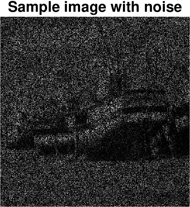
As in [20, 28], we conducted grayscale image inpainting experiments to recover low rank images from partial observations, and compare with IRcuL-q and LMaFit algorithms. The ‘boat’ image (see Figure 3) is used to produce ground truth as in [20] with rank equal to $40$ and at $512\times 512$ resolution. Different levels of noisy disturbances are added to the original image $M_{o}$ by the formula

M=M_{o}+\sigma\frac{\|M_{o}\|_{F}}{\|\varepsilon\|_{F}}\varepsilon,

where the matrix $\varepsilon$ is a standard Gaussian.

Here we only applied scheme TS1-s2. For IRucL-q, we followed the setting in [20] by choosing $\alpha=0.9$ and $\lambda=10^{-2}\sigma$ . Both fixed rank ( LMaFit-fix ) and increased rank (LMaFit-inc) schemes are implemented for LMaFit. We took fixed rank $r=40$ for TS1-s2, LMaFit-fix and IRucL-q.

Computational results are in Table IX with sampling ratios varying among $\{0.3,0.4,0.5\}$ and noise strength $\sigma$ in $\{0.01,0.05,0.10,0.15,0.20,0.25\}$ . The performance for each algorithm is measured in CPU time, PSNR (peak-signal noise ratio), and MSE (mean squared error). Here we focus more on PSNR values and placed the top $2$ in bold for each experiment. We observed that IRucL-q and TS1-s2 fared about the same. Either one is better than LMaFit in most cases.

TABLE IX: Numerical experiments on boat image inpainting with algorithms TS1, IRcuL-q and LMaFit under different sampling ratio and noise levels.

Problem		TS1-s2			IRucL-q			LMaFit-inc			LMaFit-fix
SR	$\sigma$	Time	PSNR	MSE	Time	PSNR	MSE	Time	PSNR	MSE	Time	PSNR	MSE
0.3	0.01	27.23	44.21	3.79e-5	85.97	43.28	4.70e-5	5.70	32.80	5.25e-4	2.17	45.02	3.15e-5
0.3	0.05	27.81	30.55	8.82e-4	58.25	29.55	1.11e-3	6.00	29.10	1.23e-3	2.81	29.28	1.18e-3
0.3	0.10	29.21	24.89	3.24e-3	24.26	24.99	3.17e-3	5.59	19.74	1.06e-2	5.74	18.52	1.41e-2
0.3	0.15	26.37	22.57	5.54e-3	27.61	22.74	5.33e-3	5.46	16.64	2.17e-2	4.84	15.98	2.52e-2
0.3	0.20	26.75	20.89	8.14e-3	24.45	21.05	7.85e-3	5.95	14.68	3.41e-2	3.52	14.03	3.95e-2
0.3	0.25	26.92	19.60	1.10e-2	23.75	19.75	1.06e-2	5.52	12.91	5.12e-2	1.85	12.73	5.33e-2
0.4	0.01	26.29	44.30	3.71e-5	80.19	43.25	4.74e-5	6.53	44.84	3.28e-5	2.93	45.02	3.15e-5
0.4	0.05	26.05	30.58	8.75e-4	63.20	29.39	1.15e-3	4.62	29.09	1.23e-3	3.12	27.91	1.62e-3
0.4	0.10	26.08	24.74	3.35e-3	32.58	24.86	3.27e-3	6.44	19.97	1.01e-2	8.00	19.19	1.21e-2
0.4	0.15	26.34	22.57	5.53e-3	26.30	22.72	5.35e-3	5.52	16.78	2.10e-2	2.86	16.21	2.40e-2
0.4	0.20	29.04	20.89	8.15e-3	20.73	21.08	7.81e-3	5.44	14.47	3.58e-2	2.25	14.43	3.61e-2
0.4	0.25	28.84	19.56	1.11e-2	20.48	19.68	1.08e-2	5.70	12.79	5.26e-2	2.35	12.57	5.54e-2
0.5	0.01	27.76	44.26	3.75e-5	82.42	43.30	4.67e-5	5.04	34.50	3.55e-4	2.79	45.01	3.15e-5
0.5	0.05	27.89	30.54	8.82e-4	64.19	29.47	1.13e-3	5.81	28.63	1.37e-3	2.79	29.62	1.09e-3
0.5	0.10	29.56	24.80	3.31e-3	30.50	24.94	3.21e-3	5.78	19.92	1.02e-2	3.54	19.09	1.23e-2
0.5	0.15	26.21	22.59	5.51e-3	24.24	22.74	5.32e-3	5.71	16.73	2.12e-2	2.67	16.32	2.33e-2
0.5	0.20	28.01	20.89	8.14e-3	22.51	21.07	7.82e-3	4.44	15.67	2.71e-2	2.42	14.38	3.65e-2
0.5	0.25	29.86	19.52	1.12e-2	18.32	19.71	1.07e-2	5.54	12.62	5.48e-2	3.24	12.74	5.32e-2

V Conclusion

We presented the transformed Schatten-1 penalty (TS1), and derived the closed form thresholding representation formula for global minimizers of TS1 regularized rank minimization problem. We studied two adaptive iterative TS1 schemes (TS1-s1 and TS1-s2) computationally for matrix completion in comparison with several state-of-art methods, in particular IRucL- $q$ . In case of low rank matrix recovery under known rank, TS1-s2 performs the best in accuracy and computational speed. In low rank matrix recovery under rank estimation, TS1-s1 is almost on par with IRucL-q except when both the matrix covariance and rank rise to certain level. In future work, we shall study rank estimation techniques to further improve on TS1-s1 and explore other applications for TS1 penalty.

Acknowledgments

The authors would like to thank Prof. Wotao Yin for his helpful suggestions on low rank matrix completion methods and numerical experiments.

[Proof of Ky Fan k-norm inequality]

Proof.

Since $X=U\mathrm{Diag}(\sigma)V^{T}$ , the $(j,k)$ -th entry of matrix $X$ is $X_{j,k}=\sum\limits_{i=1}^{m}\sigma_{i}U_{j,i}V_{k,i}$ .

Thus, we have

\begin{array}[]{lll}\mathrm{tr_{k}}(X)&=&\sum\limits_{j=1}^{k}X_{j,j}=\sum\limits_{j=1}^{k}\sum\limits_{i=1}^{m}\sigma_{i}U_{j,i}V_{j,i}\\ &=&\sum\limits_{i=1}^{m}\sum\limits_{j=1}^{k}\sigma_{i}U_{j,i}V_{j,i}=\sum\limits_{i=1}^{m}\sigma_{i}w_{i}^{(k)},\end{array}

(0.40)

where the weight $w_{i}^{(k)}$ for the singular value $\sigma_{i}$ is defined as:

w_{i}^{(k)}=\sum\limits_{j=1}^{k}U_{j,i}V_{j,i},\ \ i=1,2,...,m.

(0.41)

Notice that,

|w_{i}^{(k)}|\leq\sum\limits_{j=1}^{k}|U_{j,i}||V_{j,i}|\leq\|U(:,i)\|_{2}\|V(:,i)\|_{2}\leq 1,

(0.42)

where $U(:,i)$ and $V(:,i)$ are the $i$ -th column vectors for $U$ and $V$ . Also for weights $\{w_{i}^{(k)}\}$ ,

\begin{array}[]{lll}\sum\limits_{i=1}^{m}|w_{i}^{(k)}|&\leq&\sum\limits_{i=1}^{m}\sum\limits_{j=1}^{k}|U_{j,i}||V_{j,i}|=\sum\limits_{j=1}^{k}\sum\limits_{i=1}^{m}|U_{j,i}||V_{j,i}|\\ &\leq&\sum\limits_{j=1}^{k}\ \|U(j,:)\|_{2}\ \|V(j,:)\|_{2}\leq k,\end{array}

(0.43)

where $U(j,:)$ and $V(j,:)$ are the $j$ -th row vectors for $U$ and $V$ , respectively.

All the $m$ weights are bounded by $1$ , with absolute sum at most $k\leq m$ . Note that $\sigma_{i}$ ’s are in decreasing order. By equation (0.40), we have, for all $k=1,2,...,m$ ,

\mathrm{tr_{k}}(X)\leq\sum\limits_{i=1}^{m}\sigma_{i}|w_{i}^{(k)}|\leq\sum\limits_{i=1}^{k}\sigma_{i}=\mathrm{tr_{k}}(D)=\|X\|_{Fk}.

Next, we prove the second part of the lemma — equality condition, by mathematical induction. Suppose that for a given matrix $X$ , $\mathrm{tr_{k}}(X)=\mathrm{tr_{k}}(D)$ , $\forall\ k=1,...,m$ . Here, it is convenient to define $X_{i}=\sigma_{i}U_{i}V_{i}^{T}$ , where $V_{i}$ ( $U_{i}$ ) is the $i$ -th column vector of $V$ ( $U$ ). Then matrix $X$ can be decomposed as the sum of $r$ rank- $1$ matrices, $X=\sum\limits_{i=1}^{r}X_{i}$ .

When $k=1$ , according to $tr_{1}(X)=tr_{1}(D)$ and the proof above, we know that

w^{(1)}_{1}=1\ \ \text{and}\ w^{(1)}_{i}=0\ \ \text{for}\ i=2,...,m.

By the definition of weights $w_{i}^{(k)}$ in (0.41), we have $w_{1}^{(1)}=U_{1,1}V_{1,1}=1$ . Since $U$ and $V$ are both unitary matrices, we have:

U_{1,1}=V_{1,1}=\pm 1;\ \ \ U_{1,j}=U_{j,1}=V_{1,j}=V_{j,1}=0\ \text{for}\ j\neq 1.

Then vectors $U_{1}$ ( $V_{1}$ ) is the first standard basis vector in space $\Re^{m}$ ( $\Re^{n}$ ). The matrix $X_{1}=\sigma_{1}U_{1}V_{1}^{T}$ is diagonal

X_{1}=\left[\begin{array}[]{cccc}\sigma_{1}&&&\\ &0&&\\ &&\ddots&\\ &&&0\end{array}\right]_{m\times n}

For any index $i$ , $1\leq i\leq k-1$ , suppose that

U_{i,i}=V_{i,i}=\pm 1;\ \ \ U_{i,j}=U_{j,i}=V_{i,j}=V_{j,i}=0\ \text{for any index}\ j\neq i.

(0.44)

Then matrix $X_{i}=\sigma_{i}U_{i}V_{i}^{T}$ , with $1\leq i\leq k-1$ , is diagonal and can be expressed as

X_{i}=\left[\begin{array}[]{ccccccc}0&&&\\ &\ddots&&\\ &&0&\\ &&&\sigma_{i}&\\ &&&&0\\ &&&&&\ddots&\\ &&&&&&0\\ \end{array}\right]_{m\times n}\longleftarrow(i\text{-th row})

Under those conditions, let us consider the case with index $i=k$ . Clearly, we have $tr_{k}(X)=tr_{k}(D)$ . Similarly as before, thanks to the formula (0.40) and inequalities (0.42) and (0.43), it is true that

w_{i}^{(k)}=1\ \text{for}\ i=1,...,k;\ \ \ \text{and}\ w_{i}^{(k)}=0\ \text{for}\ i>k.

Furthermore, by definition (0.41), $w_{k}^{(k)}=\sum\limits_{j=1}^{k}U_{j,k}V_{j,k}=U_{k,k}V_{k,k}=1$ . This is because $U_{j,k}=V_{j,k}=0$ for index $j<k$ , by the assumption (0.44) . Thus vectors $U_{k}$ and $V_{k}$ are also standard basis vectors with the $k$ -th entry to be $\pm 1$ . Then

X_{k}=\sigma_{k}U_{k}V_{k}^{T}=\left[\begin{array}[]{ccccccc}0&&&\\ &\ddots&&\\ &&0&\\ &&&\sigma_{k}&\\ &&&&0\\ &&&&&\ddots&\\ &&&&&&0\\ \end{array}\right]_{m\times n}\longleftarrow(k\text{-th row})

Finally, we prove that all matrices $\{X_{i}\}_{i=1,\cdots,r}$ are diagonal. So the original matrix $X=\sum\limits_{i=1}^{r}X_{i}$ is equal to the diagonal matrix $D$ . The other direction is obvious. We finish the proof. ∎

References

[1] T. Blumensath, Accelerated iterative hard thresholding, Signal Processing, 92(3), pp. 752–756, 2012.
[2] J. Cai, E. J. Candès, and Z. Shen. A singular value thresholding algorithm for matrix completion. SIAM Journal on Optimization, 20(4):1956–1982, 2010.
[3] E. J. Candès and T. Tao. The power of convex relaxation: Near-optimal matrix completion. Information Theory, IEEE Transactions on, 56(5):2053–2080, 2010.
[4] E. Candès, and B. Recht, Exact matrix completion via convex optimization, Found. Comput. Math., 9 (2009), pp. 717-772.
[5] W. Cao, J. Sun, and Z. Xu, Fast image deconvolution using closed-form thresholding formulas of $L_{q},(q=1/2,2/3)$ regularization, Journal of Visual Communication and Image Representation, 24(1), pp. 31–41, 2013.
[6] Y. Chen, A. Jalali, S. Sanghavi, and C. Caramanis. Low-rank matrix recovery from errors and erasures. Information Theory, IEEE Transactions on, 59(7):4324–4337, 2013.
[7] I. Daubechies, R. DeVore, M. Fornasier, C. Gunturk, Iteratively reweighted least squares minimization for sparse recovery, Comm. Pure Applied Math, 63(1), pp. 1–38, 2010.
[8] I. Daubechies, M. Defrise, and C. De Mol. An iterative thresholding algorithm for linear inverse problems with a sparsity constraint. Communications on pure and applied mathematics, 57(11):1413-1457, 2004.
[9] D. Donoho, Denoising by soft-thresholding, IEEE Trans. Info. Theory, 41(3), pp. 613–627, 1995.
[10] P. Drineas, R. Kannan, and M. W. Mahoney. Fast monte carlo algorithms for matrices i: Approximating matrix multiplication. SIAM Journal on Computing, 36(1):132–157, 2006.
[11] P. Drineas, R. Kannan, and M. W. Mahoney. Fast monte carlo algorithms for matrices ii: Computing a low-rank approximation to a matrix. SIAM Journal on Computing, 36(1):158–183, 2006.
[12] J. Fan, and R. Li, Variable selection via nonconcave penalized likelihood and its oracle properties, Journal of the American Statistical Association, 96(456):1348–1360, 2001.
[13] K. Fan, Maximum properties and inequalities for the eigenvalues of completely continuous operators, Proc. Nat. Acad. Sci. U.S.A. 37 (1951), 760–766.
[14] M. Fazel, H. Hindi, and S. Boyd, A rank minimization heuristic with application to minimum order system approximation, In Proc. American Control Conference, Arlington, VA, 2001.
[15] M. Fazel, H. Hindi, and S. Boyd, Log-det heuristic for matrix rank minimization with applications to Hankel and Euclidean distance matrices, in Proc. Amer. Control Confer., pp. 2156–2162, Denver, CO, 2003.
[16] N. Halko, P. G. Martinsson, and J. A. Tropp. Finding structure with randomness: Probabilistic algorithms for constructing approximate matrix decompositions. SIAM review, 53(2):217–288, 2011.
[17] D. Jannach, M. Zanker, A. Felfernig, G. Friedrich, “Recommender Systems: An Introduction”, Cambridge Univ. Press, 2012.
[18] S. Ji, K-F Sze, Z. Zhou, A. So, Y. Ye, Beyond Convex Relaxation: A Polynomial-Time Non-Convex Optimization Approach to Network Localization, Proceedings of the 32nd IEEE International Conference on Computer Communications (INFOCOM 2013), 2013, pp. 2499-2507.
[19] R. Keshavan, A. Montanari, S. Oh, Matrix completion from a few entries, IEEE Trans. Info. Theory, 56 (6), 2980-2998, 2010.
[20] M. Lai, Y. Xu, and W. Yin. Improved iteratively reweighted least squares for unconstrained smoothed $l_{q}$ minimization. SIAM Journal on Numerical Analysis, 51(2):927–957, 2013.
[21] Z. Lu and Y. Zhang. Iterative reweighted singular value minimization methods for $l\_p$ regularized unconstrained matrix minimization. arXiv preprint arXiv:1401.0869, 2014.
[22] J. Lv, and Y. Fan, A unified approach to model selection and sparse recovery using regularized least squares, Annals of Statistics, 37(6A), pp. 3498–3528, September 2009.
[23] S. Ma, D. Goldfarb, and L. Chen. Fixed point and bregman iterative methods for matrix rank minimization. Mathematical Programming, 128(1-2):321–353, 2011.
[24] K. Mohan and M. Fazel. Iterative reweighted algorithms for matrix rank minimization. The Journal of Machine Learning Research, 13(1):3441–3473, 2012.
[25] F. Nie, H. Huang, and C. Ding. Low-rank matrix recovery via efficient schatten p-norm minimization. In Twenty-Sixth AAAI Conference on Artificial Intelligence, 2012.
[26] B. Recht, M. Fazel, and P. A. Parrilo. Guaranteed minimum-rank solutions of linear matrix equations via nuclear norm minimization. SIAM review, 52(3):471–501, 2010.
[27] T. Tao. Topics in random matrix theory, volume 132. American Mathematical Soc., 2012.
[28] Z. Wen, W. Yin, and Y. Zhang. Solving a low-rank factorization model for matrix completion by a nonlinear successive over-relaxation algorithm. Mathematical Programming Computation, 4(4):333–361, 2012.
[29] Z. Xu, X. Chang, F. Xu, H. Zhang, $L_{1/2}$ regularization: an iterative thresholding method, IEEE Transactions on Neural Networks and Learning Systems, 23, pp. 1013–1027, 2012.
[30] S. Zhang and J. Xin. Minimization of transformed $l\_1$ penalty: Closed form representation and iterative thresholding algorithms. to appear in Comm. Math Sciences, 2016
[31] S. Zhang and J. Xin. Minimization of transformed $l_{1}$ penalty: Theory, difference of convex function algorithm, and robust application in compressed sensing. arXiv preprint arXiv:1411.5735, 2014.
[32] Michael P Friedlander, Ives Macedo, and Ting Kei Pong. Gauge optimization and duality. SIAM Journal on Optimization, 24(4):1999–2022, 2014.
[33] Michael P Friedlander and Ives Macedo. Low-rank spectral optimization. arXiv preprint arXiv:1508.00315, 2015.
[34] Bart Vandereycken. Low-rank matrix completion by riemannian optimization. SIAM Journal on Optimization, 23(2):1214–1236, 2013.