Online Matrix Factorization via Broyden Updates
Abstract
In this paper, we propose an online algorithm to compute matrix factorizations. Proposed algorithm updates the dictionary matrix and associated coefficients using a single observation at each time. The algorithm performs low-rank updates to dictionary matrix. We derive the algorithm by defining a simple objective function to minimize whenever an observation is arrived. We extend the algorithm further for handling missing data. We also provide a mini-batch extension which enables to compute the matrix factorization on big datasets. We demonstrate the efficiency of our algorithm on a real dataset and give comparisons with well-known algorithms such as stochastic gradient matrix factorization and nonnegative matrix factorization (NMF).
Index Terms:
Matrix factorizations, Online algorithms.I Introduction
Problem of online factorization of data matrices is of special interest in many domains of signal processing and machine learning. The interest comes from either applications with streaming data or from domains where data matrices are too wide to use batch algorithms. Analysis of such datasets is needed in many popular application domains in signal processing where batch matrix factorizations is successfully applied [1]. Some of these applications include processing and restoration of images [2], source separation or denoising of musical [3, 4] and speech signals [5], and predicting user behaviour from the user ratings (collaborative filtering) [6]. Nowadays, since most applications in these domains require handling streams or large databases, there is a need for online factorization algorithms which updates factors only using a subset of observations.
Formally, matrix factorization is the problem of factorizing a data matrix into [1],
| (1) |
where and . Intuitively, is the approximation rank which is typically selected by hand. These methods can be interpreted as dictionary learning where columns of defines the elements of the dictionary, and columns of can be thought as associated coefficients. Online matrix factorization problem consists of updating and associated columns of by only observing a subset of columns of which is the problem we are interested in this work.
In recent years, many algorithms were proposed to tackle online factorization problem. In [7], authors propose an algorithm which couples the expectation-maximization with sequential Monte Carlo methods for a specific Poisson nonnegative matrix factorization (NMF) model to develop an online factorization algorithm. The model makes Markovian assumptions on the columns of , and it is similar to the classical probabilistic interpretation of NMF [8], but a dynamic one. They demonstrate the algorithm on synthetic datasets. In [9], authors propose an online algorithm to solve the Itakura-Saito NMF problem where only one column of data matrix is used in each update. They also provide a mini-batch extension to apply it in a more efficient manner and demonstrate audio applications. In [10], authors propose several algorithms for online matrix factorization using sparsity priors. In [11], authors propose an incremental nonnegative matrix factorisation algorithm based on an incremental approximation of the overall cost function with video processing applications. In [12], authors implement a stochastic gradient algorithm for matrix factorization which can be used in many different settings.
In this paper, we propose an online algorithm to compute matrix factorizations, namely the online matrix factorization via Broyden updates (OMF-B). We do not impose nonnegativity conditions although they can be imposed in several ways. At each time, we assume only observing a column of the data matrix (or a mini-batch), and perform low-rank updates to dictionary matrix . We do not assume any structure between columns of , and hence , but it is possible to extend our algorithm to include a temporal structure. OMF-B is very straightforward to implement and has a single parameter to tune aside from the approximation rank.
The rest of the paper is organised as follows. In Section II, we introduce our cost function and the motivation behind it explicitly. In Section III, we derive our algorithm and give update rules for factors. In Section IV, we provide two modifications to implement mini-batch extension and update rules for handling missing data. In Section V, we compare our algorithm with stochastic gradient matrix factorization and NMF on a real dataset. Section VI concludes this paper.
II The Objective Function
We would like to solve the approximation problem (1) by using only columns of at each iteration. For notational convenience, we denote the ’th column of with . In the same manner, we denote the ’th column of as where is the approximation rank. This notation is especially suitable for matrix factorisations when columns of the data matrix represent different instances (e.g. images). We set for .
We assume that we observe random columns of . To develop an appropriate notation, we use to denote the data vector observed at time where is sampled from uniformly random. The use of this notation implies that, at time , we can sample any of the columns of denoted by . This randomization is not required and one can use sequential observations as well by putting simply . We denote the estimates of the dictionary matrix at time as . As stated before, we would like to update dictionary matrix and a column of the matrix after observing a single column of the dataset . For this purpose, we make the following crucial observations:
- (i)
We need to ensure at time for ,
- (ii)
We need to penalize estimates in such a way that it should be “common to all observations”, rather than being overfitted to each observation.
As a result we need to design a cost function that satisfies conditions (i) and (ii) simultaneously. Therefore, for fixed , we define the following objective function which consists of two terms. Suppose we are given for and , then we solve the following optimization problem for each ,
| (2) |
where is a parameter which simply chooses how much emphasis should be put on specific terms in the cost function. Note that, Eq. (2) has an analytical solution both in and separately. The first term ensures the condition (i), that is, . The second term ensures the condition (ii) which keeps the estimate of dictionary matrix “common” to all observations. Intuitively, the second term penalizes the change of entries of matrices. In other words, we want to restrict in such a way that it is still close to after observing but also the error of the approximation is small enough. One can use a weighted Frobenius norm to define a correlated prior structure on [13], but this is left as a future work.
III Online Factorization Algorithm
For each , we solve (2) by fixing and . In other words, we will perform an alternating optimisation scheme at each step. In the following subsections, we derive the update rules explicitly.
III-A Derivation of the update rule for
To derive an update for , is assumed to be fixed. To solve for , let denote the cost function such that,
and set . We are only interested in the first term. As a result, solving for becomes a least squares problem, the solution is the following pseudoinverse operation [12],
| (3) |
for fixed .
III-B Derivation of the update rule for
If we assume is fixed, the update with respect to can be derived by setting . We leave the derivation to the appendix and give the update as,
| (4) |
and by using Sherman-Morrison formula [14] for the term , Eq. (4) can be written more explicitly as,
| (5) |
which is same as the Broyden’s rule of quasi-Newton methods as [13]. We need to do some subiterations between updates (3) and (5) for each . As it turns out, empirically, even inner iterations are enough to obtain a reliable overall approximation error.
IV Some Modifications
In this section, we provide two modifications of the Algorithm 1. The first modification is an extension to a mini-batch setting and requires no further derivation. The second modification provides the rules for handling missing data.
IV-A Mini-Batch Setting
In this subsection, we describe an extension of the Algorithm 1 to the mini-batch setting. If is too large (e.g. hundreds of millions), it is crucial to use subsets of the datasets. We use a similar notation, where instead of , now we use an index set . We denote a mini-batch dataset at time with . Hence where is the cardinality of the index set . In the same manner, denotes the corresponding columns of the . We can not use the update rule (5) immediately by replacing with (and with ) because now we can not use the Sherman-Morrison formula for (4). Instead we have to use Woodbury matrix identity [14]. However, we just give the general version (4) and leave the use of this identity as a choice of implementation. Under these conditions, the following updates can be used for mini-batch OMF-B algorithm. Update for reads as,
| (6) |
and update rule for can be given as,
| (7) |
which is no longer same as the Broyden’s rule for mini-batch observations.
IV-B Handling Missing Data
In this subsection, we give the update rules which can handle the missing data. We only give the updates for single data vector observations because deriving the mini-batch update for missing data is not obvious and also become computationally demanding as increases. So we only consider the case i.e. we assume observing only a single-column at a time.
We define a mask , and we denote the data matrix with missing entries with where denotes the Hadamard product. We need another mask to update related entries of the estimate of the dictionary matrix , which is denoted as and naturally, . Suppose we have an observation at time and some entries of the observation are missing. We denote the mask vector for this observation as which is ’th column of . We construct for each in the following way:
The use of stems from the following fact. We would like to solve the following least squares problem for (for fixed ),
| (8) |
One can easily verify that,
Then (8) can equivalently be written as,
As a result the update rule for becomes the following pseudoinverse operation,
and the update rule for (for fixed ) can trivially be given as,
We denote the results on dataset with missing entries in Experiment V-B.
V Experimental Results
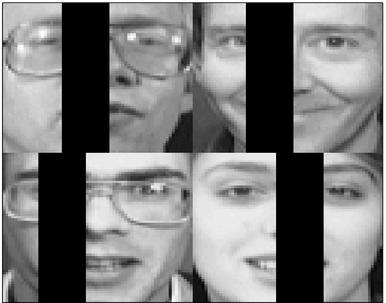
In this section, we demonstrate two experiments on the Olivetti faces dataset11 1 Available at: http://www.cs.nyu.edu/~roweis/data.html consists of faces with size of grayscale pixels. We first compare our algorithm with stochastic gradient descent matrix factorization in the sense of error vs. runtimes. In the second experiment, we randomly throw away the %25 of each face in the dataset, and try to fill-in the missing data. We also compare our results with NMF [1].
V-A Comparison with stochastic gradient MF
In this section, we compare our algorithm with the stochastic gradient descent matrix factorization (SGMF) algorithm [12]. Notice that one can write the classical matrix factorization cost as,
so it is possible to apply alternating stochastic gradient algorithm [12]. We derive and implement the following updates for SGMF,
for uniformly random for each . The following conditions hold for convergence: and and same conditions hold for . In practice we scale the step-sizes like where and . These are other parameters we have to choose for both and . It is straightforward to extend this algorithm to mini-batches [12]. We merely replace with .

In this experiment, we set identical conditions for both algorithms, where we use the Olivetti faces dataset, set , and use mini-batch size for both algorithms. We have carefully tuned and investigated step-size of the SGMF to obtain the best performance. We used scalar step sizes for the matrix and we set a step-size for each mini-batch-index, i.e. we use a matrix step-size for updating . We set . At the end, both algorithms passed times over the whole dataset taking mini-batch samples at each time. We measure the error by taking Frobenius norm of the difference between real data and the approximation.
The results are given in Fig. 1. We compared error vs. runtimes and observed that SGMF is faster than our algorithm in the sense that it completes all passes much faster than OMF-B as can be seen from Fig. 1(a). However our algorithm uses data much more efficiently and achieves much lower error rate at the same runtime by using much fewer data points than SGMF. In the long run, our algorithm achieves a lower error rate within a reasonable runtime. Additionally, our algorithm has a single parameter to tune to obtain different error rates. In contrast, we had to carefully tune the SGMF step-sizes and even decay rates of step-sizes. Compared to SGMF, our algorithm is much easier to implement and use in applications.
V-B Handling missing data on Olivetti dataset
In this experiment, we show results on the Olivetti faces dataset with missing values where %25 of the dataset is missing (we randomly throw away %25 of the faces). Although this dataset is small enough to use a standard batch matrix factorisation technique such as NMF, we demonstrate that our algorithm competes with NMF in the sense of Signal-to-Noise Ratio (SNR). We compare our algorithm with NMF in terms of number of passes over data vs. SNR. We choose , and set inner iterations as . Our algorithm achieves approximately same SNR values with NMF (1000 batch passes over data) with only 30 online passes over dataset. This shows that our algorithm needs much less low-cost passes over dataset to obtain comparable results with NMF. Numbers and visual results are given in Fig. 2.


VI Conclusions and Future Work
We proposed an online and easy-to-implement algorithm to compute matrix factorizations, and demonstrated results on the Olivetti faces dataset. We showed that our algorithm competes with the state-of-the-art algorithms in different contexts. Although we demonstrated our algorithm in a general setup by taking random subsets of the data, it can be used in a sequential manner as well, and it is well suited to streaming data applications. In the future work, we plan to develop probabilistic extensions of our algorithm using recent probabilistic interpretations of quasi-Newton algorithms, see e.g. [13] and [15]. The powerful aspect of our algorithm is that it can also be used with many different priors on columns of such as the one proposed in [16]. As a future work, we think to elaborate more complicated problem formulations for different applications.
Acknowledgements
The author is grateful to Philipp Hennig for very helpful discussions. He is also thankful to Taylan Cemgil and S. Ilker Birbil for discussions, and to Burcu Tepekule for her careful proofreading. This work is supported by the TUBITAK under the grant number 113M492 (PAVERA).
Appendix
We derive as the following. First we will find which is the derivative of the first term. Notice that
First of all the first term is not important for us, since it does not include . Using standard formulas for derivatives of traces [14], we arrive,
| (9) |
The second term of the cost function can be written as,
If we take the derivative with respect to using properties of traces [14],
| (10) |
By summing (9) and (10), setting them equal to zero, and leaving alone, one can show (4) easily. Using Sherman-Morrison formula, one can obtain the update rule given in the Eq. (5).
References
- [1] D. D. Lee and H. S. Seung, “Learning the parts of objects by non-negative matrix factorization,” Nature, vol. 401, no. 6755, pp. 788–791, Oct. 1999.
- [2] A. T. Cemgil, “Bayesian inference in non-negative matrix factorisation models,” Computational Intelligence and Neuroscience, no. Article ID 785152, 2009.
- [3] C. Fevotte, N. Bertin, and J.-L. Durrieu, “Nonnegative matrix factorization with the itakura-saito divergence: With application to music analysis,” Neural Comput., vol. 21, no. 3, pp. 793–830, Mar. 2009.
- [4] P. Smaragdis and J. C. Brown, “Non-negative matrix factorization for polyphonic music transcription,” in Applications of Signal Processing to Audio and Acoustics, 2003 IEEE Workshop on. IEEE, 2003, pp. 177–180.
- [5] K. W. Wilson, B. Raj, P. Smaragdis, and A. Divakaran, “Speech denoising using nonnegative matrix factorization with priors.” in ICASSP. Citeseer, 2008, pp. 4029–4032.
- [6] Y. Koren, R. Bell, and C. Volinsky, “Matrix factorization techniques for recommender systems,” Computer, no. 8, pp. 30–37, 2009.
- [7] S. Yildirim, A. T. Cemgil, and S. S. Singh, “An online expectation-maximisation algorithm for nonnegative matrix factorisation models,” in 16th IFAC Symposium on System Identification (SYSID 2012), 2012.
- [8] C. Fevotte and A. T. Cemgil, “Nonnegative matrix factorisations as probabilistic inference in composite models,” in Proc. 17th European Signal Processing Conference (EUSIPCO’09), 2009.
- [9] A. Lefèvre, F. Bach, and C. Févotte, “Online algorithms for nonnegative matrix factorization with the itakura-saito divergence,” in Proc. IEEE Workshop on Applications of Signal Processing to Audio and Acoustics (WASPAA), Mohonk, NY, Oct. 2011.
- [10] J. Mairal, F. Bach, J. Ponce, and G. Sapiro, “Online learning for matrix factorization and sparse coding,” The Journal of Machine Learning Research, vol. 11, pp. 19–60, 2010.
- [11] S. S. Bucak and B. Günsel, “Incremental subspace learning via non-negative matrix factorization.” Pattern Recognition, vol. 42, no. 5, pp. 788–797, 2009.
- [12] R. Gemulla, E. Nijkamp, P. J. Haas, and Y. Sismanis, “Large-scale matrix factorization with distributed stochastic gradient descent,” in Proceedings of the 17th ACM SIGKDD international conference on Knowledge discovery and data mining. ACM, 2011, pp. 69–77.
- [13] P. Hennig and M. Kiefel, “Quasi-newton methods: A new direction,” The Journal of Machine Learning Research, vol. 14, no. 1, pp. 843–865, 2013.
- [14] K. B. Petersen, M. S. Pedersen et al., “The matrix cookbook,” Technical University of Denmark, vol. 7, p. 15, 2008.
- [15] P. Hennig, “Probabilistic interpretation of linear solvers,” SIAM Journal on Optimization, vol. 25, no. 1, pp. 234–260, 2015.
- [16] N. Seichepine, S. Essid, C. Fevotte, and O. Cappe, “Piecewise constant nonnegative matrix factorization,” in Acoustics, Speech and Signal Processing (ICASSP), 2014 IEEE International Conference on. IEEE, 2014, pp. 6721–6725.