From the Kochen-Specker theorem to noncontextuality inequalities
without assuming determinism
Abstract
The Kochen-Specker theorem demonstrates that it is not possible to reproduce the predictions of quantum theory in terms of a hidden variable model where the hidden variables assign a value to every projector deterministically and noncontextually. A noncontextual value-assignment to a projector is one that does not depend on which other projectors—the context—are measured together with it. Using a generalization of the notion of noncontextuality that applies to both measurements and preparations, we propose a scheme for deriving inequalities that test whether a given set of experimental statistics is consistent with a noncontextual model. Unlike previous inequalities inspired by the Kochen-Specker theorem, we do not assume that the value-assignments are deterministic and therefore in the face of a violation of our inequality, the possibility of salvaging noncontextuality by abandoning determinism is no longer an option. Our approach is operational in the sense that it does not presume quantum theory: a violation of our inequality implies the impossibility of a noncontextual model for any operational theory that can account for the experimental observations, including any successor to quantum theory.
pacs
03.65.Ta, 03.65.UdAlthough measurements in quantum theory cannot, in general, be implemented simultaneously, one can still ask whether the outcomes of such incompatible measurements might be simultaneously well-defined within some deeper theory. To formalize this deeper theory we use the framework of ontological models [1] which generalizes the notion of a hidden variable model. Contrary to naïve impressions, it is possible to find models of this sort that reproduce quantum predictions. Problems only arise if one makes additional assumptions about the model. The Kochen-Specker theorem [2] famously derives a contradiction from an assumption we term KS-noncontextuality. Consider a set of quantum measurements, each represented by an orthonormal basis, such that some rays are common to more than one basis. It is assumed that every ontic state—a complete specification of the properties of the system, including values of hidden variables—assigns a definite value to each ray, 0 or 1, regardless of the basis (i.e. context) in which the ray appears. If a ray is assigned the value 1 (0) by an ontic state , the measurement outcome associated with that ray is predicted to occur with probability 1 (0) when any measurement including the ray is implemented on the system in ontic state . It follows that for every basis, precisely one ray must be assigned the value 1 and the others the value 0.
The assumption that the ontic state assigns a deterministic outcome to each measurement is the greatest shortcoming of the Kochen-Specker theorem. Recall that determinism is not an assumption of Bell’s theorem [3, 4]. This is evident from derivations of the Clauser-Horne-Shimony-Holt inequality [5]. Even in Bell’s original 1964 article [3], where deterministic assignments play an important role, determinism is not assumed but rather derived from local causality and the fact that quantum theory predicts perfect correlations if the same observable is measured on the two parts of a maximally entangled state (an argument from Einstein, Podolsky and Rosen [6] that Bell simply recycled [7]). It was shown in Ref. [8] that one can make a similar argument about determinism in noncontextual models: rather than assuming it, one can derive it from a generalized notion of noncontextuality and from two facts about quantum theory: (i) the outcome of a measurement of some observable is perfectly predictable whenever the preceding preparation is of an eigenstate of that observable, and (ii) the indistinguishability, relative to all quantum measurements, of different convex decompositions of the completely mixed state into pure states.
Hence, in any proof of the Kochen-Specker theorem one can replace the assumption of determinism with the generalized notion of noncontextuality and the quantum prediction of perfect predictability. If perfect predictability is indeed observed, then in the face of the resulting contradiction, one must give up on noncontextuality. This contrasts with earlier proofs where one could always salvage the generalized notion of noncontextuality by abandoning determinism.
Of course, no real experiment ever yields perfect predictability, so this manner of ruling out noncontextuality is not robust to experimental error. Following ideas introduced in recent work [9], we show how to contend with the lack of perfect predictability of measurements and derive an experimentally-robust noncontextuality inequality for any uncolourability proof of the Kochen-Specker theorem.
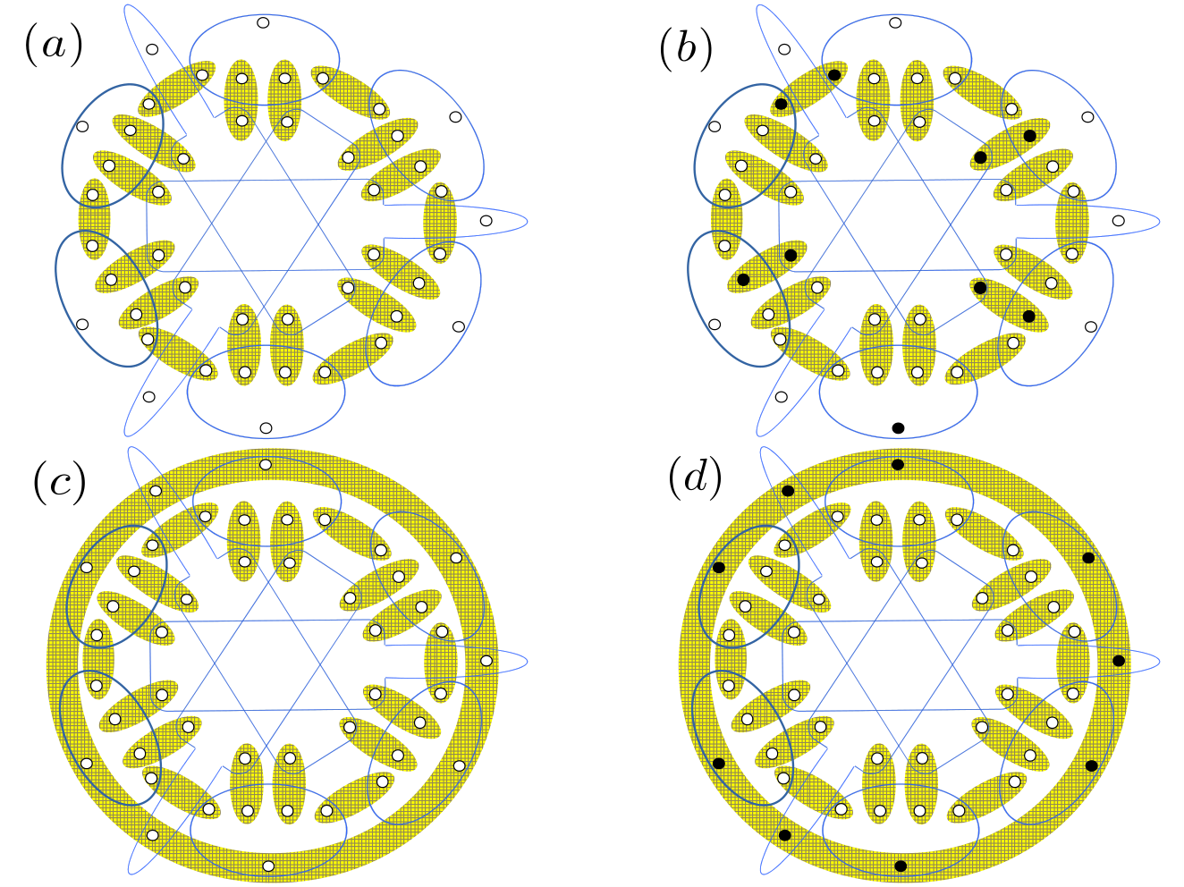
Review of the Kochen-Specker theorem. The original proof of the KS theorem required 117 rays in a 3d Hilbert space [2]. We use the much simpler proof in Ref. [10] as our illustrative example. It involves a 4d Hilbert space and 18 rays that appear in 9 orthonormal bases, each ray appearing in two bases. One can visualize this as a hypergraph with nodes representing the rays and edges representing orthonormal bases (Fig. 1(a)). There is no 0-1 assignment to these rays that respects KS-noncontextuality: the hypergraph is uncolourable (Fig. 1(b)). Of course, if the value assigned to a ray were allowed to be 0 in one basis and 1 in the other (a KS-contextual value assignment) then one could evade the contradiction.

Is it possible to test the possibility of a KS-noncontextual ontological model experimentally? One view is that the Kochen-Specker theorem is not amenable to an experimental test. It merely constrains the possibilities for interpreting the quantum formalism [11, 12]. However, this answer is clearly inadequate. One can and should ask: what is the minimal set of operational predictions of quantum theory that need to be experimentally verified in order to show that it does not admit of a noncontextual model?
We show that this minimal set is a far cry from the whole of quantum theory and is therefore consistent with many other possible operational theories. As such, the no-go result we derive shows that none of these theories admit of a noncontextual model. Furthermore, if this set of predictions is corroborated by experiment, then this implies that any future theory of physics that might replace quantum theory also fails to admit of a noncontextual model.
We begin with some definitions. An operational theory is a triple where is a set of preparations, is a set of measurements, and specifies, for every pair of preparation and measurement, the probability distribution over outcomes for that measurement if it is implemented on that preparation. Specifically, if we denote the set of outcomes of measurement by , then , is a function of the form .
An ontological model of an operational theory is a triple , where denotes a space of possible ontic states for the physical system (here presumed to be discrete), where specifies a probability distribution over the ontic states for every preparation procedure, that is, , such that , and where specifies, for every measurement, the conditional probability of obtaining a given outcome if the system is in a particular ontic state, that is, , such that . In order for the ontological model to reproduce the statistical predictions of the operational theory, it must be the case that
| (1) |
for all , and .
We denote the event of obtaining outcome of measurement by . If is assigned a deterministic outcome by every ontic state in the ontological model, i.e., if , then it is said to be outcome-deterministic in that model, and if this holds for all , then is also said to be outcome-deterministic.
We explain how to derive an experimental test of noncontextuality using a sequence of four refinements on the standard account of the KS theorem:
Operationalizing the notion of KS-noncontextuality. In a KS-noncontextual model of operational quantum theory, the value (0 or 1) assigned to the event by is the same as the value assigned to the event whenever these two events are represented by the same ray of Hilbert space (here, we are assuming that and are maximal projective measurements). We get to the crux of the notion of KS-noncontextuality, therefore, by describing the operational grounds for associating the same ray to as is associated to . Letting and represent the corresponding rank-1 projectors, the grounds for concluding that are that for an appropriate set of density operators . It is clearly sufficient for the equality to hold for the set of all density operators, but it is also sufficient to have equality for certain smaller sets of density operators, namely, those complete for measurement tomography, or simply tomographically complete.
What then should the operational grounds be for assigning the same value to and in a general operational theory, where preparations are not represented by density operators? The answer, clearly, is that the event occurs with the same probability as the event for all preparation procedures of the system,
| (2) |
or equivalently, if this holds for a subset of that is tomographically complete. In this case, we shall say that and are operationally equivalent, and denote this as . We can therefore define a notion of KS-noncontextuality for any operational theory as follows: an ontological model of an operational theory is KS-noncontextual if (i) operational equivalence of events implies equivalent representations in the model, i.e., for all , and (ii) the model is outcome-deterministic,
The operational equivalences among the measurements that are relevant for the 18 ray proof of the KS theorem depicted in Fig. 1(a) are made explicit in Fig. 2(a), where every measurement event is represented by a distinct node, and a novel type of edge between nodes specifies when two events are operationally equivalent. This representation affords a nice way of depicting contextual value assignments, such as in Fig. 2(b). It follows that any operational theory that admits of nine four-outcome measurements that satisfy the operational equivalence relations depicted in Fig. 2(a) fails to admit of a KS-noncontextual model.

Defining a notion of noncontextuality without outcome determinism. The essence of noncontextuality is that context-independence at the operational level should imply context-independence at the ontological level. The operationalized version of KS-noncontextuality commits one to more than this, however, because it makes an additional assumption about what sort of thing should be independent of context at the ontological level, namely, a deterministic assignment of an outcome. However, one can equally well assume that the ontic state merely assigns a probability distribution over outcomes, and take this distribution to be the thing independent of the context. In Ref. [8], this revised notion of noncontextuality was termed measurement noncontextuality:
Measurement noncontextuality is satisfied by an ontological model of an operational theory if implies for all .
Here, (and not merely ). Outcome determinism is not assumed.
Justifying outcome determinism for perfectly predictable measurements. Outcome determinism can, however, be justified sometimes if one assumes a notion of noncontextuality for preparations [8]. First, a definition: and are said to be operationally equivalent, denoted , if for every measurement event , assigns the same probability to this event as does, that is,
| (3) |
A preparation-noncontextual ontological model is then defined as follows:
Preparation noncontextuality is satisfied by an ontological model of an operational theory if implies for all .
Insofar as both measurement and preparation noncontextuality are instances of operational equivalence implying ontological equivalence, it is most natural to assume both, that is, to assume universal noncontextuality.
It was shown in Ref. [8] that in a preparation-noncontextual model of quantum theory, all projective measurements must be represented outcome-deterministically. Here, we provide a version of this argument for the 18 ray construction.
Suppose that one has experimentally identified thirty-six preparation procedures organized into nine ensembles of four each, , such that for all , measurement on preparation yields the th outcome with certainty,
| (4) |
We call this property perfect correlation. In quantum theory, it suffices to let be the preparation associated with the pure state corresponding to the th element of the th measurement basis.

Define the effective preparation as the procedure obtained by sampling uniformly at random and then implementing . We now suppose that one has experimentally verified the operational equivalence relations
| (5) |
These equivalences are depicted in Fig. 3. They hold in our quantum example because the simply correspond to different ways of preparing the completely mixed state.
Given Eq. (5) and the assumption of preparation noncontextuality, there is a single distribution over , denoted , such that
| (6) |
Given the definition of , it follows that
| (7) |
Because every in the support of appears in the support of for some , it follows that if had an indeterministic response on any such , we would have a contradiction with Eq. (8). Consequently, for all and , the measurement event must be outcome-deterministic for all in the support of .
To summarize then, if one has experimentally verified the operational equivalences depicted in Figs. 2(a) and 3 and the measurement statistics described in Eq. (4), then universal noncontextuality implies that the value assignments to measurement events should be deterministic and noncontextual, hence KS-noncontextual, and we obtain a contradiction in the usual manner. The argument can be summarized thus
| (9) |
Contending with the lack of perfect predictability in real experiments. In real experiments, the ideal of perfect correlation described by Eq. (4) is never achieved, so we cannot derive a contradiction from it. However, Eq. (9) is logically equivalent to the following inference:
| (10) |
This means that the amount of correlation, averaged over all and , will necessarily be bounded away from 1. It is this bound that is the operational noncontextuality inequality. For the 18 ray example, we prove that
| (11) |
To test the assumption of noncontextuality, therefore, one must measure the correlation for all and , but one must also verify that the operational equivalences depicted in Figs. 2(a) and 3 hold, because only in this case does the assumption of noncontextuality imply that the inequality (11) should hold.
We now outline how the bound in Eq. (11) is obtained. First, we use Eq. (1) to express in terms of and . Defining the max-predictability of a measurement given an ontic state by
| (12) |
The measurements can have indeterministic responses, , but measurement noncontextuality implies that for the operationally equivalent pairs . There are many such assignments. Every unit-trace positive operator, for instance, specifies an indeterministic noncontextual assignment via the Born rule, and there are other, nonquantum assignments as well, such as the one depicted in Fig. 4.

Consider the average max-predictability achieved by the assignment of Fig 4. Here, six measurements have max-predictability 1, while three have max-predictability . This implies that . As we demonstrate in Appendix A, no ontic state has a higher average max-predictability than that of Fig. 4, so that , thereby establishing the noncontextual bound on . The logical limit for the value of is , so the noncontextual bound of is nontrivial. The quantum realization of the 18 ray construction achieves .
Note that if an experiment fails to suppress noise sufficiently, then it may not succeed in violating our noncontextuality inequality. This simple criterion of operational meaningfulness fails for previous attempts at deriving noncontextuality inequalities [13], a point we discuss further in Appendices B and C. Although we have used the 18 ray uncolourable set of Ref. [10] as an example, the scheme described can be used to turn any proof of the Kochen-Specker theorem based on an uncolourable set into an experimental inequality. An issue we haven’t addressed is that in practice no two measurement events are assigned exactly the same probability by each of a tomographically complete set of preparations, nor do any two preparations assign exactly the same probability distribution over outcomes to each of a tomographically complete set of measurements. The solution to this problem is described in related work [9, 14]. A question that remains is: how does one accumulate evidence that a given set of measurements or preparations is indeed tomographically complete? This question represents the new frontier in the project of devising strict experimental tests of the assumption of noncontextuality.
Acknowledgments: RK thanks the Perimeter Institute and the Institute of Mathematical Sciences for supporting his visit during the course of this work. This project was made possible in part through the support of a grant from the John Templeton Foundation. Research at Perimeter Institute is supported by the Government of Canada through Industry Canada and by the Province of Ontario through the Ministry of Economic Development and Innovation.
References
- [1] The ontological models framework has the advantage of not prejudicing the question of whether any of the variables remain unkown (i.e. hidden) to one who knows the preparation procedure. For an overview, see N. Harrigan and R. W. Spekkens, Einstein, Incompleteness, and the Epistemic View of Quantum States, Found. Phys. 40, 125 (2010).
- [2] S. Kochen and E. P. Specker, The Problem of Hidden Variables in Quantum Mechanics, J. Math. Mech. 17, 59 (1967).
- [3] J. S. Bell, On the Einstein-Podolsky-Rosen Paradox, Physics 1, 195 (1964). Reprinted in Ref. [22], chap. 2.
- [4] J. S. Bell, On the problem of hidden variables in quantum mechanics, Rev. Mod. Phys. 38, 447 (1966); Reprinted in Ref. [22], chap. 1.
- [5] J. F. Clauser, M. A. Horne, A. Shimony, and R. A. Holt, Proposed Experiment to Test Local Hidden-Variable Theories, Phys. Rev. Lett. 23, 880 (1969).
- [6] A. Einstein, B. Podolsky, and N. Rosen, Can Quantum-Mechanical Description of Physical Reality Be Considered Complete?, Phys. Rev. 47, 777 (1935).
- [7]
Indeed, in Ref. [22] (p. 157), Bell writes
Although Wiseman has disputed Bell’s account of the role of determinism in his first paper[19], see Norsen’s response[20].My own first paper on [the subject of Bell’s Theorem] … starts with a summary of the EPR argument from locality to deterministic hidden variables. But the commentators have almost universally reported that it begins with deterministic hidden variables.
- [8] R. W. Spekkens, Contextuality for preparations, transformations, and unsharp measurements, Phys. Rev. A 71, 052108 (2005).
- [9] M. D. Mazurek, M. F. Pusey, R. Kunjwal, K. J. Resch, and R. W. Spekkens, An experimental test of noncontextuality without unwarranted idealizations, arXiv:1505.06244 (quant-ph) (2015).
- [10] A. Cabello, J. Estebaranz, and G. Garcia-Alcaine, Bell-Kochen-Specker theorem: A proof with 18 vectors, Physics Letters A 212, 183 (1996).
- [11] D. A. Meyer, Finite Precision Measurement Nullifies the Kochen-Specker Theorem, Phys. Rev. Lett. 83, 3751 (1999); A. Kent, Noncontextual Hidden Variables and Physical Measurements, Phys. Rev. Lett. 83, 3755 (1999); R. Clifton and A. Kent, Simulating quantum mechanics by non-contextual hidden variables, Proc. R. Soc. Lond. A: 2000 456 2101-2114 (2000); J. Barrett and A. Kent, Non-contextuality, finite precision measurement and the Kochen-Specker theorem, Stud. Hist. Philos. Mod. Phys. 35, 151 (2004).
- [12] Indeed, in Ref. [21], David Mermin is quoted as having said: “the whole notion of an experimental test of [B]KS misses the point”, a view that was held by many researchers at the time.
- [13] A. Cabello, Experimentally testable state-independent quantum contextuality, Phys. Rev. Lett. 101, 210401 (2008).
- [14] M. F. Pusey, The robust noncontextuality inequalities in the simplest scenario (2015).
- [15] R. W. Spekkens, Negativity and Contextuality are Equivalent Notions of Nonclassicality, Phys. Rev. Lett. 101, 020401 (2008).
- [16] A. Cabello, S. Severini, and A. Winter, Graph-Theoretic Approach to Quantum Correlations, Phys. Rev. Lett. 112, 040401 (2014).
- [17] A. Acin, T. Fritz, A. Leverrier, and A. B. Sainz, A Combinatorial Approach to Nonlocality and Contextuality, Comm. Math. Phys. 334(2), 533-628 (2015).
- [18] R. W. Spekkens, The Status of Determinism in Proofs of the Impossibility of a Noncontextual Model of Quantum Theory, Found. Phys. 44, 1125 (2014).
- [19] H. M. Wiseman, The Two Bell’s theorems of John Bell, J. Phys. A: Math. Theor. 47 424001 (2014).
- [20] T. Norsen, Are there really two different Bell’s theorems, arXiv:1503.05017 (quant-ph) (2015).
- [21] A. Cabello and G. Garcia-Alcaine, Proposed Experimental Tests of the Bell-Kochen-Specker Theorem, Phys. Rev. Lett. 80, 1797 (1998).
- [22] J. S. Bell, Speakable and unspeakable in quantum mechanics (Cambridge University Press, New York, 1987).
Appendix A Proof of the inequality
We can summarize our main result—a derivation of a noncontextuality inequality from the proof of the Kochen-Specker theorem for the 18 ray uncolourable set of Fig. 1—by the following theorem:
Theorem.
Consider an operational theory . Let be nine four-outcome measurements. Let denote the th outcome of the th measurement, where . Let , be thirty-six preparation procedures, organized into nine sets of four. Let be the preparation procedure obtained by sampling uniformly at random and implementing .
Suppose that one has experimentally verified the operational preparation equivalences depicted in Fig. 3, namely,
| (14) |
and the operational equivalences depicted in Fig. 2(a), namely,
| (15) |
for the eighteen pairs specifed therein.
If one assumes that the operational theory admits of a universally noncontextual ontological model, that is, one which is both measurement-noncontextual and preparation-noncontextual, then the following inequality on operational probabilities holds
| (16) |
We now provide the proof. For clarity, we expand on some of the steps presented in the main article.
Using Eq. (1), the quantity can be expressed in terms of the distributions and response functions of the ontological model as
| (17) |
Using the definition of the max-probability , given in Eq. (12), we have
| (18) |
Assuming that one experimentally verifies the operational preparation equivalences of Eq. (14), the assumption of preparation noncontextuality implies that
| (19) |
It follows that there exists a single distribution, which we denote , such that
| (20) |
Recall that is the preparation procedure that samples uniformly from and implements . Given that the probability of the system being in a given ontic state given the preparation is , and given that the probability of being implemented is for each value of , it follows that the probability of the system being in a given ontic state given the preparation is . Combining this with Eq. (20), we conclude that
| (21) |
and therefore that
| (22) |
This in turn implies
| (23) |
Assuming that one experimentally verifies the operational measurement equivalences of Eq. (15), the assumption of measurement noncontextuality implies that
| (24) |
for the eighteen pairs of operationally equivalent measurement events specifed in Fig. 2(a).
It is useful to simplify the notation at this stage. We introduce the variable to range over the eighteen operational equivalence classes of measurement events. We introduce the shorthand notation
| (25) |
for the probability assigned to the th equivalence class, where the dependence on is left implicit. The variable enumerates the equivalence classes in Fig. 2(a) starting from and proceeding clockwise around the hypergraph, as depicted in Fig. 5.

In this notation, the constraint that each response function is probability-valued, , is simply
| (26) |
while the constraint that the set of response functions for each measurement sum to 1, , can be captured by the matrix equality
| (27) |
where , , and
| (28) |
Finally, we can express the quantity to be maximized as
| (29) |
or, more explicitly, as
| (30) |
The matrix equality of Eq. (27) implies that there are only nine independent variables in the set and that these satisfy linear inequalities. The space of possibilities for the vector therefore forms a nine-dimensional polytope in the hypercube described by Eq. (26).
The value of on any of the interior points of this polytope will be an average of its values at the vertices because it is a convex function of . Therefore, to implement the maximization over , it suffices to maximize over the vertices of this polytope.
Following a brute-force enumeration of all the vertices of the polytope, the maximum possible value of is found to be . An example of a vertex achieving this value is , which is depicted in Fig. 4. This concludes the proof.
Our proof technique can be adapted to derive a similar noncontextuality inequality correponding to any proof of the KS theorem based on the uncolourability of a set of rays of Hilbert space. One begins by completing every set of orthogonal rays into a basis of the Hilbert space, and then forming the hypergraph depicting the orthogonality relations among these rays (the analogue of Fig. 1). One then forms the hypergraph decipting all of the measurements events, with one type of edge denoting which events correspond to the outcomes of a single measurement, and the other type of edge denoting when a set of measurement events are operationally equivalent (the analogue of Fig. 2(a)). One then associates a set of preparations with every measurement in the hypergraph, one preparation for every outcome. For each such set of preparations, we define the effective preparation that is the uniform mixture of the set’s elements, and we presume that all of the effective preparations so defined are operationally equivalent (as is the case in quantum theory, where the effective preparation for every set corresponds to the completely mixed state). We consider the correlation between the measurement outcome and the choice of preparation in the set associated with that measurement, averaged over all measurements. This average correlation is the quantity that appears on the left-hand side of the operational inequality.
The uncolourability of the hypergraph means that there are no noncontextual deterministic assignments to the measurement events, hence the polytope of probabilistic assignments to the measurement events has no deterministic vertices either. Each vertex of this polytope, that is, each convexly-extremal probabilistic assignment, will necessarily yield an indeterministic assignment to some of the measurement events. Using the operational equivalences and the assumption of universal noncontextuality, one can infer from this that the average correlation is always bounded away from 1. For any uncolourable hypergraph, a quantum realization would achieve the logical limit by construction, so the noncontextuality inequality we derive is necessarily violated by quantum theory in each case.
One can understand this violation as being due to the fact that assignments of density operators that are independent of the preparation context can achieve higher predictability for the respective measurements than assignments of probability distributions over ontic states that are independent of the preparation context. This is the feature of quantum theory that allows it to maximally violate the noncontextual bound of .
Appendix B Robustness of the noncontextuality inequality to noise
How much noise can one add to the measurements and preparations while still violating our noncontextuality inequality? We answer this question here assuming that the experimental operations are well-modelled by quantum theory. According to quantum theory,
| (31) |
where denotes the positive operator representing the measurement event and denotes the density operator representing the preparation . To be precise, for every , the set is a positive operator valued measure, so that , and , and for every and , is positive, , and has unit trace, .
In quantum theory, a noiseless and maximally informative measurement is represented by a POVM whose elements are rank-1 projectors, that is,
| (32) |
where for each , is a projector, hence idempotent, , and is rank , so that , where for each , the set is an orthonormal basis of the Hilbert space. If we furthermore set
| (33) |
then we find for each , and consequently . We see, therefore, that the maximum possible value of is attained when measurements satisfy the noiseless ideal. We can now consider the consequence of adding noise.
We begin by considering a very simple noise model wherein the preparations and measurements both deviate from the noiseless ideal by the action of a depolarizing channel, that is, a channel of the form
| (34) |
which with probability implements the identity channel and with probability generates the completely mixed state. If the quantum states are the image of the ideal states under a depolarizing channel with parameter , and the POVM is obtained by acting the depolarizing channel with parameter followed by the ideal projector-valued measure (such that the POVM elements are the images of the projectors under the adjoint of the channel), then
| (35) | |||||
| (36) |
Here, the POVM is a mixture of and a POVM which simply samples uniformly at random regardless of the input state. It follows that for each , if we consider , we find perfect predictability for the term having weight while for the three other terms, we have a uniformly random outcome, so that in all
| (37) |
It follows that
| (38) |
Thus a violation of the noncontextuality inequality, i.e. , occurs if and only if
| (39) |
It turns out that one can derive similar bounds for more general noise models as well. Suppose that instead of a depolarizing channel, we have one of the form
| (40) |
With probability , this implements the identity channel and with probability it reprepares a state that need not be the completely mixed state, but which is independent of the input to the channel. The analogous sort of noise acting on the measurement corresponds to acting on the POVM elements by the adjoint of this channel, that is,
| (41) |
Therefore, if this sort of noise is applied to the ideal states and measurements, with the parameters in each noise model allowed to depend on , we obtain
| (42) | |||||
where is a probability distribution over for each value of . Here, the POVM is a mixture of and a POVM which simply samples at random from the distribution , regardless of the quantum state. Compared to the simple model considered above, the innovation of this one is that for both preparations and measurements, the noise is allowed to be biased.
For the case of , which by Eq. (42) implies that , we find that, regardless of the measurement, is just a normalized probability distribution over (because there is no dependence in the state). Hence, in this case, .
Similarly, for the case of , that is, when the POVM corresponds to a random number generator , we find that, regardless of the preparation, is again just a normalized probability distribution over . Hence, in this case again, .
It follows that for generic values of and , we have . In all then, we have
| (44) |
Consequently, a violation of the noncontextuality inequality, i.e., , occurs if and only if the noise parameters satisfy
| (45) |
Because the parameters and decrease as one increases the amount of noise, this inequality specifies an upper bound on the amount of noise that can be tolerated if one seeks to violate the noncontextuality inequality.
This analysis highlights how the approach to deriving noncontextuality inequalities described in this article has no trouble accommodating noisy POVMs. This contrasts with previous proposals for experimental tests based on the traditional notion of noncontextuality, which can only be applied to projective measurements. This is one way to see how previous proposals are not applicable to realistic experiments, where every measurement has some noise and consequently is necessarily not represented projectively.
Appendix C Comparison to other noncontextuality inequalities
We have proposed a technique for deriving noncontextuality inequalities from proofs of the Kochen-Specker theorem. It is useful to compare our approach with one that has previously been proposed by Cabello [13]. We do so by explicitly comparing the two proposals in the case of the 18 ray construction of Ref. [10]. Indeed, the fact that Ref. [13] proposes an inequality for this construction is part of our motivation for choosing it as our illustrative example.
For each of the eighteen operational equivalence classes of measurement events, labelled by as depicted in Fig. 5, we associate a -valued variable, denoted . A given ontic state is assumed to assign a value to each . The fact that there is only a single variable associated to each equivalence class implies that any assignment of such values is necessarily noncontextual.
Ref. [13] considers a particular linear combination of expectation values of products of these variables:
| (46) |
and derives the following inequality for it:
| (47) |
(Note that Ref. [13] used a labelling convention for the eighteen measurement events that is different from the one we use here; to translate between the two conventions, it suffices to compare Fig. 1 in that article with Fig. 5 in ours.) Each term in refers to a quadruple of variables that can be measured together, that is, which can be computed from the outcome of a single measurement. Different terms correspond to measurements that are incompatible.
In Ref. [13], the following justification is given for the inequality (47). We are asked to consider the possible assignments to that result from the two possible assignments to , namely or , for each . It is then noted that among all such possibilities, the maximum value of that can be achieved is 7.
Ref. [13] states that a violation of this inequality should be considered evidence of a failure of noncontextuality. We disagree with this conclusion, and the rest of this section seeks to explain why.
C.1 The most natural interpretation
It is useful to recast the inequality of Eq. (47) in terms of variables with values in rather than . Specifically, we take
| (48) |
Under this translation, products of the correspond to sums (modulo 2) of the . For instance, an equation such as corresponds to the equation , where denotes sum modulo 2, while corresponds to , so that . In particular, we also have
| (49) |
or equivalently,
| (50) |
We can therefore consider a quantity , defined as
| (51) |
so that , and we can re-express inequality (47) as
| (52) |
Of course, rather than using Eq. (50) to translate (47) from -valued variables into -valued variables, one can also just derive the inequality (52) directly: among the possible assignments of values in to each of the , the maximum value of is 8. Two examples of such assignments are provided in Fig. 6.

It is useful to use a notation that specfies whether a given expectation value of some variable is relative to a preparation procedure , in which case it is denoted , or relative to an ontic state , in which case it is denoted . We denote by the quantity defined in (51) if the expectation values contained therein are relative to preparation , and we denote by the case where the expectation values are relative to ontic state . Under the assumption of an ontological model, each expectation value relative to a preparation can be expressed as a function of the expectation value relative to an ontic state , via
| (53) |
where is the distribution over ontic states associated with preparation . We can infer from Eq. (53) that
| (54) |
With these notational conventions, we can summarize the argument of Ref. [13] as follows. In any noncontextual ontological model, every ontic state satisfies
| (55) |
But this in turn implies, through Eq. (54), that for all preparations ,
| (56) |
which is an inequality constraining operational quantities.
We are now in a position to describe the problem with the inequality (56), or equivalently inequality (47), and thus with the claim of Ref. [13]. First, we highlight the physical interpretation of the variables . If is assigned value 1 by the ontic state , then this means that if the system is in the ontic state , and a measurement that includes as an outcome is implemented on it, then the outcome is certain to occur, while if is assigned value 0 by , then the outcome is certain not to occur. But each of the different assignments to is such that for at least one measurement either: none of the outcomes occur, as in the example of Fig. 6(a), or more than one outcome occurs, as in the example of Fig. 6(b). (This is precisely what is implied by the fact that the 18 measurement events are uncolourable, as explained in the main text.) Such assignments involve a logical contradiction given that the four outcomes of each measurement are mutually excusive and jointly exhaustive possibilities.
It follows that the sort of model that a violation of inequality (56) rules out can already be ruled out by logic alone; no experiment is required. To put it another way, discovering that quantum theory and nature violate inequality (56) only allows one to conclude that neither quantum theory nor nature involve a logical contradiction, which one presumably already knew prior to noting the violation.
We have argued in the main text that the notion of KS-noncontextuality, insofar as it assumes outcome-determinism, is not suitable for devising experimentally robust inequalities given that every real measurement involves some noise. The problem with inequality (56) can also be traced back to the use of the assumption of KS-noncontextuality. Suppose we ask the following question: given the existence of nine four-outcome measurements satisfying the operational equivalences of Fig. 2(a), how are the operational probabilities that are assigned to these measurement events constrained if we presume that KS-noncontextual assignments underlie the operational statistics? On the face of it, the question seems well-posed. On further reflection, however, one sees that it is not. There are simply no KS-noncontextual assignments to these measurement events, so it is simply impossible to imagine that such assignments could underlie the operational statistics. There is nothing to be tested experimentally, as the hypothesis under consideration is seen to be false as a matter of logic.
Here is another way to see that the inequality (56) does not provide a test of noncontextuality. Consider the expectation value for a preparation , where , , and correspond to the four outcomes of some measurement. Regardless of which of the four outcomes of the measurement occurs in a given run where preparation is implemented—i.e. regardless of whether comes out as (1,0,0,0) or (0,1,0,0) or (0,0,1,0) or (0,0,0,1) in that run—the variable has the value 1. We can think of it this way: the variable is a trivial variable because it is a constant function of the measurement outcome. (This is analogous to how, in quantum theory, for a four-outcome measurement associated with four projectors, although each projector is a nontrivial observable, their sum is the identity operator, which has expectation value 1 for all quantum states, and therefore corresponds to a trivial observable.) It follows that regardless of what distribution over the four outcomes is assigned by , the expectation value will be 1. Given that each of the nine terms in is of this form, it follows that .
So, for any operational theory that admits of nine four-outcome measurements with the operational equivalence relations depicted in Fig. 2(a), we will find that for all . Therefore, we can conclude that the inequality is violated for all . One can reach this conclusion without ever considering the question of whether the operational predictions can be explained by some underlying noncontextual model.
Another consequence of the triviality of the variables of the form is that the inequality (56) can be violated regardless of how noisy the measurements are. Suppose, for instance, that quantum theory describes our experiment, but that the nine four-outcome measurements are not the projective measurements described in Fig. (1), but rather noisy versions thereof. For instance, one can imagine that each measurement is associated with a positive operator-valued measure that is the image under a depolarizing map of the projector valued measure associated with the ideal measurement. The amount of depolarization can be taken arbitrarily large and, as long as it is the same amount of depolarization for each of the measurements, the nine noisy measurements that result will still satisfy precisely the same operational equivalences as the original nine, namely, those depicted in Fig. 2(a). For such noisy measurements, we can still identify variables associated to the eighteen equivalence classes of measurement events, and we still find that regardless of which of the four outcomes of the measurement occurs, the variable has the value 1, so that regardless of what distribution over the four outcomes is assigned by , the expectation value will be 1 and therefore , which is a violation of the inequality (56).
According to the generalized notion of noncontextuality proposed in Ref. [8], if one adds enough noise to the preparations and measurements in an experiment, it always becomes possible to represent the experimental statistics by a noncontextual model. One way to prove this is to note that: (i) if all of the preparations and the measurements in an experiment admit of positive Wigner representations, then, as demonstrated in Ref. [15], the Wigner representation defines a noncontextual model, and (ii) if one adds enough noise to the preparations and measurements, it is possible to ensure that they admit of positive Wigner representations.
This analysis of the effect of noise accords with intuition: noncontextuality is meant to represent a notion of classicality, so that a failure of noncontextuality is only expected to occur in a quantum experiment if one’s experimental operations have a high degree of coherence. It follows that there should always exist a threshold of noise above which an experiment cannot be used to demonstrate the failure of noncontextuality. One can turn this observation into a minimal criterion that should be satisfied by any noncontextuality inequality: there should exist a threshold of experimental noise above which a noncontextuality inequality cannot be violated.
As we have just noted, the inequality proposed in Ref. [13] fails this minimal criterion. By contrast, the noncontextuality inequality proposed in this article identifies such a threshold for the 18 ray construction: the noise must be kept low enough that the average of the measurement predictabilities is above .
C.2 Alternative interpretation
The inequality proposed in Ref. [13] can be given a different interpretation to the one provided in the previous subsection. This interpretation is more charitable in some ways, but it still does not vindicate the proposed inequality as delimiting the boundary of noncontextual models.
The idea is to imagine that for each of the nine measurements, there are in fact five rather than four outcomes that are mutually exclusive and jointly exhaustive. Thus, in this interpretation, it is assumed that the hypergraph describing compatibility relations and operational equivalences is not the one of Fig. 2(a), but rather a modification wherein there are nine additional nodes—one additional node appended to each of the nine measurements—as depicted in Fig. 7(a).
If are the original four outcomes of a given measurement, then the variable is no longer a constant function of the measurement outcome because its value varies depending on whether or not the fifth outcome occurs. If denotes the fifth outcome of the measurement, then the trivial variable is , taking the value 1 regardless of the outcome.
In this case, the assignments of the type depicted in Fig. 6(a)—the noncontextual deterministic assignments that are subnormalized—can be embedded into noncontextual deterministic normalized assignments on the larger hypergraph, as depicted in Fig. 7(b). (The possibility of such an embedding for the subnormalized noncontextual deterministic assignments considered in Cabello, Severini and Winter [16] was noted in Acin, Fritz, Leverrier, Sainz [17].)
Of course, such a move does not provide any way of understanding the deterministic noncontextual assignments of the type depicted in Fig. 6(b), because the latter violate normalization by having the probabilities of the different outcomes of the measurement summing to greater than 1—they are supernormalized.
So, while the supernormalized noncontextual deterministic assignments can be ruled out by logic alone, the subnormalized noncontextual deterministic assignments may be entertained without logical inconsistency if they are considered as reductions to a subgraph of a normalized noncontextual deterministic assignment on a larger hypergraph.
Because the justification given in Ref. [13] for the inequality derived there asks one to consider all of the noncontextual deterministic assignments, including the supernormalized ones, the interpretation of this inequality as a constraint on subnormalized assignments is in tension with the manner in which the inequality is justified. This interpretation is a better fit with Cabello’s later work, such as Ref. [16], wherein the restriction to subnormalized assignments is explicit. In any case, if the inequality holds for all noncontextual deterministic assignments, regardless of normalization, then it holds for the special case of the subnormalized assignments, so the inequality can still be derived within this interpretation.
The problem with this interpretation becomes manifest when we require that the original hypergraph of Fig. 2(a)—and thus the corresponding subgraph of Fig. 7(a) from which it is derived in this interpretation—is realized in terms of Hilbert-space bases in the manner depicted in Fig. 1(a).
We consider two possible ways of fulfiling this requirement, and explain why it is not possible to vindicate the inequality of Eq. (52) in either case.
In one approach, we imagine that the quantum system is in fact described by a 5-dimensional Hilbert space. In this case, rank-1 projective measurements have five outcomes and are therefore described within the hypergraph representation by an edge with five nodes, just as we have for the measurements in Fig. 7(a). Now consider an association of Hilbert space rays with the nodes of this hypergraph such that one recovers the association of rays to nodes described by Fig. 1 on the subgraph of Fig. 7(a) that corresponds to the original hypergraph of Fig. 2(a). This is possible if, for every measurement, the fifth outcome is associated with a ray that is orthogonal to the 4d subspace in which all of the other rays live. But then, under a tomographically complete set of preparations of the 5d Hilbert space, one finds that the fifth outcomes are all operationally equivalent, so that the appropriate hypergraph is not that of Fig. 7(a) but rather the one depicted in Fig. 7(c).
Now, consider this hypergraph. It only admits of a single normalized noncontextual deterministic assignment, the one that assigns 0s to every outcome in the original set and 1 to all of the fifth outcomes, as depicted in Fig. 7(d). Therefore, if one were to experimentally verify the applicability of the hypergraph of Fig. 7(c), by verifying the operational equivalences depicted therein, then any KS-noncontextual model consistent with this hypergraph would not only satisfy the inequality (Eq. (55)), it would predict that all of the measurement events appearing in the inequality receive value 0, so that the inequality could be strengthened to the equality , which in turn would imply, through Eq. (54), that for all preparation procedures , the operational inequality could be strengthened to the operational equality
| (57) |
But this is trivial to violate experimentally: simply find a preparation that does not always yield the fifth outcome for every measurement.
We take the triviality of this constraint to speak against the idea that it captures the assumption of noncontextuality. Therefore, the conclusion to draw from this discussion is not that one should replace the inequality with . Rather, as we’ve argued at length in the main text, because the KS-noncontextual models make the unjustified assumption of outcome-determinism, the notion of noncontextuality should not be formalized as KS-noncontextuality, but rather as measurement and preparation noncontextuality.
We now turn to the second approach. Here, one sticks to the notion that the quantum system being probed is 4-dimensional and instead one suggests that each of the nine measurements is nonprojective, that is, each is represented by a positive operator valued measure rather than a projector valued measure. In this way, one can ensure that the measurements indeed have five outcomes. One might even think of the fifth outcome as representing a ‘no detection’ event (the idea of justifying subnormalized assignments by imagining an additional ‘no detection’ outcome has also been discussed in Ref. [17]).
To see that there is something fishy about this approach, it suffices to note that if it were correct, then it would have the bizarre consequence that in the case where the measurements achieve the ideal of projectiveness, satisfaction of the inequality is ruled out by logic alone, whereas if the measurements depart from this ideal, however little, suddenly the inequality specifies whether or not the experiment can be modelled noncontextually.
In any case, the real problem with this approach is easily identified. For a nonprojective measurement, one is assigning probabilities to effects (positive operators less than identity) rather than projectors. In this case, one must allow noncontextual assignments to be probabilistic. This has been proven elsewhere [18] and we will not repeat the arguments here. Such probabilistic noncontextual assignments are not restricted to be in the convex hull of the deterministic noncontextual assignments, and therefore can be more general than mixtures of the latter. Because the derivation of the inequality made crucial use of the assumption that the preparation was a mixture of deterministic noncontextual assignments, the fact that the assumption of determinism is unwarranted implies that one can no longer derive the inequality as a constraint on noncontextual models.