Generation of large-scale magnetic fields by small-scale dynamo in shear flows
Abstract
We propose a new mechanism for turbulent mean-field dynamo in which the magnetic fluctuations resulting from a small-scale dynamo drive the generation of large-scale magnetic fields. This is in stark contrast to the common idea that small-scale magnetic fields should be harmful to large-scale dynamo action. These dynamos occur in the presence of large-scale velocity shear and do not require net helicity, resulting from off-diagonal components of the turbulent resistivity tensor as the magnetic analogue of the “shear-current” effect. Given the inevitable existence of non-helical small-scale magnetic fields in turbulent plasmas, as well as the generic nature of velocity shear, the suggested mechanism may help explain generation of large-scale magnetic fields across a wide range of astrophysical objects.
Astrophysical magnetic fields are observed to be well-correlated over length and time scales far exceeding that of the underlying fluid motions. Beautiful in its regularity, the 22-year solar cycle is the most well-known example of this behavior [1]. Such large-scale structure is puzzling given that strong magnetic fields are expected to emerge through the stretching and twisting of field lines by smaller scale turbulence. As the primary theoretical framework to study such behavior, mean-field dynamo theory examines how large-scale magnetic fields develop due to these small-scale turbulent motions. This splitting between scales is captured by the mean-field average; the average of a fluctuating quantity vanishes by definition (), while the average of a large-scale field is itself (). An average of the induction equation, which governs evolution of the magnetic field within magnetohydrodynamics (MHD), leads to [2]
| (1) |
where Rm is the magnetic Reynolds number, a dimensionless measure of the plasma resistivity, and and are the large-scale velocity and magnetic field. The electromotive force, , is an average of the fluctuating fields ( and ) and responsible for dynamo action. In the early phases of a dynamo, the mean fields can be considered a small perturbation to the underlying turbulence. Combined with an assumption of scale-separation between small-scale and mean fields, this allows a Taylor expansion [3, 4] of in terms of ,
| (2) |
where , are the tensorial transport coefficients, calculated from the small-scale fields [5]. Since these depend on the large-scale fields, a solution to Eq. (1) requires knowledge of how changes with (and possibly ), essentially a statistical closure for inhomogenous MHD.
Historically, much work has focused on kinematic dynamo theory, in which is uninfluenced by the magnetic field [2, 3]. Kinematic theory predicts large-scale dynamo instability when the fluid motions possess helicity, . However, the applicability of such predictions has been called into question by a number of authors [6, 7]. In particular, above modest Reynolds numbers in both helical and non-helical flows, the small-scale dynamo [8] causes to grow and saturate much more rapidly [9] than . This violates the kinematic assumption, both because is altered before grows significantly, and because a dynamically important exists independently of . The buildup of small-scale fields is the origin of “ quenching”, in which the mean field saturates well before reaching amplitudes consistent with observation [10, 11, 12, 13] due to the adverse influence of .
In this letter we show that in turbulence with large-scale velocity shear, it is possible and realizable to have the small-scale dynamo enhance the growth of the large-scale dynamo. We demonstrate this both with statistical simulation [14], in which the effect is very clear but applies rigorously only at low Reynolds numbers, and through calculation of transport coefficients from direct numerical simulations (DNS). In addition, the existence of the effect has been confirmed analytically using the second-order correlation approximation [15], which agrees with previous spectral approximation calculations [16].
All computations presented here use the incompressible MHD model in the shearing box, employing homogenous Cartesian geometry and periodic boundary conditions in the shearing frame. With a mean flow imposed across the domain, this setup is designed to represent a small “patch” of turbulent fluid in large-scale velocity shear. We force with non-helical white-in-time noise at small scales and study the generation of larger-scale magnetic fields, in a way similar to previous authors [17, 18]. The mean-field average is defined as an average over the horizontal ( and ) directions, such that the mean magnetic fields depend only on . We also allow for system rotation through a mean Coriolis force, since shear typically arises due to differential rotation in astrophysical objects. The rotation is aligned with (antiparallel to ), perpendicular to the flow .
For the chosen horizontal average, inserting Eq. (2) into (1) gives
| (3) |
using velocity shear but neglecting other mean velocities, and defining . Here and are the effect and turbulent resistivity tensors respectively, with the 4 components of relatable to the elements of the full tensor [Eq. (2)]. Due to homogeneity and reflectional symmetry (vanishing net helicity), must vanish when averaged over a suitably large time or number of realizations [3], and indeed our measurements confirm this. There is no such constraint on , and is very important throughout this work due to its coupling with the shear. In particular, neglecting fluctuations in and assuming diagonal resistivities are equal (), the least stable eigenmode of Eq. (3) for a mode of vertical wavenumber grows at
| (4) |
Since , dynamo action is possible without an effect if .
Subsequent to early analytic work [19, 20, 21], it was found kinematically that (at least at low Rm), and several authors have thus concluded that a coherent shear dynamo cannot explain observed field generation [22, 18, 23]. Instead, a popular theory is that temporal fluctuations in cause an incoherent mean-field dynamo. Importantly, in such a dynamo, cannot have a constant phase in time as it grows, since the average of over an ensemble of realizations vanishes, implying must be uncorrelated with itself after 11 1 This condition may be altered if one considers the effects of magnetic helicity conservation, which may cause a local magnetic effect as the large-scale field grows [18]. However, this also causes coupling between different mean-field modes, and the detailed consequences of such an effect remain unclear.. While incoherent dynamos are possible in a variety of situations, here we argue for a different situation – magnetic fluctuations act to substantially decrease and potentially reverse the sign of , causing the onset of a coherent large-scale dynamo that can overwhelm the incoherent dynamo.
Our first method illustrating this effect is quasi-linear statistical simulation; see Ref. [26] for further details. The method starts by forming equations for the fluctuating fields and , and linearizing these; i.e., neglecting fluctuation-fluctuation nonlinearities such as and . One can then derive an equation for the fluctuation statistics, (where and denotes the average over an ensemble of realizations), as a function of and [27, 28, 14]. Finally, using and , can be fed directly into Eq. (1), resulting in a closed system of equations. Note that the method does not assume a scale-separation between mean and fluctuating fields. Importantly, since the statistics are calculated directly, an incoherent dynamo is not possible, and statistical simulation offers a direct probe of the coherent effect. The linearity of the fluctuation equations eliminates the small-scale dynamo; accordingly, to excite homogenous kinetic and magnetic fluctuations, both and are forced at small scales () with the statistics of white-in-time noise. The resulting MHD turbulent bath could be considered as some approximation to kinetically forced turbulence after saturation of the small-scale dynamo.
To study the magnetically driven dynamo, we keep the total forcing level constant, successively increasing the proportion of magnetic forcing from purely kinetic 22 2 Specifically, for the forcing (acting through and ), we keep constant (in the statistical sense) across all simulations in Fig. 1. Results with shear but no rotation are illustrated in Fig. 1. The presence of the magnetically driven dynamo is evident, becoming slightly unstable when magnetic forcing accounts for of the total and increasing the growth rate thereafter. This sustained period of exponential growth due to magnetic fluctuations is not possible to see in DNS, since the mean field will immediately come into approximate equipartition with the small-scale field due to the finite size of the system.
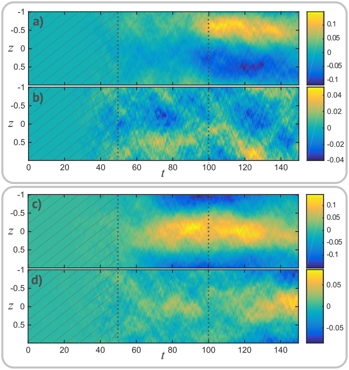
The formal applicability of statistical simulation is limited to low Rm due to the quasi-linear approximation. Our second method utilizes DNS, forced kinetically at small scales, to show that magnetic fields arising consistently through the small-scale dynamo can drive a coherent large-scale dynamo. To this end, we directly calculate transport coefficients from nonlinear simulation before and after the saturation of the small-scale dynamo. We use the incompressible MHD code SNOOPY [29], which uses the pseudo-spectral method and shearing periodic boundary conditions. The chosen Reynolds numbers [17] are moderate – small enough such that there is no self-sustaining turbulence in the absence of small-scale forcing (although effects may be similar even when this occurs [30]) – and ensembles of 100 simulations are run with shear , both with and without Keplerian rotation. At these parameters, the prevalence of the coherent large-scale dynamo depends on the realization (see Fig. 2), and it appears that the coherent effect cannot always overcome fluctuations in immediately after small-scale saturation, although the dynamo develops after a sufficiently long time [e.g., Fig. 2(d) near ]. This behavior seems generic when the coherent dynamo is close to its threshold for excitation and we have observed similar structures when the induction equation is driven directly at lower Rm [26]. Notwithstanding this variability in the dynamo’s qualitative behavior, measurement of the transport coefficients illustrates that the coefficient decreases after the magnetic fluctuations reach approximate equipartition with velocity fluctuations at small scales.
At low times, we use the test-field method to measure the kinematic and , fixing the mean field and calculating , with no Lorentz force [3, 18]. Since the small-scale dynamo grows quickly, test-fields are reset every . After small-scale saturation, standard test-field methods are inapplicable [31]. Instead, we extract and simulation data and calculate directly from Eq. (2) by computing for each of and solving the resulting matrix equations (in the least-squares sense) at each time point. This method is similar to that presented in Ref. [32]; however, we additionally impose the constraints , and . While these changes may appear to make the method less accurate, they in fact achieve the opposite by reducing the influence of . This is necessary because has a high level of noise in comparison to its magnitude, and because this noise is correlated with the noise in (due to directly driving ) and (through ). These correlations are very harmful to the quality of the fit, causing unphysical negative values for [32], which also pollute measurement of other coefficients. It is straightforward to show that the systematic errors caused by our constraints on the transport coefficients are less than for the dynamos in Fig. 2, so long as when time averaged. We have verified the method is accurate by comparison with the kinematic test-field method at low Rm, where there is no small-scale dynamo [33, 26] and the rotation can be used to explore a range of . In addition, the measurements are independently verified in Fig. 4 below 33 3 Ideally, one would utilize the same method to measure transport coefficients before and after small-scale saturation. However, the very fast growth of the small-scale field at early times renders the passive transport coefficient measurement unfeasible, since the mean field is dominated by small-scale fields and Eq. (2) does not apply.. Due to the short time-window, measurements of the transport coefficients after small-scale saturation vary significantly between realization, as should be expected from Fig. 2. Nonetheless, an average over the ensemble of 100 simulations illustrates a statistically significant change in that is consistent with observed behavior.
Results are illustrated in Fig. 3. In the kinematic phase without rotation, we see in qualitative agreement with previous studies [18]. With rotation , consistent with a reduction in due to the effect [5]. After saturation of the small-scale dynamo, for the non-rotating case, while in the rotating case – the same reduction in each to within error. Values for the diagonal resistivity are smaller after saturation, as expected since the velocity fluctuation energy decreases (by a factor ). The values of show that the dynamo is slightly stable on average in the non-rotating case and marginal in the rotating case. However, the coefficients vary significantly between realizations, sometimes yielding larger growth rates, and measurements match observed growth of the mean field for individual realizations. We illustrate this in Fig. 4, which demonstrates consistency between the measured transport coefficients and observed mean-field evolution by solving Eq. (3) directly [using the time-dependent (t) and ], for a sample of the rotating simulations. In addition, by artificially removing , we illustrate that cases with more negative are driven primarily by this, rather than a stochastic- effect. We thus conclude that small-scale magnetic fluctuations act to decrease , and that in some realizations (or after a sufficiently long time period) a coherent large-scale dynamo develops as a result.
To summarize, in this letter we have demonstrated that small-scale magnetic fluctuations, excited by small-scale dynamo action, can drive large-scale magnetic field generation. The mechanism is a magnetic analogue of the “shear-current” effect [16, 21], arising through the off-diagonal turbulent resistivity in the presence of large-scale shear flow. We have demonstrated its existence numerically using both DNS, with measurements of mean-field transport coefficients before and after small-scale dynamo saturation, and through quasi-linear statistical simulation.
More work is needed to precisely assess regimes in which the magnetically driven dynamo might dominate, as well as its behavior at higher Reynolds numbers where self-sustained turbulence is possible [30]. Another interesting question regards whether a magnetic dynamo can remain influential in the presence of net helicity and an effect, particularly as small-scale dynamo may be suppressed by shear [35]. While such questions may be difficult to answer definitively, the generic presence of magnetic fluctuations in plasma turbulence gives us some confidence that the proposed mechanism could cause large-scale dynamo growth in the wide variety of astrophysical systems with velocity shear.
Acknowledgements.
This work was supported by a Procter Fellowship at Princeton University, and the US Department of Energy Grant DE-AC02-09-CH11466. The authors would like to thank A. Schekochihin, J. Krommes, and I. Rogachevskii for enlightening discussion and useful suggestions.References
- [1] D. H. Hathaway, Living Reviews in Solar Physics 7, 1 (2010).
- [2] H. K. Moffatt, Magnetic Field Generation in Electrically Conducting Fluids (Cambridge University Press, 1978).
- [3] A. Brandenburg and K. Subramanian, Phys. Rep. 417, 1 (2005).
- [4] N. Yokoi, Geophys. Astrophys. Fluid Dyn. 107, 114 (2013).
- [5] F. Krause and K. H. Rädler, Mean-field magnetohydrodynamics and dynamo theory (Oxford: Pergamon Press, 1980).
- [6] R. M. Kulsrud and S. W. Anderson, Astrophys. J. 396, 606 (1992).
- [7] F. Cattaneo and D. W. Hughes, Mon. Not. R. Astron. Soc. 395, L48 (2009).
- [8] A. A. Schekochihin et al., New J. Phys. 9, 300 (2007).
- [9] S. Boldyrev, F. Cattaneo, and R. Rosner, Phys. Rev. Lett. 95, 255001 (2005).
- [10] A. V. Gruzinov and P. H. Diamond, Phys. Rev. Lett. 72, 1651 (1994).
- [11] A. Bhattacharjee and Y. Yuan, Astrophys. J. 449, 739 (1995).
- [12] E. G. Blackman and G. B Field, Phys. Rev. Lett. 89, 265007 (2002).
- [13] H. Hotta, M. Rempel, and T. Yokoyama, Astrophys. J. 803, 42 (2015).
- [14] J. Squire and A. Bhattacharjee, Phys. Rev. Lett. 114, 085002 (2015).
- [15] J. Squire and A. Bhattacharjee, (2015a), in preparation.
- [16] I. Rogachevskii and N. Kleeorin, Phys. Rev. E 70, 046310 (2004).
- [17] T. A. Yousef et al., Astron. Nachr. 329, 737 (2008a).
- [18] A. Brandenburg, K. H. Rädler, M. Rheinhardt, and P. J. Käpylä, Astrophys. J. 676, 740 (2008).
- [19] V. Urpin, Astron. Astrophys. 347, L47 (1999).
- [20] V. Urpin, Phys. Rev. E 65, 026301 (2002).
- [21] I. Rogachevskii and N. Kleeorin, Phys. Rev. E 68, 036301 (2003).
- [22] K.-H. Rädler and R. Stepanov, Phys. Rev. E 73, 056311 (2006).
- [23] N. K. Singh and S. Sridhar, Phys. Rev. E 83, 056309 (2011).
- [24] This condition may be altered if one considers the effects of magnetic helicity conservation, which may cause a local magnetic effect as the large-scale field grows [18]. However, this also causes coupling between different mean-field modes, and the detailed consequences of such an effect remain unclear.
- [25] Specifically, for the forcing (acting through and ), we keep constant (in the statistical sense) across all simulations in Fig. 1.
- [26] J. Squire and A. Bhattacharjee, ArXiv e-prints (2015b), arXiv:1507.03154 [astro-ph.HE] .
- [27] B. F. Farrell and P. J. Ioannou, J. Fluid Mech. 708, 149 (2012).
- [28] S. M. Tobias, K. Dagon, and J. B. Marston, Astrophys. J. 727, 127 (2011).
- [29] G. Lesur and P. Y. Longaretti, Mon. Not. R. Astron. Soc. 378, 1471 (2007).
- [30] G. Lesur and G. I. Ogilvie, Astron. Astrophys. 488, 451 (2008).
- [31] M. Rheinhardt and A. Brandenburg, Astron. Astrophys. 520, A28 (2010).
- [32] A. Brandenburg and D. Sokoloff, Geophys. Astrophys. Fluid Dyn. 96, 319 (2002).
- [33] T. A. Yousef et al., Phys. Rev. Lett. 100, 184501 (2008b).
- [34] Ideally, one would utilize the same method to measure transport coefficients before and after small-scale saturation. However, the very fast growth of the small-scale field at early times renders the passive transport coefficient measurement unfeasible, since the mean field is dominated by small-scale fields and Eq. (2) does not apply.
- [35] S. M. Tobias and F. Cattaneo, Nature 497, 463 (2014).