Adaptive Stochastic Primal-Dual Coordinate Descent for Separable Saddle Point Problems
Abstract
We consider a generic convex-concave saddle point problem with separable structure, a form that covers a wide-ranged machine learning applications. Under this problem structure, we follow the framework of primal-dual updates for saddle point problems, and incorporate stochastic block coordinate descent with adaptive stepsize into this framework. We theoretically show that our proposal of adaptive stepsize potentially achieves a sharper linear convergence rate compared with the existing methods. Additionally, since we can select “mini-batch” of block coordinates to update, our method is also amenable to parallel processing for large-scale data. We apply the proposed method to regularized empirical risk minimization and show that it performs comparably or, more often, better than state-of-the-art methods on both synthetic and real-world data sets.
Keywords:
large-scale optimization, parallel optimization, stochastic coordinate descent, convex-concave saddle point problems1 Introduction
The generic convex-concave saddle point problem is written as
| (1) |
where is a proper convex function, is the convex conjugate of a convex function , and matrix . Many machine learning tasks reduce to solving a problem of this form [6, 3]. As a result, this saddle problem has been widely studied [16, 14, 2, 1, 4, 5].
One important subclass of the general convex concave saddle point problem is where or exhibits an additive separable structure. We say is separable when , with , and . Separability for is defined likewise. To keep the consistent notation for the machine learning applications discussed later, we introduce matrix and let . Then we partition matrix into column blocks , , and , resulting in a problem of the form
| (2) |
for separable. We call any problem of the form (1) where or has separable structure, a Separable Convex Concave Saddle Point (Sep-CCSP) problem. Eq. (2) gives the explicit form for when is separable.
In this work, we further assume that each is -strongly convex, and is -strongly convex, i.e.,
where we use to denote both the gradient for smooth function and subgradient for non-smooth function. When the strong convexity cannot be satisfied, a small strongly convex perturbation can be added to make the problem satisfy the assumption [15].
One important instantiation of the Sep-CCSP problem in machine learning is the regularized empirical risk minimization (ERM, [3]) of linear predictors,
| (3) |
where are the feature vectors of data samples, corresponds the convex loss function w.r.t. the linear predictor , and is a convex regularization term. Many practical classification and regression models fall into this regularized ERM formulation, such as linear support vector machine (SVM), regularized logistic regression and ridge regression, see [3] for more details.
Reformulating the above regularized ERM by employing conjugate dual of the function , i.e.
| (4) |
leads directly to the following Sep-CCSP problem
| (5) |
Comparing with the general form, we note that the matrix in (2) is now a vector . For solving the general saddle point problem (1), many primal-dual algorithms can be applied, such as [16, 2, 1, 4, 5]. In addition, the saddle point problem we consider can also be formulated as a composite function minimization problem and then solved by Alternating Direction Method of Multipliers (ADMM) methods [9].
To handle the Sep-CCSP problem particularly for regularized ERM problem (5), Zhang and Xiao [15] proposed a stochastic primal-dual coordinate descent (SPDC) method. SPDC applies stochastic coordinate descent method [8, 10, 11] into the primal-dual framework, where in each iteration a random subset of dual coordinates are updated. This method inherits the efficiency of stochastic coordinate descent for solving large-scale problems. However, they use a conservative constant stepsize during the primal-dual updates, which leads to an unsatisfying convergence rate especially for unnormalized data.
In this work, we propose an adaptive stochastic primal-dual coordinate descent (AdaSPDC) method for solving the Sep-CCSP problem (2), which is a non-trivial extension of SPDC. By carefully exploiting the structure of individual subproblem, we propose an adaptive stepsize rule for both primal and dual updates according to the chosen subset of coordinate blocks in each iteration. Both theoretically and empirically, we show that AdaSPDC could yield a significantly better convergence performance than SPDC and other state-of-the-art methods.
The remaining structure of the paper is as follows. Section 2 summarizes the general primal-dual framework our method and SPDC are based on. Then we elaborate our method AdaSPDC in Section 3, where both the theoretical result and its comparison with SPDC are provided. In Section 4, we apply our method into regularized ERM tasks, and experiment with both synthetic and real-world datasets, and we show the superiority of AdaSPDC over other competitive methods empirically. Finally, Section 5 concludes the work.
2 Primal-dual Framework for Convex-Concave Saddle Point Problems
Chambolle and Pock [1] proposed a first-order primal-dual method for the CCSP problem (1). We refer this algorithm as PDCP. The update of PDCP in the th iteration is as follows:
| (6) | ||||
| (7) | ||||
| (8) |
When the parameter configuration satisfies and , PDCP could achieve convergence rate for general convex function and , where is total number of iterations. When and are both strongly convex, a linear convergence rate can be achieved by using a more scheduled stepsize. PDCP is a batch method and non-stochastic, i.e., it has to update all the dual coordinates in each iteration for Sep-CCSP problem, which will be computationally intensive for large-scale (high-dimensional) problems.
SPDC [15] can be viewed as a stochastic variant of the batch method PDCP for handling Sep-CCSP problem. However, SPDC uses a conservative constant stepsize for primal and dual updates. Both PDCP and SPDC do not consider the structure of matrix and only apply constant stepsize for all coordinates of primal and dual variables. This might limit their convergence performance in reality.
Based on this observation, we exploit the structure of matrix (i.e., ) and propose an adaptive stepsize rule for efficiently solving Sep-CCSP problem. A better linear convergence rate could be yielded when and are strongly convex. Our algorithm will be elaborated in the following section.
3 Adaptive Stochastic Primal-Dual Coordinate Descent
As a non-trivial extension of SPDC [15], our method AdaSPDC solves the Sep-CCSP problem (2) by using an adaptive parameter configuration. Concretely, we optimize by alternatively updating the dual and primal variables in a principled way. Thanks to the separable structure of , in each iteration we can randomly select blocks of dual variables whose indices are denoted as , and then we only update these selected blocks in the following way,
| (9) |
For those coordinates in blocks not selected, , we just keep . By exploiting the structure of individual , we configure the stepsize parameter of the proximal term adaptively
| (10) |
where , with is the spectral norm of a matrix and to denote the maximum singular value of a matrix.
Our step size is different from the one used in SPDC [15], where is a constant (since SPDC only considers ERM problem, the matrix is a feature vector ).
Remark. Intuitively, in AdaSPDC can be understood as the coupling strength between the -th dual variable block and primal variable, measured by the spectral norm of matrix . Smaller coupling strength allows us to use larger stepsize for the current dual variable block without caring too much about its influence on primal variable, and vice versa. Compared with SPDC, our proposal of an adaptive coupling strength for the chosen coordinate block directly results in larger step size, and thus helps to improve convergence speed.
In the stochastic dual update, we also use an intermediate variable as in PDCP algorithm, and we will describe its update later.
Since we assume is not separable, we update the primal variable as a whole,
| (11) |
The proximal parameter is also configured adaptively,
| (12) |
where , compared with constant used in SPDC. To account for the incremental change after the latest dual update, an auxiliary variable is used and updated as follows
| (13) |
Finally, we update the intermediate variable , which implements an extrapolation step over the current and can help to provide faster convergence rate [7, 1].
| (14) |
where is configured adaptively as
| (15) |
which is contrary to the constant used in SPDC.
The whole procedure for solving Sep-CCSP problem (2) using AdaSPDC is summarized in Algorithm 1. There are several notable characteristics of our algorithms.
- •
Compared with SPDC, our method uses adaptive step size to obtain faster convergence (will be shown in Theorem 3.1), while the whole algorithm does not bring any other extra computational complexity. As demonstrated in the experiment Section 4, in many cases, AdaSPDC provides significantly better performance than SPDC.
- •
Since, in each iteration, a number of block coordinates can be chosen and updated independently (with independent evaluation of individual step size), this directly enables parallel processing, and hence use on modern computing clusters. The ability to select an arbitrary number of blocks can help to make use of all the computation structure available as effectively as possible.
3.1 Convergence Analysis
We characterise the convergence performance of our method in the following theorem.
Theorem 3.1
Since the proof of the above is technical, we provide it in the Supplementary Material.
In our proof, given the proposed parameter , the critical point for obtaining a sharper linear convergence rate than SPDC is that we configure and as Eq. (12) and (10) to guarantee the positive definiteness of the following matrix in the -th iteration,
| (17) |
where and . However, we found that the parameter configuration to guarantee the positive definiteness of is not unique, and there exist other valid parameter configurations besides the proposed one in this work. We leave the further investigation on other potential parameter configurations as future work.
3.2 More Comparison with SDPC
Compared with SPDC [15], AdaSPDC follows the similar primal-dual framework. The crucial difference between them is that AdaSPDC proposes a larger stepsize for both dual and primal updates, see Eq. (10) and (12) compared with SPDC’s parameter configuration given in Eq.(10) in [15], where SPDC applies a large constant while AdaSPDC uses a more adaptive value of and for -th iteration to account for the different coupling strength between the selected dual coordinate block and primal variable. This difference directly means that AdaSPDC can potentially obtain a significantly sharper linear convergence rate than SPDC, since the decay factor of AdaSPDC is smaller than in SPDC (Eq.(10) in [15]) , see Theorem 3.1 for AdaSPDC compared with SPDC (Theorem 1 in [15]). The empirical performance of the two algorithms will be demonstrated in the experimental Section 4.
To mitigate the problem that SPDC uses a large , the authors of SPDC proposes to non-uniformly sample the the dual coordinate to update in each iteration according to the norm of the each . However, as we show later in the empirical experiments, this non-uniform sampling does not work very well for some datasets. By configuring the adaptive stepsize explicitly, our method AdaSPDC provides a better solution for unnormalized data compared with SPDC, see Section 4 for more empirical evidence.
Another difference is that SPDC only considers the regularized ERM task, i.e., only handling the case that each is a feature vector , while AdaSPDC extends that can be a matrix so that AdaSPDC can cover a wider range of applications than SPDC, i.e. in each iteration, a number of block coordinates could be selected while for SPDC only a number of coordinates are allowed.
 |
 |
| (a) | (b) |
 |
 |
| (c) | (d) |
4 Empirical Results
In this section, we appy AdaSPDC to several regularized empirical risk minimization problems. The experiments are conducted to compare our method AdaSPDC with other competitive stochastic optimization methods, including SDCA [13], SAG [12], SPDC with uniform sampling and non-uniform sampling [15]. In order to provide a fair comparison with these methods, in each iteration only one dual coordinate (or data instance) is chosen, i.e., we run all the methods sequentially. To obtain results that are independent of the practical implementation of the algorithm, we measure the algorithm performance in term of objective suboptimality w.r.t. the effective passes to the entire data set.
Each experiment is run 10 times and the average results are reported to show statistical consistency. We present all the experimental results we have done for each application.
4.1 Ridge Regression
We firstly apply our method AdaSPDC into a simple ridge regression problem with synthetic data. The data is generated in the same way as Zhang and Xiao [15]; i.i.d. training points are generated in the following manner,
where and , and the elements of the vector are all ones. The covariance matrix is set to be diagonal with , for . Then the ridge regression tries to solve the following optimization problem,
| (18) |
The optimal solution of the above ridge regression can be found as
By employing the conjugate dual of quadratic loss (crossref, Eq. (4)), we can reformulate the ridge regression as the following Sep-CCSP problem,
| (19) |
It is easy to figure out that is -strongly convex, and is -strongly convex.
Thus, for ridge regression, the dual update in Eq. (9) and primal update in Eq. (11) of AdaSPDC have closed form solutions as below,
The algorithm performance is evaluated in term of objective suboptimality (measured by ) w.r.t. number of effective passes to the entire datasets. Varying values of regularization parameter are experimented to demonstrate algorithm performance with different degree of ill-conditioning, .
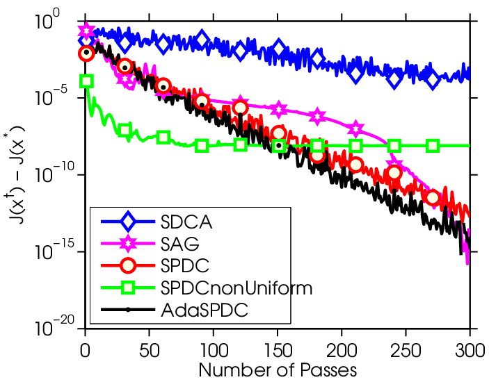
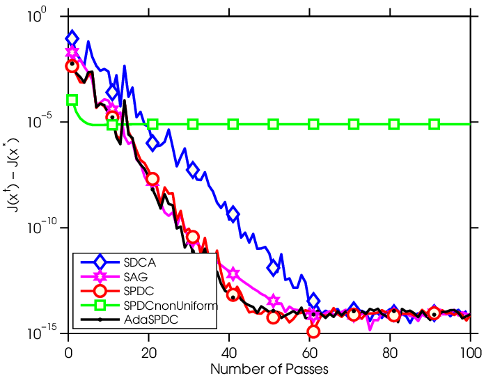
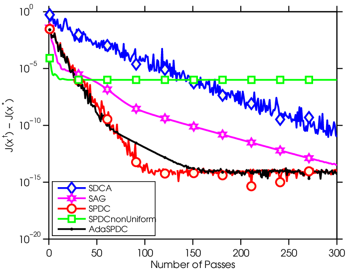
Fig. 1 shows algorithm performance with different degrees of regularization. It is easy to observe that AdaSPDC converges substantially faster than other compared methods, particularly for ill-conditioned problems. Compared with SPDC and its variant with non-uniform sampling, the usage of adaptive stepsize in AdaSPDC significantly improves convergence speed. For instance, in the case with , AdaSPDC achieves 100 times better suboptimality than both SPDC and its variant SPDC with non-uniform sampling after 300 passes.
| Datasets | Number of samples | Number of features | Sparsity |
|---|---|---|---|
| w8a | 49,749 | 300 | 3.9% |
| covertype | 20,242 | 47,236 | 0.16% |
| url | 2,396,130 | 3,231,961 | 0.0018% |
| quantum | 50,000 | 78 | 43.44% |
| protein | 145,751 | 74 | 99.21% |
| Dataset | |||
|---|---|---|---|
| w8a |  |
 |
 |
| covtype | 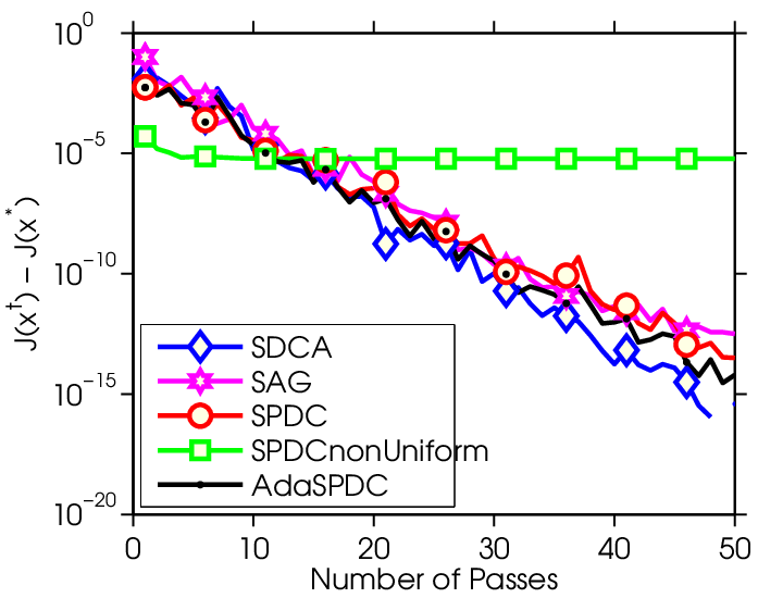 |
 |
 |
| url |  |
 |
 |
| quantum |  |
 |
 |
| protein |  |
 |
 |
| Dataset | |||
|---|---|---|---|
| w8a |  |
 |
 |
| covertype | 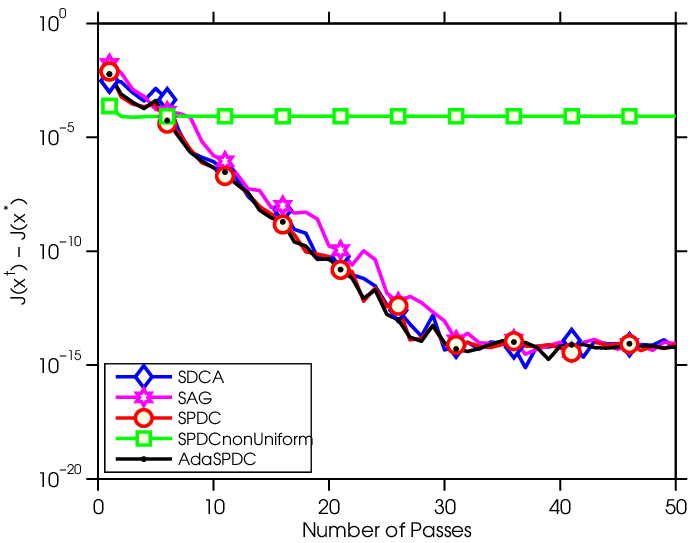 |
 |
 |
| url |  |
 |
 |
| quantum |  |
 |
 |
| protein |  |
 |
 |
4.2 Binary Classification on Real-world Datasets
We now compare the performance of our method AdaSPDC with other competitive methods on several real-world data sets. Our experiments focus on the freely-available benchmark data sets for binary classification, whose detailed information are listed in Table 1. The w8a, covertype and url data are obtained from the LIBSVM collection11 1 http://www.csie.ntu.edu.tw/~cjlin/libsvmtools/datasets/binary.html. The quantum and protein data sets are obtained from KDD Cup 200422 2 http://osmot.cs.cornell.edu/kddcup/datasets.html. For all the datasets, each sample takes the form with is the feature vector and is the binary label or . We add a bias term to the feature vector for all the datasets. We aim to minimize the regularized empirical risk with following form
| (20) |
To provide a more comprehensive comparison between these methods, we experiment with two different loss function , smooth Hinge loss [13] and logistic loss, described in the following.
Smooth Hinge loss
(with smoothing parameter .)
And its conjugate dual is
We can observe that is -strongly convex with . The dual update of AdaSPDC for smooth Hinge loss is nearly the same with ridge regression except the necessity of projection into the interval .
Logistic loss
whose conjugate dual has the form
It is also easy to obtain that is -strongly convex with . Note that for logistic loss, the dual update in Eq. (9) does not have a closed form solution, and we can start from some initial solution and further apply several steps of Newton’s update to obtain a more accurate solution.
During the experiments, we observe that the performance of SAG is very sensitive to the stepsize choice. To obtain best results of SAG, we try different choices of stepsize in the interval and report the best result for each dataset, where is Lipschitz constant of , is the theoretical stepsize choice for SAG and is the suggested empirical choice [12]. For smooth Hinge loss, , and for logistic loss, .
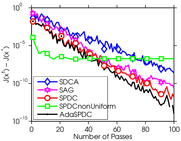
Fig. 2 and Fig. 3 depict the algorithm performance on the different methods with smooth Hinge loss and logistics loss, respectively. We compare all these methods with different values of . Generally, our method AdaSPDC performs consistently better or at least comparably with other methods, and performs especially well for the tasks with small regularized parameter . For some datasets, such as covertype and quantum, SPDC with non-uniform sampling decreases the objective faster than other methods in early epochs, however, cannot achieve comparable results with other methods in later epochs, which might be caused by its conservative stepsize.
5 Conclusion & Future Work
In this work, we propose Adaptive Stochastic Primal-Dual Coordinate Descent (AdaSPDC) for separable saddle point problems. As a non-trivial extension of a recent work SPDC [15], AdaSPDC uses an adaptive step size choices for both primal and dual updates in each iteration. The design of the step size for our method AdaSPDC explicitly and adaptively models the coupling strength between chosen block coordinates and primal variable through the spectral norm of each . We theoretically characterise that AdaSPDC holds a sharper linear convergence rate than SDPC. Additionally, we demonstrate the superiority of the proposed AdaSPDC method on ERM problems through extensive experiments on both synthetic and real-world data sets.
An immediate further research direction is to investigate other valid parameter configurations for the extrapolation parameter , and the primal and dual step sizes and both theoretically and empirically. In addition, discovering the potential theoretical connections with other stochastic optimization methods will also be enlightening.
Acknowledgments.
Z. Zhu is supported by China Scholarship Council/University of Edinburgh Joint Scholarship. The authors would like to thank Jinli Hu for insightful discussion on the proof of Theorem 1.
References
- [1] Chambolle, A., Pock, T.: A first-order primal-dual algorithm for convex problems with applications to imaging. Journal of Mathematical Imaging and Vision 40(1), 120–145 (2011)
- [2] Esser, E., Zhang, X., Chan, T.: A general framework for a class of first order primal-dual algorithms for convex optimization in imaging science. SIAM Journal on Imaging Sciences 3(4), 1015–1046 (2010)
- [3] Hastie, T., Tibshirani, R., Friedman, J.: The elements of statistical learning, vol. 2. Springer (2009)
- [4] He, B., Yuan, X.: Convergence analysis of primal-dual algorithms for a saddle-point problem: from contraction perspective. SIAM Journal on Imaging Sciences 5(1), 119–149 (2012)
- [5] He, Y., Monteiro, R.D.: An accelerated hpe-type algorithm for a class of composite convex-concave saddle-point problems. Optimization-online preprint (2014)
- [6] Jacob, L., Obozinski, G., Vert, J.P.: Group lasso with overlap and graph lasso. In: Proceedings of the 26th annual international conference on machine learning. pp. 433–440. ACM (2009)
- [7] Nesterov, Y.: Introductory lectures on convex optimization: A basic course, vol. 87. Springer (2004)
- [8] Nesterov, Y.: Efficiency of coordinate descent methods on huge-scale optimization problems. SIAM Journal on Optimization 22(2), 341–362 (2012)
- [9] Ouyang, Y., Chen, Y., Lan, G., Pasiliao Jr, E.: An accelerated linearized alternating direction method of multipliers. arXiv preprint arXiv:1401.6607 (2014)
- [10] Richtárik, P., Takáč, M.: Parallel coordinate descent methods for big data optimization. arXiv preprint arXiv:1212.0873 (2012)
- [11] Richtárik, P., Takáč, M.: Iteration complexity of randomized block-coordinate descent methods for minimizing a composite function. Mathematical Programming 144(1-2), 1–38 (2014)
- [12] Schmidt, M., Roux, N.L., Bach, F.: Minimizing finite sums with the stochastic average gradient. arXiv preprint arXiv:1309.2388 (2013)
- [13] Shalev-Shwartz, S., Zhang, T.: Stochastic dual coordinate ascent methods for regularized loss. The Journal of Machine Learning Research 14(1), 567–599 (2013)
- [14] Tseng, P.: On accelerated proximal gradient methods for convex-concave optimization. submitted to SIAM Journal on Optimization (2008)
- [15] Zhang, Y., Xiao, L.: Stochastic primal-dual coordinate method for regularized empirical risk minimization. arXiv preprint arXiv:1409.3257 (2014)
- [16] Zhu, M., Chan, T.: An efficient primal-dual hybrid gradient algorithm for total variation image restoration. UCLA CAM Report pp. 08–34 (2008)
Appendix: Proofs
Before presenting the proof of Theorem 1, we firstly provide the following lemma and its proof, which characterizes positive semi-definiteness of an important matrix used in the proof of Theorem 1.
Lemma 1
Given any matrix , we partition the matrix into column blocks, , , and then . We then define two diagonal matrices, , and and let . And denote , where is the spectral norm and is the maximum singular value of a matrix. And let . Now we consider the following parameter configuration, for any positive constant ,
| (21) | ||||
| (22) |
Under the above parameter configuration, the following matrix is positive definite,
| (23) |
Proof
Firstly consider each separable column block , then
| (24) |
For any , , we consider
| (25) |
Applying the Cauchy-Schwarz inequality and the fact that for any and , we obtain,
| (26) | ||||
| (27) |
In view of the inequality (24), it is obvious that there exists certain such that the following equality holds,
| (28) |
Thanks to this equality, now we set , and the inequality (27) can be further simplified,
| (29) | ||||
| (30) |
Let , and now we consider for any non-zero , the following inner product can be expanded,
| (31) |
Inserting the inequality (30) into the above equation, we obtain,
| (32) | ||||
| (33) | ||||
| (34) |
which guarantees the positive definiteness of the matrix .
Now we are ready to proof the Theorem 3.1 in our paper:
Proof
Firstly, we analyze the value of the dual variable after -th update in Algorithm 1. For any , let be the value of if , i.e.,
| (35) |
Since is -strongly convex, thus the function to be minimized above is -strongly convex. Then we have,
| (36) |
Since the is the saddle point, we can obtain following inequality,
| (37) |
Adding the two inequalities together, we have
| (38) |
In our algorithm, an index set is randomly chosen. For every specific index , the event happens with probability . If , then is updated to the value . Otherwise, is kept to be its old value . Let be the random event that contains the set of all random variable before round ,
| (39) |
and then we have
Consequently, we can insert the representations of , and in terms of the above expectations into the inequality (38),
| (40) |
Then we add the above inequality from , and divide both sides by , and obtain
| (41) |
where , , , and . In the crossing term between primal and dual variable, we use the fact that since only the blocks in index set are chosen and updated in -th update.
Now we characterize the -th update of primal variable . Following the same derivation for dual variable and using the assumption that is -strongly convex, we can easily obtain
| (42) |
Taking expectation over both sides of the above inequality and adding it to the the inequality (41), then we have
| (43) |
where the matrix .
Now we focus on the most crucial part of the proof: bounding the last term of R.H.S. of the above inequality (43). Firstly we rearrange this crossing term as follows,
| (44) |
Given the parameter configuration in Eq (12) and (10), we consider the following symmetric matrix,
| (45) |
Applying the Lemma 1, we can guarantee the positive definiteness of the matrix , which naturally leads the following inequality,
| (46) |
Similarly, we can also obtain
| (47) |
Taking the expectation for both sides of the above two equalities and using the facts that
we have that
| (48) |
Similarly, we can obtain
| (49) |
Therefore,
| (50) | ||||
| (51) |
Now we insert the Eq. (44) into the inequality (43), and then apply the two bounds (50) and (51), we have
| (52) |
Recall the configuration for in Eq. (15), the last term of R.H.S. of the above inequality is non-negative, and can be bounded away. Then we have the following,
| (53) |
According to the defined sequence , we have
| (54) |
According to the parameter configuration for , and , we can easily verify that
Combining these two inequalities with the inequality (53) and Eq. (54), we have
| (55) |
Consider , the above inequality implies
| (56) |
where
| (57) |
Consider the following matrix
| (58) |
Applying the Lemma 1 again, we can guarantee the positive definiteness of the matrix, which implies that
| (59) |
Taking expectation,
| (60) |
Thus,
| (61) |
Then combining the above inequality with inequality (56), we have
| (62) |
where , , and , which completes the proof.