Linear Response Methods for Accurate Covariance Estimates from Mean Field Variational Bayes
Abstract
Mean field variational Bayes (MFVB) is a popular posterior approximation method due to its fast runtime on large-scale data sets. However, a well known major failing of MFVB is that it underestimates the uncertainty of model variables (sometimes severely) and provides no information about model variable covariance. We generalize linear response methods from statistical physics to deliver accurate uncertainty estimates for model variables—both for individual variables and coherently across variables. We call our method linear response variational Bayes (LRVB). When the MFVB posterior approximation is in the exponential family, LRVB has a simple, analytic form, even for non-conjugate models. Indeed, we make no assumptions about the form of the true posterior. We demonstrate the accuracy and scalability of our method on a range of models for both simulated and real data.
1 Introduction
With increasingly efficient data collection methods, scientists are interested in quickly analyzing ever larger data sets. In particular, the promise of these large data sets is not simply to fit old models but instead to learn more nuanced patterns from data than has been possible in the past. In theory, the Bayesian paradigm yields exactly these desiderata. Hierarchical modeling allows practitioners to capture complex relationships between variables of interest. Moreover, Bayesian analysis allows practitioners to quantify the uncertainty in any model estimates—and to do so coherently across all of the model variables.
Mean field variational Bayes (MFVB), a method for approximating a Bayesian posterior distribution, has grown in popularity due to its fast runtime on large-scale data sets [4, 3, 6]. But a well known major failing of MFVB is that it gives underestimates of the uncertainty of model variables that can be arbitrarily bad, even when approximating a simple multivariate Gaussian distribution [11, 2, 20]. Also, MFVB provides no information about how the uncertainties in different model variables interact [23, 2, 17, 20].
By generalizing linear response methods from statistical physics [15, 14, 13, 19] to exponential family variational posteriors, we develop a methodology that augments MFVB to deliver accurate uncertainty estimates for model variables—both for individual variables and coherently across variables. In particular, as we elaborate in Section 2, when the approximating posterior in MFVB is in the exponential family, MFVB defines a fixed-point equation in the means of the approximating posterior, and our approach yields a covariance estimate by perturbing this fixed point. We call our method linear response variational Bayes (LRVB).
We provide a simple, intuitive formula for calculating the linear response correction by solving a linear system based on the MFVB solution (Section 2.2). We show how the sparsity of this system for many common statistical models may be exploited for scalable computation (Section 2.3). We demonstrate the wide applicability of LRVB by working through a diverse set of models to show that the LRVB covariance estimates are nearly identical to those produced by a Markov Chain Monte Carlo (MCMC) sampler, even when MFVB variance is dramatically underestimated (Section 3). Finally, we focus in more depth on models for finite mixtures of multivariate Gaussians (Section 3.3), which have historically been a sticking point for MFVB covariance estimates [2, 20]. We show that LRVB can give accurate covariance estimates orders of magnitude faster than MCMC (Section 3.3). We demonstrate both theoretically and empirically that, for this Gaussian mixture model, LRVB scales linearly in the number of data points and approximately cubically in the dimension of the parameter space (Section 3.4).
Previous Work.
Linear response methods originated in the statistical physics literature [13, 19, 8, 14]. These methods have been applied to find new learning algorithms for Boltzmann machines [8], covariance estimates for discrete factor graphs [24], and independent component analysis [7]. [18] states that linear response methods could be applied to general exponential family models but works out details only for Boltzmann machines. [14], which is closest in spirit to the present work, derives general linear response corrections to variational approximations; indeed, the authors go further to formulate linear response as the first term in a functional Taylor expansion to calculate full pairwise joint marginals. However, it may not be obvious to the practitioner how to apply the general formulas of [14]. Our contributions in the present work are (1) the provision of concrete, straightforward formulas for covariance correction that are fast and easy to compute, (2) demonstrations of the success of our method on a wide range of new models, and (3) an accompanying suite of code.
2 Linear response covariance estimation
2.1 Variational Inference
Suppose we observe data points, denoted by the -long column vector , and denote our unobserved model parameters by . Here, is a column vector residing in some space ; it has subgroups and total dimension . Our model is specified by a distribution of the observed data given the model parameters—the likelihood —and a prior distributional belief on the model parameters . Bayes’ Theorem yields the posterior .
Mean-field variational Bayes (MFVB) approximates by a factorized distribution of the form . is chosen so that the Kullback-Liebler divergence between and is minimized. Equivalently, is chosen so that , for (the expected log posterior) and (the entropy of the variational distribution), is maximized:
| (1) |
Up to a constant in , the objective is sometimes called the “evidence lower bound”, or the ELBO [2]. In what follows, we further assume that our variational distribution, , is in the exponential family with natural parameter and log partition function : (expressed with respect to some base measure in ). We assume that is expressed with respect to the same base measure in as for . Below, we will make only mild regularity assumptions about the true posterior and no assumptions about its form.
If we assume additionally that the parameters at the optimum are in the interior of the feasible space, then may instead be described by the mean parameterization: with . Thus, the objective can be expressed as a function of , and the first-order condition for the optimality of becomes the fixed point equation
| (2) |
2.2 Linear Response
Let denote the covariance matrix of under the variational distribution , and let denote the covariance matrix of under the true posterior, :
In MFVB, may be a poor estimator of , even when , i.e., when the marginal estimated means match well [23, 2, 20]. Our goal is to use the MFVB solution and linear response methods to construct an improved estimator for . We will focus on the covariance of the natural sufficient statistic , though the covariance of functions of can be estimated similarly (see Appendix A).
The essential idea of linear response is to perturb the first-order condition around its optimum. In particular, define the distribution as a log-linear perturbation of the posterior:
| (3) |
where is a constant in . We assume that is a well-defined distribution for any in an open ball around 0. Since normalizes , it is in fact the cumulant-generating function of , so the derivatives of evaluated at give the cumulants of . To see why this perturbation may be useful, recall that the second cumulant of a distribution is the covariance matrix, our desired estimand:
The practical success of MFVB relies on the fact that its estimates of the mean are often good in practice. So we assume that , where is the mean parameter characterizing and is the MFVB approximation to . (We examine this assumption further in Section 3.) Taking derivatives with respect to on both sides of this mean approximation and setting yields
| (4) |
where we call the linear response variational Bayes (LRVB) estimate of the posterior covariance of .
We next show that there exists a simple formula for . Recalling the form of the KL divergence (see Eq. (1)), we have that . Then by Eq. (2), we have for . It follows from the chain rule that
| (5) |
where is the identity matrix. If we assume that we are at a strict local optimum and so can invert the Hessian of , then evaluating at yields
| (6) |
where we have used the form for in Eq. (2). So the LRVB estimator is the negative inverse Hessian of the optimization objective, , as a function of the mean parameters. It follows from Eq. (6) that is both symmetric and positive definite when the variational distribution is at least a local maximum of .
We can further simplify Eq. (6) by using the exponential family form of the variational approximating distribution . For in exponential family form as above, the negative entropy is dual to the log partition function [22], so ; hence,
Recall that for exponential families, . So Eq. (6) becomes11 1 For a comparison of this formula with the frequentist “supplemented expectation-maximization” procedure see Appendix C.
| (7) |
When the true posterior is in the exponential family and contains no products of the variational moment parameters, then and . In this case, the mean field assumption is correct, and the LRVB and MFVB covariances coincide at the true posterior covariance. Furthermore, even when the variational assumptions fail, as long as certain mean parameters are estimated exactly, then this formula is also exact for covariances. E.g., notably, MFVB is well-known to provide arbitrarily bad estimates of the covariance of a multivariate normal posterior [11, 23, 2, 20], but since MFVB estimates the means exactly, LRVB estimates the covariance exactly (see Appendix B).
2.3 Scaling the matrix inverse
Eq. (7) requires the inverse of a matrix as large as the parameter dimension of the posterior , which may be computationally prohibitive. Suppose we are interested in the covariance of parameter sub-vector , and let denote the remaining parameters: . We can partition Similar partitions exist for and . If we assume a mean-field factorization , then . (The variational distributions may factor further as well.) We calculate the Schur complement of in Eq. (7) with respect to its th component to find that
| (8) |
Here, and refer to - and -sized identity matrices, respectively. In cases where can be efficiently calculated (e.g., all the experiments in Section 3; see Fig. (5) in Appendix D), Eq. (8) requires only an -sized inverse.
3 Experiments
We compare the covariance estimates from LRVB and MFVB in a range of models, including models both with and without conjugacy 22 2 All the code is available on our Github repository, rgiordan/LinearResponseVariationalBayesNIPS2015, . We demonstrate the superiority of the LRVB estimate to MFVB in all models before focusing in on Gaussian mixture models for a more detailed scalability analysis.
For each model, we simulate datasets with a range of parameters. In the graphs, each point represents the outcome from a single simulation. The horizontal axis is always the result from an MCMC procedure, which we take as the ground truth. As discussed in Section 2.2, the accuracy of the LRVB covariance for a sufficient statistic depends on the approximation . In the models to follow, we focus on regimes of moderate dependence where this is a reasonable assumption for most of the parameters (see Section 3.2 for an exception). Except where explicitly mentioned, the MFVB means of the parameters of interest coincided well with the MCMC means, so our key assumption in the LRVB derivations of Section 2 appears to hold.
3.1 Normal-Poisson model
Model.
First consider a Poisson generalized linear mixed model, exhibiting non-conjugacy. We observe Poisson draws and a design vector , for . Implicitly below, we will everywhere condition on the , which we consider to be a fixed design matrix. The generative model is:
| (9) | ||||
For MFVB, we factorize . Inspection reveals that the optimal will be Gaussian, and the optimal will be gamma (see Appendix D). Since the optimal does not take a standard exponential family form, we restrict further to Gaussian . There are product terms in (for example, the term ), so , and the mean field approximation does not hold; we expect LRVB to improve on the MFVB covariance estimate. A detailed description of how to calculate the LRVB estimate can be found in Appendix D.
Results.
We simulated datasets, each with data points and a randomly chosen value for and . We drew the design matrix from a normal distribution and held it fixed throughout. We set prior hyperparameters , , and . To get the “ground truth” covariance matrix, we took draws from the posterior with the R MCMCglmm package [5], which used a combination of Gibbs and Metropolis Hastings sampling. Our LRVB estimates used the autodifferentiation software JuMP [10].
Results are shown in Fig. (1). Since is high in many of the simulations, and are correlated, and MFVB underestimates the standard deviation of and . LRVB matches the MCMC standard deviation for all , and matches for in all but the most correlated simulations. When gets very high, the MFVB assumption starts to bias the point estimates of , and the LRVB standard deviations start to differ from MCMC. Even in that case, however, the LRVB standard deviations are much more accurate than the MFVB estimates, which underestimate the uncertainty dramatically. The final plot shows that LRVB estimates the covariances of with , , and reasonably well, while MFVB considers them independent.


3.2 Linear random effects
Model.
Next, we consider a simple random slope linear model, with full details in Appendix E. We observe scalars and and a vector , for . Implicitly below, we will everywhere condition on all the and , which we consider to be fixed design matrices. In general, each random effect may appear in multiple observations, and the index indicates which random effect, , affects which observation, . The full generative model is:
We assume the mean-field factorization . Since this is a conjugate model, the optimal will be in the exponential family with no additional assumptions.
Results.
We simulated datasets of datapoints each and distinct random effects. We set prior hyperparameters to , , , , and . Our was 2-dimensional. As in Section 3.1, we implemented the variational solution using the autodifferentiation software JuMP [10]. The MCMC fit was performed with using MCMCglmm [5].
Intuitively, when the random effect explanatory variables are highly correlated with the fixed effects , then the posteriors for and will also be correlated, leading to a violation of the mean field assumption and an underestimated MFVB covariance. In our simulation, we used , so that is correlated with but not . The result, as seen in Fig. (2), is that is underestimated by MFVB, but is not. The parameter, in contrast, is not well-estimated by the MFVB approximation in many of the simulations. Since the LRVB depends on the approximation , its LRVB covariance is not accurate either (Fig. (2)). However, LRVB still improves on the MFVB standard deviation.


3.3 Mixture of normals
Model.
Mixture models constitute some of the most popular models for MFVB application [4, 3] and are often used as an example of where MFVB covariance estimates may go awry [2, 20]. Thus, we will consider in detail a Gaussian mixture model (GMM) consisting of a -component mixture of -dimensional multivariate normals with unknown component means, covariances, and weights. In what follows, the weight is the probability of the th component, is the -dimensional mean of the th component, and is the precision matrix of the th component (so is the covariance parameter). is the number of data points, and is the th observed -dimensional data point. We employ the standard trick of augmenting the data generating process with the latent indicator variables , for and , such that implies . So the generative model is:
| (10) |
We used diffuse conditionally conjugate priors (see Appendix F for details). We make the variational assumption . We compare the accuracy and speed of our estimates to Gibbs sampling on the augmented model (Eq. (10)) using the function rnmixGibbs from the R package bayesm. We implemented LRVB in C++, making extensive use of RcppEigen [1]. We evaluate our results both on simulated data and on the MNIST data set [9].
Results.
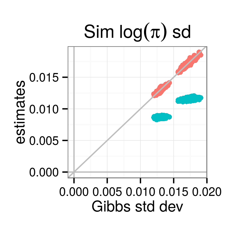
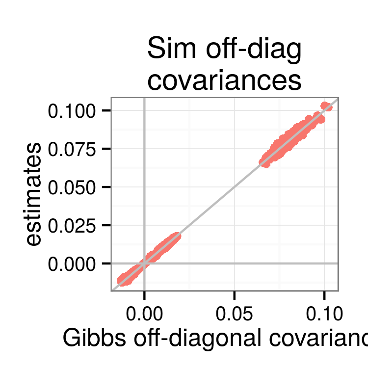
For simulations, we generated data points from multivariate normal components in dimensions. MFVB is expected to underestimate the marginal variance of , , and when the components overlap since that induces correlation in the posteriors due to the uncertain classification of points between the clusters. We check the covariances estimated with Eq. (7) against a Gibbs sampler, which we treat as the ground truth.33 3 The likelihood described in Section 3.3 is symmetric under relabeling. When the component locations and shapes have a real-life interpretation, the researcher is generally interested in the uncertainty of , , and for a particular labeling, not the marginal uncertainty over all possible re-labelings. This poses a problem for standard MCMC methods, and we restrict our simulations to regimes where label switching did not occur in our Gibbs sampler. The MFVB solution conveniently avoids this problem since the mean field assumption prevents it from representing more than one mode of the joint posterior.
We performed simulations, each of which had at least effective Gibbs samples in each variable—calculated with the R tool effectiveSize from the coda package [16]. The first three plots show the diagonal standard deviations, and the third plot shows the off-diagonal covariances. Note that the off-diagonal covariance plot excludes the MFVB estimates since most of the values are zero. Fig. (3) shows that the raw MFVB covariance estimates are often quite different from the Gibbs sampler results, while the LRVB estimates match the Gibbs sampler closely.
For a real-world example, we fit a GMM to the instances of handwritten s and s in the MNIST data set. We used PCA to reduce the pixel intensities to dimensions. Full details are provided in Appendix G. In this MNIST analysis, the standard deviations were under-estimated by MFVB but correctly estimated by LRVB (Fig. (3)); the other parameter standard deviations were estimated correctly by both and are not shown.



3.4 Scaling experiments
We here explore the computational scaling of LRVB in more depth for the finite Gaussian mixture model (Section 3.3). In the terms of Section 2.3, includes the sufficient statistics from , , and , and grows as . The sufficient statistics for the variational posterior of contain the -length vectors , for each , and the second-order products in the covariance matrix . Similarly, for each , the variational posterior of involves the sufficient statistics in the symmetric matrix as well as the term . The sufficient statistics for the posterior of are the terms .44 4 Since , using sufficient statistics involves one redundant parameter. However, this does not violate any of the necessary assumptions for Eq. (7), and it considerably simplifies the calculations. Note that though the perturbation argument of Section 2 requires the parameters of to be in the interior of the feasible space, it does not require that the parameters of be interior. So, minimally, Eq. (7) will require the inverse of a matrix of size . The sufficient statistics for have dimension . Though the number of parameters thus grows with the number of data points, for the multivariate normal (see Appendix F), so we can apply Eq. (8) to replace the inverse of an -sized matrix with multiplication by the same matrix. Since a matrix inverse is cubic in the size of the matrix, the worst-case scaling for LRVB is then in , in , and in .
In our simulations (Fig. (4)) we can see that, in practice, LRVB scales linearly55 5 The Gibbs sampling time was linearly rescaled to the amount of time necessary to achieve 1000 effective samples in the slowest-mixing component of any parameter. Interestingly, this rescaling leads to increasing efficiency in the Gibbs sampling at low due to improved mixing, though the benefits cease to accrue at moderate dimensions. in and approximately cubically in across the dimensions considered.66 6 For numeric stability we started the optimization procedures for MFVB at the true values, so the time to compute the optimum in our simulations was very fast and not representative of practice. On real data, the optimization time will depend on the quality of the starting point. Consequently, the times shown for LRVB are only the times to compute the LRVB estimate. The optimization times were on the same order. The scaling is presumably better than the theoretical worst case of due to extra efficiency in the numerical linear algebra. Note that the vertical axis of the leftmost plot is on the log scale. At all the values of , and considered here, LRVB was at least as fast as Gibbs sampling and often orders of magnitude faster.


4 Conclusion
The lack of accurate covariance estimates from the widely used mean-field variational Bayes (MFVB) methodology has been a longstanding shortcoming of MFVB. We have demonstrated that in sparse models, our method, linear response variational Bayes (LRVB), can correct MFVB to deliver these covariance estimates in time that scales linearly with the number of data points. Furthermore, we provide an easy-to-use formula for applying LRVB to a wide range of inference problems. Our experiments on a diverse set of models have demonstrated the efficacy of LRVB, and our detailed study of scaling of mixtures of multivariate Gaussians shows that LRVB can be considerably faster than traditional MCMC methods. We hope that in future work our results can be extended to more complex models, including Bayesian nonparametric models, where MFVB has proven its practical success.
Acknowledgments.
The authors thank Alex Blocker for helpful comments. R. Giordano and T. Broderick were funded by Berkeley Fellowships.
References
- [1] D. Bates and D. Eddelbuettel. Fast and elegant numerical linear algebra using the RcppEigen package. Journal of Statistical Software, 52(5):1–24, 2013.
- [2] C. M. Bishop. Pattern Recognition and Machine Learning. Springer, New York, 2006. Chapter 10.
- [3] D. M. Blei and M. I. Jordan. Variational inference for Dirichlet process mixtures. Bayesian Analysis, 1(1):121–143, 2006.
- [4] D. M. Blei, A. Y. Ng, and M. I. Jordan. Latent Dirichlet allocation. Journal of Machine Learning Research, 3:993–1022, 2003.
- [5] J. D. Hadfield. MCMC methods for multi-response generalized linear mixed models: The MCMCglmm R package. Journal of Statistical Software, 33(2):1–22, 2010.
- [6] M. D. Hoffman, D. M. Blei, C. Wang, and J. Paisley. Stochastic variational inference. Journal of Machine Learning Research, 14(1):1303–1347, 2013.
- [7] P. A. d. F. R. Højen-Sørensen, O. Winther, and L. K. Hansen. Mean-field approaches to independent component analysis. Neural Computation, 14(4):889–918, 2002.
- [8] H. J. Kappen and F. B. Rodriguez. Efficient learning in Boltzmann machines using linear response theory. Neural Computation, 10(5):1137–1156, 1998.
- [9] Y. LeCun, L. Bottou, Y. Bengio, and P. Haffner. Gradient-based learning applied to document recognition. Proceedings of the IEEE, 86(11):2278–2324, 1998.
- [10] M. Lubin and I. Dunning. Computing in operations research using Julia. INFORMS Journal on Computing, 27(2):238–248, 2015.
- [11] D. J. C. MacKay. Information Theory, Inference, and Learning Algorithms. Cambridge University Press, 2003. Chapter 33.
- [12] X. L. Meng and D. B. Rubin. Using EM to obtain asymptotic variance-covariance matrices: The SEM algorithm. Journal of the American Statistical Association, 86(416):899–909, 1991.
- [13] M. Opper and D. Saad. Advanced mean field methods: Theory and practice. MIT press, 2001.
- [14] M. Opper and O. Winther. Variational linear response. In Advances in Neural Information Processing Systems, 2003.
- [15] G. Parisi. Statistical Field Theory, volume 4. Addison-Wesley New York, 1988.
- [16] M. Plummer, N. Best, K. Cowles, and K. Vines. CODA: Convergence diagnosis and output analysis for MCMC. R News, 6(1):7–11, 2006.
- [17] H. Rue, S. Martino, and N. Chopin. Approximate Bayesian inference for latent Gaussian models by using integrated nested Laplace approximations. Journal of the Royal Statistical Society: Series B (statistical methodology), 71(2):319–392, 2009.
- [18] T. Tanaka. Mean-field theory of Boltzmann machine learning. Physical Review E, 58(2):2302, 1998.
- [19] T. Tanaka. Information geometry of mean-field approximation. Neural Computation, 12(8):1951–1968, 2000.
- [20] R. E. Turner and M. Sahani. Two problems with variational expectation maximisation for time-series models. In D. Barber, A. T. Cemgil, and S. Chiappa, editors, Bayesian Time Series Models. Cambridge University Press, 2011.
- [21] A. Wächter and L. T. Biegler. On the implementation of an interior-point filter line-search algorithm for large-scale nonlinear programming. Mathematical Programming, 106(1):25–57, 2006.
- [22] M. J. Wainwright and M. I. Jordan. Graphical models, exponential families, and variational inference. Foundations and Trends® in Machine Learning, 1(1-2):1–305, 2008.
- [23] B. Wang and M. Titterington. Inadequacy of interval estimates corresponding to variational Bayesian approximations. In Workshop on Artificial Intelligence and Statistics, pages 373–380, 2004.
- [24] M. Welling and Y. W. Teh. Linear response algorithms for approximate inference in graphical models. Neural Computation, 16(1):197–221, 2004.
You can find this paper, as well as all the code necessary to run the described experiments, in our Github repo, rgiordan/LinearResponseVariationalBayesNIPS2015.
Appendix A LRVB estimates of the covariance of functions
In Section 2.2, we derived an estimate of the covariance of the natural sufficient statistics, , of our variational approximation, . In this section we derive a version of Eq. (7) for the covariance of functions of .
We begin by estimating the covariance between and a function . Suppose we have an MFVB solution, , to Eq. (1). Define the expectation of to be . This expectation is function of alone since completely parameterizes . As in Eq. (3), we can consider a perturbed log likelihood that also includes :
Using the same reasoning that led to Eq. (4), we will define
We then have the following lemma:
Lemma A.1.
If is a differentiable function of with gradient , then
Proof.
The derivative of the perturbed ELBO, , is given by:
The fixed point Eq. (2) then gives:
The term is awkward, but it disappears when we evaluate at , giving
Recalling that
We can plug in to see that
| (18) |
∎
Finally, suppose we are interested in estimating , where . Again using the same reasoning that led to Eq. (4), we will define
Proposition A.2.
If and are differentiable functions of with gradients and respectively, then
Proof.
Appendix B Exactness of LRVB for multivariate normal means
For any target distribution , it is well-known that MFVB cannot be used to estimate the covariances between the components of . In particular, if is the estimate of returned by MFVB, will have a block-diagonal covariance matrix—no matter the form of the covariance of .
Consider approximating a multivariate Gaussian posterior distribution with MFVB. The Gaussian is the unique distribution that is fully determined by its mean and covariance. This posterior arises, for instance, given a multivariate normal likelihood with fixed covariance and an improper uniform prior on the mean parameter . We make the mean field factorization assumption , where is the total dimension of . This fact is often used to illustrate the shortcomings of MFVB [23, 2, 20]. In this case, it is well known that the MFVB posterior means are correct, but the marginal variances are underestimated if is not diagonal. However, since the posterior means are correctly estimated, the LRVB approximation in Eq. (7) is in fact an equality. That is, for this model, exactly.
In order to prove this result, we will rely on the following lemma.
Lemma B.1.
Consider a target posterior distribution characterized by , where and may depend on , and is invertible. Let , and consider a MFVB approximation to that factorizes as . Then the variational posterior means are the true posterior means; i.e. for all between and .
Proof.
The derivation of MFVB for the multivariate normal can be found in Section 10.1.2 of [2]; we highlight some key results here. Let . Let the index on a row or column correspond to , and let the index correspond to . E.g., for ,
By the assumption that , we have
| (19) | |||||
where the final term is constant with respect to . It follows that
So
with mean parameters
| (20) |
as well as an equation for .
Note that must be invertible, for if it were not, would not be invertible.
The solution is a unique stable point for Eq. (20), since the fixed point equations for each can be stacked and rearranged to give
The last step follows from the assumption that (and hence ) is invertible. It follows that is the unique stable point of Eq. (20).
∎
Proposition B.2.
Assume we are in the setting of Lemma B.1, where additionally and are on the interior of the feasible parameter space. Then the LRVB covariance estimate exactly captures the true covariance, .
Proof.
Consider the perturbation for LRVB defined in Eq. (3). By perturbing the log likelihood, we change both the true means and the variational solutions, . The result is a valid density function since the original and are on the interior of the parameter space. By Lemma B.1, the MFVB solutions are exactly the true means, so , and the derivatives are the same as well. This means that the first term in Eq. (7) is not approximate, i.e.
It follows from the arguments above that the LRVB covariance matrix is exact, and .
∎
Appendix C Comparison with supplemented expectation-maximization
The result in Appendix B about the multivariate normal distribution draws a connection between LRVB corrections and the “supplemented expectation-maximization” (SEM) method of [12]. SEM is an asymptotically exact covariance correction for the EM algorithm that transforms the full-data Fisher information matrix into the observed-data Fisher information matrix using a correction that is formally similar to Eq. (7). In this section, we argue that this similarity is not a coincidence; in fact the SEM correction is an asymptotic version of LRVB with two variational blocks, one for the missing data and one for the unknown parameters.
Although LRVB as described here requires a prior (unlike SEM, which supplements the MLE), the two covariance corrections coincide when the full information likelihood is approximately log quadratic and proportional to the posterior, . This might be expected to occur when we have a large number of independent data points informing each parameter—i.e., when a central limit theorem applies and the priors do not affect the posterior. In the full information likelihood, some terms may be viewed as missing data, whereas in the Bayesian model the same terms may be viewed as latent parameters, but this does not prevent us from formally comparing the two methods.
We can draw a term-by-term analogy with the equations in [12]. We denote variables from the SEM paper with a superscript “” to avoid confusion. MFVB does not differentiate between missing data and parameters to be estimated, so our corresponds to in [12]. SEM is an asymptotic theory, so we may assume that have a multivariate normal distribution, and that we are interested in the mean and covariance of .
In the E-step of [12], we replace with its conditional expectation given the data and other . This corresponds precisely to Eq. (20), taking . In the M-step, we find the maximum of the log likelihood with respect to , keeping fixed at its expectation. Since the mode of a multivariate normal distribution is also its mean, this, too, corresponds to Eq. (20), now taking .
It follows that the MFVB and EM fixed point equations are the same; i.e., our is the same as their , and our of Eq. (5) corresponds to the transpose of their , defined in Eq. (2.2.1) of [12]. Since the “complete information” corresponds to the variance of with fixed values for , this is the same as our , the variational covariance, whose inverse is . Taken all together, this means that equation (2.4.6) of [12] can be re-written as our Eq. (7).
Appendix D Normal-Poisson details
In this section, we use this model to provide a detailed, step-by-step description of a simple LRVB analysis.
The full joint distribution for the model in Eq. (9) is
We find a mean-field approximation under the factorization . By inspection, the log joint is quadratic in , so the optimal will be Gaussian [2]. Similarly, the log joint is a function of only via and , so the optimal will be gamma. However, the joint does not take a standard exponential family form in :
The difficulty is with the term . So we make the further restriction that
Fortunately, the troublesome term has an analytic expectation, as a function of the mean parameters, under this variational posterior:
We can now write the variational distribution in terms of the following mean parameters:
Calculating the LRVB covariance consists of roughly four steps:
- 1.
finding the MFVB optimum ,
- 2.
computing the covariance of ,
- 3.
computing , the Hessian of , for , and
- 4.
computing the matrix inverse and solving .
For step (1), the LRVB correction is agnostic as to how the optimum is found. In our experiments below, we follow a standard coordinate ascent procedure for MFVB [2]. We analytically update and . Given and , finding the optimal becomes separate two-dimensional optimization problems; there is one dimension for each of the mean parameters and . In our examples, we solved these problems sequentially using IPOPT [21].
To compute for step (2), we note that by the mean-field assumption, , , and are independent, so is block diagonal. Since we have chosen convenient variational distributions, the mean parameters have known covariance matrices. For example, from standard properties of the normal distribution, .
For step (3), the mean parameters for and co-occur with each other and with all the , so these four rows of are expected to be dense. However, the mean parameters for never occur with each other, so the bulk of —the block corresponding to the mean parameters of —will be block diagonal (Fig. (5(b))). The Hessian of can be calculated analytically, but we used the autodifferentiation software JuMP [10].
Finally, for step (4), we use the technique in Section 2.3 to exploit the sparsity of and (Fig. (5(c))) in calculating .


Appendix E Random effects model details
As introduced in Section 3.2, our model is:
With the priors:
We will make the following mean field assumption:
We have , and , and matches an observation to a random effect , allowing repeated observations of a random effect. The full joint log likelihood is:
Expanding the first term of the conditional likelihood of gives
By grouping terms, we can see that the mean parameters will be
It follows that the optimal variational distributions are multivariate normal, univariate normal, and and will be gamma. We performed standard coordinate ascent on these distributions [2].
As in Section 3.1, we implemented this model in the autodifferentiation software JuMP [10]. This means conjugate coordinate updates were easy, since the natural parameters corresponding to a mean parameters are the first derivatives of the log likelihood with respect to the mean parameters. For example, denoting the log likelihood at step by , the update for will be:
Given the partial derivatives of with respect to the mean parameters, the updated mean parameters for can be read off directly using standard properties of the normal distribution.
The variational covariance matrices are all standard. We can see that will have nonzero terms in general (for example, the three-way interaction ), and that LRVB will be different from MFVB. As usual in our models, is sparse, and we can easily apply the technique in section Section 2.3 to get the covariance matrix excluding the random effects, .
Appendix F Multivariate normal mixture details
In this section we derive the basic formulas needed to calculate Eq. (7) for a finite mixture of normals, which is the model used in Section 3. We will follow the notation introduced in Section 3.3.
Let each observation, , be a vector. We will denote the th component of the th observation , with a similar pattern for and . We will denote the , th entry in the matrix as . The data generating process is as follows:
It follows that the log posterior is given by
We used a multivariate normal prior for , a Wishart prior for , and a Dirichlet prior for . In the simulations described in Section 3.3, we used the following prior parameters for the VB model:
Here, is a -dimensional diagonal matrix with on the diagonal, and is a length vector of the value , with a similar definition for . Unfortunately, the function we used for the MCMC calculations, rnmixGibbs in the package bayesm, uses a different form for the prior. Specifically, rnmixGibbs uses the prior
where is a scalar. There is no way to exactly match to , so we simply set . Since our datasets are all reasonably large, the prior was dominated by the likelihood, and we found the results extremely insensitive to the prior on , so this discrepancy is of no practical importance.
The parameters , , , and will each be given their own variational distribution. For we will use a multivariate normal distribution; for we will us a Wishart distirbution; for we will use a Dirichlet distribution; for we will use a Multinoulli (a single multinomial draw). These are all the optimal variational choices given the mean field assumption and the conditional conjugacy in the model.
The sufficient statistics for are all terms of the form and . Consequently, the sub-vector of corresponding to is
We will only save one copy of and , so has length . For all the parameters, we denote the complete stacked vector without a subscript:
The sufficient statistics for are all the terms and the term . Again, since is symmetric, we do not keep redundant terms, so has length . The sufficient statistic for is the -vector . The sufficient statistics for are simply the values themselves.
In terms of Section 2.3, we have
That is, we are primarily interested in the covariance of the sufficient statistics of , , and . The latent variables are nuisance parameters.
To put the log likelihood in terms useful for LRVB, we must express it in terms of the sufficient statistics, taking into account the fact the vector does not store redundant terms (e.g. it will only keep for since is symmetric).
The MFVB updates and covariances in are all given by properties of standard distributions. To compute the LRVB corrections, it only remains to calculate the Hessian, . These terms can be read directly off the posterior. First we calculate derivatives with respect to components of .
All other derivatives are zero. For ,
The remaining derivatives are zero. The only nonzero second derivatives for are to and are given by
Note in particular that , allowing efficient calculation of Eq. (8).
Appendix G MNIST details
For a real-world example, we applied LRVB to the unsupervised classification of two digits from the MNIST dataset of handwritten digits. We first preprocess the MNIST dataset by performing principle component analysis on the training data’s centered pixel intensities and keeping the top components. For evaluation, the test data is projected onto the same -dimensional subspace found using the training data.
We then treat the problem of separating handwritten s from s as an unsupervised clustering problem. We limit the dataset to instances labeled as or , resulting in training and test points. We fit the training data as a mixture of multivariate Gaussians. Here, , , and . Then, keeping the , , and parameters fixed, we calculate the expectations of the latent variables in Eq. (10) for the test set. We assign test set data point to whichever component has maximum a posteriori expectation. We count successful classifications as test set points that match their cluster’s majority label and errors as test set points that are different from their cluster’s majority label. By this measure, our test set error rate was . We stress that we intend only to demonstrate the feasibility of LRVB on a large, real-world dataset rather than to propose practical methods for modeling MNIST.