Generalized Efimov effect in one dimension
Abstract
We study a one-dimensional quantum problem of two particles interacting with a third one via a scale-invariant subcritically attractive inverse square potential, which can be realized, for example, in a mixture of dipoles and charges confined to one dimension. We find that above a critical mass ratio, this version of the Calogero problem exhibits the generalized Efimov effect, the emergence of discrete scale invariance manifested by a geometric series of three-body bound states with an accumulation point at zero energy.
In quantum mechanics three identical bosons in three dimensions interacting resonantly via a short-range two-body potential have an infinite tower of bound states, whose energy spectrum forms a geometric series near the accumulation point at zero energy. This was discovered theoretically by Vitaly Efimov in 1970 [1] and is known today as the Efimov effect. This effect is a beautiful example of few-body universality since it is independent of the detailed form of the interaction potential provided it is tuned to the resonance (i.e., whenever a zero-energy -wave two-body bound state if formed). The Efimov effect has been extended to systems of distinguishable particles [2, 3, 4, 5, 6], liberated from three dimensions [7] and found in other systems [8, 9]. During the last decade a number of experiments [10, 11, 12, 13, 14] with cold atoms near Feshbach resonances [15] verified various universal aspects related to Efimov physics— the Efimov trimer has also been recently observed in [16]— and demonstrated the experimental capability to explore fundamental aspects of few-body systems in exotic regimes.
From a more general perspective, the most startling feature of the Efimov effect is discrete scale invariance of the three-body problem, manifested in both bound and scattering three-body observables, that originates from continuous scale invariance of the two-body interaction. It thus appears natural to us to generalize the Efimov effect to systems whose two-body interaction is not necessarily short-range and define it as the emergence of discrete scaling symmetry in a three-body problem if the particles attract each other via a two-body scale invariant potential 11 1 If three-body discrete scale invariance appears only close to the threshold at zero energy, a short distance structure of the two-body potential does not have to be scale invariant. For example, any short-range potential tuned to a resonance is low-energy scale invariant..
Motivated by this broader perspective on the Efimov effect, we study a three-body problem with a two-body long-range attractive potential of the form
| (1) |
with being the reduced mass and the dimensionless coupling constant. The potential (1) is scale invariant and, at zero energy or for sufficiently small , where the energy term can be neglected, in one dimension the two independent solutions of the two-body Schrödinger equation are the powers . However, the (inevitable) breakdown of the law at small distances introduces a length scale , made explicit by writing the linear combination of the two asymptotic solutions in the form
| (2) |
For the further discussion it is crucial whether is larger or smaller than [18, 19, 4]. The case corresponds to the fall of a particle to the center and the discrete scaling is manifest already in the two-body problem. Here, the exponents are complex conjugate, the two terms in Eq. (2) should be treated on equal footing, and becomes an essential parameter, which can never be neglected. By contrast, the case has two scale-invariant limits and where, respectively, only the plus-branch or only the minus-branch survives in Eq. (2). In practice, these two limits require, respectively, or , where is a typical lengthscale in the problem such as the system size, de Broglie wave length, etc. For instance, in Eq. (2) the minus-branch solution can be neglected if . Thus, the plus-branch scaling is realized “automatically” by increasing the typical size of the system, whereas the minus-branch requires a fine tuning of the short-range part of the potential [20, 21, 22]. Physically, this fine tuning signals the appearance of an additional two-body bound state emerging from the zero-energy threshold which can be realized using, for example, the Feshbach resonance technique [15].
As far as the three-body problem with the two-body interaction (1) is concerned, Calogero solved it in one dimension analytically for three identical particles [23] and found continuous scale invariance for all , which implies the absence of the Efimov effect [24]. In this paper we show that this conclusion does not hold in general for the modified Calogero problem – two identical spinless bosons or fermions interacting with a third particle via the potential (1). In addition to the quantum statistics and the choice or the modified problem is parametrized by the two continuous dimensionless quantities: and the mass ratio. Accordingly, we calculate the critical line separating the Efimov and scale-invariant regions and describe the nature of the three-body bound state spectrum in this parameter space.
The three-body Hamiltonian relevant for our problem reads
| (3) |
where and are the coordinates of two identical particles of mass and is the coordinate of the third particle of mass . The potential is given by Eq. (1), where and denotes the interspecies dimensionless coupling.
A convenient way to solve this problem is obtained using hyperspherical coordinates. First, we introduce the center-of-mass and mass-scaled Jacobi coordinates , , , where and . It is then convenient to define polar (hyperspherical) coordinates , with the mass-scaled hyperradius The interparticle distances in the new coordinates become , and , where . Accordingly, after separating the center-of-mass motion, the relative part of the Hamiltonian (3) is written as a two-dimensional radial problem
| (4) |
with the hyperangular Schödinger operator
| (5) |
Two-body scale invariance leads to separability of the three-body problem in hyperspherical coordinates. The relative part of the three-body wave function can thus be written in the factorized form and the problem separates into two tasks. First, one finds by diagonalizing the operator
| (6) |
Then, is the solution corresponding to the Hamiltonian (4) with substituted by . This second task is trivially solved in terms of the Bessel functions , and the onset of the generalized Efimov effect coincides with the point : for positive the system is Efimovian and for negative it is scale invariant. Thus, the problem of determining the critical mass ratio is equivalent to solving the hyperangular problem (6) and identifying the zero crossing of as a function of . We will now discuss this procedure.
The coincidence angles ( coincidence) and ( coincidences) partition the hyperangular circle into six regions (see Fig. 1).
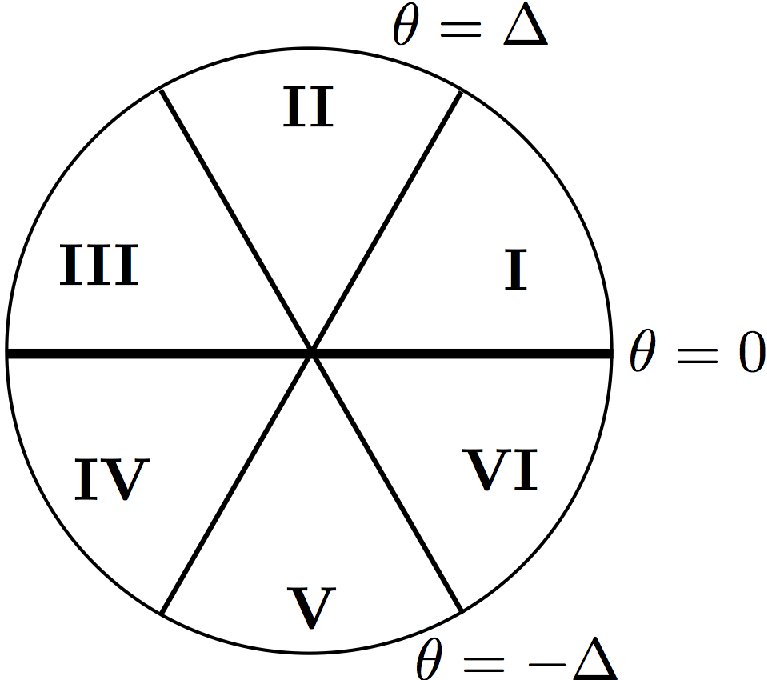
Since two particles of mass are identical, the wave function satisfies or , respectively, for bosons or fermions. In addition, the hyperspherical Hamiltonian is symmetric under and the wave function is either even or odd under this transformation. It is thus sufficient to solve the angular problem only in the domain . Moreover, we will assume that the distinguishable particles are impenetrable. Physically, this is realized by regularizing the inverse square potential (1) with a short-range potential that has a strong repulsive core. Due to the interspecies impenetrability, sectors I and II in Fig. 1 decouple and can be addressed separately. In sector I the hyperangular wave function, , should satisfy the following boundary conditions for [25]
| (7) |
and for
| (8) |
The critical mass ratio is determined by solving Eq. (6) in sector I and is plotted in Fig. 2 (a) and (b) for bosons and fermions, respectively. We found that is an increasing function of the mass ratio for any choice of and boundary conditions. In addition, we find no zero-energy () solution in sector II that satisfies the proper scale-invariant boundary conditions at the interspecies coincidence point. The wave function is thus zero in sector II, i.e., the probability to find the particle of mass in between the two identical particles of mass vanishes.

.
It should be noted that the modified Calogero problem of the type (3) is exactly solvable and scale invariant for the plus-branch under the condition [26, 27, 28]. The Efimov region corresponds to higher values of and, since the problem is not solvable, we solve it numerically. We use the Numerov method [29] on a logarithmic grid (see Ref. [22]). Nevertheless, we also find approximate analytic solutions for this problem in limiting cases discussed below.
For the plus-branch the critical mass ratio diverges at . In fact, for both branches give rise to the Efimov effect for sufficiently large 22 2 This is also true in a three-dimensional version of the problem since in that case the critical value of , where the two-body problem becomes Efimovian, is also . In two dimensions the critical value is exactly zero, so no three-body Efimov effect is possible.. Indeed, for the angle and the hyperangular potential in Eq. (5) reduces to . One can see that the hyperangular problem becomes Efimovian for independent of the quantum statistics of the heavy particles and the branch choice. This means that the spectrum of is unbound from below with deep bound states localized close to . As a result, a finite is necessary to renormalize this potential and bring the ground state energy to zero. Quantitatively, for the plus-branch solution in the vicinity of we obtain [22]
| (9) |
where the upper (lower) sign corresponds to the case of bosons (fermions) and with being the harmonic number.
For the minus-branch the spectrum is Efimovian for any for [22]. The less stringent condition for the Efimov effect in this case can be explained by the fact that the minus-branch two-body interaction nearly binds two particles and is, in this sense, more attractive than the plus-branch interaction with the same . In fact, the hyperangular problem can be solved analytically close to the non-interacting point . In Ref. [22] we show that for the bosonic case
| (10) |
and for fermions
| (11) |
The asymptotes (9), (10), and (11) are plotted in Figs. 2 as dashed lines.
The identified critical mass ratio is calculated using the wave function without nodes inside sector I. As one increases the mass ratio, wave functions with increasing number of nodes will give rise to additional towers of Efimov states.
Now we describe the qualitative nature of the three-body bound state spectrum.The interaction in Eq. (1) must be regularized at short distances, see [22]. As the short-range potential depth changes one can tune between a pure plus-branch () and minus-branch () solutions. The nature of the three-body spectrum will depend on which region in Fig. 2 the system falls into. There are three different regimes:
- •
In the region (i), below the orange curve, there is no Efimov effect for any value of .
- •
In the region (ii), between the orange and blue critical curves, the spectrum behaves similar to the original Efimov problem [1]. By starting from the plus branch solution with and increasing the depth , three-body bound states emerge one-by-one from the three-body continuum as one approaches . At the critical point , where a zero-energy two-body bound state pops up, an infinite tower of Efimov states is formed with the Efimov parameter (encoding the geometric factor for the energy spectrum) which depends on both and . As one further increases the depth , the trimers disappear one-by-one into the particle-dimer continuum.
- •
In the region (iii) the spectrum resembles the one appearing in the three-dimensional Efimov problem of particles with unequal scattering lengths [2, 31, 32]. Now both the plus- and minus-branches support Efimov states characterized by the Efimov parameter and , respectively, where . The energy spectrum contains an infinite number of three-body bound states close to the zero-energy threshold for any value of . The interpolation from the plus- to the minus-branch can be understood as follows: Near the energy spectrum close to the zero-energy threshold is controlled by the parameter. As one approaches the virtual dimer state of size of order is formed. As a result, the trimers with energies below (above) follow the geometric scaling with the Efimov parameter (). At resonance the geometric spectrum with scaling is obtained. When the depth is increased further, a two-body bound state is formed and three-body states with energies below (above) will also follow the geometric scaling with the Efimov parameter () to the point where, when away enough from , the energy spectrum is again completely controlled by the parameter.
Can the Efimov effect found in this paper be discovered experimentally? A promising candidate might be a mixture of dipoles and charges that are confined to one dimension. Indeed, the dipole-charge interaction in three dimensions is given by the scale-invariant anisotropic potential where is the angle between the direction of the dipole moment and the dipole-charge separation vector. Consider now a system of two identical dipoles of mass and dipole moment and a particle of mass and charge confined to a one-dimensional line. Let us also regard the dipoles as dumbbells with fixed dipole moments as illustrated in Fig. 3.

.
This three-body problem is governed by the Hamiltonian
| (12) |
where the Coulomb constant . If we neglect the dipole-dipole term, this Hamiltonian maps on Eq. (3) with
| (13) |
and thus gives rise to the Efimov effect provided and the mass ratio is above the critical value. The presence of the dipole-dipole term introduces a length scale and bound states of this size. In the Efimov regime the length provides the high-energy cutoff for the energy spectrum. This cutoff should not affect the (geometric) energy spectrum close to the zero-energy threshold. However, since our problem is one-dimensional, the dipole-dipole interaction effectively fermionizes the dipoles since their wave function is suppressed at . Thus, the critical mass ratio for the Efimov effect should be read off of Fig. 2 (b) rather than (a) even if the dipoles are identical bosons.
As an example, consider two polar molecules interacting with an electron. From Eq. (13) the dipole moment of the polar molecule should satisfy , where is the charge of the electron and is the Bohr radius. Such a system has a large mass ratio, and, therefore, provided it falls into the region (iii) in Fig. 2 (b), displays Efimov states (without fine-tuning to the minus branch) which can be detected spectroscopically. For a typical mass ratio we find for . Moreover, Efimov states could also be observed if tuning of the dipole moment is possible. In that case, near an electron-dipole resonance, dipolar losses should be enhanced every time a new Efimov state is formed.
A three-dimensional version of the problem may have better chances to be realized experimentally and should also have interesting quantum-chemistry implications. In that case [33, 34, 35]. We consider it as a promising project and leave it for future studies.
Acknowledgements.
We thank S. Endo, O. Kartavtsev, Y. Nishida, S. Tan for useful suggestions. We are grateful to V. Efimov for discussions concerning the qualitative nature of the energy spectrum. This research was partially supported by the NSF through DMR-1001240. SM is grateful for hospitality to Institute for Nuclear Theory in Seattle, where this work was partially done. JPD acknowledges support from the U. S. National Science Foundation. DSP acknowledges support from the IFRAF Institute. The research leading to these results has received funding from the European Research Council under European Community’s Seventh Framework Programme (FR7/2007-2013 Grant Agreement no.341197).References
- [1] V. Efimov, Phys. Lett. B 33, 563 (1970).
- [2] V. Efimov, Nucl. Phys. A 210, 157 (1973).
- [3] E. Nielsen, D. V. Fedorov, A. S. Jensen, and E. Garrido, Phys. Rept. 347 (2001).
- [4] E. Braaten and H. W. Hammer, Phys. Rep. 428, 259 (2006), arXiv:0502080 [nucl-th] .
- [5] D. S. Petrov, Proceedings of the Les Houches Summer Schools, Session 94, edited by C. Salomon, G. V. Shlyapnikov, and L. F. Cugliandolo (Oxford University Press, Oxford, England, 2013), arXiv:1206.5752.
- [6] Y. Wang, J. P. D’Incao, and B. D. Esry, Adv. At. Mol. Opt. Phys. 62, 1 (2013).
- [7] Y. Nishida and S. Tan, Few-Body Syst. 51, 191 (2011), arXiv:1104.2387 .
- [8] Y. Nishida and D. Lee, Phys. Rev. A 86, 032706 (2012).
- [9] Y. Nishida, Y. Kato, and C. D. Batista, Nat. Phys. 9, 93 (2013).
- [10] T. Kraemer, M. Mark, P. Waldburger, J. G. Danzl, C. Chin, B. Engeser, A. D. Lange, K. Pilch, A. Jaakkola, H.-C. Nägerl, and R. Grimm, Nature 440, 315 (2006).
- [11] F. Ferlaino and R. Grimm, Physics (College. Park. Md). 3 (2010).
- [12] B. Huang, L. A. Sidorenkov, R. Grimm, and J. M. Hutson, Phys. Rev. Lett. 112, 190401 (2014).
- [13] R. Pires, J. Ulmanis, M. Repp, A. Arias, E. D. D. Kuhnle, S. Häfner, M. Repp, A. Arias, E. D. D. Kuhnle, and M. Weidemüller, Phys. Rev. Lett. 112, 250404 (2014), arXiv:1403.7246 .
- [14] S.-K. Tung, K. Jiménez-García, J. Johansen, C. V. Parker, and C. Chin, Phys. Rev. Lett. 113, 240402 (2014).
- [15] C. Chin, R. Grimm, P. Julienne, and E. Tiesinga, Rev. Mod. Phys. 82, 1225 (2010).
- [16] M. Kunitski, S. Zeller, J. Voigtsberger, A. Kalinin, L. P. H. Schmidt, M. Schöffler, A. Czasch, W. Schöllkopf, R. E. Grisenti, T. Jahnke, D. Blume, and R. Dörner, Science 348, 551 (2015).
- [17] If three-body discrete scale invariance appears only close to the threshold at zero energy, a short distance structure of the two-body potential does not have to be scale invariant. For example, any short-range potential tuned to a resonance is low-energy scale invariant.
- [18] L. Landau and E. Lifshitz, Quantum Mechanics, Non-Relativistic Theory, Vol. 3 (Pergamon Press, 1965).
- [19] K. M. Case, Phys. Rev. 80, 797 (1950).
- [20] B. Sutherland, J. Math. Phys. 12, 246 (1971).
- [21] D. B. Kaplan, J.-W. Lee, D. T. Son, and M. A. Stephanov, Phys. Rev. D 80, 125005 (2009).
- [22] Supplemental Material contains details on the short-range regularization, Numerov method, analytic calculation near and , and Born-Oppenheimer approximation.
- [23] F. Calogero, J. Math. Phys. 10, 2191 (1969).
- [24] In three dimensions, Guevara et al., Phys. Rev. Lett. 108, 1 (2012) found numerically an infinite number of three-body bound states with the accumulation point at zero energy in a small window of .
- [25] Due to the well-known equivalence of identical spinless fermions and impenetrable bosons in one dimension [M. Girardeau, J. Math. Phys. 1, 516 (1960)], our fermionic results can be directly applied to bosons interacting by a short-range potential. Such interacting bosons can always be considered impenetrable at sufficiently small energies (large distances).
- [26] V. Y. Krivnov and A. A. Ovchinnikov, Theor. Math. Phys. 50, 100 (1982).
- [27] D. Sen, Nucl. Phys. B 479, 554 (1996).
- [28] S. Meljanac, M. Mileković, and A. Samsarov, Phys. Lett. B 573, 202 (2003).
- [29] P. Giannozzi, “Numerical Methods in Quantum Mechanics,” (2014), unpublished.
- [30] This is also true in a three-dimensional version of the problem since in that case the critical value of , where the two-body problem becomes Efimovian, is also . In two dimensions the critical value is exactly zero, so no three-body Efimov effect is possible.
- [31] J. P. D’Incao and B. D. Esry, Phys. Rev. Lett. 103, 083202 (2009).
- [32] Y. Wang, J. Wang, J. P. D’Incao, and C. H. Greene, Phys. Rev. Lett. 109, 243201 (2012).
- [33] K. Connolly and D. J. Griffiths, Am. J. Phys. 75, 524 (2007).
- [34] H. E. Camblong, L. N. Epele, H. Fanchiotti, and C. A. García Canal, Phys. Rev. Lett. 87, 220402 (2001).
- [35] P. R. Giri, K. S. Gupta, S. Meljanac, and A. Samsarov, Phys. Lett. A 372, 2967 (2008).
I Supplemental material: Generalized Efimov effect in one dimension
I.1 Square well regularization and resonance
Consider two particles with the reduced mass interacting in one dimension via the regularized inverse square potenital
| (S1) |
where , . We will also assume , which implies that a wave function should be either even or odd under the reflection . It should be noted that the regularized potential necessarily supports a parity-even ground state with energy . This is in agreement with a general theorem that any attractive well supports at least one bound state in one dimension. Here, however, are interested in the zero energy solution.
For a general solution of the relative Schrödinger equation at zero energy is given by
| (S2) |
On the other hand, for the solution at zero energy is
| (S3) |
By matching the logarithmic derivative at one finds for the reflection odd case
| (S4) |
For the reflection even case one must replace in Eq. (S4). For a generic value of , the plus-branch is dominant for since . Note however that one can fine tune the regularized potential such that the wave function follows the minus-branch for . This happens for resulting in the resonance condition
| (S5) |
By increasing the depth of the short-range potential, the total potential supports more and more bound states. Incidentally, the resonance condition signals the appearance of an additional bound state emerging from the zero-energy threshold.
I.2 Logarithmic grid and Langer substitution
A numerical solution of the Schrödinger equation
| (S6) |
with a potential possessing an inverse square singularity requires a grid which is dense near the singularity allowing to resolve the behavior of the wave function close to it. This can be accomplished by the Langer substitution
| (S7) |
which transforms Eq. (S6) into
| (S8) |
with
| (S9) |
This equation is now solved by the Numerov method on the equidistant -grid with a lower cutoff .
I.3 Analytic calculation near
Slightly above for the plus-branch the critical mass ratio is large () and the angular problem can be attacked analytically. Here we sketch this calculation. First, it is convenient to redefine the angle to be . The angular Schrödinger equation (6) to be solved in sector I takes the form
| (S10) |
where .
In the regime this equation simplifies to
| (S11) |
with a general solution
| (S12) |
where and are associated Legendre functions. The quantum statistics condition (7) imposed at fixes the ratio .
In the regime one can expand the denominators in Eq. (S10) and it transforms to
| (S13) |
with a general solution
| (S14) |
where . The ratio is now determined by applying the plus-branch boundary condition at [equivalent to Eq. (8)].
In the intermediate regime and the wave functions (S12) and (S14) must now be matched. In this region they are given by
| (S15) |
where with a real phase . The phases extracted from the solutions (S12) and (S14) can differ only by the angle , where is an integer. The nodeless wave function is found for . The matching of the phases in the intermediate region with gives rise to Eq. (9).
I.4 Analytic calculation near
Here we show how the mass ratio for the minus-branch can be determined analytically close to the non-interacting point . In this case identical bosons and fermions must be treated differently.
In the case of identical bosons the critical mass ratio vanishes at . We can thus start from the analytical solution of the angular equation (6) at
| (S16) |
with the positive eigenvalue
| (S17) |
Let us now take into account a small deviation of from perturbatively. In order to do this we redefine the angle such that the configurational space is the fixed interval independent of . After this redefinition, Eq. (6) becomes
| (S18) |
where . The linear shift of with respect to is now determined by the first-order perturbation formula
| (S19) |
where is the first derivative of the potential in Eq. (S18) with respect to at and is given by Eq. (S16). We have explicitly
| (S20) |
In fact, the integrals on the right hand side of Eq. (S19) can be calculated for a constant , i.e., setting in Eq. (S16). Then, combining the result with Eq. (S17) we finally obtain
| (S21) |
from which Eq. (10) follows immediately.
I.5 Born-Oppenheimer approximation for minus-branch
Here we study the minus branch in the regime , where the Born-Oppenheimer (BO) approximation can be used and the emergence of the Efimov effect can be intuitively understood. Within this approximation the three-body wave function is factorized
| (S22) |
where the function corresponds to a bound state of the light particle in the combined potential of two heavy centers located at and . This wave function satisfies
| (S23) |
Note that the distance is the only characteristic length scale in Eq. (S23). Therefore, if a bound state exists at some , it also exists at any , and its energy equals , where is a positive dimensionless number which depends on and on the choice of the light-heavy boundary condition.
Next, the Born-Oppenheimer approximation assumes that the light particle adiabatically follows displacements of the heavy ones for which acts as the effective interaction potential. Thus, the Schrödinger equation for the relative motion of the heavy particles reads
| (S24) |
The energy spectrum determines the energy spectrum of the three-body system. The spectrum of Eq. (S24) is Efimovian, , where . For simplicity, we neglected in Eq. (S24) the diagonal correction to the potential which is subleading and does not modify the argument above.
Now we demonstrate that Eq. (S23) actually supports at least one bound state for the minus-branch condition for any . To this end, we consider the minus branch variational wave-function which equals
| (S25) |
for and vanishes for . We find that for any and for a sufficiently small variational parameter
| (S26) |
This can be seen by evaluating analytically the variational energy (S26) and Taylor expanding it around . We thus arrive at the conclusion that for the minus-branch boundary condition the BO approximation demonstrates that the energy spectrum of our three-body system is Efimovian for any in the limit .