Self-Consistent Green’s Function Embedding for Advanced Electronic Structure Methods Based on a Dynamical Mean-Field Concept
Abstract
We present an embedding scheme for periodic systems that facilitates the treatment of the physically important part (here the unit cell) with advanced electronic-structure methods, that are computationally too expensive for periodic systems. The rest of the periodic system is treated with computationally less demanding approaches, e.g., Kohn-Sham density-functional theory, in a self-consistent manner. Our scheme is based on the concept of dynamical mean-field theory (DMFT) formulated in terms of Green’s functions. In contrast to the original DMFT formulation for correlated model Hamiltonians, we here consider the unit cell as local embedded cluster in a first-principles way, that includes all electronic degrees of freedom. Our real-space dynamical mean-field embedding (RDMFE) scheme features two nested Dyson equations, one for the embedded cluster and another for the periodic surrounding. The total energy is computed from the resulting Green’s functions. The performance of our scheme is demonstrated by treating the embedded region with hybrid functionals and many-body perturbation theory in the GW approach for simple bulk systems. The total energy and the density of states converge rapidly with respect to the computational parameters and approach their bulk limit with increasing cluster (i.e., unit cell) size.
Keywords:
Suggested keywordspacs
Valid PACS appear hereI Introduction
Density-functional theory (DFT) has become a widely applied electronic-structure theory method due to the balance between accuracy and computational efficiency of local and semi local approximations such as the local-density (LDA) and generalized gradient approximations (GGA). However, LDA and GGAs suffer from certain intrinsic limitations such as the self-interaction error [1, 2, 3], the absence of the derivative discontinuity in the exchange-correlation potential [4, 5, 6], the lack of long-range van der Waals interactions [7, 8, 9], and the absence of image effects [10, 11, 12]. These shortcomings limit the predictive power of LDA and GGAs, in particular for localised electrons as found in - or -electron systems [13, 14, 15, 16, 17] or for adsorbates and surfaces. [18, 19, 20, 21] Furthermore, DFT is inherently a ground-state method and therefore of limited applicability for excited states and spectra. More advanced electronic-structure methods that overcome one or several of the mentioned shortcomings exist, but they are typically computationally much more demanding and thus limited to small systems sizes or a subset of electronic degrees of freedom. To overcome the efficiency-accuracy conundrum, much effort has been devoted to combine the best of both worlds, that is to merge local and semilocal DFT approximations (DFA) with advanced electronic methods[22, 23, 24, 25, 26, 27, 28, 29, 30, 31, 32, 33, 34, 35].
We here advocate the concept of embedding. In this divide and conquer approach, the full system is divided into two parts: a small embedded region, which is treated with advanced, computationally demanding approaches, and an embedding environment that is treated with computationally more efficient approaches. A schematic illustration of the embedding concept is shown in Fig. 1.

Following this general principle, various embedding schemes have been developed in the past [22, 23, 24, 25, 26, 27, 28, 29, 30, 31, 32, 33, 34, 35, 36]. They differ in scope (i.e., area of application), on how they treat the coupling between the embedded region and the surrounding, and in the approaches used to describe the two regions. In (bio)chemistry, for example, one of the most popular embedding schemes combines quantum mechanics (QM) and classical molecular mechanics (MM). The embedded region is treated quantum mechanically and the surrounding by MM. [23, 24, 25, 26, 27] In surface science, fully quantum mechanical schemes are more prevalent, e.g., for the description of surface adsorbates. They divide space into regions for advanced and less advanced electronic-structure approaches and differ mostly on how these two regions are coupled, e.g. through maximal exchange overlap [28], density embedding [29] or cluster extrapolation [30, 31]. In solid-state physics, dynamical mean-field theory [32, 33, 34] offers a natural embedding framework by mapping an infinite, correlated lattice model into an impurity model [37] immersed into a self-consistently determined mean-field bath. When DFA is chosen as the mean field, DMFT becomes material specific[34, 38, 39]. The embedding is achieved by means of Green’s functions facilitating the calculation of spectra, band structures, but also phase diagrams. Recently, Zgid and Chan [22] proposed to use DMFT as an embedding framework for quantum-chemistry approaches such as the configuration-interaction (CI) method. They since proposed a simplified DMFT scheme based on density-matrix embedding to access static properties (e.g., the ground-state energy and its derivatives)[35]. However, at present all DMFT approaches use a down-folding procedure to a low energy subspace, which is treated on the model-Hamiltonian level.
We here extend the DMFT concept to couple two first-principles regions. Our idea is similar to that of Zgid and Chan[22], but we explore the possibility of using DMFT as a general embedding scheme for advanced first-principles electronic-structure methods. These can be advanced DFT exchange-correlation functionals or excited-state methods based on the approach [40], which are still computationally too expensive for large-scale systems. The difference to previous DMFT schemes is that we treat the unit cell as the local, embedded region, that is coupled to the rest of the periodic system via the DMFT framework. The advantage of our approach is that all electrons in the embedded region are treated on the same quantum mechanical level, which removes the arbitrariness in the definition of the down-folded subspace and does not require any double counting corrections. Furthermore, our approach includes non-local interactions in the embedded region, whose size can be systematically converged to the thermodynamic limit.
We here present the concept of our real-space dynamical mean-field embedding (RDMFE) approach and its implementation in the all-electron Fritz Haber Institute ab initio molecular simulations (FHI-aims) code [41, 42, 43]. We first benchmark it for hybrid density functionals for which we have a periodic reference [44]. Then we apply our scheme to the approach. Due to its intrinsic self-consistency, our RDMFE approach yields a self-consistent solution, which is a much coveted approach for solids right now. While fully self-consistent implementations for molecules are slowly emerging [45, 46, 47, 48, 49, 50], we are only aware of one recent implementation of fully self-consistent for solids [51, 52], which is, however, limited to small unit cells due to its computational expense. An alternative, approximate way to achieve self-consistency within is the so-called quasiparticle self-consistent (QPscGW) scheme, [53, 54] which was recently been widely applied to solids. We here present self-consistent spectra and ground-state energies for simple solids.
The rest of the paper is organized as follows: The detailed formalism of our Green’s-function based embedding scheme is derived in Section II. Section IV presents benchmark results including both total energies and band structures for simple bulk systems. In Section V we contrast our approach with the aforementioned embedding schemes. Section VI concludes the paper.
II Self-Consistent Green’s function Embedding in Real Space
II.1 General concept
In its original formulation, [34] DMFT is a Green’s function method for correlated model Hamiltonians that uses the locality of the electronic interaction to embed a local on-site region of the Hubbard lattice – typically a single - or -level – into a periodic electronic bath defining a self-consistent scheme. Treating the on-site region locally facilitates the use of computationally very demanding and at the same time very accurate methods such as continuous time quantum Monte-Caro [55], direct diagonalization or renormalization group techniques [56]. The localized region is then coupled through a hybridization self-energy to the surrounding electronic bath, which is treated with computationally more efficient methods. In the last few years, DMFT has proven to be very successful in describing the spectral properties of solids with localised - and -states [57, 58, 59, 60]. However, present versions of DMFT also suffer from certain shortcomings. For example, a double counting problem arises when local or semilocal DFA is used to calculate the electronic surrounding, because the DFA contribution of the localised manifold, which would have to be subtracted in order to not count it twice, is not known [61]. Different double counting schemes can give vastly different answers in DFA+DMFT [62, 63]. Last, but not least, the choice of the local manifold can have a considerable impact on the result, in particular when the localised states hybridise with delocalised states in the system [64, 65]. In principle, one could use renormalisation groups to derive the most suitable low energy Hamiltonian for the localised region systematically. However, in practice this is not tractable computationally.
In this work, we use the concept of DMFT and formulate it as a Green’s function embedding scheme for the first-principles Hamiltonian. In contrast to the original DMFT formulation for correlated model Hamiltonians, we consider the unit cell (or any computational supercell that can span the whole space when periodically repeated) as embedded cluster in an first-principles way (see Fig. 2). Our approach therefore includes all electronic degrees of freedom and does not require any downfolding. Our approach also permits the charge flow from one region to the other and therefore naturally incorporates the boundary between the two regions. No special treatment is necessary for atoms on the boundary, nor is it a problem with the boundary cuts covalent bonds.

II.2 Embedding scheme based on DMFT
II.2.1 Green’s function in a non-orthogonal basis set
The embedding framework of DMFT is most conveniently formulated in terms of Green’s functions. In a finite (and generally nonorthogonal) basis set , the Green’s function can be expanded as,
| (1) |
where is the matrix form of the Green’s function. Here we use the Green’s function on the imaginary frequency axis for computational convenience and without loss of generality. For a non-interacting Hamiltonian (e.g., the Kohn-Sham Hamiltonian), the corresponding non-interacting Green’s function in its matrix form satisfies
| (2) |
where is the overlap matrix of the basis functions, and is the chemical potential. Using the Dyson equation that connects the non-interacting Green’s function with the fully interacting one (), we obtain
| (3) |
where is the electronic self-energy. For periodic systems, the Hamiltonian and the Green’s functions are characterized by a Bloch -vector in the first Brillouin zone of reciprocal space. Equation 3 thus becomes
| (4) |
with the lattice Green function . Our implementation is based on the all-electron FHI-aims code package, [41] which uses numerical atom-centered orbitals (NAOs) as its basic functions. The basis functions will thus be NAOs in our work.
II.2.2 The “on-site” Green’s function for a periodic system
The -dependent Green’s function and self-energy in Eq. (4) can be Fourier-transformed to real-space,
where and are Bravais lattice vectors denoting the unit cells in which the basis functions and are located. is the number of -points in the first Brillouin zone (1.BZ). The concept of DMFT is based on the fact that the lattice self-energy becomes local, or -independent, in infinite dimension (). [32] For a crystal with translational symmetry this implies
| (6) |
Thus the self-energy is non-zero only if the two basis functions originate from the same unit cell. We call this the local (loc) or “on-site” self-energy, following the terminology of the model-Hamiltonian studies. In this limit, the whole periodic system can be mapped onto an effective impurity model of a local unit cell dynamically coupled to an effective “external” potential arising from the rest of the crystal.
The first step to establish this mapping is to define the “on-site” Green’s function, i.e., with =. Using the locality of the self-energy and Eq. (4), we obtain the following expression for the onsite Green’s function,
| (7) |
In the DMFT context this equation is also known as the -integrated Dyson equation. So far we have not specified . In our embedding scheme, the environment is treated by KS-DFA in the LDA or the Perdew-Burke-Ernzerhof (PBE)[66] GGA. A natural choice of is thus the KS-Hamiltonian within LDA or GGA, that contains the kinetic-energy operator, the external potential (), the Hartree potential (), and the exchange-correlation (XC) potential ()
| (8) |
Next, we need to define in Eq. (7). If we start from , the “on-site” self-energy becomes the difference between the dynamic, complex many-body exchange-correlation self-energy and the KS XC potential, i.e.,
| (9) |
Using Eqs. (7) and (9), we finally obtain
| (10) |
Our scheme is thus free from any double-counting ambiguities, because the DFA XC-contribution that has to be subtracted is uniquely defined.
II.2.3 Embedded Green’s function
In the DMFT formalism, a periodic system is viewed as a periodically repeated cluster (here the unit or supercell) dynamically embedded into a self-consistently determined environment. The coupling between the embedded subsystem and its surrounding environment is described by a so-called bath Green’s function , connecting the Green’s function of the embedded cluster and the local self-energy via
| (11) |
Here the local self-energy is the same as introduced in Eq. (9). The self-consistency condition of DMFT requires that the Green’s function of the embedded cluster equals the on-site Green’s function as given in Eq. (7),
| (12) |
Alternatively, one can also use a so-called hybridization function to describe the coupling between the embedded cluster and its environment, which provides a more intuitive picture. is closely related to the bath Green’s function ,
| (13) |
In Eq. (13) is the Hamiltonian of the bare cluster describing the non-interacting unit cell i.e., without the contribution and without the presence of the other atoms from neighboring unit cells (see Fig. 2). This corresponds to the “on-site” term of the Hamiltonian of the periodic system, and in practice can be conveniently obtained from the -dependent Hamiltonian,
| (14) |
Using eqs. (11)-(13), we obtain the following expression for the Green’s function of the embedded cluster
| (15) |
Here we have explicitly indicated that the local self-energy is a functional of the embedded Green’s function. Thus eq. (15) has to be solved self-consistently, which corresponds to the inner loop of Fig. 4. The functional dependence of on is given by the actual approximation for the localized region, which will be the topic of next section. However, already here we see that our RDMFE approach lends itself to those advanced electronic-structure methods that can be expressed by (self-consistent) Green’s functions.
Another point we would like to emphasize is the choice of the cluster overlap matrix in eq. (13). We found when updating the chemical potential of the cluster in the inner loop that we needed to define the cluster overlap matrix as (and not simply ) as done by Kotliar et al. [38] to enforce the correct asymptotic behavior of , i.e. .
II.3 The local self-energy
So far we had not specified the approximation for the local self-energy in eq. (15). In our scheme the choice for can be quite flexible. In other words, we could use any approximation that goes beyond LDA and GGAs. However, our framework lends itself to Green’s-function-based approaches. This includes density-matrix and density-based approaches, because both quantities can easily be extracted from the Green’s function. Below we report on two different examples, namely hybrid density functionals that mix a fraction of exact-exchange with GGA semi-local exchange [67, 66, 68] and the approximation. [40] In practice, we could also go beyond , e.g., by including the screened second-order exchange (SOSEX) self-energy that was developed recently. [69]
We here use the PBE hybrid functional family (PBEh) [70], whose most prominent functional is PBE0. [71] We will also use the short-ranged range-separated hybrid functional family by Heyd, Scuseria and Ernzerhof (HSE). [68] In PBEh the local self-energy in eq. (9) is given by
| (16) |
In Eq. (16), is the “on-site” part of the GGA exchange, and is the exact-exchange matrix given by
| (17) |
where are two-electron four-orbital integrals, and is the density matrix of the embedded cluster which can be obtained from the embedded Green’s function
| (18) |
The two-electron Coulomb repulsion integrals are evaluated using the resolution of identity (RI) technique in FHI-aims as documented in Ref. 43. The PBE0 functional is obtained for =0.25. [71]
The extension to an HSE type self-energy is straightforward. In HSE, a range-separation parameter is introduced that cuts off the exact-exchange contribution at long distances. The range is controlled via the screening parameter so that the local exchange self-energy becomes
| (19) |
with SR and LR denoting the short and long-range part, respectively. If we now replace by and introduce the parameter again, the local HSE self-energy assumes the following form
| (20) |
Furthermore, we employ the approximation for the local self-energy. Here, the computation of the self-energy for a given input embedded Green’s function follows the self-consistent implementation for finite systems in FHI-aims. [43, 72] On the imaginary time axis, the self-energy for the embedded cluster is obtained as
| (21) |
Here indices refer to the auxiliary basis set used to expand the screened Coulomb interaction in the RI approach [43, 72]. Furthermore are the 3-index coefficients obtained as,
| (22) |
where
| (23) |
and
| (24) |
with being the auxiliary basis functions. For we thus obtain
| (25) |
where the irreducible polarisability, whose Fourier transform in the time domain is directly determined by the embedded Green’s function
| (26) |
II.4 The self-consistency loops
In our formalism eqs. (15) and (17) or (21) define an additional inner self-consistency loop for the local self-energy as depicted in Fig. 4. Good convergence is achieved by a linear mixing
| (27) |
with a mixing parameter . More advanced mixing schemes could be implemented as well, but we found that linear mixing works well for the examples presented in this work. When the inner-loop reaches convergence we feed the resulting back into the on-site GF and iterate the main-loop further using the same mixing as for the inner-loop.
Finally it is worth mentioning, that the on-site Green’s function as defined in eq. (7) requires that our in the on-site Green’s function in the -th iteration should be . Figure 4 shows a sketch of the embedding scheme as described above. During the self-consistency cycle we compute the particle number , a quantity that is obtained from the embedded Green’s function via
| (28) |
To ensure particle number conservation, we need to update the electron chemical potential every time we receive a converged self-energy from the inner-loop. For the present test cases, we found that the change in the chemical potential is relatively small, as demonstrated in Fig. 3 for bulk silicon (Si). However, we expect it to be more important for metallic systems.


II.5 Total energy calculation
Once self-consistency in the embedding scheme is reached, we can compute the total energy of the entire systems (the embedded cluster plus the environment) using the converged lattice Green function . The actual total-energy expression depends on the chosen methodology used in the embedded region. For hybrid density functionals we have
| (29) |
where
| (30) |
is the matrix form of the kinetic energy operator, the electrostatic (Hartree plus external) energy, and the XC energy. In Eq. (29) is the -dependent global density matrix,
| (31) |
and is the electron density obtained from . We note that Eq. (29) is the exact total-energy expression for the hybrid density functional, and the only approximation is that the density matrix (and hence electron density ) is obtained from the RDMFE scheme and not from a periodic hybrid functional calculation.
However, Eq. (29) cannot be directly applied since evaluating as a functional of the -dependent density matrix requires the computation of the exact-exchange energy for the entire periodic system, which is exactly what we are trying to avoid here. Instead of evaluating in full, we thus only compute the change of with respect to the local or semi-local (LDA or GGA) energy in the embedded region. This is the main approximation of our approach, which is consistent with the spirit of the local self-energy correction in the RDMFE scheme, and is suggested by the near-sightedness of the XC energy of a bulk system (although the exact-exchange energy is probably not the most near-sighted self-energy we could have chosen). [73]
The Hartree energy depends on the electron density in a highly non-local way and it is questionable if a local treatment can be applied to the Hartree energy at all. Therefore, for simplicity, we omit possible changes in the Hartree and the external energy for now, assuming that the electron density given by the local or semi-local approximation is already sufficient.
Finally, we are left with the kinetic energy term which also changes when moving from local or semi-local to hybrid functionals. For consistency, kinetic and XC energy should be taken together. In our scheme, we evaluate the changes of the kinetic and XC energy caused by the local self-energy correction within the embedded region.
Based on the above considerations, we propose the following approximate total-energy expression for embedded hybrid functional calculations
| (32) |
where is the embedded density matrix as defined in Eq. (18), and is the “on-site” density matrix of KS-LDA/GGA calculations. is obtained from the on-site KS density matrix
| (33) |
and is thus restricted to the embedded region.
For we can proceed in an analogous fashion
| (34) |
where
| (35) |
following directly from the Galitskii-Migdal (GM) formula. [74] Similar to the hybrid functional case, we will not take the full dependence in into account. Instead we adopt the same philosophy as before and make a local approximation
| (36) |
where
| (37) |
To summarise this part, in RDMFE the total energy of the entire system can in principle be obtained from the lattice Green’s function. However, in practice, approximations are needed to make the problem tractable. The expressions for hybrid functional and calculations proposed above are consistent with the local nature of the self-energy approximation in RDMFE, but their performance needs to be checked in practical calculations. Future work needs to revisit total energy calculations in RDMFE.
III Computational details
We used tight FHI-aims integration grids for all our RDMFE calculations. For the embedded PBEh and HSE self-energy we used the tier 1 basis set. Figure 5 shows the embedded PBEh total and cohesive energies with increasing basis set size. The lattice Green’s functions were represented on a logarithmic frequency grid with 40 points. The total energy calculations for 2 and 8 atom silicon unit cells and the density of states (DOS) calculations for 8 and 16 atom unit cells were performed on a k-point grid, which we increased to for DOS calculations in the 2 atom unit cell. GW calculations were performed in a tier 3 basis set with 40 frequency/time points in the inner loop and the same number of k-points as for PBEh. The linear mixing parameter was fixed to , which gave reasonably fast convergence. The periodic PBE and PBE0 reference calculations were performed using the tier 1 basis set and a k-mesh.
 |
 |
Densities of states are obtained in two different ways. In PBEh and HSE we obtain a self-energy that defines a converged k-dependent embedded Hamiltonian via the converged lattice Green’s function once the self-consistency cycle is converged. For the PBEh self-energy we can directly diagonalize the embedded Hamiltonian at each k-point, which yields k-dependent eigenvalues and eigenstates. The resulting density of states (DOS) is , where labels the eigenstates of . To make the comparison to experiment easier, we introduce a Gaussian broadening
| (38) |
to obtain the DOS . In this work we use a Gaussian broadening of eV.
For the GW self-energy, the spectrum at each k-point is directly given by the Green’s function as
| (39) |
To determine on the real-frequency axis, we analytically continue the self-energy from the imaginary to the real axis. In practice, we fit a two-pole model, that has proven to work very well for the systems we tested, to each matrix element of the self-energy[75, 43]
| (40) |
where and are complex fitting parameters. We then evaluate eq. (40) for real frequencies and solve Dyson’s equation for . The spectral function subsequently follows from a k-summation , which we convolute with Gaussians as
| (41) |
with a broadening that we choose to be eV to obtain a DOS that we can compare with experiment.
IV Results
Having introduced the concept of RDMFE and our implementation in the previous sections, we now turn to benchmark calculations for hybrid functionals, for which we have an independent, periodic reference in FHI-aims [44]. Then we present self-consistent calculations for which such a periodic reference does not yet exist in FHI-aims. We choose bulk Si as test system since it is a reliable and well studied reference case.
IV.1 Density of states and band structures
We begin our benchmark tests by calculating the DOS at each iteration to investigate its evolution with each embedding cycle. Figure 6 shows the DOS at different iterations of the outer loop for a 2 atom unit cell of silicon. We observe that the largest change occurs at the first iteration when moving from PBE to our embedded PBE0 DOS. For subsequent iterations the DOS changes are much smaller.


 |
 |
When comparing the converged, embedded DOS for the 2 atom unit cell with the periodic PBE and PBE0 DOS shown in Fig. 7, we observe that the band width and band gap are larger than in PBE and are closer to the PBE0 reference. When increasing the unit cell size to 8 and 16 atoms (see Fig. 8) the difference between the embedded DOS and the periodic PBE0 DOS reduces systematically. The resulting RDMFE band gaps for different unit cell sizes are compared with the PBE and the PBE0 values in Tab. 1. With increasing unit cell size, the band gap increases and approaches the PBE0 value.
| RDMFE@PBE0 | ||||||
| PBE | PBE0 | 2 atoms | 8 atoms | 16 atoms | experiment (at 300K)[76] | |
| band gap [eV] | 0.68 | 1.85 | 1.2 | 1.257 | 1.569 | 1.12 |
Next, we consider the band structure for the 2 atom unit cell shown in the upper panel of Fig. 9. We see the same trend as for the DOS: the band gap and the band width approach PBE0 and so do the bands in general. However, at some high symmetry points the degeneracy of certain bands is lifted. The origin of this degeneracy lifting is the break of the crystal symmetry that we introduce with the local self-energy. It is a well known artefact and has been discussed extensively in the context of cellular and cluster DMFT [77, 78]. The local self-energy simply does not “know” about the symmetry of the crystal and can therefore not enforce it. The solution to the problem is then obvious: the approximation of the locality of the self-energy needs to be improved. If the self-energy would extend over a larger region (i.e. supercell) it would acquire more information about the crystal symmetry. Then the degeneracy splitting should reduce. In the two lower panels of Fig. 9, we present an unfolded band structure [79] for the 16 and 32 atom unit cells. We indeed observe a reduction in the splitting for both the 16 and 32 atom unit cells. However, while the degeneracy is fully restored for some high symmetry points, it is still broken for others such as the X and Z points.
 |
 |
 |
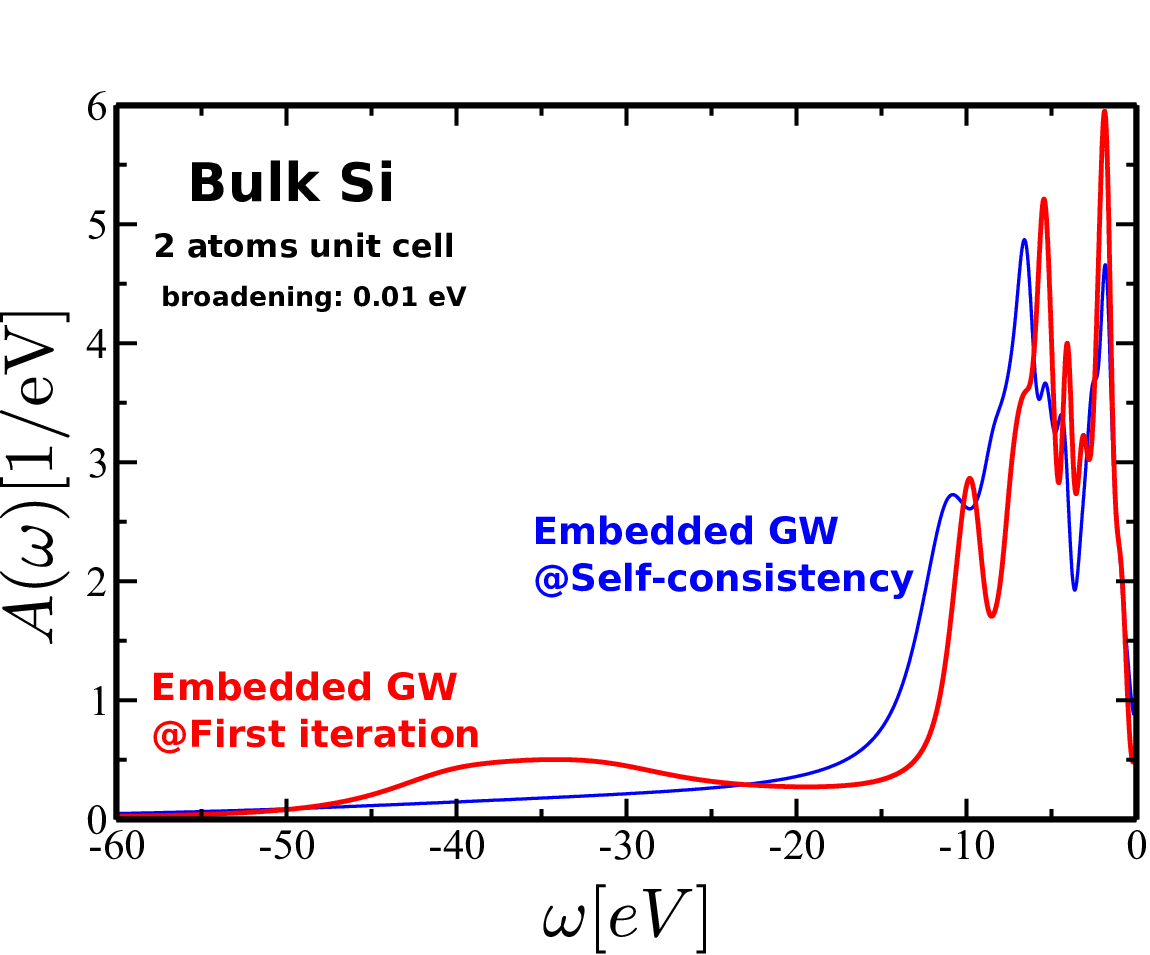
We will now turn to the spectra. The total spectral function for bulk Si with 2 atoms in the unit cell at the 1st iteration is shown in Fig. 10. Since Dyson’s equation has been solved once, this spectrum is not equivalent to perturbative spectra and we would expect to see plasmon satellites. The spectrum shows a broad peak between -40 and -30 eV, which has been identified as plasmon satellite. [80, 81] Such satellites are completely absent in KS band structures or in , because only corrects the KS states and does not yield new states. The energy range of the RDMFE satellite agrees well with previous periodic calculations [80, 81] and demonstrates that our dynamic, local RDMFE framework can capture non-local phenomena such as plasmon satellites. For scGW the converged DOS is also shown in Fig. 10. As demonstrated by Holm and von Barth [82] for the electron gas, full self-consistency in and leads to a deterioration in the GW spectral function due to the neglect of vertex corrections. Thus, the fact, that the plasmon satellite disappears at self-consistency is not surprising.
We obtain a band gap of 0.9 eV for the two atom unit cell, which is close to the experimental value of 1.12 eV [83]. This comparison together with the one between the indirect band gap from our calculation and experiment[76] are presented in Tab. 2.
| band gap | RDMFE@scGW | periodic scGW[51] | scGW[54] | experiment (at 300K) |
|---|---|---|---|---|
| direct () [eV] | 3.7 | — | 3.47 | 3.4 [76] |
| indirect () [eV] | 0.9 | 1.55 | 1.25 | 1.12 [83] |
IV.2 Embedded total energies:
For sc we currently do not have a periodic reference to compare to, as alluded to before. We can, however, construct another test case and benchmark against our sc implementation for finite systems[47, 48], where the total energy was computed from the Galitskii-Migdal formula [74]. We achieve this by considering the molecular limit of a unit cell, i.e., the limit of an isolated unit cell with a lattice constant of 20 Å. The benchmark results for He, H2 and Na2 are presented in Tab. 3, which shows the XC components that enter the total energy as given by Eq. (37). is the molecular sc XC self-energy and the corresponding Green’s function at convergence. is local XC self-energy and the embedded Green’s function both obtained at convergence of the RDMFE cycle. Table 3 illustrates that the components entering the embedded total energy agree almost to the meV level with the corresponding components from the finite systems scGW calculation, which demonstrates the reliability and robustness of our implementation.
| Term | He | H2 | Na2 |
|---|---|---|---|
| -27.173906 | -17.503642 | -760.630196 | |
| -27.181325 | -17.505250 | -760.632183 | |
| -1.744578 | -2.3053908 | -2.457104 | |
| -1.737910 | -2.304200 | -2.455707 |
We then investigated the convergence of the total energy with respect to the increase of the unit cell size for RDMFE PBE0 and scGW. For embedded PBE0, we performed calculations for bulk Si up to 32 atoms in the unit cell, whereas for GW we considered bulk He in the fcc structure up to 64 atom unit cells. To reach larger systems, a full parallelization of our implementation would be required. The upper panel of Fig. 11 shows the comparison of our embedded PBE0 cohesive energy with the periodic PBE and the periodic PBE0 energy. We also include a third reference in which we added the kinetic and XC energy of a PBE0 calculation to the PBE energy, which most closely resembles our RDMFE approximation. We see that with increasing unit cell size the embedded cohesive energy approaches the periodic PBE0 value, but then dips below. This is not surprising since our embedded cohesive energy does not account for changes in the electrostatic energy. Instead, the RDMFE curve approaches the PBE0 reference value from which the electrostatic change has been removed. However, the convergence to the periodic limit is relatively slow. This can be related to the long range nature of the HF exact-exchange as we will show later on using a range separated self-energy (see the discussion of Fig. 12). For the GW self-energy, however, the total energy seems to converge much faster and only changes in a very small range. This is shown in the lower panel of Fig. 11.
 |
 |
To better visualise the interplay between locality and unit cell size in our scheme we also present results of the HSE range-separated exact-exchange self-energy. We vary the range separation parameter to model different degrees of locality, but keep the percentage of exact exchanged fixed. We then translate the range separation parameter into a radius in real-space using the relation and determine the number of atoms that fit inside. We have considered range-separation parameters that correspond to spheres enclosing 2, 4, 8 and 16-atom unit cells. For each , the resulting embedded total energy is plotted in Fig. 12 as a function of the size of the unit cell (upper panel). The lower panel shows the volume of the surrounding sphere for the different parameters and for the different unit cell sizes. We indeed observe that the total energy converges faster with unit cell size, the shorter the range of the non-locality in the HSE self-energy. This proofs that RDMFE becomes a viable option for self-energies, whose range only encompasses a few nearest atoms. In that sense, PBE0 had been the toughest test, because its range is infinite.
 |
 |
Finally, we briefly address cohesive properties. In Fig. 13 we show the total energy of bulk Si as a function of the lattice constant for RDMFE@PBE0, scGW and for periodic PBE0. For RDMFE@PBE0 (upper panel) our calculations for a 2 atom unit cell already give a minimum that is below the PBE one and very close to the experimental value of 5.43Å[84] (see Tab. 4). However, for an 8 atom unit cell the lattice constant reduces slightly. For RDMFE@, the minimum for the 2 atom unit cell (lower panel) also lies below the PBE value and already agrees fortuitously well with the experimental value. Our RDMFE@ lattice constant is slightly larger than that reported by a recent periodic self-consistent GW calculation[51]. We also performed a Birch-Murnaghan [85] fit of the total energy curves to extract the bulk moduli for RDMFE@PBE0 and RDMFE@. The resulting values are reported in Tab. 4.
| RDMFE@PBE0 | periodic PBE0 | RDMFE@scGW | periodic scGW[52] | experiment | ||
|---|---|---|---|---|---|---|
| unit cell size | 2 atoms | 8 atoms | 2 atoms | 2 atoms | — | — |
| lattice constant [Å] | 5.45 | 5.4 | 5.43 | 5.43 | 5.39 | 5.43[84] |
| bulk modulus [GPa] | 95.14 | 129.07 | 84 | 80.37 | 100.7 | 99[86] |
 |
 |
V Discussion
We have presented an embedding scheme for periodic systems that builds on DMFT. In our approach, the electron interacting across periodically repeated unit cells is mapped onto an on-site problem, in which the electrons only interact directly in one unit cell, but are dynamically coupled to a periodic bath of electrons. The coupling between the embedded system and the surrounding is constructed naturally by means of Green’s functions. Due to its dynamic nature the bath can exchange electrons with the embedded region. Our embedding scheme is most suitable for systems with periodic boundary conditions, as the translational symmetry is automatically preserved. Furthermore, we transfer the non-locality of a self-energy into a frequency dependence, a concept that has previously been explored by Gatti et al. [87] and in the spectral density-functional theory of Kotliar et al. [88] We note that the only approximation introduced in our scheme is that the non-local XC coupling between neighboring unit cells (or computational supercells) is included only at the KS GGA level, and neglected in the more advanced (here hybrid functional or ) treatment. In other words, the self-energy correction to the GGA XC potential is -independent, an intrinsic feature of DMFT.
We now compare our scheme to other embedding schemes. For the hybrid QM:MM approach a clear separation between the embedded region and the surrounding and the treatment of the boundary atoms is not always obvious[89, 26]. For systems, in which classical electrostatics dominate such as ionic or molecular solids, the separation between ions and molecules is natural. However, for covalently bonded systems it becomes more difficult to define the QM:MM partitioning. Thus, typically covalent bonds are cut at the QM:MM boundary, which produces dangling bonds that need to be saturated. A multitude of models with different levels of accuracies have been developed to tackle these issues. One example is the ChemShell framework [90, 91] that supports Hartree-Fock and hybrid functionals in the embedded region and that has recently been coupled to FHI-aims [36].
Another popular approach is ”Our own N-layer integrated molecular orbital molecular mechanics” (ONIOM) by Morokuma and coworkers. [25, 92] ONIOM is a so-called extrapolative (or subtractive) scheme in which the total energy of the whole system is given by
| (42) |
where the RL refers to the real (or full) system at the lower level, ML refers to the model (or embedded) system at the lower level and MH labels the model system for the higher level theory. In constrat to the additive QM:MM scheme, ONIOM does not need an additional coupling Hamiltonian to describe the QM/MM interation. When a QM/MM boundary cuts through a covalent bond, link atoms (mostly hydrogen atoms) are added to cap the unsaturated QM boundary for the model calculations. Even if it is common to use MM methods for describing the surroundings, the ONIOM scheme was recently extended to deal with two-layer two-QM embedding, ONIOM(QM1:QM2), where HF was used for the surroudings and the embedded model region is described by MP2 or B3LYP. The QM1/QM2 interactions, including electrostatic interaction, mutual polarization, and charge transfer, are described at the lower QM level.
Our RDMFE scheme is distinctly different from the ONIOM(QM1:QM2) approach. First, the RDMFE scheme is formulated in terms of Green’s functions, whereas ONIOM is based on a partition of total energies. As such, spectral properties come out naturally from RDMFE, while the evaluation of total energies is more involved, as discussed in Sec. II.5. The opposite is true for the ONIOM(QM1:QM2) scheme. Second, within RDMFE, the effect of the environment is encoded in the bath Green’s function that describes an electron reservoir with which the embedded cluster can exchange electrons freely. In other words, the electronic states in the embedded system are not forced to localize within the cluster, but are allowed to delocalize into the surrounding system. Thus, dangling bonds pose no conceptual problem and boundary effects are not significant since they diminish quickly as the size of the cluster increases. In contrast, in ONIOM(QM1:QM2), like in most other embedding schemes in computational chemistry, link atoms are needed to saturate the dangling bonds when chemical bonds are broken. Therefore ONIOM(QM1:QM2) is most appropriate for describing systems with localized electrons, whereas RDMFE has no problem in dealing with delocalized electrons, especially metallic systems. Third, RDMFE, as is formulated right now, is only applicable to periodic systems that are relevant to solid state physics, while ONIOM(QM1:QM2) is most suitable for describing molecules and clusters that are of interest to chemical and biological applications.
Addressing the problem of CO adsorption on Cu(111) [18], Hu, Reuter and Scheffler [30, 89] developed a cluster extrapolation scheme that is based on performing a cheap (LDA/GGA) calculation for the periodic system then correcting the resulting total energy by , where and are the cluster XC-energy parts of a cluster calculation with the cheaper (LDA/GGA) and the ”better” theory respectively while the cluster itself has been cut out from the periodic system. Increasing the cluster size, they could then show that the correction converges for relatively small cluster sizes (16 atoms) and thus much faster than alone. This cluster extrapolation concept is similar to that of ONIOM(QM1:QM2) described above, but link atoms were not used for the cluster calculations.
Whitten and coworkers also approached molecular adsorbates on metal surfaces.[28] They developed an embedding scheme that builds on identifying a localized subspace that has maximal exchange overlap with the valence orbitals of the atoms within and bordering the adsorbate. The localized subspace is then solved using the CI method, for a fixed Coulomb and exchange potential constructed from the localized orbitals. However, the approach mimics the real periodic system using a large cluster of atoms, which fails in describing the system accurately. Additionally, no systematic cluster extrapolation has been studied. In a similar spirit, Huang and Carter developed a density-functional-based embedding scheme. [29] The scheme relies on the fact that the density is additive, i.e., that the total electron density can be partitioned into the density of the embedded region and the density of the embedding surrounding. Proceeding as such, allows the definition of an embedding density-potential, that is a functional of the total and the embedded density. Adding this potential to the embedded Hamiltonian and solving the resulting KS Schrödinger equation self-consistently leads to the desired embedded density. For the embedded region, correlated wave function methods are typically used, while for the embedding potential the optimized effective potential method or kinetic energy density functionals are employed. Moreover, due to the static nature of the embedding potential no dynamical methods can be used to describe the embedded region, which limits the applicability to ground state properties.
For point defects in semiconductors, Scheffler et al. [26] devised a self-consistent Green’s function method to compute the change in density induced by the presence of the defect. They considered this change as being a perturbation to the perfect crystal and solved the resulting Dyson equation self-consistently. Using the fact that defects are well localized in real space, they correct the Hellmann-Feynman force of the perfect crystal – calculated with force fields – by a contribution containing the change in density due to the defect – calculated with KS-DFA. They showed that the resulting Hellmann-Feynman force is comparable in accuracy to a full DFA calculation.
Finally, it is also worth mentioning, that we perform fully self-consistent GW calculations [43, 72] in our scheme, which is conceptually different from the so called quasiparticle self-consistent GW concept[53, 54] (QPscGW). In QPscGW a series of calculations is performed. In each iteration the “best” is determined that most closely resembles the Green’s function of the current cycle. In practice a static, non-local potential is constructed that approximates the self-energy. This non-local potential defines a new non-interaction Hamiltonian that produces a new input Green’s function . Since the QPscGW concept also requires the calculation of the full non-local self-energy our expectation is that it will be easier to go beyond in our RDMFE framework.
VI Conclusions
We have presented an embedding scheme for periodic systems based on Green’s functions in the DMFT framework, which maps an infinite periodic system to a single-site (single unit cell) problem coupled to an electronic bath that needs to be determined self-consistently. Our RDMFE Green’s function mapping allows a natural definition of the embedded region and defines a self-consistency loop which, at convergence, yields self-consistent Green’s functions. The coupling to the surrounding is of dynamical nature enabling electron exchange between the embedded region and the surrounding. We showed that our scheme produces densities of states and total energies that converge well with increasing size of the embedded region. We also demonstrated, that the main features of the “better” theory are rapidly captured within our scheme; for example the plasmon satellite already appears in RDMFE@ calculations for 2 atoms in the Si unit cell. RDMFE is therefore a promising embedding scheme, that has the potential to make sophisticated and computationally expensive first-principles theories available for periodic systems.
References
- [1] J. Perdew and A. Zunger, Phys. Rev. B 23, 5048 (1981).
- [2] J. P. Perdew, R. G. Parr, M. Levy, and J. L. Balduz, Phys. Rev. Lett. 49, 1691 (1982).
- [3] P. Mori-Sánchez, A. J. Cohen, and W. Yang, The Journal of Chemical Physics 125, 201102 (2006).
- [4] J. Perdew and M. Levy, Phys. Rev. Lett. 51, 1884 (1983).
- [5] L. Sham and M. Schlüter, Phys. Rev. Lett. 51, 1888 (1983).
- [6] P. Mori-Sánchez, A. J. Cohen, and W. Yang, Phys. Rev. Lett. 100, 146401 (2008).
- [7] O. Gunnarsson and B. I. Lundqvist, Phys. Rev. B 13, 4274 (1976).
- [8] J. F. Dobson and J. Wang, Phys. Rev. Lett 82, 2123 (1999).
- [9] A. Tkatchenko and M. Scheffler, Phys. Rev. Lett. 102, 073005 (2009).
- [10] I. D. White, R. W. Godby, M. M. Rieger, and R. J. Needs, Phys. Rev. Lett. 80, 4265 (1997).
- [11] K. S. Thygesen and A. Rubio, Phys. Rev. Lett. 102, 046802 (2009).
- [12] C. Freysoldt, P. Rinke, and M. Scheffler, Phys. Rev. Lett. 103, 056803 (2009).
- [13] T. C. Leung, X. W. Wang, and B. N. Harmon, Phys. Rev. B 37, 384 (1988).
- [14] J. Zaanen, O. Jepsen, O. Gunnarsson, A. Paxton, O. Andersen, and A. Svane, Physica C: Superconductivity 153–155, Part 3, 1636 (1988), proceedings of the International Conference on High Temperature Superconductors and Materials and Mechanisms of Superconductivity Part {II}.
- [15] W. E. Pickett, Rev. Mod. Phys. 61, 433 (1989).
- [16] L. F. Mattheiss, Phys. Rev. B 5, 290 (1972a).
- [17] L. F. Mattheiss, Phys. Rev. B 5, 306 (1972b).
- [18] P. J. Feibelman, B. Hammer, J. K. Nørskov, F. Wagner, M. Scheffler, R. Stumpf, R. Watwe, and J. Dumestic, J. Phys. Chem. B 105, 4018 (2001).
- [19] I. Mehdaoui and T. Klüner, The Journal of Physical Chemistry A 111, 13233 (2007).
- [20] I. Mehdaoui and T. Klüner, Phys. Rev. Lett. 98, 037601 (2007).
- [21] I. Mehdaoui and T. Klüner, Phys. Chem. Chem. Phys. 10, 4559 (2008).
- [22] D. Zgid and G. K.-L. Chan, J. Chem. Phys. 134, 094115 (2011).
- [23] U. C. Singh and P. A. Kollman, J. Comp. Chem. 7, 718 (1986).
- [24] M. J. Field, P. A. Bash, and M. Karplus, J. Comp. Chem. 11, 700 (1990).
- [25] F. Maseras and K. Morokuma, J. Comp. Chem. 16, 1170 (1995).
- [26] M. Scheffler, J. P. Vigneron, and G. B. Bachelet, Phys. Rev. B 31, 6541 (1985).
- [27] J. Bormet, J. Neugebauer, and M. Scheffler, Phys. Rev. B 49, 17242 (1994).
- [28] J. L. Whitten and T. A. Pakkanen, Rev. Phys. B 21, 10 (1980).
- [29] C. Huang and E. A. Carter, J. Chem. Phys. 135, 194104 (2011).
- [30] Q.-M. Hu, K. Reuter, and M. Scheffler, Phys. Rev. Lett 98, 176103 (2007a).
- [31] X. Ren, P. Rinke, and M. Scheffler, Phys. Rev. B 80, 045402 (2009).
- [32] W. Metzner and D. Vollhardt, Phys. Rev. Lett. 62, 324 (1989).
- [33] A. Georges and G. Kotliar, Rev. Phys. B 45, 6479 (1992).
- [34] W. Metzner and D. Vollhardt, Rev. Mod. Phys. 68, 13 (1996).
- [35] G. Knizia and G. K.-L. Chan, Phys. Rev. Lett. 109, 186404 (2012).
- [36] D. Berger, A. J. Logsdail, H. Oberhofer, M. R. Farrow, C. R. A. Catlow, P. Sherwood, A. A. Sokol, V. Blum, and K. Reuter, The Journal of Chemical Physics 141, 024105 (2014).
- [37] P. W. Anderson, Rev. Phys. B 124, 41 (1961).
- [38] G. Kotliar, S. Savrasov, K. Haule, V. Oudovenko, O. Parcollet, and C. Marianetti, Rev. Mod. Phys. 78, 865 (2006).
- [39] K. Held, Adv. Phys. 56, 829 (2007).
- [40] L. Hedin, Phys. Rev. 139, A796 (1965).
- [41] V. Blum, F. Hanke, R. Gehrke, P. Havu, V. Havu, X. Ren, K. Reuter, and M. Scheffler, Comp. Phys. Comm. 180, 2175 (2009).
- [42] V. Havu, V. Blum, P. Havu, and M. Scheffler, J. Comp. Phys. 228, 8367 (2009).
- [43] X. Ren, P. Rinke, V. Blum, J. Wieferink, A. Tkatchenko, A. Sanfilippo, K. Reuter, and M. Scheffler, New J. Phys. 14, 053020 (2012).
- [44] S. Levchenko, X. Ren, J. Wieferink, P. Rinke, V. Blum, M. Scheffler, and R. Johanni, Comp. Phys. Comm. (2015).
- [45] A. Stan, N. E. Dahlen, and R. van Leeuwen, Europhys. Lett. 76, 298 (2006).
- [46] C. Rostgaard, K. W. Jacobsen, and K. S. Thygesen, Phys. Rev. B 81 (2010).
- [47] F. Caruso, P. Rinke, X. Ren, M. Scheffler, and A. Rubio, Phys. Rev. B 86, 081102(R) (2012).
- [48] F. Caruso, P. Rinke, X. Ren, A. Rubio, and M. Scheffler, Phys. Rev. B 88, 075105 (2013a).
- [49] F. Caruso, D. R. Rohr, M. Hellgren, X. Ren, P. Rinke, A. Rubio, and M. Scheffler, Phys. Rev. Lett. 110, 146403 (2013b).
- [50] P. Koval, D. Foerster, and D. Sánchez-Portal, Phys. Rev. B 89, 155417 (2014).
- [51] A. Kutepov, S. Y. Savrasov, and G. Kotliar, Phys. Rev. B 80, 041103 (2009).
- [52] A. Kutepov, K. Haule, S. Y. Savrasov, and G. Kotliar, Phys. Rev. B 85, 155129 (2012).
- [53] M. van Schilfgaarde, T. Kotani, and S. Faleev, Phys. Rev. Lett. 96, 226402 (2006).
- [54] T. Kotani, M. van Schilfgaarde, and S. V. Faleev, Phys. Rev. B 76, 165106 (2007).
- [55] P. Werner, A. Comanac, L. de’ Medici, M. Troyer, and A. J. Millis, Phys. Rev. Lett. 97, 076405 (2006).
- [56] D. Zgid, E. Gull, and G. K.-L. Chan, Phys. Rev. B 86, 165128 (2012).
- [57] Savrasov S. Y. and Kotliar G. and Abrahams E., Nature 410, 793 (2001), 10.1038/35071035.
- [58] K. Held, A. K. McMahan, and R. T. Scalettar, Phys. Rev. Lett. 87, 276404 (2001).
- [59] B. Amadon, S. Biermann, A. Georges, and F. Aryasetiawan, Phys. Rev. Lett. 96, 066402 (2006).
- [60] J. M. Tomczak, F. Aryasetiawan, and S. Biermann, Phys. Rev. B 78, 115103 (2008).
- [61] M. Karolak, G. Ulm, T. Wehling, V. Mazurenko, A. Poteryaev, and A. Lichtenstein, Journal of Electron Spectroscopy and Related Phenomena 181, 11 (2010), proceedings of International Workshop on Strong Correlations and Angle-Resolved Photoemission Spectroscopy 2009.
- [62] A. I. Lichtenstein and M. I. Katsnelson, Phys. Rev. B 57, 6884 (1998).
- [63] V. I. Anisimov, A. I. Poteryaev, M. A. Korotin, A. O. Anokhin, and G. Kotliar, J. Phys.: Condens. Matter 9, 7359 (1997).
- [64] L. Vaugier, H. Jiang, and S. Biermann, Phys. Rev. B 86, 165105 (2012).
- [65] F. Nilsson, R. Sakuma, and F. Aryasetiawan, Phys. Rev. B 88, 125123 (2013).
- [66] J. P. Perdew, K. Burke, and M. Ernzerhof, Phys. Rev. Lett 77, 3865 (1996).
- [67] A. D. Becke, J. Chem. Phys 98, 5648 (1993).
- [68] J. Heyd, G. E. Scuseria, and M. Ernzerhof, J. Chem. Phys. 118, 8207 (2003).
- [69] X. Ren, N. Marom, F. Caruso, P. Rinke, and M. Scheffler, Submitted.
- [70] M. Ernzerhof and G. E. Scuseria, The Journal of Chemical Physics 110, 5029 (1999).
- [71] C. Adamo and V. Barone, The Journal of Chemical Physics 110, 6158 (1999).
- [72] F. Caruso, P. Rinke, X. Ren, M. Scheffler, and A. Rubio, Phys. Rev. B 88, 075105 (2013c).
- [73] W. Kohn, Phys. Rev. Lett. 76, 3168 (1996).
- [74] V. M. Galitskii and A. B. Migdal, Sov. Phys.-JETP 7, 96 (1958).
- [75] H. N. Rojas, R. W. Godby, and R. J. Needs, Phys. Rev. Lett. 74, 1827 (1995).
- [76] Ioffedatabase, .
- [77] G. Biroli, O. Parcollet, and G. Kotliar, Phys. Rev. B 69, 205108 (2004).
- [78] A. I. Lichtenstein and M. I. Katsnelson, Phys. Rev. B 62, 9283(R) (2000).
- [79] Unit cells larger than the primitive unit cell give rise to a folded band structure. To cast the band structure back onto the Brillouin zone of the 2 atom unit cell we use the unfolding approach of L. Nemec.
- [80] M. Guzzo, G. Lani, F. Sottile, P. Romaniello, M. Gatti, J. J. Kas, J. J. Rehr, M. G. Silly, F. Sirotti, and L. Reining, Phys. Rev. Lett. 107, 166401 (2011).
- [81] J. Lischner, D. Vigil-Fowler, and S. G. Louie, Phys. Rev. Lett. 110, 146801 (2013).
- [82] B. Holm and U. von Barth, Phys. Rev. B 57, 2108 (1998).
- [83] S. O. Kasapa and P. Capper, Springer , 54,327 (2006).
- [84] T. Hom, W. Kiszenik, and B. Post, Journal of Applied Crystallography 8, 457 (1975).
- [85] F. Birch, Phys. Rev. 71, 809 (1947).
- [86] C. O. Rodriguez, V. A. Kuz, E. L. Peltzer y Blanca, and O. M. Cappannini, Phys. Rev. B 31, 5327 (1985).
- [87] M. Gatti, V. Olevano, L. Reining, and I. V. Tokatly, Phys. Rev. Lett. 99, 057401 (2007).
- [88] S. Y. Savrasov and G. Kotliar, Phys. Rev. B 69, 245101 (2004).
- [89] Q.-M. Hu, K. Reuter, and M. Scheffler, Phys. Rev. Lett. 99, 169903 (2007b).
- [90] P. Sherwood, A. H. de Vries, M. F. Guest, G. Schreckenbach, C. A. Catlow, S. A. French, A. A. Sokol, S. T. Bromley, W. Thiel, A. J. Turner, S. Billeter, F. Terstegen, S. Thiel, J. Kendrick, S. C. Rogers, J. Casci, M. Watson, F. King, E. Karlsen, M. Sjøvoll, A. Fahmi, A. Schäfer, and C. Lennartz, Journal of Molecular Structure: {THEOCHEM} 632, 1 (2003).
- [91] A. A. Sokol, S. T. Bromley, S. A. French, C. R. A. Catlow, and P. Sherwood, International Journal of Quantum Chemistry 99, 695 (2004).
- [92] L. W. Chung, H. Hirao, X. Li, and K. Morokuma, WIREs Comput Mol Sci 2, 327 (2012).