Continuum Nanofluidics
Abstract
This paper introduces the fundamental continuum theory governing momentum transport in isotropic nanofluidic flows. The theory is an extension to the classical Navier-Stokes equation, which includes coupling between translational and rotational degrees of freedom, as well as non-local response functions that incorporates spatial correlations. The continuum theory is compared with molecular dynamics simulation data for both relaxation processes and fluid flows showing excellent agreement on the nanometer length scale. We also present practical tools to estimate when the extended theory should be used. It is shown that in the wall-fluid region the fluid molecules align with the wall and in this region the isotropic model may fail and a full anisotropic description is necessary in order to describe this region.
I Introduction
Nanoscale devices can now be fabricated with channels where the smallest dimension is just a few nanometers [1], and the development of nanofluidic theory [2, 3, 1] is more relevant than ever. Consider the following example. Perrson et al. [4] used a series of rectangular nanochannels with widths ranging from 14 to 300 nm to connect two micro-scale chambers. By means of capillary filling, fluid from one chamber fills up the channels and thus connects the two chambers. The filling rate can be measured for different channel widths and for both milli-Q water (filtrated de-ionized water) and an electrolyte solution of sodium chloride. The rate did not follow the Washburn equation for channel widths smaller than 100 nm. The Washburn equation is based on the classical continuum picture [3] using Poiseuille law of fluid motion which includes the Newtonian (or macroscopic) shear viscosity. For widths larger than 100 nm the Washburn equation correctly predicts the filling rate. This is in accordance with the common understanding that the discrete nature of the fluid at small scales destroys the continuum picture [2, 6]. In fact, many researchers categorize continuum physics as physics on the macroscopic scale, see for example Ref. 7. Several questions immediately arise: When exactly does the continuum picture fail? How is this breakdown manifested? Does the length scale of the breakdown depend on the specific problem? Can one improve the continuum description such that it applies on small scales?
Demanding sufficient smoothness of the macroscopic quantities with respect to time and position and using a simple statistical argument, Lautrup [7] estimates that the smallest volume accessible to the continuum description must contain at least 104 molecules. This corresponds to a length scale of 8-80 nm, depending on the density. For steady flows the temporal fluctuations can be averaged out and the accessible volume is much smaller. This is illustrated in Fig. 1, where we have performed an atomistic simulation (data given by blue filled circles) of a methane fluid confined between two graphene sheets undergoing a Poiseuille flow. The slit-pore has a width of approximately 3.3 nm and the flow is driven by an external force field. In this paper the simulations are carried out using the seplib library [37]. The classical continuum prediction is plotted as two red lines illustrating the maximum and minimum profiles allowed within statistical uncertainty on the Newtonian shear viscosity [18]. Only the fluid slip velocity at the wall surface is used as a fitting parameter.

For this system the continuum theory gives a satisfactory description of the fluid average velocity a length scale of a few nanometers. Apparently, even on these small length scales the molecular structure and degrees of freedom can be coarsened into simple transport coefficients like the viscosity. For water undergoing a steady flow it has been shown by atomistic simulations that the continuum description holds for channel widths of just 6-10 nm [1, 9]. These results contrast earlier assumptions about the validity of the continuum picture, and the statement that continuum physics is physics on the macroscopic scale [7, 2]. Interestingly, it was later argued by Thamdrup et al. [10] that the disagreement between the experiment by Persson et al. [4] and the Washburn prediction is due to pinned micro-bubles resulting in an increase in hydraulic resistance.
At some point the classical continuum description will of course break down. To mention two examples, Travis et al. [11] showed that for atomic fluidic systems the velocity profile features modulations for confinements in the order of 5 atomic diameters. Decheverry and Bocquet [12] analyzed the effect of thermal fluctuations on mass transport of fluid through a nanotube. Interestingly, when the classical continuum theory fails, the dynamics is frequently quantified by different transport coefficients compared to those of the bulk system and effective transport coefficients are introduced into the continuum constitutive relations [13, 14].
The main point of this paper is that the observation of a breakdown need not be a failure of the continuum picture itself, but a result of inadequate modeling wherein important dynamical processes are not accounted for by classical theories. A very well understood example is the effect of the Debye screening layer in electrolyte micro-flows [3]. Two other physical mechanisms that become important on the nanoscale are often ignored in the literature, and this paper will treat these in detail:
(i) In classical hydrodynamics the fluid’s local rotation is determined uniquely by the fluid streaming velocity. One can quantify the rotation from the local angular velocity field which is one half the vorticity, that is, one half the curl of the streaming velocity itself [6]. However, if the couple force, that is, the force component producing pure rotation, is large, the rotation must be treated as an independent variable. The extended description is known as Cosserat (or micropolar) continuum mechanics [15, 16], first formulated by the Cosserat brothers [17, 18] in the late 19th century. Cosserat continuum theory is used in various areas such as liquid crystal studies [19] and blood flows [20], and was studied intensively in the 1950s to 1970s, see Refs. 21, 22, 23, 7, 25, 26, 10. For some reason it is not, however adopted by the nanofluidic community. We show that Cosserat theory must also be used for fluid flows in extremely small confinements where the molecular structure becomes important.
(ii) Classical hydrodynamics is based on local constitutive models relating fluxes to thermodynamic forces. For a shear flow the stress at some point depends on the strain-rate at that particular point. If the stress depends linearly on the strain rate, this leads to the Newtonian law of viscosity [6]. A more general constitutive relation is to let the stress be a function in the entire strain rate history and spatial distribution, i.e., given by a spatial and temporal convolution integral of a viscosity kernel and the strain rate [28]. This is the approach of generalized linear response theory [29, 3]. The viscosity kernel accounts for the characteristic length scale of the spatial correlations [31, 32]; we show below that this must be taken into account in order to arrive at the correct fluid response on molecular length scales.
Our presentation is based on comparisons of continuum predictions with atomistic molecular dynamics (MD) simulation data. These two descriptions are fundamentally different in two ways. First, in MD the system is characterized by discrete particles where the path of each individual particle constituting the fluid is traced out through classical mechanics [16], i.e., the particle interactions must be known. The discretization of matter is, of course, in strong contrast to the fundamental assumptions of continuum mechanics. Secondly, the continuum description applies constitutive relations to form mathematical closed problems. No such models are enforced in the standard MD simulations. Any discrepancy between MD and the continuum description may therefore be a result of a breakdown of the constitutive relation rather than a break down of the continuum theory as such. Our basic conjecture is that MD acts as an idealized numerical experiment, and if a given continuum theory agrees with the MD data, the theory correctly accounts for the phenomena we study.
Let us specify, more accurately, what is meant by continuum theory. Basically, one refers to deformable fluid volumes characterized by quantities which are continuous at any point over the entire volume and at any time [6]. This means that these quantities are described mathematically by field variables. The basic continuum hypothesis is that one can associate a given fluid sub-volume (or “fluid particle”) with the same characteristic quantities of the entire deformable fluid volume, no matter how small the sub-volume [2, 6]. Lautrup [7] suggests a lower limit of the order of 104 molecules as stated above, but time averaging allows an arbitrarily small fluid particle volume as seen in Fig. 1. One field variable is the streaming velocity, which is the mass-weighted average velocity of the individual molecules in the fluid particle around a given point [3]. The fluid’s dynamics is governed by balance (or conservation) equations. In general the balance equation for some quantity per unit mass, , reads in the Eulerian differential form [7]
| (1) |
where is the mass density, a production term, the streaming velocity, and the flux of . Here can be a scalar or vector quantity. The right hand side of Eq. (1) is the sum of the body force and the surface force densities, that is, forces per unit volume. When represent the velocity field, , Eq. (1) is the momentum balance equation. The body force density can be a gravitational-like force driving the flow as in Fig. 1, and the surface force density is the pressure tensor, [3]. A special case is the mass balance equation for which . Since rotation is treated as an independent variable, a balance equation on the form of Eq. (1) must be formulated for rotation; this is done in the Supporting Information. (SI) Importantly, in the extended Cosserat description the pressure tensor need not be symmetric [21, 7, 22, 23] as in the classical continuum theory.
Comparison between the continuum description and MD simulation data is carried out for molecular fluidic systems at equilibrium, as well as for steady flows in a slit-pore. Here we investigate four molecular fluids: a methane fluid, a generic di-atomic (dumbbell) fluid, liquid butane, and liquid water. For methane 75 percent of the mass is centered in the carbon nucleus and methane is here considered as a simple spherical point-mass molecule, as it was done in Fig. 1. Water will, on the other hand, be treated differently using the flexible SPC/Fw water model [34] that accounts for the molecular structure and hydrogen bonds and thus for the structure of liquid water. The butane model is a coarse grained model where the methyl and methylene groups are represented by a united atomic unit, i.e., a spherical point-mass. Details about the butane model can be found in Ref. 35, however, here flexible bond are implemented with parameters from the Generalized Amber Force Field [36]. The simulations are done using the seplib library [37].
Nanofluidic flows are often associated with fluid slippage at the wall boundary [38]. Just like the effect of the fluid-fluid interactions on the flow is lumped into a single parameter, e.g., viscosity, one effect from the fluid-solid interaction can be modelled into a friction coefficient determining the boundary slip. The slippage has a large effect on the flow rate in extreme confinement and is usually quantified by the slip length . For a Hagen-Poiseuille flow in a tube with radius the relative flow enhancement due to the slip is given as [39]
| (2) |
is typically in the order of a few nanometers. Thus, for a given non-zero slip length the flow enhancement increases hyperbolically as the tube radius decreases. The slip is always present, but has insignificant effect on the flow rate for tube radii above microns. is normally independent of system size, that is, is not an intrinsic nanofluidic phenomenon and is therefore not addressed in this paper. Slippage is here modelled in an ad-hoc fashion as it was done in Fig. 1.
In SI we derive the Cosserat extended continuum theory from the microscopic point of view using a microscopic hydrodynamic operator. The derivation, which is based on the fundamental definition of the macroscopic field variables in terms of the corresponding molecular quantities, follows the idea of Irving and Kirkwood [5], and Evans and Morriss [3], see also Ref. 4. The derivation leads to a molecular interpretation of the fluxes entering Eq. (1). The final dynamical system of equations is sometimes referred to as the extended Navier-Stokes (ENS) equations
| (3a) | ||||
| (3b) | ||||
where, is the material operator, the spin angular velocity field, and is the pressure gradient. The transport coefficients , , and are the bulk, shear, and rotational viscosities, respectively, and , and the corresponding spin viscosities. Finally, and represent production terms of linear and spin angular momentum, respectively. We refer the reader to SI for a derivation and discussion of Eq. (3).
The theory is only strictly true for isotropic systems, and we study such cases in Sections II and III, comparing theoretical predictions with MD simulation data. Flows in extreme confinement are characterized by strong density inhomogeneities and anisotropy. We study such flows in Section IV, again comparing theory with MD data. Finally, Section V gives a brief summary.
II Coupling: Multiscale relaxation phenomena in molecular fluids
The purpose of this section is to demonstrate the validity of the ENS equations, Eqs. (3), by comparing the predictions of different thermally induced relaxation phenomena with MD simulation data, see also Refs. 42, 43. We start with this problem instead of the situation with confining walls as the latter is introduces density inhomogeneities and molecular alignment at the wall-fluid interface. We return to this more complex situation in Sect. IV.
Rather than investigating the quantities directly, one typically studies the associated correlations [44]. Here we will use the approach based on Onsager’s regression hypothesis [45], which states that thermal perturbations on average decay according to the deterministic hydrodynamic equations of motion. Specifically, we will compare mechanical spectra obtained from MD simulations with predictions from theory.
II.1 The stochastic ENS equations
In equilibrium a fluctuating quantity can be written as , where is the average part and is the fluctuating part. In equilibrium the average streaming velocity and spin angular velocity are both zero so and . The fluctuations are modelled using the stochastic forcing approach [46]. Here an uncorrelated zero mean stochastic force is added to the constitutive relations, see SI. For example, for the antisymmetric pressure the constitutive relation with stochastic forcing reads , where is the fluctuating part of the flux.
To a first order approximation in the fluctuation we have on the left-hand side of Eq. (3)
| (4) |
and
| (5) |
In Fourier space the stochastic ENS equations read to first order in the fluctuations for wave vector
| (6a) | ||||
| (6b) | ||||
due to the properties of the divergence operator. See SI Eq. (2) for the definition of the Fourier transform. It is here convenient to introduce the following coefficients
| (7) |
where subscripts indicates “transverse” and indicates “longitudinal”. It has been shown [42, 10] that , and we write both coefficients . We may then define the susceptibility
| (8) |
where . We will also drop the subscript from here on.
We take and write out the -component of the velocity and -component of the angular velocity
| (9a) | ||||
| (9b) | ||||
These two components are both transverse components to the wave vector and are coupled. We also investigate the longitudinal angular velocity component which is given through
| (10) |
Note, that this longitudinal component is unaffected by the coupling between the linear and spin angular momenta.
We define the following three correlation functions
| (11a) | ||||
| (11b) | ||||
| (11c) | ||||
which we denote the transverse velocity auto-correlation function (TVACF), the transverse cross-correlation function (TCCF), and longitudinal angular velocity auto-correlation function (LAVACF), respectively. By assumption the fluctuating fluxes are uncorrelated with the velocity and angular velocity, e.g., . Thus, multiplying Eqs. (9a) and Eq. (9b) with and ensemble averaging we arrive at the differential equation system for the TVACF and the TCCF
| (12a) | ||||
| (12b) | ||||
Similarly, multiplying Eq. (10) with one has for the LAVACF
| (13) |
upon ensemble averaging. Now, Eqs. (12) and (13) can be solved yielding to second order in wave vector
| (14a) | ||||
| (14b) | ||||
| (14c) | ||||
where the characteristic frequencies are
| (15) |
The pre-factors in Eqs. (14c) and (14a) are calculated from the first order approximation in the fluctuations as above and therefore
| (16) |
from the definition of the linear momentum density, see SI Eq. (14) in SI, and for one component systems with molecular mass . Likewise, to a first order approximation in density and moment of inertia , and from SI Eq. (29)
| (17) |
as [11]. Applying the equipartition theorem one arrives at the pre-factors. Equations (16) and (17) also provide a first order method to calculate the correlation functions in the MD simulations; this method is used here.
It is informative to work in the frequency domain, i.e., to predict the peak frequencies in the corresponding spectra. Applying the Fourier-Laplace transform defined by
| (18) |
we get
| (19a) | ||||
| (19b) | ||||
| (19c) | ||||
From Eq. (19b) we can make a very important conclusion, namely,
| (20) |
This means that the coupling can be ignored on long length scales. This is also expected as the classical Navier-Stokes theory holds for macroscopic systems and no coupling effect is observed. The relaxation of spin is still governed by the rotational viscosity, but this relaxation does not affect the relaxation of linear momentum controlled by the usual viscous dissipation processes. If we define as
| (21) |
the LAVACF and TVACF are, in the limit of zero wave vector,
| (22) |
Furthermore, for the fluids studied here the effect of the coupling on the TVACF is not large, that is,
| (23) |
even for wave vectors in the sub-molecular diameter range, and the limit in Eq. (22) need not to be taken as a strict limit. It is also worth noticing that the rotational viscosity is a linear function of the moment of inertia for sufficiently large [17, 43], so is independent of here.
II.2 Comparison with molecular dynamics
We first compare the predictions from the continuum ENS theory with MD simulation data for the simple di-atomic molecule (the dumbbell model) in the super-critical fluid regime. The transport coefficients, , and are listed in Table I in SI.
Figure 2 shows MD data (symbols connected with lines) for imaginary parts of the spectra of the TVACF and LAVACF; normalization is carried out for clarity. The prediction from the continuum theory is plotted as full blue lines.


It is observed that for small wave vectors the continuum prediction is in excellent agreement with the MD data, but it fails for larger wave vectors . We emphasize that no fitting is performed, and all relevant parameters are taken from SI Table I found from independent simulations and methods. Using typical values for the MD units and the results show that the continuum theory predicts the mechanical spectrum for wave lengths in order of 2-3 nm and above, and time scales in order of of 1-10 ps and above.
For the TVACF, Fig. 2 (b), the result can be understood from the fluid stress relaxation at zero wave vector as suggested by Bocquet and Charlaix [2]. From the last equation in Eq. (15) we can define a wave vector dependent relaxation time . This relaxation time must be larger than the characteristic relaxation time at zero wave vector for the predictions to hold , i.e., for the viscosity to be wave vector independent. This means that
| (24) |
We will denote this the Bocquet-Charlaix criterion. Estimates for the relaxation time is given through the shear pressure (or equivalently stress) auto-correlator
| (25) |
where is the component of the symmetric part of the pressure tensor. For the dumbbell model is fully decayed at which gives . This is in perfect agreement with the results depicted in Fig. 2 (b). Alternatively, the relaxation time can be given through the Maxwell relaxation time or the viscous relaxation time [49] , where is the infinite shear modulus and is the first normal stress coefficient. For the diatomic model studied here giving which is not what is observed. Therefore, the characteristic decay time that should be used for the Bocquet-Charlaix criterion is the time for the autocorrelation function to fully decay.
In the small wave vector regime the relaxation of spin angular momentum is dominated by the coupling mechanism between linear and angular momenta as the peak is located at . The relaxation of linear momentum, Fig. 2 (b), is on the other hand due to usual viscous mechanisms seen by the peak frequency . For large the continuum theory overestimates, by an order of magnitude, the peak frequency for the LAVACF and TVACF due to over-estimation of the effect of the spin diffusion.
Figure 2 (c) depicts the TCCF for the dumbbell model. Again, the theory performs surprisingly well for sufficiently small wave vectors (), but fails for larger. It is worth noticing that the amplitude of the TCCF is a non-monotonic function with respect to wave vector, having a maximum around . This behavior is also captured by the ENS theory. To illustrate that the amplitude is a decreasing function of wave vector the TCCF for and is plotted as predicted by the theory. Recall, in the limit the coupling vanishes.
Next we apply the theory to liquid butane. As discussed above the butane model is not uni-axial or rigid, however, from the principal moment of inertia we argued that the theory should be a good approximation. The result is shown in Fig. 3.


For the LAVACF one observes a peak frequency at around 9 THz and the relaxation process is extremely fast. This fast mode is not precisely captured by the theory with THz. Interestingly, the peak frequency is almost independent of wave vector for the range studied here. This indicates that for these fast modes the diffusion of spin is less important for the relaxation processes. For the slower relaxation of linear momentum, we see that the peak frequency is predicted very well by the theory, the MD result is =1.0 THz and the predicted one is around THz for the lowest wave vector. Again, for larger wave vectors the prediction fails as expected.
III Non-local response
The classical linear constitutive relations are local in the sense that the flux only depends on the local and instantaneous thermodynamic force. This is in general not the case, rather the response depends on the entire force distribution in the system, as well as its history. One can model this phenomenologically by introducing frequency and wave vector dependent transport coefficients [3]. This renders the continuum description valid on arbitrary small length and time scales. The generalized transport coefficients are referred to as kernels. In the homogeneous isotropic case, assuming space and time invariance, the linear non-local constitutive relation for the symmetric part of the pressure tensor reads [3, 50]
| (26) |
is the symmetric part of the velocity gradient, i.e., the strain rate. Fourier transforming with respect to space and Fourier-Laplace transforming with respect to time yields
| (27) |
from the convolution theorem.
The shear viscosity kernel can be found from the TVACF as it is now shown. Here we focus on molecules with small moment of inertia and small wave vector regime, i.e., small . In this limit Eq. (19a) can be rearranged giving
| (28) |
In particular, we have at zero frequency
| (29) |
This approximation holds even for large values of as discussed above, Eq. (23). For molecules that can be regarded as point masses, say methane, the moment of inertia is zero and Eq. (28) is exact. In Fig. 4 (a) the viscosity kernel at zero frequency is plotted for the methane, dumbbell, butane, and water systems using Eq. (29).
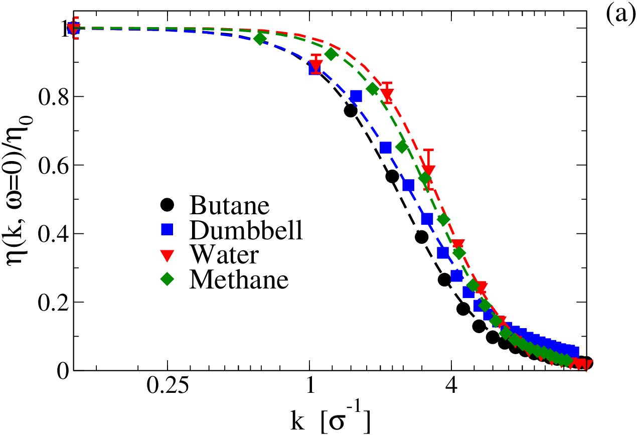

One immediately notices that for the wave vector dependent viscosity approaches the zero wave vector limit. This is in good agreement with the Bocquet-Charlaix criterion, Eq. (24). Interestingly, this is independent of the specific fluid studied here and the local constitutive relations can be applied on length scales down to approximately 2-2.5 nm.
Is this a general result that applies to all fluidic systems? The answer is no! In Fig. 4 (b) the zero-frequency viscosity kernel is plotted for the asymmetric dumbbell model for different temperatures. The asymmetry arises due to the mass and Lennard-Jones parameter differences between the two constituent atoms. The asymmetric dumbbell model allows one to probe the dynamics in the highly viscous regime without crystallization occurring [52]. The result shows that for relatively high temperatures the kernel has the same wave vector dependency, but approaching the viscous regime (lower temperature) the kernel only reaches the Newtonian viscosity at longer length scales. This indicates that the dynamical processes behind the viscous response take place on longer length scales in accordance with the cooperative motion in super-cooled liquids [53]. The non-local viscous response has also been studied for highly viscous two component Lennard-Jones system and polymer melts, see Refs. 31, 32.
The failure of the local constitutive relation, that is, of Newton’s law of viscosity, is very clearly illustrated by Todd et al. [54] for a point-mass Weeks-Chandler-Andersen (WCA) system [55]. In real space the non-local description amounts to a convolution of the viscosity kernel and the strain rate distribution, Eq. (26). In the homogeneous situation where the fluid undergoes a steady shear in the -direction with varying amplitude in the -direction we have one non-zero shear component in the pressure tensor, namely, the component. In this steady situation Eq. (26) reduces to
| (30) |
where . If the shear is induced by an external force field , the fluid flow is , where is the excited Fourier mode of the velocity field. We assume that this is the only mode excited, i.e., the force amplitude must be sufficiently low [56]. Also, this ensures a linear response as well as constant temperature and density. The strain rate is then
| (31) |
For simplicity we shall assume that the kernel is given by a Gaussian function
| (32) |
such that gives a characteristic decay length. The kernel must fulfill [54] (i) , and (ii) is an even function. Substituting Eqs. (31) and (32) into Eq. (30) we have upon integration
| (33) |
If the model is local, corresponding to Newton’s law of viscosity, that is, for the local model
| (34) |
The system can be simulated using the Sinusoidal Transverse Force (STF) method [57], and it is possible to evaluate for different external force fields and wave vectors. The two different predictions can be compared to the actual shear pressure , which is found directly from the momentum balance equation that for the steady flow reads
| (35) |
Integrating we obtain
| (36) |
The comparison is made in Fig. 5. Clearly, the local prediction fails for the larger wave vector, Fig. 5 (b), whereas the non-local prediction agrees with the actual shear pressure. From the non-local model we conclude that spatial correlations result in a reduced shear pressure.


From Eqs. (33) and (34) we can quantitatively evaluate the effect of spatial correlations on the stress. Specifically, we have the relative difference given by
| (37) |
For the WCA system studied here and the Bocquet-Chairlaix criterion gives , this corresponds to an error in the stress below 32 % according to Eq. (37).
The Gaussian function does not perfectly fit to the kernel data. Nevertheless, this simple functional form captures the non-local response well, due to the smoothing of the convolution. Other more complicated forms have been suggested, see Refs. 51, 31, 58.
Todd and Hansen [59] showed that the non-local response is only relevant for flows where the strain-rate is non-linear with respect to position. Couette and Poiseuille flows are then not affected by non-locality. To illustrate this consider any functional form for the kernel which fulfills the criteria given above: its integral gives the zero wave vector viscosity and it is an even function with respect to . First, making the change of variables Eq. (30) reads
| (38) |
Assuming a strain rate on the form , we have
| (39) |
as the integrand in the second integral is an odd function. This result is the same as the local prediction. In general, if a Taylor expansion of the strain rate exists, using the properties of odd and even functions one can verify that the non-zero non-local effects of the strain rate can be determined by the even moments of the kernel [59]
| (40) |
In the case of Couette and Poiseuille flows the Taylor expansion terminates at zero’th and first order, respectively, and there are no non-local effects.
The spin and rotational viscosity kernels can be found by simply rearranging Eq. (19c) giving the generalized susceptibility
| (41) |
Our group recently [42, 43] conjectured that the rotational viscosity governs the fast wave vector independent relaxation processes as indicated in Figs. 2 (a) and 3 (a). This transport coefficient is therefore only frequency dependent. We then have
| (42) |
and therefore
| (43) |
We called this the generalized extended Navier-Stokes (GENS) theory. From MD simulations one can calculate the LAVACF (as shown above) and from there find the kernels. For dense fluids is characterized by a sharp peak around zero wave vector [42] since the diffusive contribution to the relaxation of the LAVACF is very small for , see Figs. 2 (a) and 3 (a). The spin viscosity kernel has the same properties as the shear viscosity kernel and for this reason we do not expect any non-local effects for flows where the gradient of the angular velocity is constant or linear.
IV Nanoflows
IV.1 The Poiseuille flow
We first study a Poiseuille flow, the geometry is shown in Fig. 1. In experiments this flow can be achieved by application of a constant pressure gradient. Generating a pressure difference in simulations with, for example, a piston and using molecular reservoirs can cause density variations in the direction of the flow and other inlet/outlet effects. We therefore use a constant force field acting on each point mass in the fluid to drive the flow. The wall particles are arranged on a simple cubic lattice and are allowed to vibrate around their initial lattice site using a simple restoring spring force. The viscous heating generated in the fluid is removed by thermostating the wall particles. This method resembles the real physical experiment and is therefore often referred to as direct non-equilibrium molecular dynamics. The interested reader is referred to Ref. [11] for further details. To get a satisfactory signal-to-noise ratio in the MD simulations unrealistically large external forces are typically applied to drive the system, and the resulting flow rates are very large, typically, in the order of 10-100 m s-1. Despite these large flow rates the Reynolds number is usually less than unity due to the extremely small characteristic length scales involved. Finally, it is very important to ensure that the simulations are carried out in the linear regime which is discussed below.
IV.1.1 Continuum predictions
In the linear regime of low Reynolds number and for the geometry shown in Fig. 1 the ENS equations form a two-point boundary value problem in the steady state
| (44a) | ||||
| (44b) | ||||
where . Recall that and . Introducing and applying no-slip boundary conditions, and , Eringen [23] solved this yielding
| (45a) | ||||
| (45b) | ||||
with the following definitions of and
| (46) |
The application of the no-slip boundary condition is not justified. A correct treatment applies the Neumann boundary condition for both the velocity and angular velocity fields, however, this is not straightforward in that the two are likely coupled and therefore dependent on each other. While the boundary condition for the velocity field has been studied in great detail, see e.g. Refs. [60, 61, 62], very little is known about the spin boundary condition. Just recently De Luca et al. [63] showed that the spin field does possess slippage and Badur et al. [64] used spin slip to account for flow enhancement. As mentioned in the introduction, we will treat the problem in an ad hoc fashion and simply set the angular velocity slip in accordance with the MD data.
If one ignores the coupling, , the solution for the streaming velocity, Eq. (45a), reduces to the classical Poiseuille flow solution
| (47) |
In this classical situation the angular velocity is found from the vorticity, , that is,
| (48) |
in agreement with Eq. (45b) for . As the classical treatment does not allow for specification of spin boundary condition, Eqs. (45b) and (48) differ by a magnitude of at the walls.
From Eq. (45a) one can see that the maximum velocity, located at , is lowered as a result of the coupling since from the last term we have and thus . Another way to quantify this effect is to evaluate the volumetric flow rate [3]
| (49) |
where is the characteristic half length in the -direction. This gives the relative volumetric flow rate reduction
| (50) |
Equation (50) is plotted in Fig. 6 for the dumbbell fluid, liquid butane, and water. The relevant coefficients can be found in SI Table I. It can be seen that for water flowing in a channel with a width of 9 nm the flow rate is reduced by about 10 % due to the coupling. As the channel width increases the flow rate approaches that of the classical predictions and the effect of the coupling can be ignored.

From Eq. (50) the relative flow rate reduction increases as the product decreases. From this observation, one can define a characteristic fluid length scale [65] below which the effect of the coupling becomes significant. To this end we write the parameter as
| (51) |
From SI Table I it is seen that and . Thus a significant flow-rate reduction occurs for fluids with large critical length scale . For water nm and for butane nm in agreement with the relative large flow rate reduction observed for water.
IV.1.2 Comparison with molecular dynamics simulations
First we compare MD data with continuum predictions for the dumbbell system. Before the comparison, however, the linear Newtonian response regime should be identified, at least, for the bulk fluid region. To this end one can apply the synthetic SLLOD algorithm developed by Evans and Morris [66]. Basically the method imposes a constant strain rate (linear velocity profile) on the system while ensuring a homogeneous density and iso-kinetic temperature. To achieve this the equations of motion are reformulated according to the Gaussian principle of least constraint, see also Refs. 3, 4. Performing a series of SLLOD simulations it is found that the Newtonian regime occurs in the range for the dumbbell fluid . The upper limit for the external force field can then be approximated by rewriting Eq. (48) to giving , with . Note, in the wall-fluid region the velocity may feature rapid changes and here the linearity is not guaranteed.
Based on the SLLOD approach Delhommelle [67] developed a synthetic method to calculate the rotational viscosity as a function of spin angular velocity. See also Edberg et al. [68]. To our knowledge no synthetic or controlled method exists to study the spin viscosity dependency of the gradient of the spin, or the rotational viscosity dependency on strain rate. We will therefore here assume that the linear regime is identical to the Newtonian regime, i.e., in the regime where the viscosity is independent of the strain rate.
The classical description predicts that the Poiseuille flow is local flow according to Sec. III. Also, from Fig. 6 we expect the flow-rate reduction due to the coupling to be very low for the dumbbell model. Thus, based on the theory we can expect the classical description to be a good approximation for this system. The time-averaged velocity and spin angular velocity profiles are shown in Fig. 7 (a) for the dumbbell model where the pore width is approximately 14.8 atomic diameters. The profiles are sampled after the system has reached the steady state. The temperature profile (not shown) is constant and the temperature is throughout the channel.


The predictions from the classical Navier-Stokes theory, Eqs. (47) and (48), are also plotted using the shear viscosity from SI Table I. Velocity slippage at the wall-fluid interface is allowed, ; is then the only fitting parameter in the comparison. The agreement between MD data and classical continuum predictions is excellent, except at the wall-fluid interface. This is highlighted by the shear pressures plotted in Fig. 7 (b). According to the classical theory the shear pressure is linear, however, at the wall-fluid interface this is not the case. Also, the classical theory assumes a zero anti-symmetric part of the shear stress . This is clearly not fulfilled near the wall.
To understand the disagreement at the boundary, we analyze the fluid ordering. It is well known that the wall induces a density variation in the fluid [69]. The density profile is shown in Fig. 7 (c) (black dots). It is seen that the density varies in a region approximately one atomic diameter away from the wall. The transport properties are functions of density, and one should expect a variation in the viscosities here. Furthermore, one can evaluate the molecular alignment ordering through the parameter [70]
| (52) |
where is the angle between the molecular bond and -plane. For perfect parallel alignment , that is, the molecules closest to the wall are, on average, aligned with the wall. For distances around one atomic diameter the molecules are slightly normal to the wall as . The extremes are illustrated with the two molecules in the lower left corner in Fig. 7(c). For zero order parameter, the molecules have random orientations which is the case in the interior of the channel. This means that the system possesses a degree of anisotropy in the wall-fluid region. To fully account for the density variation and ordering one should therefore describe the transport properties through a position-dependent tensorial shear viscosity.
Figure 8 (a) shows the velocity and density profiles for a butane flow where the pore width is just 6 nm. For such extreme confinements the fluid layering stretches over the entire pore. The order parameter profile, Fig. 8 (b), shows that the molecular orientation is strongly anisotropic. Finally, the mean square molecular end-to-end distance also varies, showing that the butane molecule on average is elongated at the fluid-region by around 2 per cent. Such a complex system is not modeled appropriately by the classical or extended theories presented here. This is not an indication of a breakdown of the continuum picture, but an incomplete modeling. Worth noting is that the fluid ordering and layering is constant over a large range of external forces including zero force, see Fig. 8, and is thus not flow induced.


As pointed out by Bitsanis et al. [71] the velocity profile features surprisingly small modulations considering the density profile: one should expect the transport properties to vary significantly across the channel having large effects on the flow profile. The authors suggested the local average density model (LADM) wherein the transport properties at a point is a function of the average density around that point. In the current geometry, where the density is constant in the plane parallel to the wall, the local average is
| (53) |
where defines the region of averaging. The agreement between the LADM and simulation data can be very good, especially if one introduces a non-uniform weighting function [72]. However, the LADM cannot predict the shear pressure response in Fig. 5 as the density is constant. Also, the LADM model is not capable of predicting the strain rate reversal observed by Travis et al. [11, 73]
To account for the observed velocity profile one can write the position-dependent (in-homogeneous) non-local constitutive model as
| (54) |
The position dependency likely comes from the varying density at the wall-fluid region. The application of this relation is not straightforward [74, 75] as it is unclear how the convolution should be performed at the wall where the support of the kernel goes beyond the boundary and is unknown [74, 75]. Recently, Dalton et al.[76] used a sinusoidal longitudinal force (SLF), also introduced by Hoang and Galliero [72], to control the density variation in a periodic system. Due to the periodicity, the boundary problem can be eliminated. The density profile can be controlled to such an extent that it resembles that seen in confined systems. The fluid can then be driven by an STF. The authors showed that the non-local response is capable of predicting the strain rate reversal observed by Travis et al. [11, 73], as well as the relative small modulation on the velocity profile. A rigorous and general implementation of Eq. (54) into the balance equations for confined systems is still lacking.
For the dumbbell and butane models the coupling between the linear and spin angular velocities has little effect on the flow. From Fig. 6, however, the effect is significant for water flow in channel with widths below 5 nm. In Fig. 9 (a) MD data for the velocity profile for water is plotted where the channel width is approximately 10 water diameters.


Also, shown are the predictions from the classical NS and ENS theories. Density and order parameter profiles (not plotted here) show little density variation and molecular alignment, except within 3-4 Å of the wall. The slip velocities are estimated by fitting a second-order polynomial (dashed lines) to the velocity profile, excluding the wall-fluid region where the fluid is slightly anisotropic and inhomogeneous; this then amounts to the apparent slip length [77] and is the only fitting parameter used in the comparison. It is seen that the classical prediction fails, while the ENS theory captures the flow profile Note, fit of the profile data to the classical description will result in a wrong viscosity no matter how many data points in the wall-fluid region are included. Any shift of the profile will not change this either. An extra source of dissipation must be present. Furthermore, note that a complete description involves a position dependent non-local anisotropic modelling of the wall-fluid region.
To remove any effect in the boundary region one can evaluate the curvature in the channel midpoint, . The predictions are simply found from the second-order derivative of Eqs. (45a) and (47). The relative difference is
| (55) |
is plotted in Fig. 9 (b) together with the results from the MD simulations. Within statistical uncertainty the ENS theory and MD simulation results agree. As the channel width increases the relative curvature difference vanishes and the classical description is re-captured.
The particular model applied is parameterized with respect to the liquid state and the wall is a Lennard-Jones cubic lattice, see Ref. 9. The fluid structure near the wall and its effect on the dynamics will be affected by the different models, choice of model parameters, and wall details. However, it is not the aim here to critically review the fluid structure at near the wall, but to see the effect of the coupling.
IV.2 Inserting torque
Perhaps the most clear illustration of the translational-rotational coupling is seen by introducing an external torque into the system while having a zero production term for the linear momentum. In general, if the resulting torque density is sufficiently small then for the geometry in Fig. 1 we have
| (56a) | ||||
| (56b) | ||||
Integrating Eq. (56a) we get in terms of which is substituted into Eq. (56b) resulting in a second order inhomogeneous differential equation for . From this and Eq. (56a) and by application of Dirichlet no-slip boundary conditions one has
| (57a) | ||||
| (57b) | ||||
where and are integration constants. One can show that goes rapidly to zero as increases. In this limit the spin angular velocity is
| (58) |
and velocity profile is linear with a slope given by the last term in Eq. (57a). Figure 10 depicts the two profiles for the butane liquid using m2s-2.

From this one sees that the external torque produces a significant local flow; the average flow is zero due to the system symmetry.
In 2009 Bonthuis et al. [78] showed that the coupling between the linear momentum and spin could be exploited in order to pump water through carbon nanotubes by application of a rotating field. The was theory based on the ENS equations at it was noted that in order to obtain a non-zero mean flow asymmetric boundary conditions must be employed which can be achieved by confining the fluid between two walls with different hydrophobicity in the case of water pumping. Recently De Luca et al. [63] performed extensive MD simulations of the mechanism under experimentally feasible conditions, indicating that the mechanism is functional. This could prove to be a way to overcome the large hydraulic resistance characterizing nanofluidic flows. Felderhof showed in 2011 that the coupling can also be utilized to perform plane-wave pumping [79] and even propel microrobots [80].
V Summary
We have derived the relevant dynamical equations for isotropic nanofluidic flows. The formulation is based on the basic definition of a macroscopic field variable from the corresponding microscopic or molecular variable, and it includes the underlying molecular structure. Two intrinsic nanofluidic phenomena were discussed, namely, (i) the coupling between the spin angular momentum and (ii) the linear momentum and the non-local fluid response. The important points are the following.
(1) The effect of the coupling between the linear and spin angular velocities can be estimated through the characteristic length scale , Eq. (51). For large significant flow rate reduction is observed, partly explaining the “increased” or “effective” viscosity reported in the literature. Other effects, like anisotropy, will also play a role in the change in effective transport properties. For polar molecular systems like water nm, and the coupling must be considered on these length scales. For the non-polar fluids studied here is below 1 nm and the coupling effect is very small in most situations.
(ii) In general any fluid response can be described phenomenologically through a transport kernel that incorporates the spatial and temporal correlation effects. A method for calculating the shear viscosity kernel was presented. This showed that for non-highly viscous fluids the Newtonian limit is reached on length scales of a few nanometers. This is in agreement with the Bocquet-Charlaix criterion if the decay time for the stress autocorrelation function is applied as the relaxation parameter. Importantly, non-local effects are not present in simple flows where the strain-rate is linear with respect to spatial coordinate, which is the case for Couette and Poiseuille flows. For non-linear flows the non-local response significantly affects the fluid stress for strain-rate variations on the atomic length scale.
(iii) For highly confined fluids molecular alignment phenomena and molecular deformation can occur along with the fluid layering, see Fig. 8. Simple classical continuum theory does not include or account for such complex fluid structure. It would be interesting to investigate this is more detail, for example, using the theory for liquid crystals [70, 81].
In conclusion, continuum theory is applicable even on the nanoscale if the relevant physical processes are modelled appropriately.
Acknowledgement
The authors wish to acknowledge Lundbeckfonden for supporting this work as part grant no. R49-A5634. The centre for viscous liquid dynamics “Glass and Time” is sponsored by the Danish National Research Foundation (DNRF).
References
- [1] J.C.T. Eijkel and A. van den Berg. Nanofluidics: what is it and what can we expect from it? Microfluidics Nanofluidics, 1:249–267, 2005.
- [2] L. Bocquet and E. Charlaix. Nanofluidics, from bulk to interface. Chem. Soc. Rev., 39:1073, 2010.
- [3] H. Bruus. Theoretical Microfluidics. Oxford University Press, 2008.
- [4] F. Persson, L. H. Thamdrup, M. B. L. Mikkelsen, P. Skafte-Pedersen S. E. Jaarlgard, H. Bruus, and A. Kristensen. Double thermal oxidation scheme for the fabrication of SiO2 nanochannels. Nanotechnology, 18:245301, 2007.
- [5] L.D. Landau and E.M. Lifshitz. Fluid Mechanics, 2nd edition. Elsevier, Amsterdam, 1987.
- [6] D.J. Tritton. Physical Fluid Dynamics. Oxford Science Publications, 1988.
- [7] B. Lautrup. Physics of Continuous Matter. Institute of Physics Publishing, Bristol, 2005.
- [8] R. L. Rowley and M. M. Painter. Diffusion and viscosity equation of state for a Lennard-Jones fluid obtained from molecular dynamics simulations. Int. J. Therm. Phys., 18:1109, 1997.
- [9] J.S. Hansen, J.C. Dyre, P.J. Daivis, B.D. Todd, and H. Bruus. Nanoflow hydrodynamics. Phys. Rev. E, 84:036311, 2011.
- [10] L. H. Thamdrup, F. Persson, H. Bruus, H. K. Flyvbjerg, and A. Kristensen. Experimental investigation of bubble formation during capillary filling of SiO2 nanoslits. Appl. Phys. Lett., 91:163505, 2007.
- [11] K. P. Travis, B. D. Todd, and D. J. Evans. Depature from Navier-Stokes hydrodynamics in confined liquids. Phys. Rev. E, 55:4288–4295, 1997.
- [12] F. Detcheverry and L. Bocquet. Thermal fluctuations in nanofluidic transport. Phys.Rev.Lett, 109:024501, 2012.
- [13] S.A. Gupta, H.D. Cochran, and P.T. Cummings. Nanorheology of liquid alkanes. Fluid Phase Eq., 150-151:125, 1998.
- [14] G. Karniadakis, A. Beskok, and N. Aluru. Microflows and Nanoflows: Fundamentals and Simulation. Springer, New York, 2005.
- [15] G. Lukaszewics. Micropolar Fluids: Theory and Applications. Birkhauser, Boston, 1999.
- [16] V.A. Eremeyev, L.P. Lebedev, and H. Altenbach. Foundation of Micropolar Mechanics. Springer, 2013.
- [17] E. Cosserat and F. Cosserat. Sur la théorie de l’esticité. Ann. Toulouse, 10:1, 1896.
- [18] E. Cosserat and F. Cosserat. Théorie des corps d’eformables. Hermann, 1909.
- [19] A.M. Sonnet, P.L. Maffettone, and E.G. Virga. Continuum theory for nematic liquid crystals with tensorial order. J. Non-Newtonian Fluid Mech., 119:51, 2004.
- [20] P. Muthu, B.V. Rathish Kumar, and P. Chandra. A study of micropolar fluid in an annular tube with application to blood flow. J. Mech. Med. Biol., 8:561, 2008.
- [21] H. Grad. Statistical mechanics, thermodynamics and fluid dynamics of systems with an arbitrary number of integrals. Comm. Pure. Appl. Math., 5:455, 1952.
- [22] J.S. Dahler and L.E. Scriven. Theory of structured continua i. general considarations of angular momentum and polarization. Proc. R. Soc. Lond. A, 27:504, 1963.
- [23] A. C. Eringen. Contribution to mechanics. Oxford, 1969. Pergamon, editor D. Abir.
- [24] S. R. de Groot and P. Mazur. Non-equilibrium Thermodynamics. Dover Publications, 1984.
- [25] R. F. Snider and K. S. Lewchuk. Irreversible thermodynamics of a fluid system with spin. J. Chem. Phys., 46:3163, 1967.
- [26] N. K. Ailawadi, B. J. Berne, and D. Forster. Hydrodynamics and Collective Angular-momentum Fluctuations in molecular Fluids. Phys. Rev. A, 3:1462–1472, 1971.
- [27] D. J. Evans and W. B. Streett. Transport properties of homonuclear diatomics II. Dense fluids. Mol. Phys., 36:161–176, 1978.
- [28] W. E. Alley and B. J. Alder. Generalized transport coefficients for hard spheres. Phys. Rev. A, 27:3158, 1983.
- [29] J.P. Boon and S. Yip. Molecular Hydrodynamics. Dover Publication, New York, 1991.
- [30] D. J. Evans and G. P. Morriss. Statistical Mechanics of Nonequilibrium Liquids. Academic Press, 1990.
- [31] A. Furukawa and H. Tanaka. Nonlocal nature of the viscous transport in supercooled liquids: Complex fluid approach to supercooled liquids. Phys. Rev. Lett., 103:135703, 2009.
- [32] R.M. Puscasu, B.D. Todd, Peter J. Daivis, and J.S Hansen. Nonlocal viscosity of polymer melts approaching their glassy state. J. Chem. Phys., 133:144907, 2010.
- [33] M. P. Allen and D. J. Tildesley. Computer Simulation of Liquids. Clarendon Press, New York, 1989.
- [34] Y. Wu, H. L. Tepper, and G. A. Voth. Flexible simple point-charge water model with improved liquid-state properties. J. Chem. Phys., 124:024503, 2006.
- [35] J.-P. Ryckaert and A. Bellemans. Molecular Dynamics of Liquid Alkanes. Faraday Discuss. Chem. Soc., page 95, 1978.
- [36] J.Wang, R.M. Wolf, J.W. Caldwell, P.A.Kollman, and D.A. Case. Development and Testing of a General Amber Force Field. J. Comp. Chem., 25:1157, 2004.
- [37] J.S. Hansen. https://code.google.com/p/seplib/.
- [38] J. A. Thomas and J. H. McGaughey. Reassessing Fast Water Transport Through Carbon Nanotubes. Nano Lett., 8:2788–2793, 2008.
- [39] M. Whitby, L. Cagnon, M. Thanou, and N. Quirke. Enhanced fluid flow through nanoscale carbon pipes. Nan. Lett., 8:2632, 2008.
- [40] J.H. Irving and J.G. Kirkwood. The statistical mechanical theory of transport processes. iv. the equations of hydrodynamics. J. Chem. Phys., 18:817–829, 1950.
- [41] B. D. Todd and P. J. Daivis. Homogeneous non-equilibrium molecular dynamics simulations of viscous flow: techniques and applications. Mol. Sim., 33:189, 2007.
- [42] J.S Hansen, P.J. Daivis, J.C. Dyre, B.D. Todd, and H. Bruus. Generalized extended Navier-Stokes theory: Correlations in molecular fluids with intrinsic angular momentum. J. Chem. Phys., 138:034503, 2013.
- [43] J.S Hansen. Generalized extended navier-stokes theory: Multiscale spin relaxation in molecular fluids. Phys. Rev. E, 88:032101, 2013.
- [44] L.P. Kadanoff and P.C. Martin. Hydrodynamic Equations and Correlation Functions. Ann. Phys., 281:800, 2000.
- [45] L. Onsager. Reciprocal relations in irreversible processes. I. Phys. Rev., 37:405, 1931.
- [46] J.M.O. de Zárate and J.V. Sengers. Hydrodynamic Fluctuations. Elsevier, Amsterdam, 2006.
- [47] S. Sarman. Flow properties of liquid crystal phases of the gay-berne fluid. J. Chem. Phys., 108:7909, 1998.
- [48] R. J. D. Moore, J. S. Hansen, and B. D. Todd. Rotational viscosity of linear molecules: an equilibrium molecular dynamics study. J. Phys. Chem., 128:224507, 2008.
- [49] R. Hartkamp, P.J. Daivis, and B.D. Todd. Density dependence of the stress relaxation function of a simple liquid. Phys. Rev. E, 87:0321551, 2013.
- [50] R.M. Puscasu, B.D. Todd, Peter J. Daivis, and J.S Hansen. An extended analysis of the viscosity kernel for monatomic and diatomic fluids. J. Phys.: Condens. Matter, 22:195105, 2010.
- [51] J. S. Hansen, P. J. Daivis, K. P. Travis, and B. D. Todd. Parameterization of the nonlocal viscosity kernel for an atomic fluid. Phys. Rev. E, 76:041121, 2007.
- [52] T.B. Schrøder, U.R. Pedersen, N.P. Bailey, S. Toxvaerd, and J.C. Dyre. Hidden scale invariance in molecular van der waals liquids: A simulation study. Phys. Rev. E, 80:041502, 2009.
- [53] A. Cavagna. Supercooled liquids for pedestrians. Phys, Rep., 476:51, 2009.
- [54] B. D. Todd, J. S. Hansen, and P.J. Daivis. Nonlocal shear stress for homogeneous fluids. Phys. Rev. Lett., 100:195901–195904, 2008.
- [55] J. D. Weeks, D. Chandler, and H. C. Andersen. Role of repulsive forces in determining the equilibrium structure of simple liquids. J. Chem. Phys., 54:5237–5247, 1971.
- [56] J. S. Hansen, P. J. Daivis, and B. D. Todd. Local linear viscoelasticity of confined fluids. J. Chem. Phys., 126:144706, 2007.
- [57] E. M. Gosling, I. R. McDonald, and K. Singer. On the calculation by molecular dynamics of the shear viscosity of a simple fluid. Mol. Phys., 26:1475, 1973.
- [58] K.P. Travis, D.B. Searles, and D. Evans. On the wavevector dependent shear viscosity of a simple fluid. Mol. Phys., 97:415, 1999.
- [59] B. D. Todd and J. S. Hansen. Nonlocal viscous transport and the effect on fluid stress. Phys.Rev.E, 78:051702, 2008.
- [60] C. L. M. H. Navier. Memoire sur les lois du mouvement des fluids. Memoires de l’Academic Royale des Sciences de l’Institut de France, 6:389–440, 1823.
- [61] L. Bocquet and J.-L. Barrat. Hydrodynamic boundary conditions, correlations functions, and Kubo relations for confined fluids. Phys. Rev. E, 49:3079–3092, 1994.
- [62] J.S. Hansen, B.D. Todd, and P.J. Daivis. Prediction of fluid velocity slip at solid surfaces. Phys. Rev. E, 84:016313, 2011.
- [63] S. De Luca, B.D. Todd, J.S. Hansen, and P.J. Daivis. Molecular dynamics study of nanoconfined water flow driven by rotating electric fields under realistic experimental conditions. Langmuir, 30:3095, 2012.
- [64] J. Badur, P. Ziolkowski, and P. Ziolkowski. On the angular velocity slip in nano-flows. Microfluid Nanofluid, 2015.
- [65] J.S. Hansen, P. J. Daivis, and B. D. Todd. Viscous properties of isotropic fluids composed of linear molecules: Departure from the classical Navier-Stokes theory in nano confined geometries. Phys. Rev. E, 80:046322, 2009.
- [66] D. J. Evans and G. P. Morris. Nonlinear-response theory for steady planar couette flow. Phys. Rev. A., 30:1528, 1984.
- [67] J. Delhommelle. Rotational viscosity of uniaxial molecules. Mol. Phys., 100:3479–3482, 2002.
- [68] R. Edberg, G. P. Morriss, and D. J. Evans. Rheology of -alkanes by nonequilibrium molecular dynamics. J.Chem.Phys, 86:4555, 1987.
- [69] S. Toxvaerd. The structure and thermodynamics of a solid-fluid interface. J. Chem. Phys., 74:1998–2005, 1981.
- [70] P.G.D. Gennes and J. Prost. The Physics of Liquid Crystals. Claredon Press, 1993.
- [71] I. Bitsanis, T.K. Vanderlick, M. Tirrell, and H.T. Davis. Tractable molecular theory of flow in strongly inhomogeneous fluids. J. Chem. Phys., 89:3152, 1988.
- [72] H. Hoang and G. Galliero. Shear viscosity of inhomogeneous fluids. J. Chem. Phys., 136:124902, 2013.
- [73] K. P. Travis and K. E. Gubbins. Poiseuille flow of lennard-jones fluids in narrow slit pores. J. Chem. Phys., 112:1984, 2000.
- [74] J. Zhang, B.D. Todd, and K.P. Travis. Viscosity of confined inhomogeneous nonequilibrium fluids. J. Chem. Phys., 121:10778–10786, 2004.
- [75] P. J. Cadusch, B. D. Todd, J. Zhang, and P. J. Daivis. A non-local hydrodynamic model for the shear viscosity of confined fluids: analysis of homogeneous kernel. J.Phys. A, 41:035501, 2008.
- [76] B.A. Dalton, P.J. Daivis†, J.S. Hansen, and B.D. Todd. Effects of nanoscale density inhomogeneities on shearing fluids. Phys. Rev. E, 88:052143, 2013.
- [77] E. Lauga M. Brenner and H. Stone. Microfluidics: The no-slip boundary condition. In C. Tropea, A.L. Yarin, and J.F. Foss, editors, Springer Handbook of Experimental Fluid Mechanics. Springer, 2007.
- [78] J. D. Bonthuis, D. Horinek, L. Bocquet, and R. R. Netz. Electrohydraulic power conversion in planar nanochannels. Phys. Rev. Lett., 103:144503, 2009.
- [79] B. U. Felderhof. Efficiency of magnetic plane wave pumping of a ferrofluid through a planar duct. Phys. Fluids, 23:092003, 2011.
- [80] B. U. Felderhof. Self-propulsion of a planar electric or magnetic microbot immersed in a polar viscous fluid. Phys. Rev. E, 83:056315, 2011.
- [81] S. Sarman and D.J. Evans. Statistical mechanics of viscous flow in nematic fluids. J. Chem. Phys., 99:9021–9036, 1993.
Supporting Information
Balance equations and the Extended Navier-Stokes equation
A macroscopic field variable is be given by the corresponding microscopic quantity associated with molecule through [1]
| (59) |
where is the Dirac delta function and is the molecular center-of-mass position. In our treatment can be a scalar quantity (e.g. the mass density) or a vector quantity (e.g. the momentum density). In Fourier space we have for
| (60) |
From now on we do not write the time and position dependencies of the free variables (right hand side of the equations) explicitly unless it provides important information. The rate of change in Fourier space is given by
| (61a) | ||||
| (61b) | ||||
where is the center-of-mass velocity. The following identity has been applied, where is a scalar or a vector
| (62) |
In the situation where is a vector the product is the dyadic between two vectors, and , and the resultant is the second rank tensor with components , . The dyadic is not commutative, i.e., , unless is symmetric. The dyadic is also called the outer product and sometimes written as . If and are parallel the dyadic is symmetric. To first order in wave vector Eq. (61b) becomes
| (63) |
The particle velocity can be decomposed into a thermal (or ”peculiar”) term and advective term by
| (64) |
is the mass averaged fluid velocity in a region around . This region is equivalent to the fluid particle volume encountered in the traditional continuum description [2] as was briefly discussed in the introduction. We assume that the thermal and advective velocities are uncorrelated and the thermal motion is, by definition, conserved with , where is the mass. From this Eq. (63) becomes
| (65) |
where is a linear operator given by
| (66) |
is henceforth refered to as the “microscopic hydrodynamic operator” (MH-operator) since it describes the microscopic interpretation of the fluid’s dynamics in the hydrodynamic regime of small wave vectors. The first term describes the rate of change of the microscopic quantity in question, the second and third terms are then the thermal and advective contributions to the dynamics, respectively. We proceed and apply Eqs. (65) and (66) to express the balance equations of mass, linear momentum and angular momentum.
V.1 Mass balance
The mass density field is defined directly from Eq. (59) as [3]
| (67) |
The MH-operator acting on gives
| (68a) | ||||
| (68b) | ||||
since the mass of each particle is constant and . The dynamics in Fourier space is thus simply
| (69) |
Relating to the general balance equation, Eq.(1) in the manuscript, in the case of zero production term, one has , and no surface forces
| (70) |
In Fourier space this yields
| (71) |
using that , which follows from partial integration of Eq.(60). In the limit of small wave vector we thus identify Eq. (69) as the microscopic interpretation of the continuous mass balance equation.
V.2 Linear momentum
In general, there is no microscopic definition of the streaming velocity in the form of Eq. (59) [3]. Rather, the linear fluid motion is given through the momentum density . Note, Hansen and McDonald [1] define a current from the microscopic velocities and Eq. (59), which is then the correct mass weighted averaged streaming velocity for single species fluids. If is the linear momentum of particle we have
| (72) |
Applying the MH-operator we have
| (73a) | ||||
| (73b) | ||||
as it can be shown [4] that the cross terms since the thermal and advective velocities are uncorrelated.
is the total force acting on molecule . This force is decomposed into the force on due to interactions with all other molecules denoted henceforth by and external forces , i.e., . The first term on the right hand side of Eq. (73b) is
| (74) |
using Newton’s third law and the identity Eq. (62). Substituting this into Eq. (73b) and rearranging one arrives at
| (75) |
where
| (76) |
We recognize Eq. (75) as the balance equation for linear momentum in Fourier space. Importantly, the last term on the right hand side gives one possible microscopic interpretation of the pressure tensor in the zero wave vector limit [4]. Let be the system volume. Then according to Eq. (1) in the manuscript and (75) we have for the zero wave vector pressure tensor
This is the Irving-Kirkwood interpretation [5] and will be discussed in the following.
The configurational part of the pressure tensor is the term and can be written in a different form assuming pairwise additive interactions only. Using Newton’s third law once again, , where is the force on due to interactions with , we get
| (77) |
where . The Irving-Kirkwood pressure tensor then reads
| (78) |
At this point we emphasize the difference between the atomic and molecular formalisms. If particles and represent point-masses (including atoms in the molecules), rather than structured molecules, the vectors and are parallel, the dyadic is symmetric. This implies that the pressure tensor is symmetric. In the case of structured molecules, however, the force on molecule due to is given by
| (79) |
where indices and represent atom in molecule and atom in molecule , see Fig. 11. The force needs not be parallel to the vector connecting the molecules’ center-of-masses and the configurational part of the pressure tensor is not generally symmetric.

There is no ambiguity between the two formalisms. They are trivially equivalent for point-mass particles, and for structured molecules one can be expressed in terms of the other and the mass dispersion tensor [6, 4]. The two formalisms provide different information and we use the molecular one here. We use the term ’atom’ loosely: it represents a point-mass spherical particle, and can be a single atom or a united group of atoms like the methyl group.
In the molecular formalism the pressure tensor decomposes into a sum of the symmetric and anti-symmetric parts such that with
| (80) |
Following Evans and Morriss [3] we here use the stack notation to indicate the symmetric and anti-symmetric parts. The symmetric part can be further decomposed into a sum of the equilibrium pressure , the viscous pressure , and the trace-less symmetric tensor [3]
| (81) |
where is the second rank identity tensor and . The anti-symmetric part of the pressure tensor has zero diagonal components and three independent off-diagonal components. It is therefore often written as a (pseudo) vector dual of the tensor. Here the subscripts indicate the tensor components. From the definition of , Eq. (80), one has for
| (82) | |||||
Here and are the unit vectors along the -, - and -axes, respectively. From Eq. (82) it is clear that the anti-symmetric pressure is associated with the torque on about and gives rise to a change of orbital angular momentum, i.e., that of the center-of-mass motion of the molecules. Importantly, when the pressure tensor has a non-zero anti-symmetric part, the orbital angular momentum is a non-conserved quantity [7]; we address this in the following. Conservation of orbital angular momentum is sometimes used as an argument for a symmetric pressure, see for example Aris [8], but note that later Aris also allows for the possibility of asymmetry. Finally, notice that the kinetic part of the pressure tensor is a symmetric dyadic and does not enter the anti-symmetric part.
V.3 Orbital and spin angular momenta
Consider now the case when no external forces are present. Following the approach for the linear momentum we write the orbital angular momentum density as
| (83) |
where is the orbital angular momentum per unit mass, and is the orbital angular momentum of molecule . Note, the angular momentum is defined with respect to some specific choice of coordinate system. The MH-operator acting on gives
| (84a) | ||||
| (84b) | ||||
where is the torque on molecule and is the sum of torques
| (85) |
The torque does not sum to zero as the orbital angular momentum is a non-conserved quantity [7]. Rather it is the total angular momentum, i.e., the sum of orbital and spin (or intrinsic) angular momenta, which is conserved. For point-masses spin angular momentum is not present (or meaningful) as there is no moment of inertia. In this case the orbital angular momentum is conserved and the torque must be zero, that is, . The rate of change of orbital angular momentum is then given by
| (86) |
This is the balance equation for the orbital angular momentum in Fourier space.
The spin angular momentum density [9] is given by
| (87) |
is the spin angular momentum per unit mass, is the spin angular momentum of molecule , and is the vector from the center-of-mass to atom , see Fig. 11. Applying the MH-operator and following the procedure in Eq. (84) above, the rate of change is to lowest order in wave vector
| (88) |
where is the sum of torques on about the center-of-mass and . Equation (88) is the balance equation for the spin angular momentum in Fourier space.
The last term in Eq. (88) defines the zero wave vector Irving-Kirkwood couple tensor [10] . The flux of spin angular momentum associated with the couple tensor can be important for flows in extreme confinements. After volume averaging can be written as
| (89) |
where
| (90) |
is the torque, specifically the couple force, on molecule due to interaction with all atoms in molecule , see Fig. 11. The couple tensor is not symmetric and can be decomposed into symmetric and anti-symmetric parts just as above for the pressure tensor, that is,
| (91) |
Also, one has a vector dual for the anti-symmetric part of the couple tensor.
The total angular momentum is a conserved quantity. This means that in the limit of zero wave vector
| (92) |
and so we have from Eqs. (82) and (85)
| (93) |
Above we discussed the mass and momentum balance equations in the framework of the microscopic picture, which is easiest done in Fourier space. We will now return to the corresponding real space formulations, but write the balance equations in a slightly different form compared to Eq. (1) in the main manuscript. In real space Eq. (70) is the mass balance equation. Using the product rule on the right hand side and re-arranging
| (94) |
where, in general, the material derivative is defined by
| (95) |
Likewise, from Eqs. (75) and (88) we get the relevant momentum and spin balance equations in real space after application of Eq. (94)
| (96a) | ||||
| (96b) | ||||
where represents the external production term for the spin angular momentum. In Eqs. (96) we have applied the identity ( or ). Interestingly, the term in Eq. (96b) can be regarded as a production term even in the absence of an external torque. Now, Eqs. (94), (96a) and (96b) give the relevant balance equations in the limit of small wave vectors or, equivalently, large length scales.
Also, from Eqs. (96) one immediately sees that by ignoring the anti-symmetric part of the pressure tensor we obtain the classical momentum balance equation for the linear momentum. As discussed above this applies to point-mass structure-less fluids. Also, one observes that the dynamics of the spin angular momentum is then determined by the couple forces alone and the spin is a conserved quantity.
V.4 The extended Navier-Stokes equations
The treatment above is general. We shall now focus on systems where the molecules can be well approximated as uni-axial rigid body molecules. Uni-axial molecules are defined as molecules where the principal moment of inertia tensor has two nonzero components, denoted , the third one being zero as the rotation around the main molecular axis is not associated with any inertia. This includes di-atomic and linear molecules such as carbon dioxide, but other molecules are also well approximated as uni-axial and rigid, for example, butane as we will see below. The treatment in this section is not as detailed as above, and we refer the reader to Refs. [7, 11, 12, 13].
It is convenient to describe the spin dynamics in the principal frame of reference where the moment of inertia tensor is constant. From the Euler equation of motion for rigid bodies [14] one can show that in this frame and for uniaxial molecules the left hand side of Eq. (96b) becomes
| (97) |
where [11, 12] and is the angular velocity. Note, this does not hold in general where nonlinear coupling between the angular velocity components are present. The general situation, however, can be included into the theory.
For isotropic systems the following linear local constitutive relations are applied, see Refs. 10, 7,
| (98a) | ||||
| (98b) | ||||
| (98c) | ||||
| (98d) | ||||
| (98e) | ||||
| (98f) | ||||
Here and are the shear, bulk and rotational viscosities, respectively, and and are the corresponding spin viscosities. Usually, a thermodynamic force is defined through the gradients of the field variables, however, in Eq. (98c) we recognize the thermodynamic force as twice the difference between the classical prediction of the angular velocity, , and the actual one. This force is denoted the sprain rate [10]. Substituting Eqs. (98) into Eqs. (96) and using Eq. (97) we arrive at the extended Navier-Stokes (ENS) equations [10]
| (99a) | ||||
| (99b) | ||||
using the divergence rule .
We now present values for the transport coefficients entering Eqs. (98) for the molecular fluids studied here. Methane is modelled as a point-mass molecule where the coupling is irrelevant, i.e., we let . Butane and water are not uni-axial. For the butane model used the principal moment of inertia components are m2, m2 and m2, that is, the molecule has one major axis and two almost identical minor axes and we can expect the theory to hold reasonably well. In Ref. 15 the water molecule was considered as a dipolar rotator with an effective moment of inertia of m2. This approach will be adopted here. In Table 1 the relevant state points and transport coefficients are listed. In the treatment below the dynamics is decomposed into transverse shear and longitudinal bulk modes. For linear momentum the focus is on the shear mode, and the bulk viscosity is therefore not listed in the table. The coefficients are evaluated from independent equilibrium MD simulations as prescribed in Refs. 16, 10, 17, 15. The values for the dumbbell model are given in reduced MD units of length scale , energy scale , and mass , see Ref.16.
| Molecule | [kg m-3] | T [K] | [mPas] | [mPas] | [kg m s-1] | I [m2] | ||||||
|---|---|---|---|---|---|---|---|---|---|---|---|---|
| Methane | 460 | 164.4 K | 0.27∗ | - | - | - | ||||||
| Dumbbell∗∗ | 0.4477 | 4.0 | 0.60 | 0.083 | 0.22 | 1/6 | ||||||
| Butane | 582.3 | 288 K | 0.14 | 0.013 | 4.0 10-24 | 1.3 10-20 | ||||||
| Water | 996.3 | 298.7 | 0.7 | 0.17 | 2.1 10-21 | 8.4 10-22 |
State points, transport coefficients and moments of inertia for the systems studied.
References
- [1] J. P. Hansen and I. R. McDonald. Theory of Simple Liquids. Academic Press, London, 1986.
- [2] L.D. Landau and E.M. Lifshitz. Fluid Mechanics, 2nd edition. Elsevier, Amsterdam, 1987.
- [3] D. J. Evans and G. P. Morriss. Statistical Mechanics of Nonequilibrium Liquids. Academic Press, 1990.
- [4] B. D. Todd and P. J. Daivis. Homogeneous non-equilibrium molecular dynamics simulations of viscous flow: techniques and applications. Mol. Sim., 33:189, 2007.
- [5] J.H. Irving and J.G. Kirkwood. The statistical mechanical theory of transport processes IV. The equations of hydrodynamics. J. Chem. Phys., 18:817–829, 1950.
- [6] M. P. Allen. Atomic and molecular representations of molecular hydrodynamic variables. Mol. Phys., 52:705–716, 1984.
- [7] S. R. de Groot and P. Mazur. Non-equilibrium Thermodynamics. Dover Publications, 1984.
- [8] R. Aris. Vectors, Tensors and the Basic Equations of Fluid Mechanics. Dover, New York, 1990.
- [9] This is not to be confused with particle quantum spin.
- [10] D. J. Evans and W. B. Streett. Transport properties of homonuclear diatomics II. Dense fluids. Mol. Phys., 36:161–176, 1978.
- [11] S. Sarman. Flow properties of liquid crystal phases of the Gay-Berne fluid. J. Chem. Phys., 108:7909, 1998.
- [12] K. P. Travis and D. J. Evans. Molecular spin in a fluid undergoing Poiseuille flow. Phys. Rev. E, 55:1566, 1997.
- [13] J. Delhommelle and D. J. Evans. Poiseuille flow of a micropolar fluid. Mol. Phys., 100:2857–2865, 2002.
- [14] H. Goldstein, C. Poole, and J. Safko. Classical Mechanics. Addison Wesley, San Francisco, 2002.
- [15] J.S. Hansen, Henrik Bruus, B.D. Todd, and Peter J. Daivis. Rotational and spin viscosities of water: Application to nanofluidics. J. Chem. Phys., 133:144906, 2010.
- [16] M. P. Allen and D. J. Tildesley. Computer Simulation of Liquids. Clarendon Press, New York, 1989.
- [17] R. J. D. Moore, J. S. Hansen, and B. D. Todd. Rotational viscosity of linear molecules: an equilibrium molecular dynamics study. J. Phys. Chem., 128:224507, 2008.
- [18] R. L. Rowley and M. M. Painter. Diffusion and viscosity equation of state for a Lennard-Jones fluid obtained from molecular dynamics simulations. Int. J. Therm. Phys., 18:1109, 1997.