Suppression of diffusion of hydrogen adatoms on graphene by effective adatom interaction
Abstract
Resonant graphene dopants, such as hydrogen adatoms, experience long-range effective interaction mediated by conduction electrons. As a result of this interaction, when several adatoms are present in the sample, hopping of adatoms between sites belonging to different sublattices involves significant energy changes. Different inelastic mechanisms facilitating such hopping – coupling to phonons and conduction electrons – are considered. It is estimated that the diffusion of hydrogen adatoms is rather slow, amounting to roughly one hop to a nearest neighbor per millisecond.
I Introduction
Graphene is a two-dimensional material[1] holding a lot of technological potential. Diffusion of hydrogen on graphene is a problem of major interest for a number of applications. One potential application arises from the possibility of using graphene for hydrogen storage. For its successful implementation it is important to understand and be able to predict the rates of hydrogen absorption, desorption, and diffusion on graphene.
A different class of applications concerns graphene electronics. One of the main obstacles here is graphene’s good electric conduction in the intrinsic state. It is thus desirable to develop ways of suppressing graphene conductivity and turning graphene into a semiconductor in a controllable way. Avenues explored to achieve this objective include a number of possibilities: opening a gap in graphene bilayers with an interlayer bias [2, 3, 4, 5], applying elastic strain [7, 8, 9, 10, 11, 12], carving out finite-width nanoribbons [13, 14, 15], inducing strong spin-orbital coupling [16, 17, 18], or using chemical doping [19, 20, 21, 22].
Hydrogen is one especially promising dopant. Complete coverage of graphene with hydrogen atoms, however, results in a dielectric (graphane) with a very large gap, , see Refs. 23, 20, a situation equally unfavorable for electronics applications. Nonetheless, partially hydrogenated graphene remains a viable candidate. But for an incomplete coverage of graphene with hydrogen, the question of diffusion becomes important. This question is made much more interesting and non-trivial by the existence of an effective interaction between the hydrogen atoms. Let us briefly explain the origin of this interaction before discussing how it might affect hydrogen transport.
A hydrogen impurity is resonant; its spectrum has an energy level close to the Dirac point of the conduction -band of graphene [24]. Resonant hopping of conduction electrons on and off the hydrogen level gives rise to a large scattering amplitude of conduction electrons. It turns out that resonant scattering leads to an effect quite similar to that of a vacancy (a lattice site rendered unaccessible to -electrons because of the lack of a carbon atom there), or to a very strong potential of a substitution defect. As a result, the wave functions of electrons are significantly modified. This leads to a long-range interaction between dopants mediated by conduction electrons. In its origin, this interaction is similar to the RKKY interaction or the classic Casimir effect mediated by virtual photons [25]. One notable difference with the RKKY interaction is that the latter is usually considered for distances exceeding the Fermi wavelength, , while in the case of intrinsic graphene one has to deal with the opposite limit, .
For vacancies and also for strong substitution defects or resonant impurities, the interaction energy of two impurities can already be estimated from dimensional considerations. Graphene -electrons have a gapless Dirac spectrum, . Thus, for infinitely strong impurities in an intrinsic graphene, one can construct only a single combination with the dimension of energy: . This interaction was first found in Ref. 26 for . Its dependence on the chemical potential was elucidated in Ref. 27. Due to the presence of two sublattices in a honeycomb graphene lattice and the resulting quantum interference, the sign of the interaction depends on whether
the dopants reside on the same (-case) or opposite sublattices (-case). In the same-sublattice case the interaction is repulsive,
| (1) |
The phase angle depends on both the length of the inter-impurity radius-vector and the angle it makes with a zigzag direction, see Fig. 1.
The interaction between two impurities residing on different sublattices is more interesting since it is sensitive to the chemical potential :
| (2) |
where . The first term in Eq. (2) is repulsive. Its origin is the same as that of : the band spectrum of the conduction electrons is modified by the interaction with the two impurities to an extent that depends on their relative positions. The second term is the result of the formation of two bound states, one above and one below the Dirac point, at , with the absolute value of the energy given by[27]
| (3) |
The second term in Eq. (2) simply represents the energy of an occupied bound state, , with the factor accounting for the spin degeneracy. This term is logarithmically dominant (for ) over the first term in Eq. (2), but only when the chemical potential is confined between the upper and lower bound states, . However, when the chemical potential moves to either below or above the two levels, both of them become empty or filled, respectively, and their contribution to disappears. This is accounted for by the -function in Eq. (2). The sign of the interaction of the two dopants can thus be changed by a mere variation of the chemical potential[27].
This pairwise interaction of hydrogen atoms, Eqs. (1)-(2), may have a profound effect on the migration tendencies in favor of either clustering or spreading, depending on the chemical potential, which controls the attractive or repulsive nature of the interaction. It is thus important to evaluate the migration rate of hydrogen adatoms.
Let us start with the propagation of a single hydrogen atom on an ideal graphene crystal. Hydrogen atoms reside above carbon atoms. Because of the large mass of the hydrogen atom (compared with the electron mass for example) the tunneling rate between carbon sites is rather small but not insignificant, and we are going to show that it would still result in a rapid spreading of the adatoms.
However, we are also going to see that the presence of a second adatom, even many interatomic distances away, changes the situation dramatically. Indeed, the difference of the energies before and after tunneling, , is of the order of several to tens of . This energy is many orders of magnitude larger than the broadening of the hydrogen level due to elastic tunneling. Therefore, in order to occur, a tunneling event must be assisted by some mechanism susceptible to deliver or carry away the energy difference. The two candidates for this are phonons and electrons, so we are going to calculate the rate of such phonon-assisted and electron-assisted tunneling of hydrogen on graphene.
Throughout the paper we utilize the effective Dirac model of graphene spectrum applicable at low energies. Correspondingly, our results are valid when typical distances between adatoms are much larger than the carbon lattice spacing. For such long distances the numerical methods, such as DFT, would be impractical. On the other hand, our approach cannot be applied for short distances, in particular to the problem of hydrogen dimers where numerical methods are needed[28, 29].
II Hydrogen hopping on graphene
First-principle calculations of the height of the potential barrier between first neighbors for hydrogen adatoms resulted in a broad range of values[30, 31, 32, 33, 34, 35, 36, 37, 38, 39] from . This is a consequence of the relatively small size of the system simulated by DFT combined with the important role played by the carbon lattice relaxation in the binding of adatoms.
Coronene and coronene-like species have been shown to effectively simulate the electronic structure of graphene hydrogenation, especially near central carbon sites [40]. Using a development version of the Q-Chem 4.3 quantum chemistry package [41], we modeled the potential landscape of a hydrogen adatom above a central carbon atom of circumcoronene (). All DFT calculations were carried out on the doublet electronic ground state using the B3LYP functional with the double-zeta polarized basis set 6-31G(d).

A full geometry optimization with the adatom was first computed allowing carbon lattice relaxation. After lattice relaxation, DFT results show an in-plane carbon-carbon distance with a torsion angle of degrees. The hydrogen adatom was then scanned along an evenly-spaced square x grid above the carbon atom allowing relaxation of the z-component of the gradient for the hydrogen (see Fig. 2) and constraining the carbon lattice to that of the optimized structure. The minimum potential energy was taken at each step.
In order to get an approximation for the hopping amplitude, we truncated the potential obtained from DFT to within an in-plane disk of radius , keeping the potential constant outside of this region. This allows us to set up the following Hamiltonian in the position representation
| (4) |
where is the mass of a hydrogen atom and is the truncated DFT potential. The ground state wave function of the Hamiltonian (4) extended to large distances was obtained using the Fourier grid Hamiltonian method [42]. This gives us an approximation to the evanescent tail of the wave function in that region. Due to the large size of the grid, diagonalization was done numerically using the Primme iterative diagonalization routine [43]. The results are shown in Fig. 3.
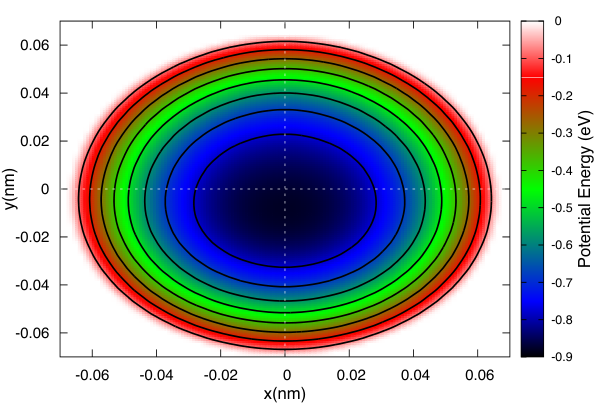

Using this model of a ground state wave function, we numerically estimate the hopping amplitude by integrating the product of two neighboring well ground state wave functions multiplied by the DFT potential over a circular region of radius centered on one of the two sites. At the same time, we can estimate the overlap integral for the wave functions of hydrogen states residing on adjacent atoms: , which plays a determinant role in the evaluation of the transition rate. Using the same model for the ground state wave function as above, numerical integration gives . This approximation of is an underestimate by construction of the model ground state wave function, as it ignores the other wells in the lattice. However, the small values of both and are reflecting the sharply localized nature of the hydrogen wave functions illustrated in Fig. 3, a posteriori justifying the approximation made.
A single hydrogen atom hopping over an ideal graphene sheet must therefore behave like a band particle and propagate with the band velocity . This velocity is much smaller than the band velocity of -electrons, m/s. Nonetheless, if hydrogen atoms absorbed by graphene were moving with such velocity , this would result in a rather quick homogenization of their distribution.
However, such a small (by microscopic scales) velocity means that the hydrogen bandwidth is very narrow. This should cause the suppression of elastic hopping as soon as the on-site potential energies between neighboring sites are different by more than . This is why the interaction mediated by conduction electrons makes elastic hopping impossible. When one of the atoms hops, it virtually always changes the sublattice, or : the likelihood of tunneling to a second-nearest neighbor on the same sublattice site is negligible, because of the much larger distance that must be covered. Suppose now that a second hydrogen atom happens to be some distance away, sitting atop a carbon atom belonging to the same sublattice. The interaction between the atoms then results in a positive energy . When one of the atoms hops to its nearest neighbor carbon atom, it lands on the opposite sublattice, and the interaction energy in the final state is negative, . The total energy change in this process, , therefore, exceeds both and . Even for two atoms sitting as far as a thousand interatomic distances apart, the energy change is estimated from Eqs. (1)-(2) to be of the order of . This energy is many orders of magnitude greater than the hydrogen adatom hopping bandwidth. We conclude, therefore, that the interaction mediated by conduction electrons makes elastic hopping impossible and results in a collective pinning of hydrogen on graphene.
Consequently, the tunneling can occur only if facilitated by additional processes which supply (or carry away) the energy difference. Such processes must involve excitations of graphene, phonons or electron-hole pairs. The transition rates in both cases are evaluated in Sections III and IV, respectively.
III Hydrogen-phonon interaction
Let us consider inelastic tunneling of a hydrogen atom between adjacent sites and where the atom has potential energy and , respectively. The extra energy , depending on its sign, must be carried away or supplied by phonons.
There are three low-energy phonon modes in graphene: longitudinal, transverse, and flexural. In the long wavelength limit, the first two have the usual acoustic dispersion, , while the third one has a quadratic dispersion. For the same frequency, long-wavelength flexural phonon modes have a much larger wave-vector and, accordingly, reside in a much larger phase space. We expect flexural modes to dominate phonon-assisted processes, similarly to how they dominate the phonon resistivity in electron transport[44].
The flexural phonon’s quadratic spectrum follows from the Hamiltonian for the out-of-plane sheet oscillations, which, in the long-wavelength limit, is[45]
| (5) |
with and denoting the two-dimensional mass density and the flexural rigidity constant of graphene, respectively. The Hamiltonian (5) describes unstrained graphene. In the presence of strain the Laplacian in is replaced with , in which case assumes the form of the usual membrane Hamiltonian. Below, we consider an unstrained sheet. As follows from the Hamiltonian (5), the spectrum of flexural modes is
| (6) |
Standard quantization of the Hamiltonian (5) leads to the following expression for the phonon flexural disturbance
| (7) |
in terms of the phonon creation and annihilation operators; stands for the normalization area of the sheet.
The hydrogen adatom represents a mass defect stuck to the graphene lattice. The coupling of the atom to the phonon field (7) is described by the additional kinetic energy of the atom’s oscillatory motion induced by the phonons,
| (8) |
Substitution of the phonon operator (7) into this expression yields the hydrogen-phonon coupling Hamiltonian
| (9) |
which consists of three terms. The first term describes absorption of two phonons with wave-vectors and ,
| (10) |
where . The second term is the Hermitian conjugate to the first one,
| (11) |
and describes the emission of two phonons. Finally, the term
| (12) |
describes scattering processes, in which a phonon with wave-vector is absorbed and a phonon with wave-vector is emitted.
In what follows we are going to utilize the perturbation theory to take into account the hydrogen-phonon coupling (9). Such approach is justified because of the light mass of hydrogen , which ensures that the coupling is going to be rather weak.
The probability of phonon-assisted hydrogen hopping from site to site follows from the Golden rule. For example, when hopping occurs with a decrease of the on-site energy, , only phonon emission and scattering processes are allowed. The transition rate for the emission is
| (13) |
From the Hamiltonian (11), we obtain that the matrix element for the emission transition is
| (14) |
where is the Bose-Einstein distribution with .
The total emission rate is found from Eqs. (13)-(14) by integrating over all phonon momenta. After simple calculation one finds,
| (15) |
Similarly, the probability of hydrogen atom hopping assisted by the absorption of a phonon with frequency and emission of a phonon with the higher frequency is given by
| (16) |
The transition rates (15) and (16) can be easily calculated in the limits of low and high temperatures. It turns out that the scattering channel is the dominant mechanism of phonon-assisted hopping when temperatures are high. On the other hand, emission prevails at low temperatures. This is expected since the number of phonons available for scattering is small in that case.
III.1 High temperatures,
In this limit, the denominators in the emission probability (15) can be expanded to the linear order in small . In the scattering probability (16) one may set since typical phonons participating in the process have much higher frequency, . Using the identity, , we obtain,
| (17) |
As mentioned above, at high temperatures the scattering-assisted processes are much more efficient in facilitating tunneling than the emission transitions. The -dependence of the scattering-assisted probability can be understood as follows. Phonons involved in the transition have energy of the order . One power of temperature arises from the number of such phonons available. The other two powers appear due to the fact that high-frequency phonons interact stronger with a hydrogen adatom, since they result in a larger coupling Hamiltonian (8).
III.2 Low temperatures,
In this limit, all exponentials with negative arguments can be discarded in both Eqs. (15) and (16). Additionally, since in the scattering channel the incident phonons have frequency , one may neglect in the numerator of the integrand of Eq. (16). Using the fact that , we find,
| (18) |
The predominance of emission over scattering in the low-temperature limit is driven by the scarcity of phonons in the initial state.
III.3 Hopping with the increase in energy,
When a hydrogen atom tunnels from a site with a lower interaction energy to a site with a higher energy it needs to pick up the extra energy to do so. This is possible by either absorbtion of two phonons via the process described by the Hamiltonian (10) or via the scattering processes already discussed above. The corresponding rates can be calculated from the same Golden rule formalism. However, they also follow immediately from the detailed balance principle, which provides,
| (19) |
At high temperatures, , therefore, the transition rates for the upward (in energy) tunneling are virtually the same as for the downward transitions. At low temperatures, , however, the upward transitions are strongly suppressed.
IV Hydrogen-electron interaction
Inelastic tunneling of a hydrogen atom can also occur with the excess (or deficit of) energy transferred to (from) the conduction electrons. At low energies, the latter have the Dirac spectrum .
The amplitude of this process is proportional to the matrix element of the interaction of a hydrogen atom with the electric charge of a conduction electron. A hydrogen adatom may interact with conduction electrons via Coulomb forces. Since the adatom is neutral, this interaction, in the lowest order, results from the dipole moment associated with the carbon-hydrogen bond and has the form,
| (20) |
where is the coordinate of the electron and is the adatom’s in-plane dipole moment. The coefficient is the effective dielectric constant of graphene, which describes screening of static electric fields by other conduction electrons.
From symmetry considerations, however, it is clear that the average dipole moment will be pointed in the direction perpendicular to the plane of graphene and thus the expectation value of the Hamiltonian (20) in the ground state of a hydrogen adatom is zero, . As long as there is no spontaneous symmetry breaking, we need to explore the second order correction.
This second order correction is analogous to the van der Waals interaction between two atoms where the interaction arises as a result of quantum fluctuations. The main difference comes from the fact that in our situation one of the particles (the electron) has a net charge, so that the resulting interaction falls of as , rather than as . Indeed, the second order energy correction is finite and given by the standard expression,
| (21) |
where the summation is taken over all excited states .
The actual energy levels and dipole moment’s matrix elements for a hydrogen atom sitting above a carbon atom in a graphene crystal can only be determined by first-principles calculations which are beyond the scope of the present paper. However, it is not difficult to estimate the correction (21) by the order of magnitude. The non-diagonal matrix elements are , where is the Bohr radius. Similarly, the difference is of the order of the Rydberg energy, . As a result, , which should be identified with the effective hydrogen-electron coupling energy, is,
| (22) |
where is an unknown positive dimensionless constant.
Expression (22) can also be obtained by purely classical considerations. The electric field produced by the conduction electron, and acting on the hydrogen atom, is ; for simplicity we set . This field is times weaker than the typical atomic fields, . It, therefore, leads to the displacement of the atomic electron of the order, , resulting in the induced dipole moment , from which Eq. (22) follows. Note that, for a free hydrogen atom, the dimensionless constant is known exactly[46], , suggesting that when the atom is sitting atop a graphene sheet.
We can now write the hydrogen-electron interaction (22) in the second-quantized form with the help of the electron creation and annihilation operators,
| (23) |
In this expression the indices and assume two values: for electrons in the upper Dirac cone and in the lower cone; the trigonometric factor in the brackets of the second line is coming from the pseudospin projection of the initial electron state onto the final state .
The Fourier transform of the interaction potential diverges at low distances and should be cut-off there by the Bohr radius,
| (24) |
The interaction is essentially short-range with the strength independent of the electron momenta. This is the result of the fast decay of the interaction (22) with the distance and the fact that only long-wavelength electrons, , can participate in the interactions, since energy involved in inelastic tunneling processes, , is small compared with the electron bandwidth.
The rate of inelastic tunneling transitions facilitated by the electron scattering is given by the Golden rule formula with the matrix element provided by Eq. (23):
| (25) |
where is the Fermi-Dirac distribution of electrons in the two cones. The overall coefficient in Eq. (25) takes into account the existence of two Dirac cones as well as the two-fold spin degeneracy. Note that yields the factor upon the angle averaging.
At high temperatures, , the main contribution comes from transitions that occur within the same cone, . In this limit can be neglected. After a simple integration we obtain,
| (26) |
At low temperatures, , the dominant process results from the lifting of an electron from the lower cone, , into the upper cone, , yielding the following inelastic tunneling rate,
| (27) |
Comparing these results with the rates for phonon-assisted tunneling from Section III, we see that the electron mechanism leads to the same temperature dependence as the dominant phonon processes: phonon scattering at high temperatures, see Eq. (17), and phonon emission at low temperatures, see Eq. (18). The reason for this coincidence is not difficult to understand. For example, at high temperatures electrons participating in the tunneling are confined in a smaller region of phase space; however, their coupling to hydrogen is stronger, since the coupling Hamiltonian (23) remains constant in the long-wavelength limit while coupling to phonons, Eq. (12), vanishes there.
V Discussion
Because of the similar temperature dependence, the ratio of the two rates takes a rather simple form. Interestingly, the two mechanisms appear to lead to rates of the same order of magnitude. At high temperatures, , the ratio of the two rates can be written as
| (28) |
The first ratio in this expression is , given the well-known value of the effective dielectric constant in graphene[45], , and the Fermi velocity, m/s. The second ratio is of the same order, , and is easily calculated from the value of the lattice spacing, nm, and the fact that the graphene lattice is honeycomb. Given the generally quoted value for the flexural rigidity constant[47] , the last ratio is very small, . However, this smallness is compensated by the large value of the numerical prefactor in Eq. (28). The constant is not known. However, if we utilize its value for a free hydrogen atom in the ground state[46], , we obtain that the ratio of the electron to the phonon contributions is
| (29) |
At low temperatures, , the ratio is given by the expression similar to Eq. (28) where there is an additional coefficient , as follows from Eq. (27) and the first line of Eq. (18). As a result, we have there.
The rates for inelastic hydrogen tunneling obtained in the preceding sections are rather small, predicting a very slow diffusion of hydrogen. Let us estimate the rate of hydrogen hopping in the dominant regime. Namely, consider the case of high temperatures where the scattering channel dominates, and the transition rate is given by the second line of Eq. (17). Using again[47] , and the overlap integral calculated earlier, , we find that in the high temperature limit the total hopping rate provided by the electron-assisted and phonon scattering rates is in terms of the reference temperature .
It is also instructive to restate the hopping rate in terms of the diffusion coefficient . To estimate its order of magnitude we assume that exceeds on each site, so that the probability of tunneling is uniform across the extent of the entire graphene sheet and is set by the temperature . The diffusion coefficient for a particle hopping on a honeycomb lattice with a given probability is then,
| (30) |
At room temperature the diffusion coefficient is of the order m2/s. Given this value of the diffusion constant, it would take a hydrogen atom a time years to diffuse across a micron-sized graphene flake.
In this paper we disregarded polaronic effect. The latter could be expected to renormalize mobility of a moving particle, by some numerical factor. On the other hand, the suppression of diffusion due to the effective interaction studied here appears to be a much stronger effect, by orders of magnitude.
Because of the slow character of hydrogen adatom diffusion, hydrogen desorption and absorption might become important in specific situations. Those processes depend on the ambient conditions and are beyond the scope of this paper.
VI Summary
For electronics applications utilizing graphene samples doped with resonant adatoms, such as hydrogen, it is important to predict how fast the adatom diffusion would occur at room temperatures. Fast diffusion could be favorable for the device manufacturing, but it would be detrimental for the device longevity. On the other hand, fast diffusion would be required for the realization of various phases resulting from adatom ordering[48, 49, 50].
Our calculations show that the diffusion of hydrogen adatoms, the lightest dopants, is very slow. A single adatom placed on an ideal graphene sheet would propagate with the velocity of the order of 1 cm/s. However, the presence of other such adatoms suppresses adatom propagation dramatically. This is the result of a peculiar electron-mediated effective interaction between adatoms. Two features make this interaction efficient in suppressing diffusion. First, it is a is long-range interaction, so that it is considerable even when adatoms are tens of nanometers away from each other. Second, it changes sign depending on whether adatoms reside on the same or opposite sublattices. In order to move, an adatom would have to hop to a nearest neighbor carbon site and change its energy in the process by as much as tens of meV. Such inelastic hopping requires assistance from phonons or electron-hole excitations.
Let us emphasize that the suppression of the diffusion discussed in this paper is due to the graphene band structure featuring two Dirac points, which results in a quantum interference of the electron band states propagating over two sublattices in the honeycomb arrangement of carbon atoms. The effective hydrogen-hydrogen interaction, which has opposite sign on the two sublattices, originates from coupling of hydrogen adatoms to such band electrons.
As a result, we find a single adatom hopping time to be in the range of milliseconds at room temperature. This indicates that the diffusion is sufficiently slow that hydrogen-doped graphene devices are feasible. However, it is too slow for any gate-control of the hydrogen adatom distribution to be useable in fast switching devices.
Acknowledgements.
We thank Oleg Starykh and Janvida Rou for helpful discussions. S.L. and J.T. acknowledge the support by NSF through MRSEC DMR-1121252. E.M. was supported by the Department of Energy, Office of Basic Energy Sciences, Grant No. DE-FG02-06ER46313.References
- [1] A. H. Castro Neto, F. Guinea, N. M. R. Peres, K. S. Novoselov, and A. K. Geim, Rev. Mod. Phys. 81, 109 (2009)
- [2] V. V. Cheianov and V. I. Fal’ko, Phys. Rev. Lett. 97, 226801 (2006).
- [3] A. B. Kuzmenko, I. Crassee, D. van der Marel, P. Blake, and K. S. Novoselov, Phys. Rev. B 80, 165406 (2009).
- [4] Y. Zhang, T.-T. Tang, C. Girit, Z. Hao, M. C. Martin, A. Zettl, M.F. Crommie, Y. R. Shen, and F. Wang, Nature 459, 820 (2009).
- [5] K. F. Mak, C. H. Lui, J. Shan, and T. F. Heinz, Phys. Rev. Lett. 102, 256405 (2009).
- [6] G. Giovannetti, P. A. Khomyakov, G. Brocks, P. J. Kelly, and J. van den Brink, Phys. Rev. B 76, 073103 (2007).
- [7] Z. H. Ni, H. M. Wang, Y. Ma, J. Kasim, Y. H. Wu, and Z. X. Shen, ACS Nano 2, 1033 (2008).
- [8] Z. H. Ni, T. Yu, Y. H. Lu, Y. Y. Wang, Y. P. Feng, and Z. X. Shen, ACS Nano 2, 2301 (2008).
- [9] P. Shemella and S. K. Nayak, Appl. Phys. Lett. 94, 032101 (2009).
- [10] K. S. Kim, Y. Zhao, H. Jang, S. Y. Lee, J. M. Kim, K. S. Kim, J. H. Ahn, P. Kim, J. Y. Choi, and B. H. Hong, Nature (London) 457, 706 (2009).
- [11] V. M. Pereira, A. H. Castro Neto, and N. M. R. Peres, Phys. Rev. B 80, 045401 (2009).
- [12] G. Cocco, E. Cadelano, and L. Colombo, Phys. Rev. B 81, 241412(R) (2010).
- [13] M. Ezawa, Phys. Rev. B 73, 045432 (2006).
- [14] Y.-W. Son, M. L. Cohen, and S. G. Louie, Phys. Rev. Lett. 97, 216803 (2006).
- [15] M. Y. Han, B. Özyilmaz, Y. Zhang, and P. Kim, Phys. Rev. Lett. 98, 206805 (2007).
- [16] C. L. Kane and E. J. Mele, Phys. Rev. Lett. 95, 146802 (2005).
- [17] Zh. Qiao, Sh. A. Yang, W. Feng, W.-K. Tse, J. Ding, Y. Yao, J. Wang, and Q. Niu, Phys. Rev. B 82, 161414(R) (2010).
- [18] C. Weeks, J. Hu, J. Alicea, M. Franz, and R. Wu, Phys. Rev. X 1, 021001 (2011).
- [19] A. Bostwick, J. L. McChesney, K. V. Emtsev, T. Seyller, K. Horn, S. D. Kevan, and E. Rotenberg, Phys. Rev. Lett. 103, 056404 (2009).
- [20] D. C. Elias, R. R. Nair, T. M. G. Mohiuddin, S. V. Morozov, P. Blake, M. P. Halsall, A. C. Ferrari, D. W. Boukhvalov, M. I. Katsnelson, A. K. Geim, K. S. Novoselov, Science 323, 610 (2009).
- [21] R. Balog, B. Jørgensen, L. Nilsson, M. Andersen, E. Rienks, M. Bianchi, M. Fanetti, E. Løgsgaard, A. Baraldi, S. Lizzit, Z. Sljivancanin, F. Besenbacher, B. Hammer, T. G. Pedersen, P. Hofmann, and L. Hornek, Nature (London) 9, 315 (2010).
- [22] J. Ding, Zh. Qiao, W. Feng, Y. Yao, and Q. Niu, Phys. Rev. B 84, 195444 (2011).
- [23] J. O. Sofo, A. S. Chaudhari, and G. D. Barber, Phys. Rev. B 75, 153401 (2007).
- [24] T. O. Wehling, M. I. Katsnelson, A. I. Lichtenstein, Chem. Phys. Lett 476, 125 (2009).
- [25] V. Mostepanenko and N. Trunov, The Casimir Effect and Its Applications (Clarendon, Oxford, 1997).
- [26] A. V. Shytov, D. A. Abanin, and L. S. Levitov, Phys. Rev. Lett. 103, 016806 (2009).
- [27] S. LeBohec, J. Talbot, and E. G. Mishchenko, Phys. Rev. B 89, 045433 (2014).
- [28] S. Casolo, O. M. Lovvik, R. Martinazzo, and G. F. Tantardini, J. Chem. Phys. 130, 054704 (2009).
- [29] Z. Sljivancanin, E. Rauls, L. Hornekaer, W. Xu, F. Besenbacher, and B. Hammer, J. Chem. Phys. 131, 084706 (2009).
- [30] Y. Ferro, F. Marinelli, and A. Allouche, Chem. Phys. Lett. 368, 609 (2003).
- [31] Y. Ferro, F. Marinelli, A. Jelea, and A. Allouche, J. Chem. Phys. 120, 11882 (2004).
- [32] L. Hornekær, E. Rauls, W. Xu, Ž. Šljivančanin, R. Otero, I. Stensgaard, E. Lægsgaard, B. Hammer, and F. Besenbacher, Phys. Rev. Lett. 97, 186102 (2006)
- [33] L. Chen, A. C. Cooper, G. P. Pez, and H. Cheng, J. Phys. Chem. C 111, 18995 (2007).
- [34] Y. Lei, S. A. Shevlin, W. Zhu, and Zh. X. Guo, Phys. Rev. B 77, 134114 (2008).
- [35] T. O. Wehling, M. I. Katsnelson, and A. I. Lichtenstein, Phys. Rev. B80, 085428 (2009).
- [36] D. W. Boukhvalov, Phys. Chem. Chem. Phys. 12, 15367 (2010).
- [37] H. McKay, D. J. Wales, S. J. Jenkins, J. A. Verges, and P.L. de Andres, Phys. Rev. B81, 075425 (2010).
- [38] L.F. Huang, M. Y. Ni, X. H. Zheng, W. H. Zhou, Y. G. Li, and Z. Zeng, J. Phys. Chem. C 114, 22636 (2010).
- [39] V. A. Borodin, T. T. Vehviläinen, M. G. Ganchenkova, and R. M. Nieminen, ”Hydrogen transport on graphene: Competition of mobility and desorption”, Phys. Rev. B 84, 075486, (2011)
- [40] Y. Wang, H.J. Qian, K. Morokuma, S. Irle. J. Phys. Chem. A. 116, 7154 (2012).
- [41] Y. Shao et al,Mol. Phys. 113, 184 (2015).
- [42] C. C. Marston, G. G. Balint-Kurti. J. Chem. Phys. 91, 3571 (1989).
- [43] A. Stathopoulos, J.R. McCompbs. ACM Transaction of Mathematical Software. 37, 21:1 (2010).
- [44] E. Mariani and F. von Oppen, Phys. Rev. Lett. 100, 076801 (2008).
- [45] A. H. Castro Neto, F. Guinea, N. M. R. Peres, K. S. Novoselov, and A. K. Geim, Rev. Mod. Phys. 81, 109 (2009).
- [46] L. D. Landau and E. M. Lifshitz, Quantum Mechanics: Non-Relativistic Theory, (Addison-Wesley, Reading, Mass., Oxford, 1958).
- [47] N. Lindahl, D. Midtvedt, J. Svensson, O. A. Nerushev, N. Lindvall, A. Isacsson, and E. E. B. Campbell, Nano Lett. 12, 3526 (2012).
- [48] V. V. Cheianov, O. Syljuasen, B. L. Altshuler, and V.I. Falko, Europhys. Lett. 89, 56003 (2010).
- [49] D. A. Abanin, A. V. Shytov, and L. S. Levitov, Phys. Rev. Lett. 105, 086802 (2010).
- [50] S. Kopylov, V. Cheianov, B. L. Altshuler, and V.I. Fal’ko, Phys. Rev. B 83, 201401(R) (2011).