Super-Languages
Developing Languages and Applications with XMF
Second Edition
![[Uncaptioned image]](1506.03363v1/SuperXMF.png)
Tony Clark, Paul Sammut, James Willans
Chapter 0 Introduction
The days of monolithic languages are over. The idea that one size fits all is dead. Long live diversity!
Applications should not, and indeed cannot, be written in a single language these days. We have lots of technologies that are specific to different aspects of complete application. We have SQL for databases, we have JSP for web presentation, we have XML everywhere, we have Java and J2EE, we have frameworks and libraries. So everything is great - just map you application to an appropriate technology and away you go!
But wait a minute, perhaps this diversity is not such a good thing. Representing our application in these technologies can be quite hard. I understand how the application breaks down into aspects, but those aspects don’t seem to map down onto different aspects of the technology very well. OK, so, I’ll put a bit of each application feature into the appropriate technologies. It takes a bit of translation, but our guys are experts in the technologies so there should be no problem. Great - the system works, everyone is happy.
Uh, oh - the requirements have changed. No matter - we’ll just talk it through with the customer and modify the implementation accordingly. It will take a bit of time to trace the requirements through to the implementation on all those different bits of technology, er how did we implement that customer transaction again? Never mind, we can put that other project on hold while the original developers are brought back to reverse engineer the code.
Yikes! the original developers have left. Just great, now I have to pick through all those technologies and try to do it myself. Crikey - I don’t really understand this stuff, it talks about accrual periods and debentures. I know, I’ll show it to the customer, surely they can extract some meaning from this mess. Aargh - the customer won’t touch it and the new development team just wants to rewrite it!
1 The Representation Chasm
We are drowning in implementation technology. Software language engineers have been very busy over the last 10 years inventing languages that control the new frontiers of technology. In particular there are a huge number of languages that provide control over distributed applications, databases and web-content. Basic technology issues are very well provided for. This can be seen in the rise of open-source technologies and the standardisation of architectures for information processing applications.
And yet there are still problems. Little attention has been paid to closing the gap between the languages and the applications that they implement: the representation chasm. The chasm is bridged by highly skilled developers who take designs and produce the application. But what if your developers are not as highly skilled as you would like? This leads to errors and delays arising from misunderstandings. Iterative development is compromised by the representation chasm since various project stakeholders become disenfranchised depending on which side of the chasm they live. Maintenance become difficult: the customers, architects and designers shout new requirements from one side of the chasm only for the development team to mis-hear them on the other.
How do we bridge the representation chasm? The answer is in moving towards a new breed of language technology: super-languages. A super-language provides a number of technical features that are specifically designed to close the gap between the concepts in the application domain and the technologies that are used to implement the application. Super-languages can be used to empower development teams by increasing the sophistication of the tools they use to implement the application.
Super-languages can be used to de-skill various aspects of the implementation by offering restricted languages suitable for the application. Super-languages can be made accessible to project stakeholders that would usually be unable to engage with implementation technologies. Super-languages can radically increase the efficiency of the development team and can radically increase the quality of the delivered products, derisk the development process, and increase the ability of the supplier to maintain the products.
2 Super-Languages
What is a super-language and how does it differ from the current breed of implementation technologies? An idealised super-language provides control over all aspects of representation and execution. A super-language can be extended with new features that make it easy to represent concepts from the application that a customer would understand. These new concepts can be weaved into the existing features of a super-language or may be kept separate (as a different aspect for example). Existing execution mechanisms in the super-language can be changed to reflect the needs of each new application. Each new feature that is added to a super-language has a description of how it should execute and how it integrates with other features (where that is appropriate).
A super-language must provide super-features that address: usability; expressiveness; extensibility. These are described in more detail in the following sections.
1 Usability
A super-language must be fit for purpose. It should support the developer in capturing features of the application and place no unnecessary barriers in the way of development. The following features contribute to the usability of a super-language:
- interactive
-
A super-language cannot be a batch execution language. Some form of top-level command interpreter is essential. Developers want to interact with their programs and to deny them this pleasure is cruel. Interactivity aids development and debugging, increases developer productivity, and facilitates a deep understanding of execution mechanisms. If a super-language is used for language engineering then the developer will be implementing execution mechanisms which will require a good understanding of how languages tick.
- dynamic
-
A super-language must be dynamic. It must be possible to load new definitions into the language at any stage during execution. Why wait to recompile and restart an application when it is not necessary? A super-language may be used as the glue that binds an application made up of many different modules written in a variety of languages. In order to be glue, the super-language must provide mechanisms for dynamically loading and processing the modules. This is closely related to the idea of aspects.
- reflection
-
A super-language must be able to reflect on its own structure and behaviour. It should be possible for the language to query its own state and to represent and manipulate its own syntax. Many of the domain specific languages that are represented by super-languages will ultimately be represented in a basic core language (an alternative is to be translated to some external language). Syntax translations rely on having a complete representation of the super-language syntax available to the language engineer.
- interfaces
-
Super-languages must not be closed worlds. It is unrealistic to expect mainstream programming languages to become super-languages overnight. In addition there are practical reasons why certain aspects of a system may need to be implemented using conventional technology. Therefore, until standard languages become super-languages, a super-language should support interfaces to conventional technology. Super-languages should support provision for running as embedded applications.
2 Expressiveness
Where possible, a super-language should abstract away from implementation details in programs. It should be possible to quickly and efficiently use a super-language for prototyping an application in addition to product development. Key features are:
- high-level
-
There is no excuse for a language which does not provide features that make representation and computation easy to achieve. These include things like heterogeneous lists; closures; pattern matching; symbolic data; rich type systems etc. High-level features make a language a pleasure to use and contribute to the readability of the code. Closures are particularly important since they can be used to engineer applications that would be complex and difficult to understand without them (particularly search related applications).
- dynamic(duck)typing
-
Languages that are limited to static type systems are too restrictive to be super-languages. It is difficult to achieve interaction and meta-features with exclusively statically typed languages. Trust the developer - they really do know what they are doing! The type-system of a super-language should be extensible just like all other aspects of the language. A super-language may optionally impose static typing (static typing is a good thing), but should not mandate it.
- garbage-collection
-
The days of direct pointer manipulation and user defined memory management are surely behind us. All but the very specialized real-time or hardware related applications cannot justify the exposure of raw machine-level details in this way.
3 Extensibility
A super-language must be extensible. In principle, all aspects of the language from the syntax to the execution engine should be available to the developer. Extensibility features must be fullsome and integrated with the rest ofthe language. It does not count if you provide a couple of system calls that changes the mode of the execution engine. It does count if you can write a complete new execution algorithm and plug it in. It does not count if you write a pre-processor for your language. It does count if you can write a source code translator and integrate it into the language compiler using all of the context that the compiler manipulates. Key features are:
- aspects
-
A super-language must support the idea of aspects whereby new definitions can be added to existing language components. Ideally the super-language will be written in itself and must be extensible so that it can be tailored through extension to suit different application domains. Groups of definitions added to existing components are grouped into logically related packages or aspects. It should be possible to manipulate aspects as a unit, minimally in terms of addition, deletion and debugging.
- reflexive
-
A super-language should be reflexive. This is related to reflection, but differs in that the language can affect its own behaviour. Debuggers for languages rely on the ability to be reflexive since they have to change the trace state of the operations that they are tracing. An ideal super-language will be meta-circular since this is the best way of ensuring (given the characteristic features listed here) that the language will be sufficiently expressive.
- meta-protocols
-
Execution engines for languages are like software frameworks. To plug into the framework you supply program code written in a language that the framework understands. The framework executes and processes the program code. The key steps in execution forms an execution procotol for the framework. The execution protocol for a super-language must be clearly defined. A meta-protocol is a collection of features that can be used to extend or redefine the execution protocol. A super-language should offer a meta-protocol that allows new languages to hook into the existing execution framework, but which allows them to change it. A typical excample is the protocol for an object-oriented language that includes: send; setSlot; getSlot etc. A meta-object-protocol (or MOP) allows you to replace the definition of these features for specific types of object.
- lightweight-extensible-syntax
-
The syntax of a super-language must be extensible and ultimately replaceable. In order to be a power-tool for developers, the super-language must allow new language features to be added and weaved into the existing language. New language features must be able to take full advantage of the execution framework for the super-language including accesing context information such as local variables etc. Super-languages should support the definition of new language features that support standard programming idioms and also support the publication of such definitions for others to reuse.
- heavyweight-extensible-syntax
-
A super-language should provide features that support the definition of complete external languages. Such language should support a development method that allows different aspects of a system to be represented by DSLs that are accessible to external stakeholders and which may also deskill the development process. These languages are not necessarily weaved into the main super-language, instead they are used externally to the main language and loaded on demand.
3 The Pros and Cons of Super-Languages
The benefits of super-languages have been outlined above. They empower the developer to be more productive by raising the abstraction level of the programming language and inventing standard representations for common idioms. This technique has been used in many programming languages from the C-preprocessor through to Lisp. New language constructs can be standardized and shared.
Super-languages also provide an unprecedented degree of control over the language engine via meta-features. Access to meta-features provides a way of tailoring a language in a modular way without polluting programs. This separation of concerns is very powerful and can be used to support a mixed paradigm application on the same language platform without compromising the readability or maintainability of the application.
If used to implement multiple heavyweight or external languages within the same application, super-languages provide the basis for addressing some of the significant concerns raised at the beginning of the chapter relating to current implementation technology and the representation chasm. This can lead to significant commercial benefits arising from the ability to engage more stakeholders will all aspects of an application and the ability to control and deskill aspects of the application development.
Super-languages are not without their problems. Since they offer advanced features they can be used inappropriately and can be challenging for the novice programmer. The techniques used to implement super-languages are not as mature as those for more conventional languages and therefore efficiency and useability issues can be an issue. It is important to put these issues in perspective. Super-languages represent a technology goal for current generation programming languages to aim for. The software industry must embrace super-languages and help to develop the technologies and methods since they represent a very significant step forward in software application development. Existing mainstream languages should strive to adopt super-features and thereby move forward.
4 Related Concepts
The concept of super-languages is related to several other terms used by the software industry. These are:
- LOP
-
Language Oriented Programming is a term that is used to mean the process of defining new programming concepts in order to address a given application. A super-language supports LOP although not all systems that support LOP need be super-languages. It is not necessary to be a programming language in the first place to support LOP - you just need to be a system that allows the definition of programming languages. It is certainly not necessary to be meta-circular to provide LOP.
- DSL
-
Domain Specific Languages is a term that is used to mean a language that has been specifically designed to represent concepts from an application domain. A super-language supports DSLs, however the term DSL can mean languages that do not involve programming in any way. The term includes graphical languages, such as profiles in UML, that are used to express designs in terms of concepts and relationships.
- LDD
-
Language Driven Development is a method that can be used to produce software applications. LDD involves the use of DSLs at various points in the development life-cycle. If LDD is used as part of the implementation phase of the project then the use of super-languages is almost essential.
- MDA
-
Model Driven Architecture is a term used to mean the generation of program code from UML models, possibly involving the use of DSLs or UML profiles. Super-languages are not specifically required for this process (although they may help in the transformation process - see QVT).
- Software-Factories
-
Software factories is a term used to mean the application of standard industry practices to software development. More specifically it has been used to refer to an approach supported by Visual Studio to develop languages that support the construction of software components. This is similar in many ways to MDA, but is not limited to using UML.
- Language-Workbenches
-
The term language workbench was proposed by Martin Fowler in http://martinfowler.com/articles/languageWorkbench.html to mean the IDE support for language oriented programming. Examples of language workbenches include Intentional Software, the Meta programming System from JetBrains and the Visual Studio provision for Software Factories. A super-language is not an IDE. Programming and development processes that are based on super-languages do not require IDE support. However, given that super-languages are by nature more sophisticated than conventional languages, IDE support and language workbenches are an important tool.
5 Examples of Super-Languages
The perfect super-language does not exist. Such a language would be arbitrarily extensible, as efficient and usable as current languages, have IDE support for all aspects of the language and would integrate with anything. The perfect super-language is an ideal that should motivate current language developers to strive for better features that can address the representation chasm.
Languages with super-features do exist and have done so for quite a while. Smalltalk and Lisp offer a significant number of super-features although both frighten the horses in terms of scary syntax.
C# and Java offer a degree of reflection, but offer no support for language extension and high-level programming features. It would be very interesting to chart out a course of language evolution for these languages which incrementally adds super-features.
Languages such as Ruby and Python offer a range of super-features, including dynamic typing and meta-features, but are generally fixed in their syntax. It is interesting to note that this style of language (often referred to as scripting languages) are generally popular with technology lead programmers. This is a good indicator that languages with super-features are likely to find their way into the mainstream.
6 The Super-language XMF
This book is about a language system called XMF. XMF has been designed as a super-language and offers a full range of super-features. XMF is not the perfect super-language, but it claims to be the language that exhibits more super-features than any other language currently available. XMF has been in development since around 2000 and has gone through a number of development cycles. Its roots are in the Object Management Group initiative to define the UML 2.0 standard when an early version of XMF was developed in order to process fragments of UML language definition. In case anyone is wondering, this explains the terms OCL and XOCL that occur in XMF and also explains some of the syntax used in XMF. The relationship between XMF and UML/OCL was dropped many moons ago, leaving some of the features that contribute to being a super-language and dropping all others.
Since 2003, XMF has been actively developed as a commercial product and used by real paying customers as part of a larger product called XMF-Mosaic. The Mosaic component was a large library of XMF code (over 100K lines of XOCL) that implemented diagram tools and property editors generated from XMF meta-descriptions. Mosaic allowed XMF to run inside Eclipse. At the time, Mosaic was ahead of the game, but since we started development on Mosaic, systems like EMF/GMF and Software Factories have caught up and overtaken Mosaic in terms of development effort. In any case, Mosaic was a sophisticated working example of a fairly large XMF application and shook most of the bugs out of the system.
The key super-strengths of XMF:
- •
it is written in itself and therefore it is highly self consistent. Since extensibility is part of the language, this makes XMF completely extensible.
- •
it provides extensive support for working with syntax, both concrete and abstract. XMF is a true LOP engine.
- •
it provides very high-level programming features including pattern matching, undoability, daemons, heterogeneous lists.
- •
it implements a MOP and is truly meta-circular. The meta-language is called XCore which defines all the data types and behaviour for the rest of the system. There is no fudging of meta-classes as occurs in some language systems.
- •
it is interactive, dynamic and multi-threaded.
- •
it can be embedded in Java both calling out to Java and being called from Java.
The weaknesses of XMF as a super-language are:
- •
it is not as fast as a mainstream language. For many super-applications this will not be a problem.
- •
error handling is adequate, but no special support is provided for new languages engineered with XMF.
- •
there is no static typing (although this is planned for the next major release).
7 Guide to Book
The aim of this book is to introduce you to the super-language XMF. This will be done by defining the language, providing some examples of applications that can be written directly in the XOCL language that comes with XMF, and then by showing how you can use XMF for language engineering.
The main focus of this book is on language engineering by example. Although we introduce the XOCL language in general terms, we quickly focus on the features that make XMF good for writing new languages and then give lots of examples.
There are many super-features of XMF that we do not cover. These features include: Java interface; daemons; undo. We don’t spend very much time on the MOP and the meta-interfaces of XMF.
XMF is open-source technology. You can get a copy of XMF from www.ceteva.com. Since XMF is written in itself, it is one of the best examples of how to write XMF programs. In addition to the material in this book we would encourage you to check out the XMF source code for examples of how to write languages and how to program in XMF.
This book is divided into the following parts:
- XOCL
-
The XMF programming system consists of a language called XOCL that runs on the XMF VM. In order to program in the XMF system you will need to learn XOCL. This part includes a tutorial on XOCL and the main data that runs on the XMF VM.
- Programming
-
This part of the book describes a number of applications written in XOCL. None of the applications involve language engineering, just using XOCL to produce a program that runs on XMF.
- Language-Engineering
-
Super-languages allow new language constructs and even complete languages to be defined. This part of the book provides a number of examples of how you can use XMF to engineer languages.
8 References:
- •
http://www.cse.dmu.ac.uk/~mward/martin/papers/middle-out-t.pdf
- •
http://www.onboard.jetbrains.com/articles/04/10/lop/
- •
http://martinfowler.com/articles/languageWorkbench.html
- •
http://www.infoq.com/presentations/domain-specific-languages
- •
http://www.martinfowler.com/
Part 1 XMF
Chapter 1 Languages
In order for a language to be at all useful it must mean something. Meaning is a difficult thing to grasp since in order to talk about it at all it is necessary to use language which itself involves a question of meaning. However, it is possible to set down some broad ground-rules that can be used to establish a basic framework.
First of all, a language has a syntax which comes in two flavours: concrete and abstract. Concrete syntax is how you read or write a language, it tends to be human-centric. The following is an example of concrete syntax:
Abstract syntax deals with how a language is represented as data; it tends to be computer-centric. Here is the equivalent example represented as abstract syntax (think of the Java data structure that is created rather than the characters making up the program):
In order to build systems we need a language with a syntax. Rather than use any old language, this book is about constructing languages that are a good fit for the required system. In doing so we need control over the concrete syntax (to make it easy to work with for a human) and control over the abstract syntax (to make it easy for a computer to work with it).
The process by which concrete is turned into abstract syntax is called parsing. This book deals with models of languages and provides a great deal of examples of grammars that specify how to turn concrete into abstract syntax language representations.
Next, the syntax of a language does not define its meaning any more than you can judge a book by its cover. In order to have meaning, a language must have a semantic domain. A semantic domain is a model of the elements that the language denotes. A semantic domain for natural language (such as English) contains all the real-world concepts you can think of (such as Elephants and houses) in addition to all the conceptual things you can think of; in fact, it contains anything you can think of.
Languages used for system development are much more controlled in terms of syntax and semantics than natural languages. The semantic domains of such languages are defined by data types for elements appropriate to the systems domain. The particular data types depend on the system domain, for example a language for expressing telecomms will have a semantic domain containing networks, routers and devices. Languages defined for general use have general purpose semantic domains containing such things as records, integers, strings, events etc.
Finally, the meaning of a language is not defined by its syntax or its semantics alone; the meaning is the mapping that links the syntax to the semantics. In terms of modelling languages the mapping is often static, for example linking class definitions to sets of objects that are the instances of the classes. This of UML-style class models. What is the meaning of such a model? Since the class diagram does not specify any behaviour, neither does the semantics. a suitable semantics might be all the objects that can be constructed whose structure matches that specified in the class model. For programming languages the mapping is dynamic since it links programs to execution traces and all the execution machinery that lives in the traces.
To understand a language you must be fluent in its syntax, its semantic domain and the mapping between them.
This book defines the super-language XMF and describes how you use it to bridge the representation chasm. This book is not about how you analyse the systems themselves in order to model them; there are plenty of books about that topic. This book aims to provide a collection of techniques that allow you to raise the abstraction-bar when addressing system development issues.
When modelling systems it is desirable to focus on what is being expressed rather than how the information is being represented. This is the essence of a language driven approach: we can use high-level abstractions to capture the information without worrying about unnecessary implementation detail. The language that will be used to represent the information in this book is designed to provide a wide range of high-level constructs for modelling information.

Futhermore, the language has been specifically designed to be extensible: if no language construct is provided to express the required information then the user can extend the language with a new construct that does the job. This is the ball-of-mud model first pioneered by the Lisp family of programming languages. Rather than being a pejorative term, a language is like a ball of mud when new features can be added to the language in a way that the new features become part of the language and are indistinguishable from the existing features. No special actions need to be taken to use the new extensions: they have been seamlessly integrated into the language.
Rather than being a ball of mud, it is possible to view the different languages as towers as shown in figure 1. The base level is a very general language that supports the construction of other language (ideally it will support the definition of itself). A language is grown from the basic framework by adding successive layers of language constructs; each layer is built from all those layers below it and the layers become progressively more tailored to specific application domains. The ball of mud principle is maintained when the addition of a layer does not preclude the use of constructs from lower layers and when languages build in different towers can be used in the same application.
This chapter defines the semantic domain for the language that is used throughout the rest of the book. The next chapter describes the syntax of the language XOCL. The chapter after than describes language building features. On reading the rest of this chapter you should expect to appreciate the key data values that can be expressed and the kind of operations that are applied to the values. Each major category of value has a section to itself.
The element types are divided into groups described in the following sections. In each case the types that form a coherent aspect of the semantic domain are grouped together. An overview of the aspect is given along with a collection of operations that make up an interface for the group. Note that the interface is very general; it is intended that a given application will extend this interface by dynamically adding more operations to the domain types as required. In addition, the operations describes in each section are an overview. The gold standard of operations for each type is the source code of XMF itself.
1 Everything is an Element

Figure 2 shows the root class of the value domain: everything is an element - some things are objects. When designing the value domain we had a choice: should everything be an object? Objects have state represented as slots; a slot has a name and a value. The slots of an object can be updated. Objects have an identity: when you create an object it will be different to every other object that you have ever created (even if the slots are the same).
But not all values have changeable state and an identity. For example: the integer 3. Does it make sense to talk of the state of 3? Does it make sense to change the state of 3? Given two occurrences of 3, are they the same or not?
The distinction between Element and Object allows us to make the distinction between values whose state cannot change and which have no identity. Therefore, 3 is an element, but not an object. A set is an element and not an object, as is a string and a boolean value.
Our language is object-oriented and computation proceeds by message passing. When an element is sent a message, if its type defines an operation with the same name as the message then the operation defines the actions that are performed. If T defines an operation o expecting arguments (x,y,z) then T::o(x,y,z) is the operation. In the rest of this chapter each section defines some types; the key operations for the types are described; where the type of arguments or the return type of an operation is Element then the type is omitted.
The main operations defined by Element are:
The main operations defined by Object are:
2 Indexing Things

When dealing with values it is desirable to build collections where the elements in the collection are indexed by a key. The key is specified when the element is placed into the collection and the key is used to look the element up in the collection. The value associated with a key in a collection may be changed.
Figure 3 shows three classes that are used to represent basic indexed collections. Notice these classes extend Element, not Object, therefore these indexed collections have no slots. A table uses any element as a key, buffers and vectors use integers as keys. The difference between a buffer and a vector is that the former grows to accommodate elements as they are added whereas the latter is a fixed size.
What would you use these for? A table is useful when building arbitrary associations, for example associating names of personnel with their employment records. Vectors are useful when you know the size of the collection in advance, for example the locations on a chess board. Buffers are useful when you need the collection to grow as required and want to index elements by their position, for example building an output string.
The main table operations are as follows:
The main buffer operations are as follows:
The main vector operations are:
3 Naming Things and Looking Them Up

Elements are often identified by their name and the value domain provides special support for named elements and their containers. Figure 4 shows the classes that define these elements. A contained element has a link to its owner and a named element is a contained element with a name. A container is a class that wraps up internal storage implemented by tables, vectors and the like. An indexed container is a wrapper for a table (allowing users to extend the class). A name space is a named element that contains other named elements.
Notice that the structure of a name space allows name spaces to contain other name spaces. This means that references to named elements may cross a number of nested name spaces, leading to the idea of a path to an element. There is always a global name space called Root in the value domain: everything is contained in Root. A path is a sequence of names separated by ’::’. So Root::X references the named element with the name X in the name space Root. If X is a name space containing a named element Y then the path is Root::X::Y. Since Root is special, it can be omitted: X::Y.
The main operations defined by Contained are:
The main operations defined by Container are:
The main elements defined by NamedElement are:
The main operations defined by IndexedContainer are:
A package is a special type of name-space that contains operations, classes and sub-packages. Most of XMF is constructed around packages. When you write your own applications in XMF you will probably define one or more packages to contain the definitions.
4 Classifying Things

The values in a value domain fall into different groups: the integers, the objects, the personnel records, the update events etc. Each of these groups is a type and there is an element that represents the type: a classifier. A classifier is a single value that defines characterising features of a group of values: its instances. Each instance in the group refers to the classifier as its type. For example the integer 3 has Integer as its type. Furthermore, sub-groups can often be identified such that elements of a sub-group have more characterising features - this is specialization.
Figure 5 shows the classes that define classification. A classifier defines a collection of constraints: rules that govern the characterising features of its instances. A classifier has parents, the child parents are spcializations of the parent classifiers. All the constraint rules of the parents are used to classify the instances of the child classifier which may add rules of its own. Finally, a classifier has a default element, for example the classifier Integer has a default value of 0.
Classifier defines the following operations:
Each element in figure 5 is a classifier. For example NameSpace classifies all name spaces in the value domain such that a name space must have a collection of named elements and must itself be a named element. It is always possible to ask an element in the value domin what its classifier is. The operation Element::of() returns a classifier; since this is provided by Element which classifies everything, then all values in the domain support this operation.

The basic data values such as 10, true and “a string” are all classified by distinguished classifiers Integer, Boolean and string. These classifiers, in turn are classified by the classifier DataType as shown in figure 6. The special value null is classified by Null; it is used as the default value for all values that have internal state.
The types String, Integer, Float, Boolean and Null each define their own collection of operations that are listed in the appendix.
5 Collections of Things

Two types of non-indexed collections are very useful: sets and sequences. A set is an unordered collection, adding the same element to a set has no effect and it is not possible to rely on the order of elements in a set. The following is a set of integers: Set{1,2,3,4}, it is the same set as Set{4,3,2,1} and the set Set{1,1,3,2,3,4}. Figure 7 shows the classifiers that apply to sets and sequences. In general the classifier of a set of elements of type T is Set(T); since everything is classified by Element then the most general set-based classifier is Set(Element).

A (non fixed size) sequence is either empty Seq{} or is a value v followed by a sequence s: Seq{v — s}. A sequence has a head, v, and a tail, s. Sequences lend themselves to recursive processing by case analysis on the empty sequence and the non-empty sequence. Sequences of elements of type T are classified by type Seq(T) and the most general sequence classifier is Seq(Element).
Figure 8 shows the sequence Seq{1,2,3} which is equivalent to the sequence Seq{1 — Seq{2 — Seq{3 — Seq{}}}}. The head of the sequence is the integer 1 and the tail of the sequence is Seq{2,3}. The final dot in the figure represents the empty sequence Seq{}.
Sequences of element are used heavily in this book to represent collections. They are built-in to the implementation of the language and cannot be extended. The appendix lists many of the operations that are provided for manipulating sequences.
6 Classifying Objects

Objects are values with identity and state. The identity is set when the object is created and the state is represented as a collection of slots. Each slot has a name and a value. Objects are used to represent elements with properties, for example personnel records have personnel properties including the name of the employee, salary and department. Objects can be used to represent real-world things such as companies or products and can be used to represent abstract things such as colours (with red, green and blue properties) and system models.
Figure 9 shows the classes that are used to classify objects. The classifier of an object is a class with attributes that classify the slots of the object. Each attribute has a name (defining the name of the slot that the attribute classifies) and a type that classifies the value of the slot. A class may be abstract in which case it does not directly classify any objects, but may have sub-classes (linked via the parents attribute from Classifier) whose direct instances it classifies.
Each class has a number of constructors. Each constructor is a rule that defines how a new instance of the class is created. A constructor has a sequence of names that must correspond to the names of the attributes defined (or inherited) by the class. When a constructor is used to create an instance of a class it is supplied with values for each of its names. A new instance of the class is created and the slots with the corresponding names are initialized from the supplied values. Each new instance will have a new identity. Constructors are inherited from the parents of a class and there is always a constructor (inherited from Object) that has no names.
For example, you can create a new object using a basic constructor with no arguments as:
The constructor for class (inherited from named element) allows a new class to be constructed by supplying a name:
The constructor for Table allows you to supply the approximate number of elements to be stored in the table:
7 Performing Things
The domain described so far contains elements that represent data, but nothing that actually does anything. It is possible to inspect the value of an object’s slot and update it, but there is no domain element that represents what happens when an object receives a message. the value domain contains operations that, upon being supplied with argument values, perform actions. The actions that can be performed are described in the next section; this section describes the basic structure of an operation.

Figure 10 shows the classes that define the tructure of an operation. Each operation is a named element that can be placed into a name space. An operation has a return type and a sequence of typed arguments. The source of an operation is a performable element; this is the source code of the operation that is performed then the operation is invoked.
Within the source there may be variable references. A variable reference may correspond to an argument, a name from an imported name space (called a dynamic variable), or a variable that was in scope when the operation was created (called a global variable). Each of these categories of variable are described with respect to examples in the next section.
Operations give us the ability to run programs. Furthermore, there is no restriction on where an operation can live in the value domain: operations may be placed as the values of slots, may be added to collections or may be placed in tables. All data values have to come into existence somehow: they are produced by performing the actions in an operation. Even operations come into existence this way.
Operation defines the following operations:
Chapter 2 The Executable Object Command Language (XOCL)
The super-language XMF runs programs. XMF can run many different programming languages, some interleaved, some completely separate. The basic language provided with XMF is called XOCL - the executable object command language. XOCL is very high-level and provides many features that make developing applications easy. In addition to application development, XOCL is intended for language engineering. You are likely to be using XMF for its language engineering facilities and as such are going to use XOCL to write languages. In order for your languages to do something you are likely to link them to XOCL in some way, by translating them to XOCL or by writing an language interpreter for them in XOCL.
This chapter describes the basic features of the XOCL language. XOCL executes in terms of the concepts that were introduced in the previous chapter. In order to ensure that we practice what we preach, XOCL is completely implemented in XOCL: it has a grammar written in XOCL, a compiler written in XOCL and an interpreter written in XOCL. That property should not concern us when introducing the language, but should give you confidence that XOCL is a good language for doing language engineering!
1 Working With Basic Elements
The simplest components of XOCL are constants (notice that comments follow // on a single line or within /* and */ over multiple lines as in Java):
Basic operators are: not, (unary)-, + (binary)-, *, /, ¡, ¡=, ¿, ¿=, =, and, or, andthen, orelse. Here is an operation definition in XOCL:
The operator is named fact, takes a single argument n and is defined in the global context Root which means that the name fact is available everywhere. The argument n is local to the body of fact. All constructs in XOCL return a value; the if-expression returns 1 or calls fact again to return a value. If you want to follow along with a live XMF system then you can type the definitions into a file and load them and run the examples. To keep things short, we have omitted information that would be in a source file. The file would actually look as follows:
To load this into your system you would do the following:
![[Uncaptioned image]](1506.03363v1/FactLoad.png)
Another example of a global operation definition is gcd below that computes the greatest common divisor for a pair of positive integers. The example shows that operations can optionally have argument and return types:
Integers are arbitrary precision in XMF.
The operators ’and’ and ’or’ are overloaded to perform bit comparison when supplied with integers. The operators lsh and rsh are defined on integers. They take the number of bits to shift left and right respectively. The following operation adds up the number of bits in an integer:
In addition, integers support the following operators: mod, abs, bit, max, min and byte. XOCL supports floating point numbers. All numeric operators described above are defined for floating point numbers. In general integers and floats can be mixed in expressions and the integer is translated to the equivalent float. You can construct a float using the constructor Float so that 3.14 is created by Float(”3”,”14”). Floats are translated to integers by the operations round (upwards) and floor (downwards).
Integer division is performed by the operation div and floating point division is performed by the infix operator / (translating integers to floats as necessary). The operators sqrt, sin and cos are defined for floats.
All values in XMF support the operation ’of’ that returns the most specific class of the receiver. A value can be asked whether it is of a given class using the operator isKindOf. Classes can be compared using inheritsFrom where a class is considered to inherit from itself. We could define isKindOf as:
The distinguished value null, of type Null, is special in that it returns true when asked whether it isKindOf any class. It is used as the default value for all non-basic classes in XMF.
XMF strings are of type String. The following operation wraps the string ”The” and ”.” around a supplied string:
Strings are sequences of characters indexed starting from 0. Equality of strings is defined by = on a character by character comparison. Characters are represented as integer ASCII codes. The following operation checks whether a string starts with an upper case char:
Strings can be compared using ¡, ¡=, ¿ and ¿= in which case the usual lexicographic ordering applies.
Since strings are compared on a character by character basis this makes string comparison relatively inefficient when performing many comparisons. Strings are often used as the keys in lookup tables (for example as the names of named elements). In order to speed up comparison, XMF provides a specialization of String called Symbol. A symbol is the same as a string except that two symbols with the same sequence of characters have the same identity. Comparison of symbols by identity rather than character by character is much more efficient. A string s can be converted into a symbol by Symbol(s).
Any value can be converted into a string using the operation toString. To get the string representation of a number for example: 100.toString()).
2 Tables
A table is used to associate keys with values. A table has operations to add associations between keys and values and lookup a given key. A table is created using the Table constructor supplying a single argument that indicates the approximate number of elements to be stored in the table. Suppose that a library maintains records on borrowers:
A new borrower is added by supplying the id, name and address. When the new borrower is added we check that no borrower has been allocated the same id. If the id is not already in use then we register the new borrower by associating the id with a borrower record in the table:
The library also provides an operation that gets a borrower record:
Tables provide operations to get all the keys and all the values:
- •
Constants, BinExp, Negate
- •
Operations, Imports, Apply
3 Sets
A set is an unordered collection of elements. The elements of a set need not all be of the same type. When T is the type of each element of the set then the set is of type Set(T). Operations are provided to add and remove elements from sets and to combine sets. Sets can be used in iterate expressions.
Sets are created by evaluating a set expression of the form: Set{x,y,z,…} where x, y, z etc are element expressions. For example:
The expression Set{} produces the empty set. A set is unordered. An element can be selected at random from a non-empty set by performing S-¿sel. A set is empty when S-¿isEmpty produces true (or when it is = to Set{}). An element e is added to a set by S-¿including(e) and removed from a set by S-¿excluding(e). The union of two sets is produced by S1 + S2 and the difference is constructed by S1 - S2. An element is contained in a set when S-¿includes(e).
Suppose that the set operation includes was not provided as part of XOCL. It could be defined by:
4 Sequences
A sequence is an ordered collection of elements. The elements in the sequence need not all be of the same type. When T is the type of each element in the sequence then the sequence is of type Seq(T). Sequences can be used in iterate expressions as described in section iterate.
Sequences are created by evaluating a sequence expression or by translating an existing element into a sequence. Sets, strings, integers and vectors can be translated to sequences of elements, characters, bits and elements respectively by performing e.asSeq().
The following operations are defined on sequences: + appends sequences; asSet transforms a sequence into a set; asString transforms a sequence of character codes into a string; asVector transforms a sequence into a vector; at takes an index and returns the element at that position in the sequence, it could be defined as:
The operation butLast returns all elements in a sequence but the last element. It could have been defined as follows, note the use of Seq{head — tail} to construct a sequence with the given head and tail:
The operation contains returns true when a sequence contains a supplied element; drop takes an integer and returns a sequence that is the result of dropping the supplied number of elements; flatten maps a sequence of sequences to a sequence:
The operation hasPrefix takes a sequence as an argument and returns true when the receiver has a prefix that is equal to the argument; including takes an element and returns a new sequence, this is the receiver if it contains to the argument or the argument prepended to the receiver; indexOf takes an element and returns the index of the argument in the receiver:
The operation insertAt takes an element and an index and inserts the element at the given index; last returns the last element in a sequence; hasSuffix takes a sequence as an argument and returns true when the receiver ends with the argument:
The operation head returns the head of a non-empty sequence; includes returns true when the argument is included in the receiver; isEmpty returns true when the receiver is empty; isProperSequence returns true when the final element in the sequence is a pair whose tail is Seq{}; map applies an operation to each element of a sequence, the definition of map shows the varargs feature of XOCL operations where the last argument may be preceded by a ’.’ indicating that any further supplied arguments are bundled up into a sequence and supplied as a single value:
The operation max finds the maximum of a sequence of integers; prepend adds an element to the head of a sequence; qsort takes a binary predicate operation and sorts the receiver into an order that satisfies the predicate using the quicksort algorithm:
The operation ref can be used to lookup a name-space path represented as a sequence of strings to the element found at the path. The operation takes a sequence of name-spaces as an argument; the name-space arguments are used as the basis for the lookup, for example:
returns the attribute named attributes. Note that name-space Root contains itself.
The operation reverse reverses the receiver:
The operation separateWith takes a string as an argument and returns the string that is formed by placing the argument between each element of the receiver after the element is transformed into a string using toString.
The operation subst takes three arguments: new, old and all; it returns the result of replacing element old with new in the receiver. If all is true then all elements are replaced otherwise just the first element is replaced.
The operation subSequence takes a staring and terminating indices and returns the appropriate subsequence; take takes an integer argument and returns the prefix of the receiver with that number of elements; tail returns the tail of a non-empty sequence.
Sequences have identity in XOCL; the head and tail of a sequence can be updated using:
and
This makes sequences very flexible and can be used for efficient storage and update of large collections (otherwise each time a sequence was updated it would be necessary to copy the sequence).
5 A-Lists
An a-list is a sequence of pairs; each pair has a head that is a key and a tail that is the value associated with the key in the a-list. A-lists are used as simple lookup tables. They are much more lightweight than instances of the class Table and have the advantage that the large number of builtin sequence operations apply to a-lists. The following class shows how an a-list can be used to store the age of a collection of people:
6 Iteration Expressions
Iteration expressions in XOCL allow collections (sets and sequences) to be manipulated in a convenient way. Iteration expressions are a shorthand for higher-order operations that take an operation as an argument and apply the argument operation to each element of the collection in turn. As such, iteration expressions can be viewed as sugar for the invocation of the equivaent higher-order operations.
A collection can be filtered using a select expression:
where x is a variable and e is a predicate expression. The result is the sub-collection of the receiver where each element y in the sub-collection satisfies the predicate when x is bound to y. This can be defined as follows for sequences:
The reject expression is like select except that it produces all elements that fail the predicate; here is the definition of reject for sets:
The collect expression maps a unary operation over a collection:
It is defined for sequences as follows:
The expression iterate has the form:
This expression steps through the elements of S and repeatedly sets the value of y to be the value of e where e may refer to x} and y. The initial value of y is the value v. The following shows an example that adds up the value of a sequence of integers:
The definition of iterate as a higher order operation on sequences is as follows:
7 Variables and Scope
Variables in XMF are of three types: slots, dynamic and lexical. When a message is sent to an object, all of the slots defined by the object are bound to the slot values, For example:
The references to x and y in the accessor operations defined in Point are variables of type slot. The class definition given for Point is equivalent to the shorthand definition:
Slot variables can always be replaced with a qualified reference using self as in self.x and self.y. Using qualified references is a matter of taste: sometimes it is more readable to use a qualified reference. Note that it is not possible to update slots using variable syntax: x := 0; it is always necessary to update slots using a qualified update as follows self.x := 0.
Dynamic variables are typically values associated with names in name-spaces. Dynamic variables are established when the association between the variable name and the value is created and typically persist for the rest of the lifetime of the XMF session. Lexical variables are typically created when values are supplied as arguments to an operation or when local definitions are executed. The association between the lexical variable name and the value persist for the duration of the operation definition or the execution of the body of the local block. In both cases, as the name suggests, variable values can change by side-effect.
A dynamic variable added to the Root name-space has global scope because Root is imported everywhere. A new dynamic variable in a name-space N is created as follows:
where v is the name of the variable and e is an expression that produces the initial value. In order to make the names in a name-space visible you need to import the name-space. Imports are declared at the top of a source file which has the general form:
The following is a typical example:
Lexical variables are established when arguments are passed to an operation or using a let expression. In both cases the variable can be referenced in the body of the expression, but not outside the body. In both cases the variables can be updated using v := e. Suppose we require an operation that takes two integers and returns a pair where the head is the smallest integer and the tail is the other integer:
The definition of orderedPair shows how a let expression can introduce a number of variables (in this case min and max). If the let-bindings are separated using’;’ then the bindings are established in-parallel meaning that the variables cannot affect each other (i.e. the value for max cannot refer to min and vice versa). If the bindings are separated using then they are established in-series meaning that values in subsequent bindings can refer to variables in earlier bindings, for example:
8 Loops
XMF provides While and For for looping through collections and provides Find for selecting an element in a collection that satisfies a condition. A While loop performs an action until a condition is satisfied (not a named element may use a symbol for its name so we ensure the name is a string using the toString operation):
It is often the case that While loops are used to iterate through a collection. This pattern is captured by a For loop:
In general a For loop @For x in S do e end is equivalent to the following While loop:
where the variables forColl, isFirst and isLast are scoped over the body of the loop e. These can be useful if we want the body action to depend on
whether this is the first or last iteration, for example turning a sequence into a string:
A For loop may return a result. The keyword do states that the body of the For loop is an action and that the result of performing the entire loop will be
ignored when the loop exits. Alternatively, the keyword produce states that the loop will return a sequence of values. The values are the results returned by the loop body each time it is performed. For example, suppose we want to calculate the sequence of names from a sequence of people:
The keyword in is a For-loop directive. After in the loop expects one or more collections. The in directive supports multiple variables. This feature is useful when stepping through multiple collections in sync, as in:
A For-loop can be used to iterate through a table. Often we want to iterate either through the table values or the table keys. If we use the in
directive to iterate through either of these then we will create an intermediate collection:
The expression table.keys() creates an intermediate collection of all the keys in the table. The collection is not returned and cannot be referenced independently within the body of the loop. Therefore the collection is transient. The allocation of transient table collections can be avoided using the For-loop directives inTableValues and inTableKeys:
9 Operations
XMF operations are used to implement both procedures and functions. An operation has an optional name, some parameters, a return type and a body. Operations are objects with internal state; part of the internal state is the name, parameter information, type and body. Operations also have property lists that can be used to attach information to the operation for use by XMF programs.
Operations can be created and stored in XMF data items. In particular, operations can be added to name spaces and then referenced via the name space (either where the name space is imported or directly by giving the path to the operation). We have seen many examples of adding operations to the name space called Root. The syntax:
can occur at the top-level of an XMF source file, compiled and loaded. It is equivalent to the following expression:
Unlike the context expression, the call to add may occur anywhere in XMF code. Operations are performed by sending them a message invoke with two arguments: the value of self (or target) to be used in the body of the operation and a sequence of argument values. The target of the invocation is important because it provides the value of self in the body of the operation and supplies the values of the slot-bound variables. The add operation can be invoked by:
produces the value 3. Note that in this case there is no reference to self or slot-bound variables in the body and therefore the target of the invocation is null. A shorthand for invocation is provided:
however, note that no target can be supplied with the shorthand. In this case the target will default to the value of self that was in scope when the operation was created.
Lexically bound variables that are scoped over an operation are available within the body of the operation event though the operation is returned from the lexical context. This is often referred to as closing the lexical variable into the operation (or closure). This feature is very useful when generating behaviour that differs only in terms of context. Suppose that transition machine states have an action that is implemented as an operation and that the action is to be performed when the state is entered:
10 Exception Handling
When an error occurs in XOCL, the source of the error throws an exception. The exception is a value that, in general, contains a description of the problem and any data that might help explain the reason why the problem occurred.
An exception is thrown to the most recently established handler; intermediate code is discarded. If no handler exists then the XOCL VM will terminate. In most cases, the exception is caught by a user defined handler or, for example in the case of the XMF console, a handler established by the top level command interpreter.
When an exception is caught, the handler can inspect the contents of the exception and decide what to do. For example it may be necessary to re-throw the exception to the next-most recently established handler, since it cannot be dealt with. On the other hand, it is usual to catch the exception, print a message, patch up the problem, or just give up on the requested action.
For example, suppose that you have an application that reads data from a file. If the file does not exist then an exception is raised. This can be done as follows:
In the example given above, the operation ’error’ is used to raise the exception. The operation Exception::error(message:String) is defined for all data elements and just creates a general type of exception and throws it. The class XCore::Exception contains a message. The above example is equivalent to:
The throw expression takes a single data element and throws it. The thrown data element should be an instance of Exception or a sub-class of Exception. The thrown exception can be caught in a try-expression:
The class Exception has various sub-classes that can be used to capture specific information about the exception when it occurs. For example, the class Exceptions::FileNotFound can be used to create an exception when a file is not present:
Then specific types of exception can be caught and dealt with:
11 Patterns
A pattern is matched against a value. The pattern match may succeed or fail in a given matching context. A matching context keeps track of any variable bindings generated by the match and maintains choice points for backtracking if the current match fails.
Pattern matching can be viewed as being performed by a pattern matching engine that maintains the current pattern matching context as its state. The engine state consists of a stack of patterns to be matched against a stack of values, a collection of variable bindings and a stack of choice points. A choice point is a machine state. At any given time there is a pattern at the head of the pattern stack and a value at the head of the value stack. The machine executes by performing state transitions driven by the head of the pattern stack: if the outer structure of the pattern matches that of the value at the head of the value stack then:
- •
0 or more values are bound.
- •
0 or more choice points are added to the choice point stack.
- •
0 or more component patterns are pushed onto the pattern stack.
- •
0 or more component values are pushed onto the value stack.
If the machine fails to match the pattern and value at the head of the respective stacks then the most recently created choice point is popped and becomes the new machine state. Execution continues until either the pattern stack is exhausted or the machine fails when the choice stack is empty.
A variable pattern consists of a name, optionally another pattern and optionally a type. The simplest form of variable pattern is just a name, for example, the formal parameter x is a variable pattern:
Matching a simple variable pattern such as that shown above always succeeds and causes the name to be bound to the corresponding value. A variable may be qualified with a type declaration:
which has no effect on pattern matching. A variable may be qualified with a pattern as in x = ¡Pattern¿ where the pattern must occur before any type declaration. Such a qualified variable matches a value when the pattern also matches the value. Any variables in the pattern and x are bound in the process.
A constant pattern is either a string, an integer, a boolean or an expression (in the case of an expression the pattern consists of [ followed by an expression followed by ]). A constant pattern matches a value when the values is equal to the constant (in the case of an expression the matching process evaluates the expression each time the match occurs). For example:
is an operation that succeeds in the case:
and returns 4.
A sequence pattern consists of either a pair of patterns or a sequence of patterns. In the case of a pair:
the pattern matches a non-empty sequence whose head must match the head pattern and whose tail must match the tail pattern. In the case of a sequence of patterns:
the pattern matches a sequence of exactly the same size where each element matches the corresponding pattern.
A constructor pattern matches an object. A constructor pattern may be either a by-order-of-arguments constructor pattern (or BOA-constructor pattern) or a keyword constructor pattern. A BOA-constructor pattern is linked with the constructors of a class. It has the form:
where the class C must define a 3-argument constructor. A BOA-constructor pattern matches an object when the object is an instance of the class (here C but in general defined using a path) and when the object’s slot values identified by the constructor of the class with the appropriate arity match the corresponding sub-patterns (here x, y and z).
A keyword constructor pattern has the form:
where the names of the slots are explicitly defined in any order (and may be repeated). Such a pattern matches an object when it is an instance of the given class and when the values of the named slots match the appropriate sub-patterns.
A conditional pattern consists of a pattern and a predicate expression. It matches a value when the value matches the sub-pattern and when the expression evaluates to true in the resulting variable context. For example:
Note that the above example will fail (and probably throw an error depending on the context) if it is supplied with a pair whose values are different.
Set patterns consist of an element pattern and a residual pattern. A set matches a pattern when an element can be chosen that matches the element pattern and where the rest of the set matches the residual pattern. For example:
which matches any non-empty set and selects a value from it at random. Set patterns introduce choice into the current context because often there is more
than one way to choose a value from the set that matches the element pattern. For example:
Pattern matching in chooseBigger, for example:
starts by selecting an element and binding it to x and binding S to the rest. In this case suppose that x = 1 and S = Set{2,3}. The pattern y matches and binds 2 and then the condition is applied. At this point, in general, there may be choices left in the context due to there being more than one element in the set supplied as the first parameter. If the condition x ¿ y fails then the matching process jumps to the most recent choice point (which in this cases causes the next element in the set to be chosen and bound to x). Suppose that 3 is chosen this time; the condition is satisfied and the call returns 3.
The following is an example that sorts a set of integers into descending order:
Sequence patterns use the infix + operator to combine two patterns that match against two sub-sequences. For example the following operation
removes a sequence of 0’s occurring in a sequence:
Patterns may be used in the following contexts:
- •
Operation Parameters. Each parameter in an operation definition is a pattern. Parameter patterns are useful when defining an operation that must deconstruct one or more values passed as arguments. Note that if the pattern match fails then the operation invocation will raise an error. Operations defined in the same class and with the same name are merged into a single operation in which each operation is tried in turn when the operation is called via an instance of the class. Therefore in the following example:
an instance of P has a single operation f that adds up all the elementsof a sequence.
- •
Case Arms. A case expression consists of a number of arms each of which has a sequence of patterns and an expression. A case expression dispatches on a sequence of values and attempts to match them against the corresponding patterns in each arm in turn. For example, suppose we want to calculate the set of duplicated elements in a pair of sets:
context Root@Operation dups(s1,s2)@Case s1,s2 ofs1->including(x),s2->including(y) when x = y doSet{x} + dups(s1,s2)ends1->including(x),s2 dodups(s1,s2)ends1,s2->including(y) dodups(s1,s2)endSet{},Set{} doSet{}endendend
12 Working with Syntax

An element is performable if it can be requested to do two tasks: compile itself to a sequence of machine instructions and evaluate itself to produce an element. In many ways these two tasks are similar since compilation is translation from an element in one language to an element in another; the instructions in the machine language can each be asked to evaluate themselves. In order to design and develop language constructs it is important to understand how to process syntax; this section describes how XMF represents syntax and the various ways of transforming and evaluating syntax.
Figure 1 is an overview of the key syntax processes. Processing starts with concrete syntax which is represented as a sequence of characters. The characters may originate from a variety of sources including files, strings or typed at a keyboard. A parser is a processing engine that transforms a sequence of characters into data elements; the data elements are referred to as abstract syntax.
Once syntax is represented in data, it can be processed in many different ways. It can be transformed from one representation to another. It can be analysed to see if it contains any errors. It can be executed directly. The figure shows two different ways of evaluating syntax: interpretation and compilation.
An interpreter is a program that takes another program as input and runs it. An interpreter typically requires extra input to describe the context of evaluation (for example the values for gobal variables in the program). An interpreter is a program that itself must be written in a language. The XOCL interpreter is written in XOCL and is easy to extend.
A compiler is a program that translates a supplied program from a source language to a target language. Typically the target language has an interpreter which is somehow better than any interpreter for the source language. For example the source language may not have an interpreter or the target interpreter is much faster than any source interpreter. In this case the XOCL compiler translates XOCL source into XMF VM instructions for which there is an interpreter written in Java. The XOCL compiler is written in XOCL and is easy to extend.
Every element that is to be used as syntax must implement the Performable interface. Performable, requires that a syntax element knows how to evaluate itself and how to compile itself. The interface is defined as follows:
Any new syntax should implement the Performable interface. Fortunately, it is unusual to have to define all of this interface in practice because sub-classes of Performable such as XOCL::Sugar shield the user from the details. However, the following implementation of XOCL::While shows how to implement a complete interface.
The instructions produced by compiling a while-loop involve skip-instructions. The class While is a sub-class of Performable with performable attributes for the while-test and the while-body:
Given the above definition of compile for while-loops, XMF is able to compile any file that contains a while-loop as part of the source code. When the source file is compiled, the text is parsed and each occurrence of concrete syntax for a while-loop is synthesized into an instance of the class XOCL::While. The resulting syntax for the complete file is then compiled. As part of the compilation, the while-loop will perform the operation defined above and return the sequence of instructions. The complete sequence of instructions for the whole file is then written out as a binary file. The binary file is read in at a later stage and the instructions are evaluated (either directly when the file is read in or via the call of an operation defined in the file).
Not all occurrences of a while-loop need to be compiled before they can be performed. Expressions typed at the top-level of XMF are not compiled, they are parsed to produce syntax objects and then evaluated. It is also possible to evaluate the source code in a file directly without having to compile it. The definition of eval for a while-loop is given below:
Although this definition seems at first to be self-referential (while defined in terms of while), it is important to state that it is a compiled operation and therefore the use of while in the body of the operation is compiled using the definition of compile given above. The key feature to note about the definition of eval is that the test and body of the while-loop are evaluated using their own definitions for eval.
A free variable is one that is used by a perfomable element, but which is not locally defined by that element. In order to support compilation, each performable elment must define FV. Since a while-loop does not make direct reference to variables, the free variables are the union of those for the test and body:
The opposite of free variables are bound variables. Again, in order to support compilation it is necessary for the compiler to work out how much local storage a performable element requires. Local variables are introduced (for example) by a let-expression. A while-loop does not directly introduce any local variables, but the test and body might:
Finally, if the compiler is instructed to associate the source code with each compiled operation, each element in the body of an operation must be able to translate itself into a textual representation. This is implemented for While as follows:
While is a fairly simple example of a performable element. Here is the complete implementation of a let-expression to give a :
Defining new syntax classes in XMF requires two things to be associated with the class: it must be a sub-class of Performable and therefore implement the Performable interface as described in this section; it must have a concrete syntax. Concrete syntaxes are defined in terms of a grammar that synthesizes an instance of the syntax class. Concrete syntaxes and grammars are the subject of the next chapter.
The class defining the Object Command Language are defined in section 15.
Fortunately, it is not usually necessary to define the complete Performable interface for each new syntax class. This is because a new syntax class can be defined in terms of a translation to existing syntax classes that already implement the interface. This process is called desugaring and is covered in section . Desugaring involves trnslating from one abstract syntax to another. A useful technology to do this is quasi-quotes and this is the subject of the next section.
13 Quasi-Quotes and Lifting
Suppose that we have a requirement for a new syntax for an until-loop. An until-loop has the usual semantics and the syntax class has a body and a test, both of which are performable. The syntax class Until can fully implement the Performable interface, however, there is sufficient syntax constructs in XOCL to support until-loops in terms of while-loops. A traslation can be defined as follows:
The translateToWhile operation simply constructs instances of the classes Order and While, supplying the appropriate body and test. With larger syntax translations it becomes difficult to work with target elements when they are directly constructed as instances of the syntax classes. The reason is that we are used to seeing syntax in concrete terms, not as instances of abstract classes. Worse still, there are actually two uses of syntax in the body of translateToWhile:
- 1.
The concrete syntax of object construction.
- 2.
The abstract syntax of a command followed by a while-loop.
When examples get a little larger than the one above, these issues become very confusing. XMF provides technology to address this issue: quasi-quotes. Quasi-quotes provide a means to construct syntax templates. The body of transateToWhile can be viewed as a syntax template: the fixed parts of the template are the ordering and the while-loop; the variable parts are the supplied body and test. Quasi-quotes allow the variable parts to be dropped into the fixed parts whih are expressed using concrete syntax. Here is the same operation using quasi-quotes:
The quotes are [| and |] surrounding concrete syntax. Within the concrete syntax, code can be dropped in by surrounding the expressions producing the code using < and >. In this case the expressions producing the code are variables: body and test, but in principle the expressions inside < and > can be anything that returns a performable element.
A typical pattern that occurs when working with syntax involves a sequence of performable elements. Consider translating a sequence of elements to produce a single expression that performs each expression in order:
Translating syntax often involves the introduction and subsequent reference of local variables. Introduction of local variables is typically done via let-expressions and via operation arguments. This is easily done using quasi-quotes, so long as you remember that variable names are strings in let-bindings and operation arguments but variable references are always done using the syntax class OCL::Var. Consider translating a variable name, a classifier expression and a body expression into an operation that checks the type of a supplied value, something like:
is just like a normal operation except that the type of the value supplied as arg is dynamically checked. The following translation produces a normal operation and inserts the check:
Suppose that each a syntax construct allows the slots of an object to be implicitly bound to variables, equivalent to a with-statement in Pascal. Each variable is introduced using a let-expression:
A problem with the translateWith translation is that the object expression is performed many times. It is usual to introduce a local variable for the value so that it is performed once. Also, suppose that the with-translation is to be extended to put the values of the let-bound variables back into the object at the end of the body:
Support that Point is a class with slots for the x and y position in a diagram. A node is to be moved by dx and dy and will return the new position as a pair:
The resulting performable element is pprinted as follows:
Chapter 3 Grammars
Computer based languages are used as communication media; either system to system or human to system. In either case, a computer must be able to recognise phrases expressed in the language. When phrases are presented to a computer they must be interpreted in some way. Typically, phrases may be interpreted directly, as they are recognized, or some internal representation for the phrases may be synthesized (abstract syntax) and subsequently passed on to an internal module for processing.
There are a variety of formats by which language may be conveyed to a computer; a common mechanism is by text. A standard way of defining how to recognize and process text-based languages is by supplying a grammar. A grammar is a collection of rules that define the legal sequences of text strings in a language. In addition to recognising language phrases, a grammar may include actions that are to be performed as sub-phrases are processed.
In order to use grammars to process language phrases we must supply the grammar to a program called a parser. The medium used to express the grammar is usually text. BNF (and the extended version EBNF) is a text-based collection of grammar formation rules. BNF defines how to express a grammar and what the grammar means in terms of processing languages.
This chapter describes the XMF version of EBNF, called XBNF. XBNF integrates EBNF with XOCL (and any language defined by XBNF). XMF provides an XBNF parser that is supplied with an XBNF grammar and will then parse and synthesize XMF-defined languages. XMF is a super-language because (amongst other features) it supports the definition of new language constructs that can be weaved into XOCL or used stand-alone.
Grammars (and therefore languages) in XMF are associated with classes. Typically an XBNF grammar defines how to recognize legal sequences of characters in a language and to syntheisize an instance of the associated class (and populate the instance with instances of the class’s attribute types).
1 Parsing and Syntheisizing
This section describes the basics of using XBNF to define simple grammars that recognize languages and synthesize XMF data values. A grammar is an instance of the XMF class Parser::BNF::Grammar. A grammar consists of a collection of clauses each of which is a rule that defines a non-terminal of the grammar. A non-terminal is a name (by convention a non-terminal name starts with an upper case letter).
A clause has the following form:
where the RULE part defines how to recognize a sequence of input characters. To illustrate the essential elements of a grammar definition we will build a simple caculator that recognises arithmetic expressions and executes (synthesizes) the expressions (integers) as the parse proceeds.
The grammar is constructed incrementally, the clauses are defined in the context of an @Grammar:
Typically, a grammar has a starting non-terminal; this is the clausethat is used as the starting point of a parse. There is nothing special about the starting non-terminal in the definition. In the case of the calculator the starting non-terminal is Calc:
The clause for Calc defines that to recognize this non-terminal aparse must recognize an Mult (defined below) followed by a terminal ’=’. A terminal is a sequences of characters in quotes; a terminal successfully matches an input when the input corresponds to exactly the characters, possibly preceded by whitespace. Therefore, a Calc is recognized when a Mult is recognized followed by a =.
A Mult is a multiplicative expression, possibly involving the operators * and /. We use a standard method of defining operator precedence in the grammar, where addition operators bind tighter than multiplicative operators. This is achieved using two different non-terminals:
The clause for Mult shows a number of typical grammar features. AMult is successfully recognized when a Add is recognized followed by an optional * or / operator.
Each non-terminal synthesizes a value when it successfully recognizes some input. When one non-terminal calls another (for example Add is called by Mult) the value synthesized by the called non-terminal may be optionally named in the definition of the calling non-terminal. Once named, the syntheized value may be referenced in the rest of the rule. Naming occurs a number of times in the definition of Mult where the names n1 and n2 are used to refer to syntheisized numbers.
A clause may include optional parts separated by —. In general, if a clause contains an optional component of the form A — B where A and B are arbitrary components, then a parse is successful when either A or B is successful.
The clause for Mult contains three optional components that occur after the initial Add is successful (hence the need for parentheses around the optional components to force the Add to occur). Once the Add is successful then the parse is successful when one of the following occurs:
- •
a * is encountered followed by a Mult.
- •
a + is encountered followed by a Mult
- •
no further input is processed (this option must occur last since it subsumes the previous two options – options are tried in turn).
Clauses may contain actions. A action is used to synthesize arbitrary values and can refer to values that have been named previously in the clause. An action is an XOCL expression enclosed in { and }. Just like calls to non-terminals in the body of a clause, an action returns a value that may be named. If the last component performed by the successful execution of a clause is an action then the value produced by the action is the value returned by the clause.
The clause for Mult contains a number of actions that are used to synthesize values (in this case evaluate numeric expressions). The clause for Add is the same as that for Mult except that the clause recognizes and synthesises addition expressions:
The complete grammar definition is given below:
2 Sequences of Elements
A grammar rule may want to specify that, at a given position in the parse, a sequence of character strings can occur. For example, this occurs when parsing XML elements, where a composite element can have any number of children elements each of which is another element.
XBNF provides the postfix operators * and + that apply to a clause component X and define that the parse may recognize sequences of occurrences of X. In the case of *, there may be 0 or more occurrences of X and in the case of + there may be 1 or more occurrences of X. If X synthesizes a value each time it is used in a parse then the use of * and + synthesizes sequences of values, each value in the sequence is a value syntheisized by X.
The following gramar shows an example of the use of *. XML elements are trees; each node in the tree has a label. The following grammar recognizes XML (without attributes and text elements) trees and synthesizes an XMF sequence representation for the XML tree. The grammar shows the use of the builtin non-terminal Name that parses XMF names and synthesizes the name as a string:
3 Specializing Grammars
Grammars may be specialized by adding extra clauses or extending existing clauses. A grammar has an extends clause that is followed by comma separated references to parent grammars. The newly defined grammar is the merge of the parent grammars and the newly defined clauses. Any clauses in the parents or in the body of the new definition that have the same names are merged into a single clause using the — operator.
For example, suppose we want to extend the grammar for XML given in the previous section with the ability to recognize text elements. A text element is supplied as a string within string-quotes. XBNF provides a built-in non-terminal Str for strings. The new grammar is defined as follows:
This is equivalent to the following grammar definition:
4 Synthesizing Syntax
Super-languages must support extensibility through language definition. When a grammar defines a new language we will often want to synthesize syntax values that are then passed to a compiler or an interpreter. An XMF language definition often consists of a grammar that synthesizes XOCL. Suppose we want to modify the calculator language defined above to produce the arithmetic expression rather than execute the expressions directly. Assuming that the OCL package is imported:
Alternatively we might choose to use quasi-quotes:
5 Simple Language Constructs
Language driven development involves working with and developing high-level languages that allow us to focus on the the what, rather than the how of applications. Languages can be defined in terms of abstract syntax models or concrete syntax models. Grammars support the definition of concrete syntax models and are used extensively throughout the rest of this book.
A grammar for a language construct synthesizes instances of an abstract syntax model. So long as the model has an execution engine then the synthesized data can be executed. The syntax model and engine may be provided, such as XOCL, or may be one that has been defined specially for the application; the latter case is referred to as a domain specific language.
This section provides many examples of new language constructs that are defined using grammars. All of the syntax constructs are provided as part of the XMF system and implemented as extensions to the basic XOCL language. In most cases the grammars synthesize instances of the XOCL model and can therefore be viewed as syntactic sugar. All of the language constructs are general purpose and should not really be viewed as domain specific; however the techniques can be used when defining domain specific constructs.
1 When
When is a simple language construct that behaves as sugar for an if-expression:
It emphasizes that there is a guarded action and there is no alternativeaction. Although there is no semantic difference between a when and an if, it can be useful when reading code to see what was in the mind of the developer. The grammar is as follows:
2 Cond
Sometimes, if-expressions can become deeply nested and difficult to read. A cond-expression is equivalent to a nested if-then-else, but promotes all of the if-then parts to the top level:
The implementation of this construct provides an example of usingsyntactic sugar. A class that inherits from XOCL::Sugar must implement an operation desugar that is used to transform the receiver into a performable element. These classes are often useful when the transformation is complex and is better done as a separate step after the abstract syntax synthesis. The grammar for the cond-expression is as follows:
Cond inherits from XOCL::Sugar. A Cond has attributes, clauses (oftype Seq(CondClause)) and otherwise (of type Performable) and has a desugar operation as follows:
3 Classes and Packages
Classes and packages are name spaces: they both contain named elements. Although name spaces can contain any type of named element, packages and classes are examples of name spaces that know about particular types of named element. Packages know about sub-packages and classes. Classes know about attributes, operations and constraints.
To allow extensibility, name space definitions contain sequences of element definitions. An element is added to a name space through the add operation. Packages and classes are examples of name spaces that hijack the add operation in order to manage particular types of known named elements. The rest of this section defined package and class definition language features.
A second feature of name spaces is mutual-reference. Definitions within a name space may refer to each other and the references must be resolved. For example, this occurs when attribute types refer to classes in the same package and when classes inherit from each other in a package definition. One way to achieve resolution is via two-passes. The named elements are added to the name space but all references are left unresolved. A second pass then replaces all references with direct references to the appropriate named elements. This section shows how this two-pass system can be implemented.
Firstly, consider a package definition:
This definition is equivalent to the following expression (ignoringthe translation of the classes):
The grammar for package definition is as follows:
Both class and attribute definitions contain references to named elementsthat may be defined at the same time. For example in the package definition P above, class A refers to B and vice versa. References are delayed until all the definitions are created. Since they have been delayed, the references must be resolved. But references cannot be resolved until the outermost definition has been completed. An outermost definition is introduced by a ’context’ clause, therefore this is the point at which resolution can be initiated. All elements have an init operation that is used to initialise elements; name spaces hijack the init operation so that delayed references can be resolved.
For example, attributes are defined by the following grammar (simplified so that types are just names):
The init operation defined for attributes is:
Classes are created as follows:
The context rule is as follows:
Attributes in XOCL, usually occor inside class definitions and havethe following syntax:
The type of an attribute is an expression that references a classifier.Usually this is done by name (if the classifier is in scope) or by supplying a name-space path to the classifier. If the type is a collection (set or a sequence) then it has the form Set(T) or Seq(T) for some type T. When the attribute is instantiated to produce a slot, the slot must be initialised. The initial value for classes is null. Each basic type (String, Integer, Boolean, Float) has a predefined default value (“”, 0, false, 0.0). The default value for a collection type is the empty collection of the appropriate type. A specific attribute may override the default value by supplying an initialisation expression after the type.
An attribute within a class definition may supply modifiers. The modifiers cause the slot to have properties and create operations within the class. Attribute modifiers have the following form:
where an attribute modifier may be one of: ?, !, +, -, ^.The meaning of these modifiers is given below:
- •
? defines an accesor operation for the attribute. For an attribute named n, an operation named n() is created that returns the value of the slot in an instance of the class.
- •
! defines an updater operation for the attribute. For an attribute named n, an operation named setN(value) is created that sets the value of the slot named n to value in an instance of the class.
- •
+ defines an extender operation for the attribute providing that the type is a collection. For an attribute named n, an operation named addToN(value) is created that extends the collection in the slot of an instance of the class. If the type of the attribute is a sequence type then the new value is added to the end of the sequence.
- •
- defines a reducer operation for the attribute providing that the type is a collection. For an attribute named n, an operation named deleteFromN(value) is created that extends the collection in the slot of an instance of the class.
- •
^makes the slot a container providing that the type inherits from XCore::Contained. In this case values in the slot will be contained objects with a slot named owner. Using the updater and extender operations to update the slot defined by this attribute will modify the owner slot when the value is added. It is often desirable to maintain linkage between a contained value and its owner, this attribute modifier manages this relationship automatically providing that the slot is always modified through the updater and extender.
The grammar for attribute definitions is given below. The grammar synthesizes an instance of the syntax class XOCL::Attribute that is then expanded to produce an expression that creates a new attribute in addition to being used by a class definition to add in attribute modifier operations:
4 Operations
An operation has a basic form of:
The operation name may be optional and defaults to anonymous. Thefollowing extensions to the form of basic operation definition are noted:
- •
Operations have properties (allowing them to behave like objects with slots). The properties are optional and specified between the operation named and its arguments.
- •
Arguments have optional types, specified as : ¡EXP¿ following the argument name.
- •
Argument names may be specified as XOCL patterns. The pattern matches the supplied argument value.
- •
Arguments are positional except in the case of an optional multiargs specification as the last argument position. A multiargs specification follows the special designator ’.’. This is a mechanism that allows operations to take any number of arguments. Arguments are matched positionally and it is an error to supply less than the number of declared positional arguments to an operation. If more than the expected positional arguments are supplied and if the operation has a multiargs designator then all the remaining supplied argument values are supplied as a sequence and matched to the multiargs pattern.
The grammar for operation definition is shown below. the grammar synthesizes an instance of XOCL::Operation (via mkOpDef) that is then analysed and expanded to an operation creation expression:
5 Enum
Enumerated types occur frequently in models. An enumerated type consists of a collection of predefined values; each value is classified by the enumerated type and is different from all other values of the type and different from all values of any other type. Examples include Colour with values Red, Green and Blue. Another example is Directions with values North, East, West and South. Here is an example of an enumerated type and its usage:
Many systems implement enumerated types as strings or integers. Thisis an approximation to the above specification for enumerated types since, if Red = 0 and West = 0 then both Colour and Direction are really Integer and Red can easily be confused with West. An enumerated type should be a classifier, and values of the type should be classified by it.
This is a good example of the use of meta-classes to implement new types. The following class definition declares a class Enum; its definition shows a number of useful features when declaring new meta-classes. Firstly the definition:
Enum is a sub-class of XCore::Class. this means that instances ofEnum are classes that have their own instances - the values of the enumerated type. Therefore, Colour is an instance of Enum and Red is an instance of Colour. The class Enum has an attribute names that is used to hold the declared names of its instances. When a new instance of Enum is created, it is supplied with a name (Colour) and a collection of names (Red,Green,Amber).
In addition to the names being recorded as the value of the slot names, each name gives rise to an instance of the enumerated type. Each instance of the enumerated type is a new value that has a name, therefore Colour must inherit from NamedElement. When a meta-class is defined it may redefine the operation inherited from Class called defaultParents. This must return a set of classifiers that instances of the meta-class will inherit from by default. In the case of Enum, any instance of Enum is declared to inherit from NamedElement, therefore the following creates two named elements that are instances of the class Colour: Colour(“Red”) and Colour(“Green”).
The operation Enum::addName is called for each of the names declared for the enumerated type. An instance of Enum is a class therefore it is a name-space and can contain named elements. the operation addName created an instance of the enumerated type self(name) and then adds it to itself. Each name declared for the enumerated type gives rise to a new instance which is named and is guaranteed to be different (when compared with =) to any other value.
A grammar for Enum completes the definition of enumerated types. Notice that, since an enumerated type is a class it can contain attributes and operations in its body:
6 Looping Constructs
A @For-loop has a syntax construct defined by XOCL::For. When you define a @For-loop, the system creates an instance of XOCL::For and then desugars it. The @For-loop is a good example of a fairly extensive syntax transformation since the construct has many different forms controlled by a number of keywords. This section defines the syntax of a @For-loop and provides the definition of one of the syntax transformations.
The class XOCL::For has the following attribites:
The @For-expression has the following grammar:
Each of the different @For-directives defines a different desugar operation for the components of a @For-expression abstract syntax construct. The following shows how a basic @For-loop using the ’in’ directive is desugared:
The operations used by desugarInAction are defined below:
7 XBNF
This section describes the syntax for defining XBNF grammars. Since XMF is a super-language, it can be used to define languages. XBNF is just a language and can therefore be defined in XMF. One of the goals of a super-language is meta-circularity. If you look at the source code of XMF you will find a definition of the XBNF grammar written in the XBNF language as follows (start reading at the clause called Grammar):
Part 2 Programming Examples
Chapter 4 Executable Models and Simulation
Super-languages must be expressive. Apart from language engineering, super-languages play an important role in the design of systems by providing a technology for building prototypes or executable models. This chapter shows how XMF can be used to construct an executable model of a job-shop system and then be used to perform some analysis of the modelled system.
The simplest sketch of a system on the back of a napkin is a model that can tell us something about the intended structure and behaviour of the system. Models tend to fall into distinct categories that reflect their intent. Models of usage (such as use-case models) try to capture the client view of the system, i.e. what does the system offer? Archtecture models try to capture the major components of the system and how they will communicate. Data models try to capture the information that the system processes. Dynamic models try to produce descriptions of how the system behaves under certain conditions. In all cases, these models may be constructed as lightweight sketches that ignore implementation detail or constructed as detailed blueprints including key implementation features.
To be effective, modelling must be integrated with a project development method. There are many such methods; one significant method is to use modelling to produce a complete executable simulation of the system. The model is representative of the real system and is used to run test cases. The model does not need to deal with complex implementation details. Once the executable model has been developed and used to analyse the behaviour of the required system, it can be used as an executable blueprint for the real system.
There are a number of advantages to this approach: results can be produced in a short time; requirements engineering can involve presenting stakeholders with a simulation of the required system; the languages used for executable modelling support good debugging and instrumentation; the languages provide high level support for manipulating data and representing key application components; using the executable model as a blueprint significantly reduces the gap between design and implementation.
In order to simulate a system, a model must include the actions that the system performs. There are a variety of ways of modelling actions including state machines and model based action languages. Modelling actions falls broadly into two categories that differ depending on whether the model is to be executable or whether it is to be used to analyse system executions. The former allows the model to be run. The latter statically describes the properties of executions.
Section specifies a simple job-shop application and shows how the simulator will behave. Section 2 describes how the simulation is implemented. Finally, section 3 describes how dynamic execution behaviours can be modelled and subsequently analysed.
1 A Job-Shop Simulation


Scheduling jobs is a typical example of an application that can benefit from simulation. There are many ways in which jobs can be scheduled to machines that process the jobs and the behaviour of a scheduling application can change depending on many different features of the application. Opportunistic scheduling is a simple type of scheduling whereby jobs are allocated to machines as soon as the machine becomes available without any fancy analysis of the best use of resources. This section describes an executable model for opportunistic scheduling.
Figure 1 shows a simple jobs shop as a tree of components. The job shop contains jobs that must be processed and machines that can process the jobs. In this case the application is to process an aircraft wing. The single job named Wing has a plan that specifies a sequence of processes that must be performed in order. The wing must be case by a die casting machine and then painted by a painting machine. The job-shop has exactly one machine of each type (therefore the task is do-able).
Figure 2 shows the steps in performing this simple simulation. The initial state of the jobs shop shows that the Wing job is not allocated to any machine. The job is then allocated to the Die Case machine for 5 units of time after which is switches to the Paint machine for 8 units of time and finally the job is complete and not allocated to any machines.

Figure 3 shows a model of a job-shop consisting of jobs to be processed and machines that can process jobs. The required application is an opportunistic scheduler that will allocate jobs to appropriate machines as soon as they become available. Each job has a plan that is a sequence of process descriptors: at any given time, a job is either completed or is waiting to be allocated to a machine or is being processed by a machine. A machine performs processes of a given type and can only process one job at a time.
The model allows various configurations of machines and jobs to be created. By attaching actions to the classes in the model it is then possible to simulate the execution of the configuration. The results of the simulation can be used to analyse both the configuration and the impact of modifications to the configuration. These include: determining the overall execution time, whether there are any bottlenecks in the system; the effect of adding and removing machines of various types; and, the amount of time machines are left idle.
The rest of this section describes the classes in the model in detail and gives some example executions of the simulation. The following section describes the implementation of the executable model.
Class JobShop records the current time and has a number of jobs and machines. At the end of the simulation, all of the jobs are complete. Each machine has a unique id, a type and may be broken. The type of the machine determines the tasks that it can perform. A machine has a current job that may be empty. If it is non-empty then the machine is currently processing the job and the type of the machine must match the process at the head of the job’s plan.
Class Job has a name, a creation time (allowing for jobs to be dynamically added to the system) and a maximum allowed duration (allowing for the simulation to determine whether a job is taking too long). A job becomes complete when the last process in its plan is performed by a machine.
Each job has a plan consisting of a sequence of process descriptors. Class ProcessDescriptor defines the machine that must perform the processing and the length of time that the process takes.
A job is in a current state, which may be null if it is between tasks. If the job is being processed by a machine then the current state has a process descriptor and a machine: the type of the machine must match the type in the prcess descriptor.
class ProcessState records the time at which it is created. It knows the duration that the task must take from the process descriptor and can therefore describe when it is complete. When a task is complete, the current state of a job is set to null, however the job has a process history that can be used for analysis (in a real implementation a job may not require a process history). The process history is the sequence of all process states that the job has performed.
Figure 4 shows a simple initial state for a job shop that processes aircraft wings. The job is started with an initial process state set up for the initial process descriptor in the plan; however, the process state shows that the process has not started and is not yet allocated to a machine.
Figure 5 shows the state of the simulator at time 2 when the initial process state has started. The process state is allocated to a machine of the appropriate type, but is not yet complete.
Figure 6 shows the state of the simulation at time 8. Machining at the Die Cast has completed and is shown on the process history of the job. The process state shows that the job is now scheduled at the paining machine. The simulation continues at the painting machine until the time reaches 16 when the job becomes complete.
A trace of the simulation is shown below:
Once the job shop simulation has completed, it is possible to performanalysis on the job histories. One useful analysis is to determine when any of the machines have been idle during the simulation. This is shown below:
The following shows a slightly more interesting example of a job-shopthat processes many more jobs with more machines. In this example there are several jobs competing for a single Die Cast machine; this causes a bottleneck in the processing leading to 36 units of time for the simulation. If another Die Cast machine is added then the simulation shows the time is reduced to 27 units:
2 Job-Shop Implementation
The previous section has specified a job shop scheduling simulation in terms of a general model consisting of jobs, plans and machines. Non-executable modelling would have to stop at this point: the execution would be left implicit, perhaps specified as pre and post-conditions on various model operations. Executable modelling allows the models to be brought to life in terms of simulation. Depending on the application requirements, it is possible for the executable model to be the application, however that is not the issue here. This section describes the implementation of the key features of the simulation by defining operations on the classes defined in figure 3.
A job shop simulation is initiated by the run operation:
Each machine processes the current job:
The current job being processed by a machine is handled by processJob.Ticking a job causes the process state to be modified by one time unit. If the job is complete then it is removed from the machine. The operations for printing messages are not included in the code, but conform to the sample runs given in the previous section:
A machine uses findJob to schedule the next job if the machine isnot currently processing a job. If a pending job is found then it becomes the current job of the machine and the process state of the job is updated using start():
When a job is processed by a machine, its tick() operation is performed.This updates the current process state:
If the process state of a job indicates that the current process iscomplete, then the job moves to the next process descriptor in the plan. The current process state is added to the process history for the job so that analysis can be performed after the cimulation has completed. The plan is asked for a new process state. If the plan is complete then the job becomes complete, otherwise the process state of the job contains the next process descriptor in the plan awaiting scheduling on an appropriate machine:
The operations above complete the basic simulator. It remains to performmachine idle time analysis on a completed simulation, this is implemented as an operation idleTimes on JobShop:
The following is another analysis operation that calculates thosejobs that took longer than their alotted time to be processed:
3 Conflict Analysis

An interesting analysis dertmines whether or not there are two jobs that ever require the same machine at the same time. This analysis requires a slightly diffferent type of simulation from that described so far. In order to determine whether there may be a conflict, the job shop is symbolically executed, creating histories of possible allocations of jobs to machines. These allocations can then be analysed to determine whether any of them overlap.
Given the initial state of the job-shop it is possible to calculate the scheduling options by analysing the plan for each job and allocating the job to the machines it requires. The result of doing this for each job is a collection of possible histories for the simulation. An execution of the simulation is represented by one possible history for each of the jobs. If there is a machine that is required by two different jobs in all possible histories then it is not possible to optimally schedule the jobs, i.e. there is a bottleneck arising from a conflict.
Consider the ProcessAircraft example given in a previous section. Here are all the histories calculated for the jobs:
Figure 7 shows a model of job-shop histories.A history records when a machine is busy in terms of when a job is allocated to the machine (the start time) and when a job is removed from the machine (the finish time). A job-shop is translated to an instance of the class Histories, by calculating all the possible sets of histories; each history is an ordered collection of consistent machine allocations.
Each plan produces n instance of Histories:
A histories, adds all the machines that could occur during a giventime duration. The histories are built up incrementally by adding machines that might be used by process descriptors. Since scheduling is opportunistic each machine is allocated at random:
Two machine allocations conflict when they overlap:
Finally, the job-shop configuration has a conflict when there aretwo jobs that require the same machine during the same time interval in all possible histories:
Chapter 5 Pretty Printing
Super-languages deal with a great deal of structured data. How is the information to be managed? Model developers need a way of interacting with the information in a flexible way. They should be able to look at the data in a variety of ways, slicing it up and presenting it as appropriate.
One approach to presenting model data in a flexible way is to use an extensible pretty-printer. A pretty-printer is a system that can be used to print out data in a convenient form; it provides hooks to change the appearance of data items and also provides a means of controlling the layout of large quantities of data. This chapter shows how a pretty-printer can be modelled and implemented as an execution engine that runs the models. It is an example of how XMF can be used to develop a language engine. The pretty-printer language has no concrete syntax, however it is still a language and has an engine that executes it. The super-language features of XMF make it idea for defining a pretty-printer language and its execution engine.
1 Example Printing
Consider a database of bank records. Each record describes a bank customer in terms of their name, age and the unique account identifiers. If the database is printed out without any attempt at layout then the following might be the result:
Obviously no attempt has been made at structuring the information;newlines occur at arbitrary points in the data where the right-hand edge of the output window (or page) is reached. The following are significant factors in controlling the presentation of data:
- •
The type of an element determines how it should be presented. For example, an atomic data item such as a string or a number is just printed out as is. An object contains slots and the slot values are possibly large elements in themselves. A basic object might be displayed as a sequence of slots where there are many choices governing the layout of the slots. Particular types of object might be displayed in specific ways; for example, internal features of an object may be considered as hidden and not printed out. Other types of element that require specific display include tables, collections and vectors.
- •
The width of the page is an important factor when displaying elements. Often there may be a choice regarding how an element is to be laid out on the page, for example an object may list its slots one after the other on the same line or list the slots one above the other on different lines. The width of the page can be used in deciding amongst the alternatives.
- •
Independent of the width of the page, is the maximum width of output on any given line. Call this the ribbon width; it differs from the page width because it dones not take into consideration leading whitespace on a line. The ribbon width can be used to decide amongst alternative layout strategies.
- •
Complex data is usually deeply nested, i.e. one element contains another, and that contains more data etc. Sometimes a broad picture of the data is required; other times it is necessary to drill deeply into an element.
Using the example data given above, the following shows a borad view with a wide page width and ribbon:
The … shows that the level of nesting limit has been reached. Ifthe level of nesting is decreased by 1 then the display would show that the database had 3 records, but not show the records themselves:
Alternatively, consider a short ribbon width and a deep nesting:
Finally taking this to its limit:
2 A Document Model

Pretty printing can be achieved by writing an output operation for each new model element. In the example above, the database and record classes would each define an output operation. The output operations need to keep track of the page and ribbon widths, and also deal with manging options for output.
The general output machinery is more or less the same for each new class; just the details of what is being printed differs from class to class. Therefore it makes sense to abstract the machinery into a general model of documents.
A document consists of output directives including the text to be printed. A mapping translates instances of classes to the document model. Therefore, the machinery for pretty-printing is defined once in the document model and domain models are not polluted with details of printing.
The document model is shown in figure 1. The rest of this section describes the classes in the document model and shows how they affect the output when printed prettily.
A document Just(t) represents just the text t. When it is printed with a page and ribbon width of 80, the text is displayed:
By itself, Just does not appear to do anything; however, as describedlater, Just may cause an alternative formatting to be chosen because the text does not fit onto the current line or the current ribbon.
Several documents can be joined together using Order. Viewing the pretty printer as sending text to an output ribbon, Order(d1,d2) just causes the output from d1 to be printed to the ribbon followed by the output from d2:
Newline can be used to insert breaks into the output:
Indentation is important in output, it is often used to representownership or containment. For example, collections own their elements and objects own their slots. The display of the elements and slots can be indented in order to represent ownership.
The engine that prints a document maintains a context including the current level of indentation. Each time a new line is printed, the engine automatically tabs to the current indent by adding spaces to the output ribbon. The value of the current indent can be increased by a given value using the class Indent:
The current level of indentation can be set using the class Block.The document Block(d) uses the position on the current line as the level of indentation for processing d. Once d has been processes, the level of indentation reverts back:
The arguments to the pprint operation are the page width and ribbonwidth respectively. The docment classes described so far provide a fixed output format: the values of page and ribbon width make no difference to the output. As described earlier, it is desirable to be able to print an element in different formats depending on the context: a wide page width will allow an object to list its slots on the same line ehwreas a narrow page width forces the slots to be listed one above the other.
The document Alt(d1,d2) defines two alternative layouts: d1 and d2. When pretty printing the document Alt(d1,d2), the printer first tries d1, if it finds that any of the output of d1 exceeds the line or ribbon width then the printer discards the output from d1 and proceeds with d2. Consider the following operations:
The operation line transforms a sequence of strings into an ordereddocument. The operation stack transforms a sequence of strings into a document that displays the strings one above the other. The following code shows two uses of the same document, the first prints on a page width of 80 with a ribbon width of 80 and the second on the same page with a ribbon width of 10. In the first case the text can fit on the same line. In the second case the text cannot fit onto a ribbon with of 10 and therefore the second option is used:
3 A Pretty Printing Machine

A document is pretty-printed by a pretty-printing machine. The machine runs the document and the state of the machine includes the page and ribbon width and the current text position on the page. The machine model is shown in figure 2, the rest of this section describes how the machine works.
A pretty-printer is an instance of the class Machine. The state of a machine consists of the following:
- •
ribbonPosition is the next output position on the current line ignoring any leading indentation;
- •
linePosition is the next output position on the current line;
- •
textPosition is the next output position on the page;
- •
ribbonWidth is the maximum number of characters on a line ignoring any leading indentation;
- •
pageWidth is the maximum number of character on a line;
- •
a buffer containing the output (next buffer position is given by textPosition);
- •
stack is a sequence of frames;
- •
fail is a sequence of fail frames.
The stack contains a sequence of frames. Each frame contains a sequence of documents to be printed along with the indentation used for their output. Frames allow the indentiation in a document to change: when the machine runs it prints out all the documents in the frame at the head of the stack, when those documents are completed then the machine pops the stack and continues with the next frame. If a document wants to change the indentation for a given document then it pushes a new frame at the head of the stack.
A machine has a sequence of fail frames. When a Just(t) document is executed at the head of the stack, if the text t cannot be printed out in the current page and ribbon width then the machine attempts to fail. Failure involves returning to a choice point defined by an instance of the class Fail containing a saved machine state. To fail, the machine resets all the saved state in the Fail instance and then pops the fail stack.
| ⬇ (1)Machine[80,50,0,0,0, [], Seq{Frame[0, code = Seq{ some text; more text; the end.}, cut = Seq{} ]}, Seq{}] | ⬇ (2)Machine[80,50,0,0,0, [], Seq{Frame[0, code = Seq{ some text, more text; the end.}, cut = Seq{} ]}, Seq{}] |
|---|---|
| ⬇ (3)Machine[80,50,9,9,9, [some text], Seq{Frame[0, code = Seq{ more text; the end.}, cut = Seq{} ]}, Seq{}] | ⬇ (4)Machine[80,50,9,9,9, [some text], Seq{Frame[0, code = Seq{ more text, the end.}, cut = Seq{} ]}, Seq{}] |
| ⬇ (5)Machine[80,50,19,19,19, [some text more text], Seq{Frame[0, code = Seq{ the end.}, cut = Seq{} ]}, Seq{}] | ⬇ (6)Machine[80,50,28,28,28, [some text more text the end.], Seq{Frame[0, code = Seq{}, cut = Seq{} ]}, Seq{}] |
Figure 3 shows the steps taken by the machine when it processes a document consisting of 3 ordered strings. The machine is printed (using the pretty printer) as Machine[ followed by the page width, ribbon width, text position, line position and ribbon position. The contents of the output buffer is on the following line inside [ and ]. The stack frames are printed next, followed by the fail frames. Each frame is printed as Frame[ followed by the value used for indentation. The code and cut values follow on the next lines. To save space, Order(d1.d2) is printed as d1;d2.
State (1) is the starting state. State (2) shows that the ordered document at the head of the stack is processed first. State (3) has output the first string, notice how the values of the positions in the machine state have been updated. State (4) handles the ordered document at the head of the stack. States (5) and (6) output the second and third strings. State (6) is a terminal state because there is a single frame with empty code.
Consider pretty-printing the following:
The machine starts in the following state:
The machine prints some text on the output and then encounters theblock:
A new frame is pushed that records the current indent position:
The newline and more text is printed with respect to the frame atthe head of the stack:
The empty frame is popped, processing resumes with the Indent causinga new frame to be pushed with an indent of 2:
Finally, the newline and text is processed with respect to the frame:
All frames are empty and are then popped.
4 Machine Implementation
The machine shown in the previous section relines on a number of operations in order to run. This section defines the operations and a machine loader that creates an initial state.
When the machine encounters literal text to output, it must decide whether the output will fit onto the current line given the page and ribbon width. If the text cannot fit then the machine backtracks (if possible) to an alternative layout. The following operation calaulcted whether the text will fit:
When the machine writes some text, the current state must be updated:
The text output from the machine is recorded in a buffer:
When a context switch takes place, the machine pushes a frame:
A new choice point is pushed onto the fail stack:
When the machine fails, a fail frame is popped from the fail stackand the state of the machine is reset to the point at which the choice point was recorded:
Writing a new-line updates the state of the machine:
Finally, given a document to pretty-print, it is loaded onto a machineas follows:
5 A Document Mapping
We have defined a language for representing documents and a machine that performs the document language. The document language can be the target of any number of translations from source models where we want to pretty-print the data. This section describes a translation from XCore to the document language.
The translation from XCore to the documentation language is defined as a dispatcher. This allows new handlers to be defined for user-defined element types and allows the existing handlers to easily be redefined. The dispatching class is defined as follows:
Every element in XMF is to be pretty-printable, therefore we definea pprint operation on Element that uses the dispatcher to translate the receiver into a document element and then uses the pretty-printing engine to translate the document into a string. The definition of pprint for Element is as follows:
Now, Element and appropriate sub-classes of Element must define handlersfor the dispatcher. Each handler produces a document that describes how to prettily display the element. Here is the handler for Element:
When a set is pretty-printed, we will try to print out all the elementson a single line. If they do not fit then the elements are displayed on separate lines.
Chapter 6 Teamworking
Super-languages are often used to process structured data in flexible ways. The features provided by super-languages, such as pattern matching, make it easy to process structured data. In addition, super-languages are meta-aware and can reason about information in terms of its type. This chapter shows how XMF can be used to process data that represents information from different teams and how the high-level features can process the information to detect inconsistencies in the data.
Modelling can be used to address large-scale business problems, where teams of individuals collaborate to produce different parts of a model. Teamworking raises the issue of model management: managing different versions of a model and merging different versions into a single coherent whole. Each team works independently on their version of the model. The different versions must be compared for consistency. Inconsistencies are identified and can be offered up for conflict resolution. Once the versions are consistent then the approach allows them to be merged into a single model.
The approach uses a meta-description of modelling data and therefore does not depend on the language that has been used for modelling. This is attractive because model comparison engines can be constructed once and then used throughout an organisation.
1 Overview

Systems that support teamworking, such as CVS and SVN provide functionality that is shown in figure 1. A root system is modified independently by two or more teams. The modifications are referred to as deltas leading to two or more new versions.
Once satisfied that their independent versions are OK, the teams want to merge. To do this the versions must be compared for inconsistencies which must be resolved. Inconsistencies may occur because each team has modified an element in the root in a different way. Resolution may involve one team changing their version so that it is consistent with the other or may involve both teams removing the conflicting parts.
Once the conflicts have been resolved, the versions can be merged to provide a new baseline of the system. This process can be performed any number of times and allows multiple teams to work concurrently on a large system.
Conventional technologies for teamworking, such as CVS and SVN, work with files. They compare the contents of the files on a character-and-line basis. Conflicts arise when two versions of the same file have differing changes at the same position.
Modelling technologies have a similar requirement to teamworking as a file-content based approach. It is worth comparing the basic features of the technologies, since the key aspects are similar whilst the implementation details are different. When comparing files the following features are important:
- 1.
Files have unique identifiers: their names within the file-system. These identifiers are used by the teamworking technology when comparing files for potential conflicts, and when merging files.
- 2.
Files have an internal structure: the lines and characters. The internal structure of a file is used by the teamworking technology when comparing files for potential conflicts. The internal structure is also used when merging files.
When comparing models similar features arise:
- 1.
Model elements must have unique identifiers. These may be automatically imposed by the system or may be supplied by the user. For example, when a model element is created it may be tagged with the unique combination of the user’s details and the current time and date. Alternatively, a naming scheme within the model may be used to uniquely identify elements. In practice it may be necessary to use a combination of system and user supplied identifiers.
- 2.
Models have internal structure. At the meta-level, all model elements are just objects with named slots. Conflicts arise when the same slot of a uniquely tagged object is changed by both development teams. Also, when merging models, changes to different slots of the same object can be merged providing that it is uniquely tagged.
For the purposes of this technical note the tags will be automatically generated for model elements. Figure 2 shows a class TaggedObject whose instances are uniquely tagged through the use of an auxiliary operation newTag with local state ’counter’.

Example elements in this technical note are taken from the model shown in figure 3. As noted above, model elements are just objects. Provided that they are uniquely tagged and the structure of the data is known, model-based teamworking technology can be applied to any model. The example data forms binary trees where the elements are all uniquely tagged and the leaves of the tree have arbitrary data elements attached to them.
2 Overview of the Proposed Approach
Figure 4 shows an overview of the proposed tool support for teamworking. Both teams produce a new version from the root. The root and version are compared and produce deltas. Applying the delta to the root produces the version. The root can be sliced with respect to the delta to produce just those model elements that have changed. Two slices can be compared to see if the changes are compatible; any incompatible changes are produced as inconsistencies.
If the two versions produce inconsistencies then they must be rationalized. An inconsistency involves an element from each version and the slot that has been modified. An inconsistency is rationalized when one of the modifications (or both) is removed from the corresponding delta. Once removed, the process is performed again, producing fewer inconsistencies.
The rationalization process continues until no inconsistencies arise. In this case the deltas are independent and can be performed in any order to produce a final merged model.
3 The Delta Machine

Teamworking produces two or more versions based on a shared root. Each version adds new elements and makes modifications to the root. Large parts of the root will be left unchanged and can be ignored when the versions are compared and merged. It is therefore useful to be able to isolate the changes or deltas that have been applied by each team to the shared root. This section describes a language and its execution engine used to model deltas.
Model elements are uniquely tagged objects. An object consists of slots; each slot has a name and a value. A value is either atomic (such as an integer or a string) or is an object. Models are arranged as graphs where the nodes in the graph are values and the edges are slots. A model-graph may have cycles, i.e. an object can refer directly or indirectly to itself.
A delta is a modification to a model. A delta can change a slot value. The new value may be atomic, may introduce a reference to an existing object or may create a completely new object. Imagine a machine that takes as input a model and a delta and runs the delta producing a new model. The delta machine is shown in figure 5. A delta is a sequence of instructions, the machine is defined by a class called Update.
The delta machine execution engine is defined in figure 6. The machine has a stack, used to hold for intermediate results and the model being updated. The machine also has a table associating the tags in the model with the model elements, used to move elements around the model. To run the machine, the root model element is pushed onto the stack, the table is populated with all associations in the model and sequence of instructions is loaded onto the machine.
The machine executes by case analysis on the instructions. Each instruction is popped from the instruction stack and performed by the operation run1. Case (1) pushes an atomic value v onto the stack. Case (2) pops the value at the head of the stack. Case (3) expects an object at the head of the stack and pushes the value of slot n onto the stack. Case (4) expects a value above an object on the stack. The value is popped and the slot named n is updated. Case (5) pushes an existing element in the model (held in the table) onto the stack. Case (6) creates a new object of type c with tag i and pushes it onto the stack.


Figure 7 shows a tree before and after modification. The delta machine instructions that perform the change are as follows:
The delta machine program above runs by navigating from the root usingthe Dot instructions. Each slot is referenced, its value is pushed and then the slot is set. The delta machine program is produced by a model comparator as described in the next section. The instructions can be optimized by omitting redundant navigations:
4 Model Comparison
Teamworking involves a root model and two or more versions. Given a root and a version, a delta is a machine program that is produced by comparing the root and version. The result is a machine program that captures exactly the steps necessary to transform the root into the version. This section describes a model comparator that is used to produce a delta.
Consider the models shown in figure 7. Suppose that the before model is the root and the after model is a version produced in a teamworking scenario. What steps are necessary to produce the delta that transforms the root into the increment?
Starting with the root element of both models, compare the objects. They both have the same tag and therefore at this stage no changes have taken place. Now compare slots from each object. Start with the left slot: traverse the slot, emit a Dot instruction, compare the values found there, and emit a Set instruction. At this stage the delta is:
The values are both Leaf objects with the same tag. Therefore, comparethe data slot values: emit a Dot and a Set as before:
When the data slot values are compared, it is found that the valuehas changed to E. Therefore emit a Pop instruction and Push the new value:
If this is repeated for the right slot then the complete delta isproduced as shown in the previous section.
Figure 8 shows the operation which is the entry point for the object comparison. The four arguments are: the new object (initially the root element of the new version); the old object (initially the root element of the root model) ; a table (oldDB) associating tags with elements from the root model; and, a table (compared) that records comparisons as they are performed so that the any comparison happens once (otherwise cycles in the model would lead to cycles in the comparator).
The second part of the operation shown in figure 8 has not been covered by the running example. If the tags of the new and old objects are not the same then this means that the old object has been replaced with the new object. In this case, either some existing element from the root model has been linked into the model, or the new model contains a completely new object. This is determined using the oldDB which contains associations for all the tags in the root model.
Slot comparison is defined by the operation in figure 9. The compareSlots operation simply runs through the new slots, finding old slots with the same name and comparing them using the operation compareSlot.
Comparing slot values is shown in figure 10. This operation produces the Dot … Set machine instructions. For reasons to be explained later, if the slot values are objects then a DotObj instruction is used.
Figure 11 shows the instructions produced when a slot in the new model contains an object that does not match that in the old model. If the object has been encountered before then a Ref instruction is produced (the machine will push a reference to an existing object). Otherwise, the new object has not been seen before, it is recorded and newSlots is used to process the slot of the new object.
Checking new slots is defined in figure 12. Each of the new sots is inspected in turn; the job of newSlots is to emit instructions that will initialize the slots of the newly created object at the head of the machine stack.
If the slot value is an object that also occurs in the old model then a Ref instruction is emitted and the two objects are compared. Otherwise, if the value is an object it must be new, so further instructions are produced by newObject. Otherwise the value must be atomic so it is simply pushed. In all cases the last instruction emitted is a Set instruction to modify the newly created object at the head of the machine stack.


Figure 13 shows a slightly more complex tree modification in which a new branch is created and shared between two different places in the tree. Comparison of the before and after states produces the following delta:
5 Model Slices
Teamworking involves a root model and two or more version models. The version models are produced by independent teams making modifications to the same root model. Many of the elements in the root models may be unchanged in the increments. When comparing the two versions for consistency it is useful to be able to ignore the unchanged elements. A model that describes just the changed elements in a version is called a slice. Two slices can be easily compared since they just contain the elements that have changed. Two models are inconsistent if the same elements have been changed in different ways; slices make consistency checking easy. This section describes how to slice a model with respect to a delta.


Figure 14 shows a model used to represent a slice. Running a delta against a model using the slicing engine produces a slice; the engine is like the delta machine except that it interprets the delta instructions differently. To slice a model with respect to a delta, the model is pushed onto the slicing engine, the delta is loaded onto the machine and the instructions are performed. The result at the head of the stack is an instance of the sliced object model; only those things that are changed are contained in the slice.
Figure 15 defines the interpreter that performs a single delta instruction on the slicing engine. If the delta performs an update then the slicing engine records this in the data model that is constructed at the head of the stack. It is driven by case analysis on the instruction. Case (1) occurs when an object slot is being referenced. In an optimized delta, slots that contain objects are the only slots that need referencing (otherwise they are being updated with atomic data and do not need referencing). If the slot value has been seen before then the object data is in the table, otherwise an object is created (recording that the object is going to be updated) and recorded in the table.
Case (2) records the creation of a new object. Case (3) records the update of a slot; the value is at the head of the stack. Case (4) pushes some atomic data onto the stack ready for updating a slot.

6 Conflicts
Given two slices that arise from the same root model, it remains to compare them to see if the changes are compatible. Since slices just contain the changes that have occurred, conflict detection involves determining whether the same slots have changed differently in the two slices. This section defines an operation that takes two slices and produces a set of conflicts; a conflict records two objects, a slot and two incompatible values.
Figure 17 shows the main conflict detection operation. It is supplied with two objects and two tables associating tags with objects. The common slot names are calculated and used to check for any slot value conflicts (using conflictingSlots). Slots in slice o1 that do not occur in o2 cannot conflict, and vice versa. However, such slots may contain values that conflict so these are checked using slotChanges.
Figure 18 shows the definition of an operation that calculates slot conflicts arising from an object o1. If any of the slots contain an object then either the object is referenced in the other slice via db2, or not. If the other slice contains a reference to the object then objectConflicts is used to calculate any conflicts, otherwise slot changes is used on each slot of v.
Figure 19 calculates conflicts between slots with the same name. If the values are the same and the values are objects then the slots are compared. If the values are different then a conflict is produced. Otherwise the values are the same and no conflict arises.
Part 3 Language Engineering
Chapter 7 Domain Specific Languages
Software Frameworks and Domain Specific Languages are related in the sense that both aim to support the construction of specific types of software application. In many ways you can view the essence of a DSL as a software framework. Super-languages must support he definition of DSLs through language extension facilities.
This chapter describes the relationship between a Software Framework and a DSL. It gives an example of a DSL based on that of Martin Fowler from his presentation at JAOO 06.
1 Software Frameworks and Domain Specific Languages
Domain Specific Languages are increasingly popular as a technology and an approach to constructing applications. The idea is that a specific aspect of an application can be supported through the design and use of a language. The language may be used to configure parts of the application, to describe the GUI, to encode processing rules etc. Proponents of DSLs claim that, since the language abstracts away from the implementation details of the code otherwise necessary to achieve the same effect, the overall quality of the process and product is increased. The aspect supported by the DSL is easier to implement, the development is less error prone (since the language is specifically designed to support the task), the debugging and maintenance of the application is easier.
A Software Framework is a collection of classes that capture a design pattern or an aspect of an application. The key feature of a software framework is that it represents a reusable component where some of the features of the framework are fixed in structure and behaviour and some are left open to extension by the user. A framework differs from a more traditional software library in that the user provides the framework with the implementation of services that the framework calls. In a software library this works the other way round where the user calls services provided by the library (the so-called Inversion of Control). There are many examples of large scale general purpose software frameworks, such as Eclipse, but many packages provided for OO languages can be thought of as frameworks. Frameworks are also an architectural design pattern.
Domain specific languages usually (but not always) do something. To achieve this, the language has a semantics (a description of how it should operate) and some means of implementing the semantics - a DSL engine. The DSL engine is supplied with a representation of programs in the DSL. This program-as-data is then processed by the engine to achieve the required task.
A DSL engine is exactly the same as a Software Framework. The engine expects to be supplied with an implementation of a specific collection of services implemented as data. The task of the framework is to perform some standard, albeit domain specific, processing which uses the services supplied as DSL programs when appropriate.
It is a fact of Software Engineering that anything you can implement in program code, you can also implement in data with an associated engine that processes the data. This is exactly the relationship between Software Frameworks and DSLs. But why would you implement the services as data rather than implement them directly as program code (for example as an implementation of an abstract method or an interface)?
The answer is fundamentally an issue of quality. By pushing more of the framework services into data, the framework increases its level of control - nothing can escape! Therefore the more the framework matures, the higher the quality of the applications that use it. Data can also be processed in many ways: checking it, repairing it, translating it. This level of control over the services is not available to frameworks that represent their information as program code.
There are differences between a Software Framework and a DSL. Typically, a DSL will have some concrete syntax which is used to express the data to be supplied to the engine. Frameworks do not tend to have specific language syntax - they use a general purpose programming language to construct the services. However, these differences are not as significant as they might appear at first.
A DSL is usually implemented in terms of a parser that translates the concrete syntax into the abstract syntax (the data structures) and then an engine that processes the abstract syntax (the framework). The essence of the DSL is the abstract syntax and the engine - after all that is the part which is doing all the real work. The concrete syntax just makes the DSL easy to use and there may be many concrete syntaxes for the same DSL. Therefore, the essence of a DSL is the data and the engine - a Software Framework!
The rest of this document drills into the view of DSL as Software Framework. We use a simple example application to illustrate some of the points. The example (in addition to the link to Software Frameworks) is taken from a talk given by Martin Fowler at JAOO 06.
2 Example Application
Suppose we have data that contains information about customer events. A customer event might be a service call including the name of the customer, the type of the call (failed hardware, billing query etc) and the date. This information may be provided in real-time or in a log file as text:
The requirement is to have a Java program that processes the information. Obviously the first task of the Java application is to split the input strings up in terms of their fields. If there are a very small number of types of call then it would be OK to just write the appropriate string manipulation calls on the input.
However, this will rapidly become tedious and error prone as the number of different types of call grows. This leads to the idea of replacing the repeating patterns in the code with a software framework. Service plug-points in the framework allow the developer to register different types of call and the associated string manipulation that goes with it. This might be done using an abstract class:
The framework is responsible for processing the raw input text and calling the various registered recognizers in order to process the lines.
In developing a framework such as that shown above, we observe that the services are written in Java. There is little the framework can do to analyze each registered service in order to make sure that it is legal. Rules governing a well-formed service might include checking that the indices used to chop up the string are non-conflicting and that the prefix labels for all recognizers are unique.
In addition to the quality control objections raised above, the service-as-code implementation uses a great deal of Java which is standard for each of the recognizers. Essentially, there is a pattern to defining a recognizer where only the prefix name, the type of the record and indices change. It would be much better from the point of quality to be able to abstract away from this implementation noise.
It would be much better to represent the framework services as data. This is because the framework can perform analysis on the well-formedness of the services and also because data representations of services provides scope for concrete syntax which will address the problems that arise from repeating boilerplate code.
Fowler gives a service representation something like the following:
Notice how everything about the service is now represented as data that is supplied to the framework. The framework has a model of this language (the classes for ReaderStrategy, FieldExtractor etc) that it can manipulate the ’program’ against. Therefore it can perform analysis on the registered services and translate them into something else if it wishes. Neither of these activities would be possible of the services were supplied as code.
Finally, note that the services-as-data example above involves further boilerplate code. In some ways this is worse than the boilerplate in the services-as-code example since there is more of it! Furthermore, we are dealing with two languages here: Java is used to represent a language for reader strategies. It is therefore difficult to see the wood for the trees.
The solution is to design a concrete syntax for the call language and to have a parser translate the concrete syntax into instances of the abstract syntax (classes ReaderStrategy, FieldExtractor etc). There can be any number of concrete syntaxes for a language. Fowler proposes both XML and a bespoke syntax.
XML is popular because it is standard. Whilst XML is widely used for configuring tools and frameworks, it is in many ways a lowest common denominator and lacks the variety of syntax features that is the essential reason for using a concrete syntax in the first place. Having said that, XML might be attractive because it can be processed easily by several tools. A suitable representation for the DSL described above is:
A bespoke syntax for a DSL should be designed for readability and therefore to aid development and maintainability. Here is a possible syntax:
3 Abstract Syntax

Our DSL requires an abstract syntax to represent the information that is supplied to the framework. Figure 1 shows classes and relationships defined by the abstract syntax.The rest of this section discusses how these classes are used in the definition of a reader.
Named is an abstract class that defines a name of type string. A Reader is a container of mappings and a strategy. The mappings define the tagged and formatted fields that are received as input from the log file. Each Mapping is named and collectively they define a library available to the containing reader reader. The Strategy is used to reference mapping by name. The strategy is used to register mappings with the framework. In a more sophisticated language, the strategy could impose constraints on how the mappings are used, for example by requiring them to be used in a particular order.
4 Implementation
There are a number of ways in which we can implement the relationship between the abstract syntax defined in the previous section and the software framework. Two standard ways of achieving this are: to embed the language into the same platform as the framework; or, to translate the syntax onto a different platform. There is no real reason why you would do one rather than the other. In many cases it will be determined by other factors, for example when the DSL implementation technology is different from the framework technology.
1 Embedded
Suppose that the technology platform used to represent the DSL is the same as that for the framework. In this case we may choose to dynamically link the syntax to the framework which will allow new reader definitions to be added while the framework is running. Suppose that the framework is implemented in XMF and that the class Framework implements a register operation:
2 Translational
If the DSL is implemented in a different technology to the DSL or if you wish to impose a phase distinction between the definition-time (processing the DSL) and run-time (running the framework) then you may choose the translate the DSL to the source code of a target language. To do this you need to write an exported that transforms instances of the abstract syntax classes to text. Again, support hat the abstract syntax classes are implemented in XMF and that we want to attach an operation to Reader that produces the Java source code defined above.
XMF provides code templates that can be used to embed the source code of one language in that of another. This is defined in the package CodeGen. CodeGen allows you to define a class which will be used to represent code templates in terms of drop and lift delimiters. If we define a code generation template called X using CodeGen then we might decide to use drop delimiters < and > and to use lift delimiters [ and ]. Then we can write code templates of the form:
The ability to switch back and forth between languages is very powerful. The templates observe variable scoping. The only special thing to be aware of is that within a template you must use ’e_nd’ instead of ’end’ since the only time the keyword ’end’ can be used is at the very end of the template.
Here is the code generator for Reader. The operation uses the template for Java:
5 Concrete Syntax
A DSL may have one or more concrete syntaxes. The syntax provides a way of easily constructing the service descriptions and a way of easily maintaining them. Typically a syntax for a DSL would be designed so that it abstracts away from the details of how the abstract syntax structures are created. The concrete syntax also reduces to 1 the number of languages that a develop has to deal with. For example, the developer is not using Java in order to construct programs in another language.
This section shows how two concrete syntaxes can be added on top of the abstract syntax for the call-data processing language. XMF is used to define the syntaxes in both cases. The first syntax is an embedded language within XOCL, therefore call-data processing readers can be defined in XOCL code. The second syntax is XML.
1 Embedded
XMF allows classes to have grammars. The grammar marks the class as a new syntax construct that can be used as part of XOCL or as a stand-alone language. A new syntax class C can be used as part of XOCL using the special ’@’ character before the name of the class:
The syntax construct for new reader definition shown above can be defined as follows:
Once the new syntax construct is defined, we can use it anywhere that an XOCL expression is expected. For example, we can define an operation that returns two readers:
2 XML
An alternative syntax for our language is XML. This is possibly less attractive than the embedded syntax defined above because the XML concrete syntax is universal and therefore could be viewed as being the lowest common denominator. In many ways, XML is in a one-to-one correspondence with the abstract syntax and therefore really does not add much to the readability of a language. However, there may be other reasons why XML is attractive for the concrete syntax of a language. For example, you may have other XML-based tools that need access to the reader definitions.
XMF provides many different ways of processing XML documents. A useful approach is to define XML syntax rules very similar to those defined in the previous section. This can be done as follows:
6 Conclusion
This chapter has described the relationship between Software Frameworks and Domain Specific Languages, noting that DSLs are a special case of frameworks where the services are all represented in data. DSLs add an extra dimension to Software Frameworks by allowing the services to be defined using a specially designed concrete syntax. The relationship has been described using an example DSL due to Martin Fowler which has been implemented using XMF.
Chapter 8 Data-Centric Language Constructs
Super-languages must provide mechanisms that allow new language constructs to be defined for representing data. The new constructs must make it easy to represent the required data structures. This chapter shows how new language constructs can be defined for records and trees.
1 Simple Records
This section provides an introduction to the definition of a new language construct. All aspects of a new construct are covered, but the construct is rather simple since it supports data records consisting of fields with names and values. The record construct is an example of an integrated language construct since the field values can be any language construct supported by XOCL. Since XOCL is itself open-ended, this allows record field values to be expressed as any language construct including records and those constructs we have not even thought of yet!
Our requirement is for a database containing records. Each record has a collection of fields with a name and a value. A database may be filtered by supplying it with a predicate that expects a record. The result is a new database containing all those fields that satisfied the predicate.

It is usual to start off with a data definition for the elements that are required. Figure 1 shows the contents of a package called Records. A database consists of a set of records. Each record is a set of fields. Each field has a value that can be of any data type (since Element is the super-class of everything).
The next step is to define a concrete syntax for the Record construct that will synthesize an expresstion whose evaluation produces an instance of the class Record. The complete grammar for Record is defined below, followed by a step-by-step description:
When a syntax construct starts with the token @Record, XMF looks fora grammar associated with the class Record. If it finds one then the grammar should have a rule with the name Record; this rule is the starting point for the parse.
The rule named Record defined above, creates an expression named r that will create a new record when evaluated. The expression r is passed as an argument to the rule named Fields. Once fields has completed its parse, the keyword ’end’ is expected. If successful, the value returned by Fields is the result of the parse. So far we have dealt with the following concrete syntax:
The rule Fields deals with the part labelled ??? above. Fields willeither recognize nothing (an empty record) or will recognize a sequence of fields separated by commas. If there are fields, the rule uses Field followed by FieldTail, otherwise the rule returns the supplied expression r. Note the repeated use of the variable r in the rule Fields. It is used as a formal argument, a modified variable, an actual argument and in the body of an action.
A field is defined by the rule Field, it is a name n, followed by = followed by an expression e. If successful, it synthesizes an expression that adds a field to the supplied record r. So far, the following can be recognized:
FieldTail is used to allow more than one field to be recognized. AFieldTail is either a comma followed by some fields (notice how the record expression is threaded through so that it is continually built up), or is nothing.
The grammar is complete and the following records can be recognized and the appropriate expressions synthesized:
which synthesizes the following expression:
2 Trees
Information often naturally forms a tree structure where each component of information is related to several children. Think of company structures: responsibilities from CEO downwards or groupings from the board down. Trees are often used to model physical entities such as cars where a car consists of a body, an engine, electrical system, interior etc. and where a body consists of doors, a windscreen etc.
Trees are useful when we want to organise a model in terms of parent-child relationships which may be physical containment or may be logical groupings (think of nested sets). This section gives an example of a language for expressing trees for classification.
Consider a collection of bank records that are to be classified with respect to awarding a loan. The first step to awarding the loan is to determine an income threshold. If the applicant does not have an annual salary of four times the loan amount then the loan is denied.
The next step is to consider the current debt position of the applicant. If the applicant has debts of more than £10K then the loan is denied. If they have debts of £5 - £10K then the loan application is referred otherwise the application might be awarded.
Finally, if the applicant has an account with the bank, then the loan is awarded otherwise it is referred.

Figure 2 shows a simple model of a classification tree. A classifier is a named element (so that it can be put in name spaces and then referred to from elsewhere). A classification is a property of some data (for example Award the loan, Deny the loan or Refer the loan). Finally, a classify, is something that applies a predicate to some data to determine whether the classification given by the classificationNode applies.
To construct a classification tree, proceed as follows. Start with a classifier node. Its child nodes, will be classify nodes with disjoint predicates. The child node of a classifier node will be either a classification or another classifier. Proceed with the tree until all categories are classified.
The following example shows a classifier for a loan:
The operation loan accepts a bank and a loan amount. It returns aclassifier for the amount. The classifier first checks that the applicant has an adequate annual salary for the required loan. If this condition is not met then the application is denied. Otherwise, the amount of debt is analysed. There are three outcomes: the first denies the application; the second refers the application and the third analyses the bank of the applicant. If the bank of the applicant is the same as that receiving the application then the load is awarded otherwise the application is referred.
The operation loan may be applied to any number of banks and loan amounts. In each case it returns a different classifier.
The classification language is defined by adding a grammar to each of the appropriate classes in the classification model. Each class gets its own grammar so that the classification language is not fixed. The classification language is integrated into XOCL and the components of the language are extensible (new types of classifier node can be defined later and they can be integrated with no changes to the existing components).
Classification is the simplest grammar:
since it recognizes a name and synthesizes an instance of the appropriateclass. Classify, involves capturing XOCL expressions and is defined as follows:
Notice that Classify synthesizes an operation definition whose argumentname is supplied in tthe classify definition. This is a standard way of capturing executable code (in this case e) within synthesized elements. The body of the operation, e, may refer to any variables that are in scope. The argument n is deliberately placed in scope and allows the body to refer to data that will be supplied by the instance of Classify.
Classification involves sequences of XOCL expressions (an arbitrary number of child classification nodes); it is defined as follows:
The key aspect of the definition above is how the set of child classificationnodes is constructed using the Classifications rule. This recognizes nothing, in which case it synthsizes an expression that creates the empty set; or, it recognizes an expression e (a child node definition) followed by more classifications cs and then synthesizes an expression that adds e to cs. This is an example of a recursive rule11 1 The rule is right recursive because the recursive use of Classifications occurs after some input must be consumed. XMF does not support left recursion where Classifications could occur on the left since this would lead to Classifications calling itself without consuming any input.
with a base case that creates an empty set.
- •
Types and simple type checking (Dynamic - type check the classifiers. vs Static)
- •
Rendering configuration data.
Chapter 9 Graphs
Unfortunately, information is not always convniently organised in a tree structure. A tree structure does not make allowances for relationships that span the tree or where cycles occur in the data. For example, what happens when a company employee fills two roles within the company in different departments? It would be approprate for the employee to occur underneath both departments in the tree; the employee is shared between the departments or equivalently there are two different paths from the root of the tree to the employee.
Trees do not represent sharing and multiple paths very well. There are strategies; for example, XML is a tree structured data format where labels are used to mark up the elements in order to represent sharing. When data representation requires sharing, it is usually because the data naturally forms a graph. Graphs can be encoded in trees (and other forms of data representation), but if the data requires a graph then it is probably best to use one and be done with it.

Figure 1 shows a model of graphs. A graph consists of a set of nodes and a set of edges. Each node has a label and a sequence of data. The label is used to identify the node and the data is used by applications for whatever purpose they require.
Each edge has a label and data, and also has a source and target node. Edges go between nodes and are directed. The diagram shown in figure 1 is itself an example of a graph where the nodes are displayed as class boxes and the edges are shown as attribute edges. Notice that the node labelled Element is shared (parent-wise) between Edge and Node; equivalently there are two paths from the rot node (labelled Graph) to the node labelled Element: Graph, Edge, Element and Graph, Node, Element. Such sharing is difficult to represent using trees.
Graphs are a very rich form of data representation. There is a wealth of material written about graphs and how to process them. Here are some useful operations on graphs defined in XOCL:
The operation nodeFor returns the node with the supplied label, ornull if no such node exists. The operation edgesFrom returns the set of edges from a given node:
Graphs are generally useful and therefore it is appropriate to havea general purpose language construct to define a graph. As mentioned above, each use of a graph structure will attach different amounts of data to the nodes and labels. The data is used to support the application specific processing of the graph. Therefore, a general purpose language construct for graph construction should support:
- 1.
Arbitrary node and edge data.
- 2.
Plug-points for the sub-classes of Graph, Node and Edge that are used to represent the graph.
Here are two examples of different graph applications:
The first graph is represented as an instance of the class Routeswhere the nodes and edges are instances of the classes Location and Road. These classes are sub-classes of Graph, Node and Edge repsectively. Locations have no data; the three locations have labels London, Leeds and Cambridge.
An edge is listed below the source node. In the first example graph, there are two edges with labels M1 and A1. The edges have data 100 and 50 (being the distance in miles) and the label of the edge target is givn after -¿.
The second example is a plan graph. The nodes have data that represents the month at which the task is completed. Edges have no labels or data (they just represent dependencies).
The proposed structure for a graph definition has plug-points for the graph, node and edge classes and a body consisting of a sequence of node definitions. A node definition n is a node label, followed by node data in parentheses followed by a series of edge definitions for which the source of the node is n. An edge definition is an optional edge label, optional edge data in parentheses, an arrow and then the label of the target node. Here is an example:
When the parser encounters a graph definition it will synthesize programcode that, when evaluated, produces the required graph. Are there any rules that need to be observed when this synthesis takes place? Given the model of graphs in figure 1, a graph contains nodes and edges, and edges link nodes. Here is a possible program that produces the graph above
Line (1) creates the graph using the supplied class G (a sub-classof Graph). Each node must be added first in lines (2-3) so that edges can then be created between the nodes in lines (4-5). Note that the supplied classes N and E are used to create the nodes and edges. Finally the graph is returned in line (6).
The rules for graph construction are: create the graph, add the nodes and then add the edges. Unfortunately, the graph definition construct does not follow this pattern; it interleaves node and edge definitions. A strategy is required to untangle this interleaving.
One way to address the interleaving is to have the parser synthesize an intermediate graph definition that is processes using two or more passes. This is perfectly respectable, and often a sensible way forward when the required processing is fairly complex.
In this case, the processing is not that complex, so another strategy is used. To see how this works, a few definitions are required. An edge constructor expects a graph and an edge class; it adds some edges to the supplied graph. A node constructor expects a graph, a node class, an edge class and a collection of edge constructors; it adds some nodes to the supplied graph and then uses the edge constructor to add some edges.
Node definitions are synthesized into node constructors and edge definitions into edge constructors. The trick is to build up the edge constuctors so that they are performed after all the node constructors. Since the edge constructors are supplied to the node constructors, this should be easy. Using the running example from above:
The node definition for n3 is transformed into an operation that issupplied with a node constructor and returns a node constructor. This construction allows n3 to be linked with other noe constuctors without knowing any details – i.e. n3 can be defined in isolation.
The node constructor for n2 is similar, but involves the addition of an edge constructor:
Note how the edge constructor for e3 is added to the supplied edgecontructor (using the yet-to-be-defined addEdges) when the supplid node constructor is activated. This is the key to deferring the construction of edges until all the nodes have been defined.
What should addEdges do? It is used to link all the edge constructors together so that they all get activated. It takes two edge constructors and returns an edge constructor:
The noe constructor for n1 is similar, but two edge constructors arerequired:
The complete graph can now be defined by linking the node constructorstogether and supplying a graph:
Each of the node constructors are linked via an operation addNodes.The left-hand argument of addNodes is an operation that maps a node constructor to a node constructor. The right-hand argument is a node constructor. It is easier to see how this works from the definition:
The mechanism used by addNodes is an example of a typical patternthat threads sequences of operations together. It allows the node constuctor encoded in nodeCnstrCnstr to occur before that encoded in nodeCnstr2 while also allowing the edge constructors produced by the first to be handed on to the second (because they are to be deferrred until all the nodes are added to the graph).
There are two types of constructor, each of which can occur repeatedly in a sequence: nodes and edges. When this occurs, it is usual to have some way to encode an empty sequence; in this case there are noNodes and noEdges. Both of these are constructors:
noNodes is a node constructor that starts edge construction. Therefore, noNodes should be the right-most node constuctor in a sequence that is combined using addNodes. noEdges does nothing, and can occur anywhere in a sequence.
The grammar for graph definition synthesizes node and edge constructors combined usin addNodes and addEdge. When an empty sequence is encountered, the gramar synthesizes noNodes and noEdges respectively. The grammar is defined below:
Chapter 10 Collections and Comprehensions
It is usual for data to form collections: employees; customer transactions; connected clients. When modelling collections of data it is very convenient to have language structures that make it easy to create, transform and filter the collections. This chapter describes how such a language construct can be defined.

A typical example of data collections occurs in a relational database. Figure 1 shows a portion of a MS Access database containing three tables relating to a pain manufacuring company. The Customers table shows all the customers who have bought paint from the company; each customer has a unique id, a name, an address and a running tally of the number of orders that have ben placed.
The Products table shows all the types of paint that the company sells along with the current price per unit. Finally, the Orders table shows the orders that have been placed, linking customers, products and amount.
Database tables contain records expressed as rows. Each table is modelled as a class and the records modelled as instances of the class grouped together as a set. The diagam in figure 2 shows three classes corresponding to the three database tables above.

The model above has chosen to represent the database tables directly: each table uses the id field as a primary key and each class has modelled this directly. Unlike database records, objects have a unique identity, so this is not strictly necessary. It is useful to retain the id field to show how database style queries and operations are supported by the collection language construct below.
The database records are modelled as instances of the classes as shown below:
Each table is modelled as a global variable whose value is a set ofobjects. New records can be added by updating the variable:
The operation newId is defined to automatically calculate a new identifierfor a collection of elements. The addCustomer operation modifies the collection of customers by adding a newly constucted customer. Removing customers can be achieved by a similar update to the global variable.
A query on one or more database tables involves performing a test on each of the records in the table and producing a new table as a result. In the model, a table is represented as a collection of elements. The new language construct Cmp (short for comprehension) allows us to do a query as follows:
The operation ordersGreaterThan (1) takes an integer x and returnsa collection of customers. Line (2) introduces the query as a Cmp expression that returns all those customers (2) where each customer is an element of the Customers table (3) and for which the orders of each customer are grater than x (4).
A Cmp expression has the following general form:
A clause is either a binding (name ¡- collection) or a filter (? test).The Cmp expression performs each clause in turn. A binding selects each element from the collection in turn and, for each selection, evaluates the rest ot the Cmp expression. A filter evaluates the test (referencing any names bound tfrom its left); if the test succeeds then evluation proceeds, otherwise evaluation retuns to the last selction and tried with another element.
Consider the definition of ordersGreaterThan again. Line (3) causes each sucessive customer to be selected from the Customers table. Line 4 allows only those customers to proceed whose orders value passes the test. Finally, a sequence is returned containing all those customers (2) that get through the test.
The following is an example of a query that involves multiple binding and filters:
The operation customersWhoBuy is supplied with the name of a productand returns a sequence of customer names for those customers who have bought the supplied product.
A typical operation that occurs in a database is a join where two different tables are joined on two fields with the same value. The records that have been defined so far have ben instances of specific classes. A join does not necessary produce a record with a meaningful type (although it might); section 1 defines a language construct for representing arbitrary records. The following expression performs a join on the three tables producing a new table of records showing the amount of each product for each customer:

A Cmp expression is defined in terms of a package of syntax classes shown in figure 3. The class Cmp is defined as sugar which means that it must define an operation called desugar that turns an instance of Cmp into a Performable thing (usually an instance of OCL classes).
A Cmp has a performable body and a sequence of clauses. Each clause is either a binding or a filer. A Cmp is desugared as follows:
The translation of a Cmp expression into basic XOCL is defined bycase analysis. Case (1) occurs when there are no clauses. In this case the body is transformed into a single element sequence. Case (2) occurs when there is a single binding. In this case the value of the binding produces a collection and the body is performed for each element of the collection producing a sequence.
Case (3) occurs when there is a binding and some clauses. In this case the following equivalence is used:
Case (4) tests the expression e. If the result is true then the Cmpexpression proceeds otherwise it produces no elements. This has the effect of filtering out the current variables that have been bound so far.
Finally, the Cmp expression has a grammar that synthesizes an instance of Cmp that, since it is an instance of Sugar, calls desugar automatically:
Applications for business intelligence and KPIs.
1 Transforming Comprehensions
The previous section has shown how a comprehension expression can be transformed into an XOCL expression, thereby enriching XOCL with a new language construct. Comprehensions have often been proposed as a construct suitable for performing database queries since they abstract away from the details of how the queries are performed and how the result sets are built up.
A comprehension can be viewed as a query over a database if the tables are viewed as sets of records. In this way the queries are performed by selecting records, filtering them with predicates and joining them back together. However, whilst this is an attractive way to construct database queries, it does not solve the problems of how the queries are performed and how the comprehensions can be embedded into a standard programming language.
This section sketches out how comprehensions can be viewed as database queries by showing how to desugar a comprehension into a standard imperative language that provides a database interface. The translation is deliberately simple; once it has been described the conclusion outlines how the translation can be made more realistic.
Instead of the Cmp::desugar operation defined in the previous section, a new operation is defined. The operation is called toSQL and takes two arguments: the an expression to be transformed into an imperative program and a variable. At run-time, the variable will be bound to a set of values; after performing the comprehension program, the set will contain the result.
The toSQL operation proceeds by case analysis on the expression, each case is addressed in turn. The first case deals with the aituation where there are no qualifiers:
The resulting program code creates a new set S and then uses thisas the container for the body of the comprehension. The resulting set S is added to the supplied set (value of var). The next case deals with a single filter:
If the predicate expression p is true then the body of the comprehensionis performed with the supplied var as the target set. Otherwise the empty set is added to the target var. The next case deals with the situation where there are multiple qualifiers:
The same transformation as before is applied to the comprehensionwhereby the multiple qualifiers are reduces by nesting the comprehension. In this case the transformation on the nested comprehension will produce an impreative program that updates the supplied set. Therefore, after the supplied set is updated it is flattened before returning it. Finally, the case where variables are bound is dealt with as follows:
Here it is assumed that all bindings select their elements from nameddatabase tables. In this case the result set S is constructed by calling a builtin procedure DB.SQL that takes an SQL query as a string. A for-loop is used to iterate through the result set and the body of the loop is generated by translating the body of the comprehension. Notice that the set supplied to the body translation is P - the new set created as part of the binding. The final action is to add the set P to the supplied set var.
Chapter 11 Language Emulation
Super-languages provide support for syntax extension and for weaving new language constructs into the base super-language. In addition they must allow new external languages to be defined so that applications can be constructed by combining components that are written in mixtures of languages.
In addition to inventing new language constructs that capture programming idioms and that provide domain specific abstractions, a super-language should allow constructs from existing conventional languages to be used. Ultimately, a super-language should provide support for complete emulation of an existing conventional language or some sub-set of it.
A super-language must be able to assimilate conventional languages because most projects do not start with a clean sheet. Existing code must be weaved into a new application and a super-language should be able to accommodate legacy code whilst providing scope for DSLs and new language features.
This chapter describes how XMF can be used to support features from existing conventional languages.
1 MicroJava
XMF is shipped with an implementation of Java. The definition is found in the package Languages::MicroJava. MicroJava is a sub-set of the Java language that supports classes, fields and methods. The MicroJava grammar supports most Java features and is a useful starting point for designing Java-like languages.
The MicroJava language does not support direct execution of programs. There is no MicroJava compiler or interpreter. MicroJava is intended as a starting point for experimentation with Java or as a mechanism for exporting Java code from XMF. MicroJava supports:
- •
A grammar that translates MicroJava concrete syntax into an instance of the MicroJava model.
- •
A pretty-printer that exports a textual representation of MicroJava source code (a Java export mechanism).
- •
A translation from MicroJava abstract syntax to XOCL abstract syntax.
Therefore, to execute MicroJava you can: pretty-print it and use a Java compiler on the result; translate it to XOCL and execute that; write your own MicroJava compiler or interpreter.
The grammar for MicroJava is defined by the class Java in the Languages::MicroJava package. The following shows an example MicroJava program defined in a standard XMF source file:
The @Java construct will cause the MicroJava program text to be parsed, an instance of the MicroJava abstract syntax model to be created and then the translator to XOCL to be performed. The result of the parse is XOCL abstract syntax which is then compiled or interpreted by the XOCL execution system as normal.
You could use MicroJava to experiment with interesting language extensions to Java. Each new construct can be added to the MicroJava abstract syntax model. If you add a toXOCL operation to the new abstract syntax class then the new MicroJava construct can be executed via a translation to XOCL. See the source code for MicroJava for more details about how the toXOCL operation works for each abstract syntax class.
Notice in the MicroJava program shown above the use of a non-Java construct: with. The with keyword is followed by the name of a class (that must be in-scope) that defines (via a grammar) a language. The source code between { and } in the with is written in the language.
The with construct allows arbitrary languages to be nested in MicroJava. In the example above, XOCL has been nested in MicroJava using the following class definition for JOCL:
2 Lisp
Lisp is an interesting language because its syntax is very unconventional. Lisp has a very small meta-syntax (just lists and atoms). The language is built around this syntax in two ways:
- •
By adding builtin operators. The more orthogonal builtin operators are added to a Lisp engine, the more applications can be built.
- •
By adding special forms. A special form is a Lisp list that is recognized by the Lisp interpreter or compiler and treated specially.
This section provides a complete mini-Lisp system including a package of builtin operators that you can extend. Execution of the Lisp system is performed by a translation to XOCL. The translator is called from the grammar rules - so there is no abstract syntax representation of Lisp in this example (but you could add one in if you wanted to manipulate the Lisp expressions). The translator, shows how Lisp special forms are handled.
Here is an example Lisp program:
The builtin operators are defined in the package LispOps. A Lisp program is executed in the current scope so that Lisp variables are the same as XOCL variables.
Note that recursive definitions are handled using a Y operator that is defined in LispOps. It is beyond the scope of this book to go into the detailed semantics of Lisp and Y - you’ll just have to trust us that Y is the fixed point operator for which:
The grammar for Lisp parses the text and construct a sequence containing the Lisp program. The program is then passed to an operator eval that is defined in the package LispAux which translates the sequence to XOCL code. The grammar is defined below:
The auxiliary definition eval and quote perform opposite translation duties. The eval operation translates Lisp source code that is to be evaluated into XOCL code. The quote operation translates Lisp source code that is protected by a quote (actually a backquote character here which allows comma to be used). The function of these two operations is given below:
You can see from the definition of eval that the translation must handle a number of special forms. These are all sequences whose head is a variable with a special name. These are:
-
lambda A function. This must create a closure and can be directly translated to an XOCL operation.
-
Quote A protected sequence. The rest of the sequence is handed to quote which translates the elements to the equivalent XOCl constant builting expressions. Note that quote must detect the occurrence of comma which un-quotes the a Lisp expression. Unquoting is handled by calling eval again.
-
if An is-expression just translates directly onto an XOCL if-expression.
-
let A let-expression performs parallel binding. This can be achieved by a translation to a Lisp expression that creates local variables by applying a lambda-function.
The builtin operators of Lisp are all defined in the LispOps package which is imported for the scope of any Lisp program. You can add any operation definitions you like into this package. Here are some examples including the infamous Y operator:
Chapter 12 Business Rules
Businesses are run in terms of various types of information. This includes resource information, marketing strategies, customer information, etc. A key part of the information underlying a business are the policies by which the business operates. Policies are the guidelines by which all components of the business are co-ordinated. Policies are used to determine what happens when various events take place within the business. Events include day-to-day occurrences such as new customer contact, and also include longer term strategic events such as a company merger or implementing a new product.
Often the rules that drive a business are left implicit within the structure of the organisation. Some of the rules may be written down in company literature (such as an employee handbook) and others may simply be in the heads of individuals. There is significant advantage in producing a complete collection of the rules that drive a business. Once the rules are brought together in a uniform representation they can be analysed in terms of their impact on the business.
Representing the rules as executable models has added benefit: the rules can be used to simulate the business in different scenarios. By executing the business in terms of its models, it is possible to try out different strategies and to get a feel for the effect of changes to how the business operates. Furthermore, it may be possible to run certain parts of the business directly from the executable business rules; changes to the strategy can then be implemented directly by changing the rules.
Typically, business rule systems are event driven. The rules monitor business data; changes to the business data are detected as events by the rules which in turn fire actions that update the business data. For example, rules may monitor an invoice database; an event is raised when an invoice is received from a customer causing the rule to fire and an email to the appropriate sales manager is sent.
A rules engine must manage large collections of rules that monitor events across a very large amount of business information. A naive implementation of a business rules engine might run all rules against all the business data each time an event occurs. This is far too expensive because of the speed of change in many businesses and the combinations of data that must be checked.
Fortunately, the problem has been solved by a special type of matching algorithm called the Rete Algorithm that uses caching of partial matches to produce huge reductions in the amount of retesting required by a rule engine each time the data changes. This chapter describes how to develop language constructs for business rules and to implement a business rule engine using XOCL.
1 Example Business Rules

Consider the sales order information model shown in figure 1. This is part of a larger information model that is used to represent the state of a company at any moment in time. Customers initially contact the company with a sales order for a named product. If the customer does not already exist then they are added to the customers database. The order is then analysed to determine whether it can be met. An order can only be processed if the company has sufficient amount of the required product. If the order cannot be met then it is placed in the rejected orders database and the customer is informed by letter.
The order may also be rejected if the customer pais late. The company has a policy that requires payment for an order to be received within 30 days of the order being received. If the customer fail to satisfy this policy then they become marked and all subsequent orders are rejected until appropriate representations are made to senior management.
Once an order has been received and accepted, the product is packaged up and sent to the customer. On dispatching the goods, the order is moved to the completed orders database.
The order system described above includes an number of policies that can be expressed using business rules. Business rules are grouped into business aspects, the sales order processing system is such an aspect:
Each major policy that is used to drive the business is expressedas a rule. The following rule describes what happens when an order is received:
The rule named ReceiveOrder is defined in line (1). It has a head(lines (2) - (4)) and a body (line(6)). The head of the rule describes a situation that may occur in the business. ReceieveOrder describes a situation where an order is received by the business but has not yet been entered into the orders database. Line (2) detects any company and associates the variable c with the company. Line (3) detects any order and associates variable o with it. Line (4) is a general condition that can be any XOCL expression using any of the variables in scope.
The body of a rule is an action that updates the current state of the business. ReceiveOrder has a body that updates the orders database. Line (6) is the action performed by the rule and may be any XOCL action. In this case the order is added to the company.
An order cannot be satisfied when there is insufficient product:
The UnableToSatisfyorder rule matches a company, an order, a productand a customer and places consitions on the relationships between them. Line (1) matches any order whose delivered date is 0 (signifying that the order has yet to be delivered). The slots product, customer and amount are matahced to variables that are referenced elsewhere in the rule.
Line (2) matches a product whose name is referenced in the prodict in line (1). Line (3) matches a customer whose name matches that used in the order matched in line (1). The customer must pay on time for this business rule to apply. Lines (4 - 7) are conditions on the values of the variables matched in lines (1 - 3). In particular the condition on line (7) states that the requested amount of product exceeds the available amount and therefore the order cannot be satisfied.
The body of the UnableToSatisfyOrder removes the order from the orders database and adds it to the rejected orders database.
The company has a policy of rejecting orders from customers who pay late:
An order is completed when the sales staff update the database withthe data of dispatch. At this point the order is removed from the orders database and added to the completed orders database. At this point the amount of product is reduced by the required amount:
Finally, the company has a policy of marking customers who pay late.The payment period is set at 30 days:
Suppose a company has a customer and a product. The following showsan instance of the class Company:
An order is received and is processed by business rule ReceiveOrder.The following shows how the company object is updated when the order is received:
The order is delivered at time 10. By rule CompleteOrder, the stateis as follows:
Suppose the system is reset, and run again, but this time the paymentis received at time 50. The delay in payment is greater than 30 days which is the business policy of the company,. Therefore, by rule OrderPaid the new state is:
Now, if a new order is received from the same customer then by ruleRejectOrder:
2 Business Rules Implementation

The first step in implementing the business rules engine describes in the previous section is to construct some syntax classes and a grammar that synthesizes the rules. Figure 2 shows the model of the business rules syntax. All the classes in the model inherit from XOCL::Syntax so that instances of the classes evaluate to themselves (i.e. there is no evaluation phase-shift). The class RuleBase is a name-space for rules; name-spaces are special and inherit from SyntaxNameSpace. Each rule is a named element and has a head and a body. Each element of the rule-head is a pattern: either an object pattern or a predicate pattern. An object pattern references a type by giving its absolute path as a sequence of strings. An object pattern has an id that names an oject that matches the pattern. Each slot of an object pattern has a name and an atomic value; the atomic value is either a variable or a constant.
A predicate pattern is an expression. The free variables of the predicate are encoded as arguments of the expression. This makes it easy to supply the values of the free variables to the expression when it is evaluated. The body of a rule is also an expression.
The rest of this section describes the grammar that translates from concrete rule-base syntax to instances of the rule-base classes described above.
A rule-base is a name-space and as such contains a collection of sub-expressions each of which are added to the rule-base:
The syntax for rules is defined separately from that of rule-bases.A rule is defined in isolation and is then added to the rule-base either as part of the rule-base definition or via a context definition. The grammar definition for Rule is straightforward except for the use of XOCL::Exp to encode the predicate patterns and the rule-bodies. Note how the FV operation of Performable is used to calcuate the free variables referenced in an expression and set them as the arguments of the operation that implements the expression:
3 Rete Networks

A naive implementation of business rules would use an engine that applies all business rules to all business data each time an event occurs. Unfortunately, the performance of such an engine would not be acceptable. Each rule typically involves matching and combining multiple data elements. Each head pattern may contain multiple object patterns. Each object pattern may match many different data elements and a rule will become enabled for each combination of matching elements. As the numbers of data elements increase, the number of combinations that cause a rule to become enabled rises dramatically. If all combinations must be checked and re-checked for each change in the business data then the performance of rule matching will quickly become unacceptable.
The Rete Network matching algorithm was developed to address this problem. It caches partial rule matches so that when a business event occurs, only rule matching activities involving the changed data are necessary. No matching involving unchanged data needs to take place. This leads to a rule matching engine that can accommodate very large number of rules and business data.
To see how the matching algorithm works, consider a simple rule:
The example rule matches any number of C1 and C2 instances such that c2.s2 = c1.s1 and where c1.s1 ¿ c2.s3. Rete proceeds as follows: all new instances of C1 match the first pattern and are stored in the rule memory. All new instance of C2 match the second pattern (ignoring the s2 consistency issue), these are also stored in the rule memory. The two parts of the rule memory are referred to as left and right (C1 and C2 instances).
As soon as a change occurs that leads to elements in both left and right memories, the rule then matches the most recent entry with all elements in the other memory. If a c1 is added to the left memory then it is compared with element elements in the right memory; if a c2 is added to the right memory then it is compared to all elements in the left memory. Comparison checks for slot consistency: c2.s2 = c1.s1. For each pair that passes the consistency test, the algorithm contines with the match.
Combined pairs of C1 and C2 instances are then filtered by the predicate pattern v ¿ w where v is a slot from the left-memory element and w is from the right-memory element. If the predicate is astified then the pair passes through and, since there is nothing left to check , the rule is enabled. An enabled rule is added to the conflict set. If there is a non-empty conflict set then a rule is selected (using a suitable choice algorithm) and its body is performed with respect to the pair of C1 and C2 instances.
The structure of a Rete Network for Example is given in figure 3. A new or changed data element is supplied to the network root node. The root node feeds the element to test nodes that check the type of the element. In the case of Example, the types are C1 and C2 respectively. If the type checks pass then the elements are passed on to alpha-nodes that check the internal consistency of the data and bind any variables. In the case of Example, C1 requires a single alpha-node to match s1, C2 requires two alpha nodes to match s2 and s3.
Alpha nodes then feed into the left and right memories of a beta-node. A beta-node is responsible for pairing up matching data from the left and right and performing inter-data checks. Once the beta-nodes are satisfied they pass the data on to inter-element predicate nodes and then on to nodes that fire rules into the conflict set.
Rules may have more patterns than Example given above. In this case, for each object pattern pairing, the rule will have a pair of left and right memories to store matching elements. The rest of this section describes an executable model for Rete Networks.

Figure 4 shows the model for a Rete Network. A network consists of a collection of type checking nodes and a collection of enabled rules. The rest of the network consists of nodes of different types, all of which have 0 or more children.
Alpha nodes are either binding nodes or slot checking nodes. Predicate and action nodes use expressions to represent executable predicates and rule bodies respectively. Beta nodes have a left and right memory.
Tokens contain data elements to be matched by the network. A token is either a single element of data (TokenLeaf) together with an environment that binds rule variables with slot values, or a combination of two tokens (TokenPair). The idea is that a leaf is initially added to the network; each time the token is combined via a beta-node, the tokens from the left and right memories are conmbined to become token pairs. After several combinations, a rule is fired into the conflict set together with a tree of tokens.
4 Rule Compilation
Rules are compiled into a network by translating each of the head patterns into sequences of alpha nodes and then combining the patterns using beta-nodes. Compilation of a rule-base is supplied with a network. The compiler updates the network with all the rules:
A rule consists of a head and a body. The head consists of a sequenceof patterns; each pattern may be an object pattern or a predicate pattern. The object patterns are compiled first. Each object pattern is of the form C[s1,s2,…,sn] where C is a classifier and each si is a slot. An object pattern is compiled into a sequence of nodes that test properties of tokens that are added to the network. The nodes must check that the token has an object of type C and then must check each of the slots of the token. Each slot must match each of the slots si in turn: of the slot requires a variable to be bound then the token is extended with a binding for the variable. if the slot requires the object to have a particular slot value then the token is checked, if the token’s object does not have the required slot value then the token is discarded.
If a rule head contains a sequence of object patterns then they are compiled and the resulting sequences of nodes are combined pair-wise using beta-nodes. The beta-nodes merge the tokens that match the two object patterns. Beta-nodes are also responsible for checking the consistency of bindings for repeated variable occurrences.
Finally, after each of the object patterns have been added to the network and merged using beta-nodes, the predicate patterns are compiled. Each predicate pattern produces a node that is supplied with a token. If the predicate is satisfied by the data and environment in the token then the token is passed on otherwise it is discarded:
Nodes are joined together as follows:
A predicate pattern is compiled to become a predicate node:
An object pattern is compiled into a type checking node followed bya sequence of slot checking nodes:
An object pattern requires that the type of the data in a token ischecked. A TypeCheck node is added to the network. When a token is received by a type check node, the type of the token data is checked. If the type matches the required classifier then the token passes on otherwise it is discarded:
Slots are compiled to become nodes that bind variable or check thevalues in slots:
The following rule-base:
is compiled by Test.compile(Network()) to produce the following network:
5 Network Execution
Once compiled, the network is used to implement the rules. When an object is created it is added to the network. The state of the object is recorded in the network in order to maximise the speed of multipl object matching. When an object changes, the object is removed from the network and then re-introduced. This section describes how the network executes in terms of adding and removing objects.
Objects are added to a network as tokens. The token allows the engine to manage the object along with any variable bindings that have been associated with it during the match:
When an object is introduced to the network, a leaf-token is createdto contain and manage it. The class LeafToken is a sub-class of Token that uses an environment to lookup the supplied variable name. Two tokens are merged on the output of a beta-node. Two tokens are merged to produce a single token as an instance of TokenPair which is a sub-class of Token and just contains two component token instances. The token-pair implements lookup by delegating to the two component tokens.
An object is added to the network as follows:
In general, a node just passes a token on to its children:
One of the first inodes in a network is a type-check node that filtersout objects by type:
Once an object has been determined to be of the required type it mustpass all the alpha-node checks before joining beta-memories and possibly firing rules into the conflict set. Each rule may involve slot-checks:
If the rule specifies that the slot value is just a variable thenthe following node is used to bind the variable:
A predicate node is used to check an arbitrary boolean expressionusing the values of varaibles that have been bound at that point in the match:
That concludes the alpha-nodes. Next we must deal with the inter-clauseand inter-rule matching. This is handles by beta-nodes. The behaviour of a beta-nodes when a token is added depends on whether the token arrives form the left or the right. This is tested by defining two ’add’ operations in BetaNode that use guards on the operation arguments comparing the supplied parent with the left and right parent of the node:
If a token ever reaches an action node then it has enabled a ruleand the rule is added to the conflict set of the network:
The network implements a remove operation that performs the same functionas add defined above, except that the tokens are removed from the beta-memories when they arrive at beta-nodes and also removed from the conflict set of the rule becomes enabled.
6 Monitoring Classes
In order to complete the implementation of business rules we require that newly created objects are added to the network and when the object’s state is updated, they are removed and then re-inserted into the network. To do this automatically we implement a new-meta-class that manages instances appropriately:
Chapter 13 Model View Controllers
A typical example of model synchronization occurs when a model is visualized as a diagram. There are many software tools available that provide access to a model via a diagram. You can create an instance of the model by interacting with the diagram. Sometimes, the tool also supports interacting with the model instance via other routes: via property editors or a scripting language. Where the instance can be modified in this way, it is important that the diagram view is updated to be consistent. Consistency update may be automatic or may be explicitly invoked via a refresh.
This chapter defines a modelling language, a diagram model and shows how the two can be synchronized by modelling a mapping between them. It turns out that the mappings conform to a small number of patterns that can be reused to create model synchronizers.

Figure 1 provides an overview of the synchronization architecture for the example. The left-hand package defines a simple data modelling language consisting of the usualy components: packages; classes; attributes and inheritance. The right-hand package defines a simple model for diagrams including: diagrams; nodes; edges and display elements. A diagram display element has a position and may be either a box (container of display elements) or a text string.
The package in the centre contains a definition of mappings that are used to synchronize models and diagrams. The idea is that a mapping connects instances from the left with their corresponding instances on the right such that when a change occurs on one side, the change can be reflected in the corresponding element on the other side.

1 Model-Diagram Synchronization
Here’s an example. Support there is a class named C in a package. Then there should be a diagram with a node for C. The node for C contains a box which in turn contains a text item whose text is the string “C”. Mappings are used to:
- •
connect the package to the diagram
- •
connect the class to the node
- •
connect the class name to the text item
Suppose that the name of C is changed on the diagram by editing the text item. The change is propagated to the mapping between the class name and the text item. Since the text item has changed, the class is updated to be consistent. Alternatively, if the class name is changed then the mapping allows the change to be propagated to the text item.
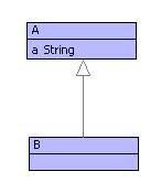
Notice that in both the scenarios given above, it was not necessary for the model element to know about the diagram element and vice versa. This is an important issue: when model instances are synchronized, the machinery must ensure a separation of concerns. There is no reason why the model should know about the diagram – to do so would compromise reusability of the model. Similarly, if the diagram elements are directly associated with the model elements then this makes it difficult to use the diagram model in a variety of circumstances (domain specific languages for example).
2 Models

Figure 2 shows a simple data model consisting of packages, classes, attributes and generalizations. This model is representative of many data modelling notations.
3 Diagrams
Diagrams contain nodes with edges between them. Each node has a position on the diagram and contains a collection of displays. A display has a co-ordinate that is relative to its container; it may be a text item or a box (bordered container of display elements). The model for diagrams is shown in figure 5.


The diagram of the model shown in figure 3 is shown in figure 6. A diagram has a label that is intended to be the same as the name of the corresponding package. Each class is shown as a node and generalizations are shown as edges between class nodes. A class is drawn as a box, with the name as a text item at the top followed by attribute boxes. Each attribute box contains text items for the name, “:” and the type of the attribute. Note that in the example, the positions of the nodes and displays are illustrative.
Diagrams know nothing about classes, attributes and generalizations. This is as it should be since we could choose to use the diagram model to display a variety of information including class-models, snapshot-models, CPM networks and decision trees.
4 Mappings

Figure 7 shows a model of mappings that can be used to synchronize a class-model with a diagram. A mapping is a tree structure that link elements from a left-hand model with elements from a right-hand model. Each mapping has a label that can be used to distinguish between different mappings between the same left and right elements.
Mappings sit between the left and right-hand elements in order to record the fact that they should be the same in some sense. As such, a mapping can have intimate knowledge of the left and right-hand model structures. In the case of a class-model and a diagram, mappings can be expected to know that a class has a name and the related diagram node has a text item that is used to display the class name. Neither the class-model or the diagram model know anything about each other, so there is a clear division of concerns: cross-model information is limited to the mapping.
Mappings can be used to relate any elements from the left and right-hand models and a mapping is is a tree structured thing (made up of maplets). It is up to us as modellers to decide how to structure and use the mapping. Each mapping has children that are other mapping components. The idea is that if the left and right elements are composed of children then the mapping will have maplets that appropriately relate those children. For example, a package may be related to a diagram via a mapping composed of maplets that relate the package’s classes with the diagram’s nodes.
Mappings simply record the associations between left and right-hand elements. There is no requirement for mappings to be used in any particular way. However, it turns out that there are useful patterns of mapping usage, both in terms of how they relate models that are themselves structured using standard patterns.

Figure 8 shows how a package and a diagam are associated using mappings. This is a root mapping and is responsible for synchronizing the package with all its components against the diagram with all its components. The mapping object12 is individually responsible for keeping the name of the package synchronized with the diagram label; it devolves responsibility for the class and generalization synchronization to its child maplets.

Figure 9 shows the child maplets of the root package/diagram mapping. The root mapping has two children:; object14 and object16 that are responsible for associating classes A and B with their corresponding diagram nodes. In each case the maplets have labels (the detail of which is not shown) that identify them as being class-associating mappings.
It is worth considering how this mapping migh be used as part of a tool. Suppose that the name of the package (object8) is modified, to X. The resulting event causes a synchronization to occur (or the user manually causes a synchronization to occur) which in turn asks the mapping (object12) to synchronize its left and right elements. At this stage, the name at object8 is X whereas the label at objct3 is Example. The mapping object12 detects this inconsistency and modifies the label (causing a chage in the GUI). The story would be much the same if the label was changed causing the packag name to be modified.
Now consider what happens if we add a class node to the diagram. Suppose that objects 6, 16 and 10 have yet to be added (i.e. the model contains only class A). The user adds a node to the diagram (object6) and the synchronization is started, as before, at object12.
Part of the synchronization task of object12 is to ensure that, if the diagram has changed, every node has a corresponding class. The mapping object12 can do this because it has access to (and knowledge of) both packages and diagrams. When this check is performed, object12 detects that there is a node (object6) for which there is no child maplet. Therefore, the model and diagram are inconsistent. The remedy is to create a class (object10) and associate it via a new maplet object16 with the diagam node. The story is much the same if a class is added to the model: a new node is added to the diagram and a maplet to the root mapping.
5 Mapping Patterns
Mappings are used to link left-hand instances to rght-hand instances and mappings are structured into trees of maplets. So far, synchronization has been described in rather hand-wavy terms. This is because, in general, many different synchronization strategies and implementations are possible ranging from those that are implemented by hand (and guided by the mappings) to those that are fully automated.
In many circumstances, it is possible to define mapping patterns such that mappings can be applied to instances of left and right models in chunks. Moreover, the pattern chunks can be made to be self manging in terms of synchronization. The next couple of sections show how an analysis of the model-diagram example leads to patterns and then shows how the patterns can be defined in XMF. The following section then gives the full implementation of the model diagram application in terms of the patterns.
6 Equality Pattern
Consider classes and attributes. They have a feature in common: they both have names. Consider class diagrams and the rendering of classes and attributes. They are each rendered as text items in boxes such that the synchronization ties up the name with the string in the text item.
Class and attribute name synchronization is an example of and equality pattern. Where a left-hand item (the name) is defined to be equal to a right-hand item (the string). The difference between the two examples, occurs in terms of how the name/string is accessed, updated and created.
Suppose that an equality synchronization pattern is defined. What are its different modes of operation:
- 1.
If a left-hand instance exists but a right-hand instance does not then the maping is being used to genrate the right from the left. It must be possible to creat a new instance of the appopriate right-hand element and link it to the left with a maplet.
- 2.
If a left-hand instance changes then we must be able to update the right-hand instance.
- 3.
If a right-hand instance exists, but a left-hand instance does not then proceed as for 1 (right to left).
- 4.
If a right-hand instance chages then proceed as for 2 (right to left).
There are clearly two major modes (left, right) each of which has minor modes (in-sync, update, generate). Assuming that it is always possible to tell which side has changed, the two major modes can be defined separately. The following XMF operation definition gives the laft-major mode definition for the equality pattern:
The operation syncEqualLeft takes 5 arguments: a label used to markthe equality maplet; an accessor for the left-hand element; an updater for the right-hand element; a creator for the right-hand element; and a mapping. The mapping associates two elements that have sub-components related by equality. For example, the mapping may associate a package and a diagram such that the name and label are syncronized. For example, the mapping may associate a class and a node such that the class-name and the string in a text item are synchronized.
Line (1) extracts the left and right elements from the mapping. Lines (2-3) select a maplet linking the synchronized elements. If this exists then a check is made at (4) to see if the leftt-hand element has changed. If it has changed then the element will be out of sync with the maplet and lines (5-) update the appropriate components thereby synchronizing.
Line (6) occurs when the maplet for the synchronized elements dos not exist. This occurs when the right-hand element is being generated from the left. In this case, a new right-hand element is constructed (6). Imagine class-names being synchronized with text items: the arguments in (6) are the node and the class-name.
Line (7) creates a new maplet (assumed synchronized) and (8) adds the maplet to the parent mapping.
7 Containment Pattern
Consider packages and classes (similarly classes and attributes) compared with diagrams and nodes (similarly nodes and contained boxes). In both cases one element contains a collection of sub-elements: packages contain classes; diagrams contain nodes. Synchronization of such elements can be captured as a containment pattern with the following modes:
- 1.
Addition of a new left-hand instance (e.g. a class) causes addition of a corresponding right-hand instance (e.g. a node).
- 2.
Deletion of a left-hand instance causes deletion of the corresponding right-hand instance.
- 3.
Addition of a right-hand instance (as for 1 but right to left).
- 4.
Deletion of a right-hand instance (as for 2 but right-to-left).
The pattern can be applied to mny different types of containment structure. The differences occur in terms of access to, creation of and deletion of the contained elements. Also, as for equality, there are two modes depending on whether the left hand element has chaged or the right. The left-hand mode is defined by the following XMF operation:
The operation syncSetsLeft expects 6 arguments:; a label used to tagmaplets; an accessor for components of the left element; a constructor for new right-hand elements; an operation that deletes right-hand elements, a mapping and an element synchronizer.
Line (1) extracts the left and right-hand elements. Each sub-component x is extracted at (2) and handled in turn. A maplet that associates x is extracted at (3-4). If the maplet child exists then the synchronizer is applied to it.
Otherwise (6) creates a new right-hand element, (7) creates a new maplet, (8) adds the maplet to the parent mapping and (9) applies the synchronizer.
Lines (a-f) check whether any children have been deleted from the left-hand element. At (e) a maplet exists for which there is no longer a sub-component x. In this case (e) removes the maplet and (f) deletes the right-hand element.
8 Model-Diagam Implementation
The model-diagram synchronizer can now be implemented in terms of the patterns defined in the previous sections. A synchronizer is an operation that accepts a mapping and synchronizes the left and right-hand elements. The implementation of the synchronizer that is used when a model eleent changes is shown below:
The operation syncPackage causes changes in the package name to update the diagram label, changes in the package classes to update the nodes on the diagram, and chages in the generalization links to cause corresponding changes in the diagram. Each class is synchronized using syncClass.
The operation syncClass causes chages in the class name to update the text in the class node name box, and changes to the class attributes to cause corresponding changes to the boxes on the diagram.
9 A Simple Database Synchronizer
The following shows how the patterns can be used to synchronise packages and classes with database tables. A table is represented simply as a sequence of records. Each record is just a sequence of field values:
Chapter 14 Generating Text from Models
1 Introduction
An important transformation involves turning data into text. The text may be program code, HTML, XML, natural language, or some other format. The output may be an end in itself (for example documentation) or may be an intermediate format ready to be processed by a tool (for example HTML or program code) or may be a save format (for example XML). Many modelling tools provide support for code templates that allow models to be transformed to program code. These are a special case of a model to text transformation.
Often, text is generated by running over the data producing standard chunks of text (or boiler plate) with data inserted at appropriate points. For example, when producing HTML, there will usually be a standard header and standard components of table definitions.
This chapter describes a language construct that allows text to be conveniently produced from models. Furthermore, the construct makes it possible to dip in-and-out of the model and the text interleaved to any depth, making it easy to structure the transformation so that it reflects the text as seen in the output.
2 Examples
Consider the following operation that expects a class as an argument and produces a table definition:
Line (1) introduces a text transformation of type Table. In generala text transformation produces literal text interspersed with text generated by arbitrary bits of XOCL program. Each text transformation differs in terms of the delimiters used to start and end the literal text and the XOCL programs. In the case of Table, the delimiters are ¡, ¿, [ and ].
The arguments used by Table in line (1) are an output channel (to send the text to) and an integer that indicates where the left margin should start. In the example, the left margin starts at position 7: when generating text, whitespace characters up to position 7 are ignored; or, put another way, everything is left-shifted by 7 characters.
Line (2) starts with some literal text (table) that is sent to the output channel. Then the drop delimiters ¡ and ¿ are encountered. The drop delimiters surround XOCL code that produces some text to be sent to the output channel. In this case, the name of the supplied class is generated. Line (2) concludes with more literal text.
Line (3) is a mixture of literal text (a comment) and the path of the supplied class. Line (4) introduces a dropped XOCL expression: a for-loop. Each attribute of the class c produces some text in lines (5-6) which are surrounded by lift delimiters [ and ]. The lift delimiters are used within a dropped expression to surround literal text. It should be noted that lifts and drops can be arbitrarily interleaved.
Lines (5-6) produce text output that describes each of the attributes in turn. Note that the newline at the end of line (5) is part of the output.
Line (7) completes the dropped for-loop. Note that normally an XOCL for-loop is termined by an end keyword. Within a dropped expression, end cannot be used since it will confuse the lifting mechanism (as explained below), so the convention is to use e_nd within lifted text. The only end-keyword that is permitted must be that at the end of the outermost lifted text – line (9).
In review, the Table construct is an example of a model to text template. The body of the template is literal text, up to an open drop delimiter. The text inside the drop delimiter, up to the corresponding closing drop delimiter, is XOCL code (containing e_nd instead of end where necessary). The dropped XOCL code can do anything, but should return a string that is dropped into the surrounding literal text of the template. Within dropped XOCL code, literal text can be used surrounded by lift delimiters. The lift delimiters surround a model to text template (just like Table), however, nested templates can use the delimiters rather than the @TemplateName … end notation. Drops and lifts can be nested to any depth, and in general the actual delimiters used to demote the lift and drop can be defined (so that they do not clash with literal text used in the body of the template). Newlines within lifted text are carried through to the output with the left hand margin affected by the initial value supplied to the template (7 in the example above).
Supplying Class to the Table template produces the following:
Notice how the literal text in the lifted parts has been copied throughverbatim, whereas the name of the class and the names of the attributes have been dropped into the text. The following example shows how drops and lifts can be interleaved to good effect. The aim is to produce an HTML page containing the description of a class. The attributes of the class are to be rendered as a table; each row of the table describes an attribute: the first row is the name of the attribute and the second row is the name of the attribute’s type.

In classToHTML notice how the table rows for each attribute are priduced by a dropped for-loop. The body of the for-loop is a lifted table-row, where the attribute name and type are dropped in. This interleaving is typical of the template mechanism. Notice how the structure of the required output is retained (i.e. an HTML page) where the model data is dropped in at appropriate points. The HTML page for the class Classifier is viewed in a web browser as shown in figure 1.
3 Specification
Code templates can be implemented as a transformation into XOCL code. Each element of the text in a template is turned into a format statement. Literal text ets turned into a format statement that just prints out the text. Dropped expressions are transformed into format statements that evaluate the expressions and then print out their results. The complications arise from keeping track of the indentation and from the interleaving of lifts and drops.
To understand how the transformation works it is useful to look at a few examples. Suppose we have a construct X that is defined to be a template:
is translated to the following code:
produces the following code…
Now, suppose that a simple expression is dropped into the middle…
The output should include the value of the variable named ’dropped’in between the literal text for “Some” and “text.”. Therefore the code that is produced looks like the following:
Within a dropped expression it is possible to introduce a lifted literal:
What we would like to achieve for the nested lifting is the following:
Note that the nested lift, is equivalent to another occurrence of@X … end, therefore we could just produce the following code:
Now we have a general rule for dealing with nested lifts: just wrapthe nested lift up in the appropriate template construct (passing in the current margin for indentation). This will deal with any level of nesting and interleaving:
Is translated to:
which in turn becomes:
4 Design
In order to perform the transformation from a template to code, we must keep track of the level of nesting. This can be done using a simple two-state transition machine. the machine is wither currently lifting or is currently dropping. At each stage the machine consumes input characters until it receives a lifting or dropping token. When it receives a token it changes state. The machine builds literals, lifts and drops. Each time a literal character is encountered it is added to the literal currently being constructed. When the machine encounters an end token, it constructs an appropriate element (either a lift or a drop) and consumes the literal tokens. When the machine encounters a start-token (either lift or drop) then it changes state and starts a new collection of literals:
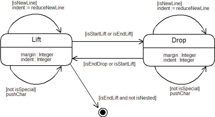
The state machine consumes an input string and produces a code element that represents the structure of the template. The model of code elemnts is shown below:
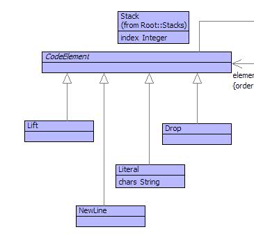
A code element is a literal string containing text that is to be printed on the output channel. Code elements retain newlines so that the indentation can be controlled. The structure of lift and drop blocks in a template is retained by constructing instances of Lift and Drop. An lift or drop object contains a sequence of code elements produced by translating the input string in between the start and end tokens.
For example, the template:
produces the following code elements when processed by the state machine:
Note that the NewLine instances contain two values. The first valueis the amount to left-shift all input. This value is supplied to the template as the argument after the output channel. In the example, @X(out,0) … end supplied 0 as the adjustment to the left-hand margin.
The following example includes further newlines:
and produces the following code elements:
Dropped text becomes wrapped in an instance of Drop:
is translated into the following instance by the state machine:
Finally, if we interleave drops and lifts then these are faithfullyreproduced in the code element structure:
becomes:
5 Implementation
A code template is implemented as a language construct that is defined in terms of tokens for the start and end of lift and drop respectively. The language construct grammar simply consumes all the text in between the start of the template and the keyword ’end’. The text is then loaded onto the machine and the machine is executed to produce a code element. The code element is then transformed into abstract syntax that is the returned by the grammar. Here is an example template:
In the example template X defined above, the start- and end-lift tokensare [ and ] respectively, and the start- and end-drop tokens are { and } respectively. Note how the keyword ’end’ replaces occurrences of the keyword ’e_nd’ before the machine is performed. Including XOCL code in templates must use the keyword ’e_nd’ instead of ’end’ in order that the transation does not get confused.
The mapping is loaded with the token information and the input string. Notice how the input text (protectNewline) is loaded onto the machine by surrounding it with the start- and end-lift tokens. This is because the main body of the template is equivalent to an outermost ’lift’.
The machine is executed with respect to the following state:
The machine constructs values on a stack. At any given time thereis a sequence of code elements being built at the head of the stack. To support this, the machine arranges for the head element of the stack to be another stack onto which the current sequence of code elements are pushed. The following operations manipulate the stack:
The machine needs to recognize when the current position in the inputcorresponds to one of the tokens. a number of token predicates are implemented. All token recognition predicates follow the same basic implementation which is shown as follows:
The machine is implemented using two main operations: processLiftand processDrop. Each operation defines the state-machine processing that occurs when the machine is in the corresponding state. The first operation that is called is processLift (since the complete template corresponds to an outermost lift):
The implementation of processdrop is very similar, however it usesdifferent tokens:
The code elements produced by the machine are translated into XOCLcode. As we have seen in the design, outer-most literals are simply formatted to the output channel. Nested drops are translated to XOCL code that evaluates an expression to produce a string and then formats the string to the output channel. Lifts that are nested within drops are translated to templates are re-processed using the machine. The re-processing is now at the outermost level and therefore produces XOCL code.
The processing is implemented using two code element operations: desugar and dropString. The outermost Lift instance is sent a ’desugar’ message in order to produce the XOCL code:
Desugaring a literal or a new-line is straightforward:
Desugaring an instance of Drop involves inserving the code for thedropped expression and then printing the resulting string to the output channel at run-time. The literals in between the start of the drop and the end of the drop is to be viewed as XOCL code. Therefore we must construct a string containing the code, then turn the string into XOCL code by parsing it. Code elements can be transformed into strings ready for the XOCL parser using the ’dropString’ operation as called in the following operation:
Now we need to implement ’dropString’ for each of the code elementclasses. The result from ’dropString’ must be a string that corresponds to the XOCL code for the element. Literals and Newlines are straightforward:
A Lift is dropped by transforming it into a template construct:
Finally, a Drop generates a drop string by wrapping itself with dropstart- and end-tokens:
Chapter 15 A Problem of Composition
Pattern matching is a useful technique when manipulating data. This chapter describes how to implement pattern directed rules that transform data and how to address a problem that arises with this approach. The implementation also shows how to use operations to delay expressions in rules and how to get the variables bound by the pattern matching into the delayed expressions.
When mapping models to code (and other structured targets) it would be nice of the structure of the target matched the structure of the source. When this happens, individual elements in the source model can be transformed into elements of the target model, and the resulting target elements are then just grouped together to form the result. For example, when translating UML model classes with attributes to Java class definitions, each UML class turns into a Java class definition, each attribute in the UML class produces a corresponding attribute in the Java class. The structure is the same, but the detail of representation is different.
Unfortunately this situation does not often occur. For example, UML models consist of separate elements for classes, associations and state machines; each of these model elements are distinct, but they reference each other. A translation from UML to Java may choose to produce a single class definition consisting of:
- •
Java classes for UML classes;
- •
Java fields for UML class attributes and association role ends;
- •
A state field.
- •
An enumeration in each Java class for each UML message.
- •
A single Java method in a class for handling messages;
- •
A case for each transition within the message handler.
The information in the Java program is nested within the Java class. The corresponding information in the UML model is spread out. The structures are not equivalent.
It is certainly possible to pass tables around the source model and build up the required parts of the target model. However, it is possible to do better than that and to use a language driven approach to hide away the details of how the target model is built up. The transformation language constructs can be pattern directed and the output can be declarative in such a way as to focus on mapping source elements to target elements without having to say too much about the mechanisms by which the output is produced.
This chapter is about the design of a language for producing code for models that solves the composition problem. The structure of this chapter is as follows: section 1 describes a simple executable model and its translation to Java; section 2 describes the architecture of the solution; section 3 describes a language for rule based model transformation and shows how it can be used to implement the transformation rules for the example; section 4 provides the implementation of the language constructs.
1 Translating Executable Models
This section describes a typical scenario where the translation from models to program code requires the target code to pull together information from different parts of the source model. A fully executable program is produced by translating class models and state machines to Java. The example is a car cruise controller and is very simple, but is representative of a large number of strategies for producing programs from models.

Figure 1 shows a simple model consisting of classes, attributes and associations. A car engine controller manages the speed of the car and communicates with the cruise control system. The cruise control system is managed via a mechanical switch on the dashboard.

Figure 2 shows a state machine that defines the behaviour of the engine controller. The engine starts in the Idle state when it is switched on. When the controller detects the accelerator being pressed, it switches to the Accelerate state. When the car is accelerating, the driver can press the cruise control button on the dashboard causing the controller to switch to the Cruise state providing that the speed is less than a preset amount (120). In the cruising state, the driver can switch the control off by pressing the accelerator. When switching to and from the cruising state, the engine controller communicates with the cruise controller, setting its ’on’ state.
Given the behavioural models defined in figures 1 and 2, it is possible to produce a fully executable Java program. The program consists of class definitions for the two classes in the model. Each class includes fields, accessors, updaters and a message handling operation; the definition of these components comes from different aspects of the source model.
The rest of this section shows the program code generated from the Controller class. The example is representative of the code generated from any class in a behavioural model. Firstly, each model class produces a Java class definition (the missing definitions are given subsequently):
The state machine for a class defines a collection of messages onthe transitions. Each of the messages has a unique identifier that is defined as a collection of constants in the class:
The state of an object is given by field definitions that come fromdifferent aspects of the behavioural model:
- •
Each model class defines a collection of attributes with simple types (such as String or Integer); for example the engine controller class defines an attribute ’speed’ of type ’Float’.
- •
The model requires that each object exists in one of a given number of states; for example the engine controller has states for Idle, Cruise and Accelerate.
- •
The model contains a number of associations between classes. The associations allow instances of the classes to communicate with each other. The engine controller class has an association with the cruise controller class with role end names cruise and controller.
The Java field definitions for the engine controller are given below:
Each of the Java fields given above are private to the class definition.To provide access to the state of a Java instance, the following accessors and updaters are defined:
State machines define the behaviour of objects in response to receivingmessages. This can be defined in Java using a method in each class that handles messages:
Each transition consists of source and target states s and t, thetransition occurs when a message m is received and when a guard g is true. When the transition fires, an action a is performed and the receiver changes to the target state t. Each message is implemented as a case in the Java switch statement:
The state machine for the engine controller is shown below:
2 Transformation Architecture
Before looking at a language that supports the generation of code for models, it is worth considering the steps taken by a mechanical process. The idea is that the mechanical process is driven by code generation rules and that the rules encode any domain specific information about the models being transformed. The code generation rules are pattern directed and follow the structure of the source model:
The transformation defined above follows the structure of the sourcemodel. However, the code that is produced (or emitted) by the transformation rules does not follow the same structure; for example fields arising from associations must be added to class definitions that are produced by other parts of the transformation. It is attractive to have the transformation follow the structure of the source model but some technology must be employed to tie up the various target components. An effective way to do this is to use labels: emitted code is labelled and may contain labels, once the labelled target components are produced a subsequent phase is used to resolve label references.

An overview of the architecture of the transformation process shown in figure 3. Model elements are supplied to the rules in the rule base. Each rule consists of a source pattern and a target pattern. Two rules are shown:
- 1.
R1: Pattern P1 matches a class in the model. The output pattern describes a Java class labelled with the class name.
- 2.
R2: Pattern P2 matches an attribute in the model. The output pattern describes a Java field labelled with the name of the owning class.
When model elements are supplied to a rule-base consisting of a collection of rules, each rule is tried in turn. If the input elements match the patterns then the rule is enabled. Patterns contain variable names and an enabled rule has an environment of variable bindings. The first enabled rule is fired. Firing a rule produces a document template by replacing all occurrences of pattern variables in the output pattern. Turning an output pattern into a document template is referred to as forcing the output pattern with respect to the environment.
Figure 3 shows three document templates produced from the rule-base. The first is labelled with classX and is the result of mapping a model class named X to a Java class. The second and third are both labelled with XAtts and are the result of mapping two class attributes named x and y to Java fields. The classX template contains a reference to a label XAtts that is a placeholder for the fields of the class.
A document template is transformed into a document by replacing all label references with documents. This process is called displaying the document template. The display process is shown as the final step in figure 3 where the occurrence of XAtts in the class definition is replaced with all the field definitions labelled XAtts.
Rule firing may involve multiple passes over the data; the output pattern of each rule may refer to other rule-bases (including its own) and supply data to those rule-bases to produce the final document templates. For example, the rule R1 is supplied with a class, emits a document template for the class but also calls the rule-base again with the attributes of the class so that rule R2 fires on each attribute. All rule firing is completed before document display takes place.
3 A Rule Based Language
The transformation from a model to code is performed by a rule-base containing a collection of rules. The rule base is supplied with one or more model elements as input. It tries the rules in turn until one of the rules matches the input. The body of the matching rule is forced to produce a document template. The template may be labelled and may contain labelled placeholders. The rule-base may be performed multiple times against different model elements. Once execution is complete, the templates are displayed by matching placeholder labels against labelled output. The result is an output document with no unresolved labels that can be displayed as text. This section describes the features of the rule-base language and concludes with the complete behavioural modelling rule-base as described in the previous section.
A rule-base with the name N has the following format:
A rule named R has the following format:
where each Pi is an element pattern and each Di is a document pattern.The idea of a rule is that it must be supplied with n inputs. If each of the n inputs match the patterns then the rule is enabled. An enabled rule is fired by forcing the output defined by each Di in turn. The result produced by the rule firing is the last document Dm. Each pattern Pi may contain variables that match against the corresponding input. If the rule is enabled then the collection of variables and values provides an environment for the rule firing.
Here is a simple example of a rule:
The pattern ’x’ matches anything as input. A document ¡ exp ¿ performsthe expression exp in the supplied rule-firing environment. The result of x is either a document or an element that is transformed into a string. In the case of Anything, the rule will produce the stringified version of x as a document.
A pattern may match an object:
The pattern in the rule ToJava matches instances of Class and matchesthe name of the class with the variable ’n’. Two documents are composed using the ’+’ operator. Supplying the class Element to this rule (firing and displaying the result) produces:
Indentation in a document is produced using the matching directives-¿[ and ]:
Supplying Element to the above rule produces:
The nl directive produces a newline and tabs to the current levelof indentation. Collections are processed using the { and } directives:
The { and } contain four components { S M C D } where: S definesthe collection; M defines a mapping that is applied to each element of S in turn; C is a document combinator and D is a default document. The easiest way to understand this construct is via an example. Given a collection S = {x,y,z} then { S M C D} produces C(M(x),C(M(y),M(z))). Given a collection S = {} then the default D is produced.
The collection component S may be a label or an expression. In the example above ¡A¿ is an expression where A is provided by the context of the rule firing. The mapping component M is an expression. The variable map always refers to the containing rule-base and therefore allows the rule base to be applied as part of a rule firing. The combiner nl causes the documents to be combined by joining them together with newlines. The document empty is just that. Note that nl and empty are builtin so we don’t put ¡ and ¿ round them.
Suppose that C is a class with two attributes x and y of type String and Integer respectively. Using the above definition to transform C produces the following (assuming suitable rule definitions for attribute to field transformation):
The ToJava rule above is incomplete since there is no rule for mappingattributes, here they are:
Labels can be used either by themselves in documents or as the sourceof collection templates (as in ¡A¿ above). Documents can be tagged with labels using ’emit’. Here are the class and attribute rules re-written to use labels:
Notice that the mapping components of the collection expression ismodified to become an operation that supplies two elements to the mapping (a,n). Each attribute mapping rule has two inputs: the attribute and the name of the class. The attribute rule emits (and returns) a Java field definition. When a document is emitted against a label (in this case className + “Atts”), it is added to the collection of documents for that label. When the resolution phase is performed, the collection expression will use all of the documents registered against the label.
This concludes the overview of the rule language for transforming model elements. The key features of element patterns are: constants; variables; object patterns with slots. The key features of the document patterns are: literal strings; delayed expressions in ¡ … ¿; combination with +; indentation and newlines with -¿[ … ] and nl; labels with [ … ]; tagged documents using ’emit’; combining collections with { …}.
Finally, the rules for the Java mapping are defined below. There are two rule bases. The first is used to map model types to Java types and the second is used to map packages, classes, attributes and state machines to Java classes. The first rule base is defined in its entirety below and the second is defined on a rule-by-rule basis.
Model types are named elements. The names must be mapped to the appropriate Java types. To simplify the example, sets and sequences are translated to vectors:
A package is a collection of classes, associations and sub-packages.Each package gives rise to a document labelled with the name of the package. The contents of the document are produced by mapping the contents:
A class is transformed into a Java class definition. Some of the componentsof the Java class can be produced directly from the model, other components are produced from model elements that originate elsewhere. The following rule uses labels as placeholders for the program code that is generated elsewhere. The comments in the rule describe each of the major components:
Each attribute defined by a class in the model produces an accessor,an updater and a Java field definition. The methods are labelled so that all accessors and updaters for the class are defined in the same place in the output. The field definition is returned:
An association consists of two ends; each end has a name and is attachedto a type. An association produces a pair of field definitions in the Java classes and also adds accessors and updaters. The transformation is performed by the following two rules:
A state machine belongs to a class and defines states and transitions.The state machine is implemented in Java as an enumerated type for the messages and as a message handling method. Each transition defines what happens when an instance of the class receives a message. A message is defined as an enumerated type implemented as a bunch of constants in the class. A transition is implemented as a case in the message handling method. The rest of the rules define the transformation of a state machine to its implementation.
The following rules produce constant definitions for the messagesused by the state machine:
Finally, each transition produces a case entry in the message handlingmethod of the class. The case checks that the receiver is in the correct state and that the guard is true. If so then the action is performed and the receiver changes to the target state:
4 Implementation
The previous section has defined the syntax of a language for pattern directed document generation rules. The language addresses the code generation composition problem whereby the structure of the input model elements does not match the structure of the output code. Labels are used to tag the generated code (or document templates) and to define placeholders that are then resolved in a subsequent phase.
This section defines the rule-based document generation language. There are several parts to the definition: the language of patterns, the language of documents and the label resolution mechanism. Each of these are explained in turn.
1 Pattern Matching
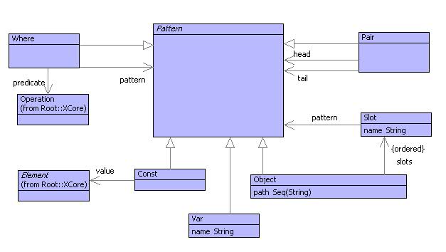
Figure 4 shows the definition of a pattern language. Patterns occur frequently in language definitions where it is useful to extract elements from data depending on the structure of the data. When this is a requirement is it almost always cost effective to define a pattern language and a pattern matching mechanism that it is to write the corresponding program code that extracts the elements each time they are required. For example, the pattern:
is equivalent to the code:
Given that patterns can involve multiple elements and can be nested,the saving in terms of code is quite significant. Furthermore, modelling the pattern language provides other benefits. The language becomes circumscribed and its processing can be very effectively controlled. For example error handling can be reported in terms of the original patterns and not the implementation of the patterns. Optimizations for pattern matching can be universally and retrospectively applied. The patterns can be translated to other implementation platforms, for example by exporting to a programming language.
The simplified grammar for patterns is shown below:
Given an element and a pattern, matching is implemented as a mechanismthat constructs an environment of variable bindings. Each binding associates a variable with a value such that substituting each variable for its value in the pattern produces the original element. For example, given the pattern:
and an instance o of C such that o.x = 10 and o.y = 20 then the environmentassociating y with 20 allows the pattern to be equivalent to the element o. The mechanism is implemented by defining a match operation for each of the pattern classes. Each operation is called match and expects two arguments: the value to be matched and the current variable binding environment. The result of the match is either the variable binding environment or null, if the match fails. For constants:
A variable pattern matches anything:
A pair pattern must match a sequence (and not an empty sequence sincethat is treated as a constant) such that the head and tail of the pattern matches the corresponding elements of the value:
An object pattern matches an instance of the appropriate class whereall the slot patterns match the appropriate slot values:
Each slot matches the appropriate slot value:
2 Documents

Once patterns have matched a collection of elements, document templates are produced in the context of the matched environment. The document model is shown in figure 5. The model is used in three ways: to represent document patterns in rules; to represent document templates; to represent document displays. The difference between these three uses is: patterns may contain delayed expressions; templates may contain unresolved labels; document displays contain no unresolved labels and no delayed expressions.
The classes in the model match the constructs in the language examples from the previous section. The following classes are worth noting: the source, mapper and combiner of a collect are classes that are specialized in specific ways for different kinds of builtin collection operations; Label is a class that is either specialized as a delayed label or a literal label.
Delayed document components are used to allow arbitrary expressions to be embedded. The expressions are to be evaluated when the document is created in the context of the environment produced by successful pattern matching. When the delayed document is created, the expression is turned into an operation whose arguments correspond to the variable names used in the expression. Delayed components include: source, mapper and combiner of a collect; a delayed document; and a delayed label.
The grammar for documents is shown below:
The document grammar extends the OCL grammar in order to refer tothe Exp grammar rule for delayed document components. Many of the grammar clauses for Doc are parameterized with respect to a set of free variables. This feature allows delayed expressions to be transformed into operations where the arguments of the operation are the intersection of the free variables referenced in the expression and those bound in the current pattern environment. For example, the rule:
contains a delayed expression: toUpper(n). The delayed expressioncontains two free variables: toUpper and n. However, when the rule fires, only one of the free variables (n) will be bound in the pattern matching environment. The delayed expression is translated by the parser into an operation:
where the arguments (n) are calculated as the intersection of thefree variables in the body {toUpper,n} and the variables bound by the pattern {n}. Patterns implement an operation FV that calculates the set of variables bound by the pattern; this set is supplied to the Doc clauses. The set FV is ultimately used in the clause DocOp that creates an instance of the class DocOp. A DocOp is just like a normal operation except that its arguments are calculated by taking the intersection of the FV and and free variables of its body.
The rest of the Doc grammar should be self explanatory. Note that some classes are used that are not shown in figure 5. These are sub-classes of Label and collection classes; they capture various special cases and associate them with special purpose syntax.
3 Rules and Rule Bases

Figure 6 shows the model of rules and rule bases. A rule consists of a sequence of patterns and a sequence of documents. A rule base is a sequence of rules that will be tried in turn when the rule base is supplied with elements. A rule base has a table that is used to hold associations between labels and documents when rules are fired. On the resolution pass, labels are replaced with their documents from the table. The table also allows particular documents to be indexed by their name; for example only part of a document in a large model can be re-generated.
The rest of this section describes how rules are fired and then the resulting document is produced by resolving labels. Argument elements are supplied to a rule base via the operation apply defined below.
Each rule is applied to the args in turn until one is enabled by returning a non-null environment. When this occurs the rule is fired, supplying the environment to the rule. Notice that the environment is extended with a binding for ’map’ which allows the document to call the rule-base again:
Rules are matched using the match operation defined below which, inturn, calls the match operation for each of the patterns:
4 Forcing Delayed Documents
A rule is fired by forcing its documents. Forcing a document causes all of the delayed expressions to be evaluated and all ’emit’ documents to update the rule-base table:
Forcing a document achieves two tasks:
- •
Components of a document may be delayed expressions that evaluate to produce documents. These include expressions in ¡ .. ¿ and within the [ … ] part of emit and label references. Forcing a document evaluates the delayed expressions and returns the original document with the delayed expressions replaced with the results.
- •
Components of a document may be ’emit’-ed. Forcing a document updates the document table with associations between the emit-label and the emit-document (after delayed expressions have been evaluated).
Each document class defines a force operation that expects an environment and a table. The environment is produces by the pattern matching and contains values for free variables referenced in the delayed expressions. The table is used to associate labels and documents produced by ’emit’. Many of the force operations just force the sub-components, for example:
Delayed expressions are implemented by associating documents withoperations. The arguments of the operation define the free variables that must be supplied by the pattern matching environment. Components with delayed expressions are implemented in the same way. Here is the implementation of force for a delayed expression that occurs in source code as ¡…¿:
Finally, an emit document updates the table:
5 Displaying Documents
Once rules have been fired and all documents have been forced, the result is a table that associates labels with document templates. A document template may contain label references; it is translated to a document by replacing all the references. This is done using the display operation of the rule base as shown below:
Each of the document classes defined an operation called display thattakes three arguments: the current level of indentation; the table associating labels with document templates and an output buffer. Each of the document classes implements the display operation differently. The rest of this section describes how the documents are displayed.
The Collect class expects the collect source to produce a sequence of documents, each of which is mapped and then combined to produce a final single document that is displayed:
A label reference requires that the label name is a key in the table.The table should associate a collection of documents with the label name; labels are used to reference the first element (collection documents are used to combine multiple document entries in the table):
A NewLine causes a new-line character to be added to the output buffer.After each new-line, the current level of indentation is achieved by adding the appropriate number of spaces:
Ordered documents just display the first and then the second:
Chapter 16 The SECD Machine
There are many different types of model used to analyse programs and programming languages. These include models of source code, e.g. flow-graphs, models of type systems, models of pre and post conditions, petri-nets and various calculi.
Models of programs and their languages are important because designing and implementing programs, as anyone knows who has tried it for real, is a challenging task. The key features of what makes a program work, are hidden away inside a black-box. Even if it was possible to look inside the box, all that would be revealed is a bunch of electronics, memory addresses, registers and binary data.
Programs are not designed in terms of the implementation platform that is eventually used to run the code. A program is defined and implemented in terms of models that describe various abstractions over the implementation platform. The models make programming feasible for humans.
A key model that is used when constructing programs, is the programming language itself. When the code is eventually performed on the machine, the program that was written by the human engineer is certainly not executed directly by the hardware. Over time, languages have been developed that provide abstractions over the implementation platform.
Having said that current programming languages (their libraries and the various software platforms that are currently used) are abstractions; they still must deal with many features of implementation detail that allow the hardware to poke through. Take any serious programming language manual and there will be a section describing how to make the thing run as fast as possible. Use any commercial library (graphics libraries being a case in point) and there will be many features that, whilst they shield the user from the basic underlying hardware, still seem fairly complex.
There is a grand history of models of programming languages. These models are used to understand the fundamentals of what essential features make a program work for an intended application. If you like, these models are an abstraction of an abstraction, but don’t let that put you off; a familiarity with these models is a sure step in the direction of being in-control of a wide range of programming notations.
One of the most important programming language models is the lambda-calculus. It is essentialy a model of procedure-call (and method-call) based languages and has be used to model languages including Pascal, Ada, and Java. There are plenty of texts describing the lambda-calculus and it is certainly not the intent of this book to provide a tutorial. Many of the texts are quite theoretical in nature and should be ignored; pick out some of the more practical looking texts if you are interested, it is certainly worth it.
The rest of this section shows how the lambda-calculus can be modelled. In particular, a machine is developed that runs the calculus. The SECD machine is a fantastic tool to understand how programming languages tick. It is simple and can be extended in a miriad of ways to model useful abstractions of programming language execution.
The syntax of the lambda-calculus is defined as follows:
Where an expression is either a variable (just a name), a function(1 arg and an expression body) or an application (of a function to an arg).
The execution of any calculus expression is also quite simple and takes place with respect to an environment that associates variable names with values. To evaluate a variable, look up the variable name in the environment. To evaluate a function, produce a closure that associates the function with the current environment. To evaluate an application, first evaluate the function and arg expressions to produce a closure and a value. Evaluate the body of the closure-function with respect to the closure-environment extended by associating the closure-arg with the arg-value.
The execution is the essence of programming language execution where procedure (method) calls evaluate by supplying the arguments and then wherever the body of the procedure refers to the argument by name, the supplied value is used instead. Of course there are many caveats and special cases (not least order of evaluation and side-effects), but these can all be dealt with by equipping the basic calculus with the right machinery.

The lambda-calculus syntax is modelled in figure 1. The class Exp extends Syntax so that lambda expressions are self-evaluating. The grammar is as follows:
The definition of Composite provides an interesting feature: leftassociation. Applications are left associative in the lambda-calculus, therefore the expression a b c is grouped as the application a b applied to c, or equivalently (a b) c. The Composite rule is defined using an argument a that accumulates the applications to the left.
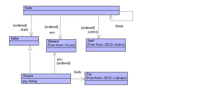
Execution of lambda-calculus expressions can be performed by the SECD machine (whose states are shown in figure 2), so-called because it has 4 components:
- 1.
The stack S that is used to hold intermediate results from expressions.
- 2.
The environment E that is used to associate variable names with values.
- 3.
The control C that is used to hold sequences of machine instructions.
- 4.
The dump D that is used to hold resumptions.

Execution of the machine is performed by case analysis on the instruction at the head of the control. The instructions are shown in figure 3. Any expression is translated into an instruction using Do. the App instruction is used to perform an application as shown below.
The best way to see what how the SECD machine works is to see it running. The following trace shows the execution of an expression (\v. v v)(\x.x). In order to make the output readable, the following pretty-printers have been defined for the various classes: States: (s,e,c,d); sequences: [x1,x2,x3]; pairs: h-¿t; App: @; Do: ignored.
The first thing to appreciate about the evaluation is roughly whatthe expression is doing: the function \v.v v is aplied to the function \x.x causing the function \x.x to be applied to itself producing the result \x.x. Now look at the trace and step through it to see how a machine evaluates the expression. Each step in the trace is a new machine state produced from the previous state by performing a transition. A transition looks at the head of the control in the pre-state to determine the next state.
Line (1) is the initial state. the expression is loaded onto the control. Everything else is empty. Transition (1-2) performs the application expression by unpacking it at the head of the control and adding an @ instruction. Transition (2-3) evaluates the function \x.x to produce the closure at the head of the stack. Notice how the stack is used to hold intermediate results; machine transitions consume 0 or more values at the head of the stack and produce 0 or 1 new values at the head of the stack. Transition (3-4) evaluates the function \v. v v. Transition (4-5) performs the @ instruction by setting up the evaluation of the body of the operator. The state of the machine is saved in the dump so that the return value from the application can be used. Notice how the envirnment in the new state (5) contains a binding for the arg v. Transition (5-6) evaluates the application v v. Transitions (6-9) evaluate the two references to the variable v and then perform the application (again saving the current state for return). Transition (9-10) evaluates the reference to x and (10-11) returns a value since the control is exhausted. Transition (11-12) perfoms the final return leaving the value of the original expression at the head of the stack.
The rules of evaluation for the basic lambda-calculus are very simple. They can be described using pattern matching and are defined in the operation trans below that performs a single transition. A good understanding of the rules of evaluation and their many variations is an excellent basis for a deep understanding of how modelling can inform and enrich programming.
Transition (1) evaluates a variable by looking its name up in thecurrent environment and pushing the value on the stack. Transition (2) unpacks an application at the head of the control. Transition (3) performs an @ instruction at the head of the control. It expects a closure above an argument at the head of the stack. The current state is pushed onto the dump and a new state is created from the closure body and environment. Transition (4) defines evaluation of a function. Finally, transition (5) describes how a value is returned from a completed function application (the body is exhausted).
1 Extending the SECD Machine
As it stands, the calculus and its execution by the SECD machine does not look much like a standard programming language. Using just the features you have seen, it is possible to encode virtually all standard programming language concepts. Doing so is a bit like a cryptic crossword - fiendishly difficult and spectacularly rewarding.
Rather than work with models of programs at the basic calculus level, it is usual to add extensions. In fact, this is where the calculus and its mechanical execution starts to be useful: if you have a requirement to understand or design a new novel feature then see what you need to do to add it to the calculus and SECD machine.
This section shows how the basic model can be extended by adding records, integers and builtin operations such as +. A record is represented as in [age=56, yearsService=10]. A tuple, or vector, is a record where the fields have pre-determined names (usually represented as numbers); for example a pair is [fst=1,snd=2] rather than (1,2). This allows builtin operations to take tuples (represented as records) as arguments: add[fst=1,snd=2] is the same as 1 + 2.

The extensions to the syntax model are shown in figure 4 and the grammar extension is shown below:
The following shows an execution of the expression (\x.\y.add[fst=x,snd=y])10 20. The builtin environment is shown as E. E contains a binding for the name add to the builtin operation for +.
Chapter 17 Modelling with XML Data
There is a general requirement for model data to be interchangeable between tools. This is because organisations rely increasingly on tool chains to support their business. No single tool can support the whole process. Data generated by a modelling tool might hand the information on to a code-generation tool or might hand the information on to an engine that runs the models directly. In any case the different tools in the tool chain need to agree on a format for the data.
In order to have different tools work with shared data there needs to be a common serialization format. Data is serialized when it is exported into a format that can be saved in a file. The format of the data in the file needs to be known to all tools in the chain. The format definition is often referred to as meta-data.
The de-facto standard for data representation is XML. It is a textual format that can be saved to files. Essentially, XML data is a tree where each node in the tree is either raw text or is an element. An element has a tag and some name/value attribute pairs. Each element has a sequence of child nodes. Often you can think of the node tag as the type of the node (for example: an employee record or a customer transaction) and the attribute pairs as containing node properties (for example: the employee name or the date of the transaction). The children of the node usually encode relationships (for example: employee-to-department or transaction-to-product).
XML meta-data (often also encoded as XML) defines the legal structure of the XML documents. For example it defines the set of tags that can be used in elements, the legal set of attributes for an element with a given tag and the order in which child nodes can occur.
Both models and model instance data can be encoded using XML. For example, the UML modelling language has an XML meta-data definition called XMI that defines how UML models are serialized and therefore shared between UML tools.
When using a model-driven approach to system development it is important to understand how to serialize and de-serialize model data. You may be using a standard meta-data definition or be designing one of your own. This chapter describes a number of language driven approaches to using XML data.

Figure 1 shows a simple UML-style modelling language consisting of packages of classes and associations between them. This chapter shows how instances of this language can be serialized as XML data and how the resulting files can be read back into models.
1 Generating XML Data
Given an instance of the modelling language defined in figure 1, the translation to XML data is straightforward. Each class defines an operation toXML that takes an output channel to which XML is written. The format of XML data is standard, so it is useful to define a language construct to support its generation. The following shows how the toXML operation for Package is defined:
The XML construct is used to guide the generation of XML data to anoutput channel. The output channel is supplied in ( and ) after @XML. The body of the @XML construct defines the format of the generated XML data. An XML element has the format:
where TAG is just a name, ATTS is a sequence of attribute value pairs,CHILDREN is a sequence of child nodes and the final ¡/TAG¿ should match up with the corresponding opening tag. In the example, the tag is Package, there is a single attribute called name. The value of the name attribute (on the right of the =) is the name of the package.
The @XML language construct allows XML elements to be written as they will appear in the output, the characters will be send to the supplied output channel. This makes it easy for the system to check that there are no mistakes in the XML format and removes the need for the user to have to use a format-statement or equivalent to describe how the output should appear.
The children part of the @XML construct for packages is an XOCL @For statement that iterates through the package elements and invokes their toXML operations, supplying the same output channel.

Figure 2 shows a simple library model serialized as XML using the toXML operations. Notice that the classes attached to the ends of associations are encoded as the unique identifiers attributes to the classes (in this case the class names are used as the class identifiers, however in a real implementation some unique string is usually used). The rest of this section defines the toXML operations for all other classes in the modelling language.
Associations just wrap an association element around the two ends:
An end generates a name and an identifier for the class that it attachesto. The name of the class is used as the identifier:
A class generates an element with attributes for the name, whetherit is abstract and its identifier. the children are generated by asking each element of the class to generate some XML:
The toXML operations for attributes, operations and arguments arevery similar to those describes above.
2 An XML Generator
The previous section uses a simple language construct to generate XML output. The language construct allows the output from a model to be described in XML format rather than using raw character output. This makes it easier to focus on the structure of the output data rather than the detail of the XML character formatting. This section shows how the construct is implemented.

Figure 3 shows the classes used to implement the XML printing construct. An XML template is a performable expression (out) and a sequence of nodes. The out expression will evaluate to an output channel at run-time and a node is a syntax construct that produces XML output to the channel. A text node is an expression that produces raw text in the XML output. A call node is a general XOCL expression; this allows any code to be embedded in the XML template (such as an @For expression). An element is a syntax construct that formats an XML element to the output channel. The tag and attribute components are all XOCL expressions that produce strings. An element node references sub-elements each of which are XML template nodes.
The XML template construct is parsed by the following grammar:
The grammar extends the OCL grammar that provides the Exp rule; producingan instance of XOCL::Performable. The grammar should be self explanatory; it is worth noting the mechanism by which the template constructs are populated by instances of Performable. The Out rule recognizes an expression in parentheses or returns the expression (via the syntax quotes [— and —]) referencing the standard input stdin. The Tag and AttName rules transforms a recognized name to a string expression.
The grammar synthesizes an instance of the class XML, which is syntactic sugar and transforms itself into basic XOCL code. The Package XML template:
becomes the following XOCL code:
Each of the XML template classes defines an operation named desugar. The XOCL execution engine knows that if it presented with an instance of XOCL::Sugar it will not know directly how to perform the construct. However, the construct will implement the desugar operation that can be used to transform it into something the engine does know how to deal with. The rest of this section describes the desugar operations defined by the various XML template classes.
The XML::desugar operation is as follows:
Each of the XML nodes is desugared and sequenced using the ’;’ operator.The Text::desugar operation is straightforward as it just sends the text to the output:
The Code::desugar operation is also straightforward:
Finally, Element::desugar is where the main work is done. The actionis different depending on whether the sub-elements are empty or not. In the case of no sub-elements:
All the sub-elements are nodes and can be transformed to code viatheir desugar operation:
3 Parsing XML
When XML data is read in it must be recognized against a meta-data description and then the corresponding model data can be synthesized as a result. This is the same activity that occurs when a text language is parsed and corresponding data structures are synthesized. The only significant difference is that instead of parsing a sequence of characters (or tokens) the structure to be parsed in the XML case is a tree of elements. This section describes how the meta-data description for an XML document can be expressed as a grammar including actions that synthesize data. An XML document is recognized and synthesized using a new language construct: an XML grammar; an XML grammar is defined for the simple package modelling language defined in figure 1. This section describes a language construct for expressing XML grammars and shows how it is implemented.
A standard grammar is used by a parser to process an input sequence of characters. A parser follows the rules defined by the grammar, consuming text when the grammar specifies a terminal symbol. The parser takes care to keep track of alternatives; when the parser encounters a choice point, the current position is marked in the input so that the parser can return to the position if the choice fails. The parser encounters actions in the grammar rules, these synthesize elements. The parse succeeds when there is no further grammar elements to be processed; the parser returns the top-most syntheiszed element.
An XML grammar is very similar to a standard grammar with the following differences:
- •
An XML parse processes an XML document which is a tree of elements. The elements that are specified in the grammar and recognized in the parse are elements, element attributes and element children. Unlike text, an element consists of a starting tag (¡TAG¿) and an terminating tag (¡/TAG¿) with child elements in between.
- •
XML documents may include identifier references that are used to encode a graph structure within the tree structure supported by XML. The identifiers are associated with elements synthesized by the parse and must be resolved by the parser.
The following is an XML grammar for the XML document produced in the previous section:
Line (1) introduces the grammar named Models. Line (2) is a typicalexample of a grammar clause; it defines a rule for an attribute. Attributes exist in the XML document as elements with two attributes: name and type. Line (3) declares that an attribute takes the form of an element with tag Attribute and with XML attributes name and type whose values are references as n and t respectively. Line (4) is an action that syntheisizes an attribute; the action may refer to any of the variables that have been bound when the clause matches (in this case n and t).
Attribute is an example of an XML element where the children are of no interest.Such elements are declared in grammar clauses by ¡TAG … /¿. The clause for Class is an example where the children are of interest. Such elements are declared as ¡TAG¿ … ¡/TAG¿. Line (5) declares that the children of a class element must match the elements declared in ClassElement and there may be any number of such elements (as defined by *).
Each class has a unique identifier supplied as the value of the attribute id. Elsewhere in the XML document, classes may be referenced by association ends. The references are made using the identifier of the class. An XML grammar registers a synthesized element against a unique identifier using the declarator :=. Line (6) shows how the class syntheiszed by the Class clause is registered against the value of the variable id. References to the identifier in association ends synthesized by the parser will be automatically resolved as part of the parse. Line (7) shows that a class is synthesized and the elements synthesized by the ClassElement clause are each added to the resulting class.
Line (8) shows the definition ofthe classElement clause. A class may contain attributes and operations. This clause shows how alternatives are declared in clauses using — to sepaate the options. When the parser tries to consume the next XML element against the ClassElement clause, it will try Attribute, if that succeeds in recognizing an element then the parse continues, otherwise the parse will backtrack and try to recognize an Operation.
Line (9) shows the clause for associations. An association end in the XML document references the type attached to the end via its class identifier. An association end element references the class directly, so the identifier must be resolved to the class (which is synthesized elsewhere in the parse). Line (10) shows how the grammar can declare that an identifier reference must be resolved. The class Ref is used to construct an identifier reference. Providing that the identifier in the reference is registered elsewhere in the parse (using := as in line 6) then the parse will automatically replace the reference Ref(id) with the model element registered against the id.
The model for the grammar language is shown in figure XXX.
The grammar for XML grammars is shown below:
A parser for an XML grammar must process an XML document. If the documentconforms to one of the possible trees defined by the grammar then the parse succeeds and the parser returns the value syntheisized by the actions that have been performed. At any stage during the parse, the parser maintains a parse-state containing all the information necessary to continue from this point onwards. The elements of the parse state make up the arguments of a parse operation defined for each class in the XML grammar model. The parse-state contains the following:
- •
The grammar. This is used to resolve calls to clauses.
- •
A variable environment containing the current collection of variable/value bindings. Each time the parse performs a binding of the form v = X, the value of X is calculated (possibly as the result of calling a clause) and the environment is extended with a binding for x. When an action is performed, the variables bound in the environment are made available for reference in the action expression.
- •
An identifier binding containing the current collection of identifier/value bindings. Each time the parse performs an identifier binding of the form i := X, the value of X is calculated and the environment is extended with a binding for identifier i. When the parse is complete, occurrences of Ref(i) are replaced with the value of the identifier i from the identifier environment
- •
A stack of XML input elements. Each time a grammar element of the form ¡TAG¿ is encountered, the stack is popped and the tag of the top element must match TAG. If this fails then the parse backtracks to the last choice point. Otherwise the children of the popped element are pushed back on to the stack and the parse continues with the child elements in the grammar.
- •
A success continuation. This is an operation that represents what to do next in the parse. Each time the parse succeeds, it continues by calling the success continuation. The continuation operation is supplied with parameters: a value; a variable environment; an identifier environment; a stack of XML elements; and, a fail continuation. These arguments represent the parse-state components that are required by the rest of the parse and which may change.
- •
A fail continuation. This is an operation that represents what to do when the current parse fails. A parse fails when the expected tag specified in the grammar does not match the supplied tag in the input element. A parse continuation operation has no arguments; it is simply called when the parse fails.
The parse-state is defined by arguments to the operation parse:
The rest of this section describes the implementation of the parseoperation. The first two definitions are for Empty and Any. Both of these clause patterns succeed; Empty does not consume any input whereas Any consumes the next XML element. Both produce the value null:
An And pattern occurs in a clause when two patterns must occur insequence. The left pattern is performed first followed by the right pattern. If it succeeds, the left pattern may have modified the parse-state; this explains why the success continuation has arguments corresponding to the state that may have changed:
An Or pattern occurs in a clause when there is a choice between twopatterns. The choice involves a left and a right pattern. The parse continues with the left pattern. The right pattern is supplied as the activity performed by a new fail continuation. Notice that the current parse-state is closed-in to the new fail continuation. If the fail continuation is ever called, the parse will continue with the parse-state that is current when the fail continuation is created (not when the continuation is called):
An optional pattern can be implemented by Empty and Or:
When a clause name is called, the grammar is asked for the named clause,a new parse-state is constructed and the clause body is parsed. Variables are local to each clause, therefore when a clause is called the initial variable environment is empty. A new success continuation is created that passes the return value of the clause to the caller, but reinstates the current variable environment:
An action consists of an expression. An expression contains free variablereferences. These come in two categories: those variables bound by the current clause and global variables. An action expression encodes the freely referenced variables as arguments of the operation that implements the expression. Locally bound variables are found in the variable environment. Globally bound variables are found by looking the names up in the currently imported name spaces. The operation Grammar::valueOfVar takes a name, an environment and returns the value (whether it is locally or globally bound):
Variables are bound as follows:
Update works like Bind except that the identifier is bound in a differentenvironment:
An XML element pattern requires that one or more input elements areconsumed. The parse succeeds when the tags of the elements match and when the child element patterns match the child input elements. As part of the match, the attribute values of the input element are bound to the corresponding pattern attributes. The parser is defined below. Notice how the attributes may specify a default value in the pattern; if the corresponding attribute is not available in the input element then the pattern variable is bound to the supplied default value (created by evaluating an expression):
The * designator in clauses declares that the preceding underlyingpattern may occur any number of times. The return value from such a pattern is the sequence of return values from each execution of the underlying pattern. This is implemented as follows. Notice that the failure continuation that is used for each execution of Star(pattern) causes the parse to succeed, but supplies the empty sequence of results. Therefore * cannot fail, 0 executions of the underlying pattern is OK:
Finally, the child of an XML input element may be arbitrary text:
It remains to define how to invoke the parser. A grammar has an operationparse that is supplied with the name of the clause that will start the parse and the name of the file containing the XML document. The class IO::DomInputChannel takes an input channel as an argument and returns an input channel that translates XML source text into an instance of the XML model. The parse operation creates an initial parse-state and then starts the parse by calling the starting clause:
4 Resolving References
A successful parse returns a synthesized value. The value may contain unresolved references to identifiers that were encountered during the parse. An identifier is registered using the i := X construct in a clause and may be used in a synthesized value by constructing an instance Ref(i). Resolving the references involves replacing all occurrences of ref(i) with the corresponding value of X.
Identifier resolution is performed by an operation Grammar::resolve. It is supplied with an identifier environment and a synthesized value. The ResolveRefs walker expects an identifier table (for efficiency), so the environment is translated to a table and then the synthesized value is walked:
Resolving references is easy in a meta-circular environment becauseengines can be defined that process the data as instances of very general data types. ResolveRefs is a walker that traverses the data and replaces all references (or reports an error if unregistered identifiers are encountered). The rest of this section gives an overview of ResolveRefs:
Chapter 18 Interactive Applications
An increasing number of interactive applications can be downloaded onto devices such as mobile phones, PDAs, web-browsers and TV set-top boxes. The applications involve presenting the user with information, options, menus and buttons. The user typically enters information by typing text and choosing amongst alternatives. An event is generated by the user clicking a button or selecting from a menu. Once an event is generated an engine that services the interactive application processes the event, updates its internal state and then produces a new dialog to present to the user.
The dialogs required by the interactive applications tend to be fairly simple and are often used in conjunction with other applications such as being broadcast together with TV video and audio content. The technology used to construct the interactive application should be accessible to as broad a spectrum of users as possible, including users whose primary skill is not in developing interactive software applications.
Technologies used for interactive displays include Java-based technologies such as MHP , HTML, JavaScript etc. These technologies are very platform specific, they include a great deal of technical detail and are certainly not approachable by a non-specialist. Furthermore, the general low-level nature of the technologies does not enforce any standard look-and-feel to interactive applications. The applications developed for a given client (for example a single TV company) should have a common look and feel that is difficult to enforce at such a low-level.
A common way to abstract from technical detail and to enforce a common look-and-feel for a suite of applications it to develop a domain specific language (DSL) whose concepts match the expectations and skill-levels of the intended users. A DSL for interactive applications will include constructs for expressing textual content, buttons, choices etc. The DSL leaves the rendering of the display features and the event generation to a display engine that enforces a given look-and-feel. The display engine can be replaced, changing the look-and-feel without changing the DSL.
In addition to the DSL supporting high-level features for expressing display content, it must provide some means for describing what the application does. Normally, application processing algorithms are expressed at a low-level in program-code. If the DSL is designed with an execution engine then the same approach to abstraction from rendering detail can be applied to abstraction from the operational detail.
An executable DSL is a language for expressing complete applications without detailed knowledge of implementation technologies. The xDSL is a modelling language, instances of which are expressed as data. An execution engine processes the data and runs the application. The xDSL engine can be embedded within devices and other software applications in order to run the models.
This chapter describes the design of an xDSL for interactive applications. The xDSL has a textual syntax and is implemented in XMF. The rest of this paper is structured as follows: section 1 describes an architecture for interactive applications based on an xDSL; section 2 describes the xDSL from the point of view of the application developer, it outlines the language features in terms of a simple application involving a quiz; section 3 describes how the xDSL is implemented on XMF; section 4 shows how the rendering engine can be simulated and connected to the xDSL engine to simulate the execution of an interactive application; section 5 shows how the application models can be serialized as XML; section 6 concludes by reviewing the key features of the approach and the technology used to develop the xDSL engine.
1 Interactive Application Architecture

Figure 1 shows an overview of the architecture for an interactive application xDSL. XMF is used as the DSL implementation engine. XMF provides facilities for developing text-based modelling languages and their associated execution engines. The xDSL is written as a model in XMF, the applications are then loaded onto the xDSL engine and executed.
The application generates display information in a general-purpose format: in this case XML. The XML display information is sent to a rendering engine. The engine understands the display features of the DSL and interprets them in terms of the rendering technology. This achieves a separation of concerns whereby the DSL can focus on the information content and execution logic whereas the rendering engine can focus on a standard way of displaying the information without necessarily having to understand anything about the application that is being rendered.
The rendering engine controls the hardware that interacts with the user. The user generates events that are sent back to the xDSL engine. In principle the events can be very detailed and can be encoded in a suitable DSL. The example presented in this paper uses a very simple encoding of events.
When the xDSL receives an event, it must process the data in an appropriate way to produce more display information for the rendering engine. The processing information is expressed in the application model running on the xDSL engine. The display/event loop continues until the application is terminated.
The architecture shown in figure 1 has been used a number of times based on the XMF processing engine. the development environment XMF-Mosaic is completely based upon a number of rendering engines based on various features of Eclipse: browsers, property editors and diagram editors. The architecture has also been successfully used where XMF is deployed as a web-application and the rendering engine is a standard web-browser (using various combinations of HTML and GWT).
2 A DSL for Interactive Applications
This section presents a simple interactive application expressed using the xDSL and then shows it running. The following section shows how the xDSL is implemented in XMF.
Textual languages are developed in XMF by extending the basic language with new language features. XMF has a small basic language; the rest is developed by extension. Each new language feature starts with a ’@’ character; the feature may be used wherever any normal language construct is expected. In this way, the XMF engine can be developed into any special purpose DSL engine.
The following fragment shows the start of an interactive application (@Model …):
Each model consists of a collection of screens. Each screen describeshow it is to be rendered and how it responds to events. For example, the following screen starts the application. It places some text above a button names Start. When the engine receives a Start event then the application makes a transition to the screen named Question1:
Options are offered using a construct that lists the options (howthey are displayed is up to the rendering engine). The option group is named; the name is used to refer to the particular option value that the user selects when the event returns to the xDSL engine. This is a typical way of encoding variable information during dialogs: http does this and can be used to determine the values of fields and choices on HTML screens. The first part of the Question1 screen uses options as shown below:
Layout can be handled using many sophisticated schemes. A useful,simple way to specify layout is to use horizontal and vertical flow, where these can be nested. The options are displayed below the text in the fragment given above. In the fragment below, the buttons for Next and Quit are displayed next to each other (but below the options):
The Next event is received after the user has chosen an option. Ifthe option is correct then the user is congratulated and the score is incremented, otherwise the user is told the correct answer. In both cases the dialog continues with the next question.
Actions may be conditional, the conditional expression may refer to choice variables, values of variables passed to screens and the current state of the model instance. Actions may also produce displays (without having to go to a new screen) this allows variables to be scoped locally within an action 11 1 We really should have a let-construct and some local variables here to show that the nested display has access to locally-scoped variables over a user-transaction.. In the following, the Next action has two local displays that are used to respond to the choice:
That completes the overview of the DSL for interactions. It is simpleand closely matches the concepts required to define an interactive application. It includes execution by encoding event handlers. It deals with complexity by being simple and supporting nesting with local scope and modularity. A non-expert in interactive software applications should have no problems writing an application in this DSL.
The following shows run-fragment of this application. Since there is no rendering engine attached, the XML is printed and the responses encoded by hand:
3 Implementation
The implementation of the xDSL has two main components: a syntax model and a grammar that transforms text to instances of the syntax model; and, a semantics model that defines an execution engine. The syntax model defines a modeling language that defines an application type; an instance of the type is defined by the semantics model. This is a typical way to define a language: models represent things that can be performed in some sense. Performing the models produces instances whose behaviour is expressed by the model. Another way to think about this is that we aim to produce libraries of reusable interactive applications (instances of the syntax model). A run-time occurrence of an application is described by the semantic model.
XMF provides facilities for working with text including grammars, XML parsers, XML formatters etc. The models have been developed using the XMF development engine XMF-Mosaic and then run on the basic engine.
1 Syntax
The syntax for the DSL has two parts: the abstract syntax and the concrete syntax. The abstract syntax consists of a collection of models that are described below. The concrete syntax is defined by a collection of grammars that are defined at the end of this section.


Figure 2 shows the top-level model for the interactive application language. A model consists of a collection of properties and a collection of screens. Each property is defined by the model in figure 3; it has a name and a classifier. XMF has a meta-model that provides features such as Class, Object etc. A type is called a Classifier in XMF; Integer, String, Set(Object) are all XMF classifiers.


Screens are shown in figure 4. A screen has a collection of arguments. An action may cause the application to make a transition to a screen in which case the transition can supply argument values to be used when calculating the display for the screen. Figure 5 shows the model for displays. Each element of the displays model can produce some XML output that is understood by the rendering engine. In addition, some of the display elements are associated with actions that will be performed when the appropriate event is received by the xDSL engine.
The display elements of an application model refer to an XOCL class called Exp. This is used wherever an executable fragment of code is required. It allows features of the displays to be computed dynamically. For example when a transition to a screen is made, the names of the buttons may depend on the values of the arguments that are passed to the screen. This is the reason why a button has an exp: it is used to calculate the label on the button in terms of the variables that are in scope at the time22 2 Unfortunately no examples of this feature are given in the document. However, imagine a list of voting options that will depend on the current state of the system.. The Exp class is a way of importing the models for XMF expressions into the displays model.


Menus are shown in figure 6, each menu has a label that is computed (again depending on the context) and an action. Actions are defined in figure 7. An action is either a transition to a new screen (Go), a conditional action (If), an update to a variable currently in scope (Update) or a local display.
The developer of an interactive application does not directly create instances of the abstract syntax model. The idea is that they write in a text language that is parsed to synthesize instances of the syntax model33 3 Another way of doing this is to use some form of graphical notation. XMF is designed to interface to EMF and GMF and therefore provide execution engines for models defined in EMF. The interaction language seems to lend itself more to a textual representation due to the actions and nesting that needs to be expressed..
XMF allows any class to be extended with a grammar. The class then defines a new syntax construct that is completely integrated into the base language of XMF. Any number of classes can be added in this way and new syntax classes can build on existing syntax classes. The following is a simple example of a class definition that implements a simple guarded expression:
where e1 evaluates to produce an object to which we want to send themessage m with args e2,e3 and e4. However, e1 might produce null in which case we don’t want to send the message, we want to do e5 instead. This language construct is implemented as follows in XMF:
The key features of the NotNull class are as follows:
- •
The class extends Sugar which means that it is defining a new syntax construct by providing an operation called ’desugar’ whose responsibility is to turn an instance of NotNull into program code.
- •
The grammar definition extends the OCL grammar and thereby imports all of the basic grammar-rule definitions. This provides the rule for Exp which is the top-level grammar-rule for all language constructs.
- •
Each grammar-rule consists of a name and a body. The rule may optionally have arguments. The body consists of terminals (in ’ and’), builtins such as Name, rule-calls (possibly with arguments) and actions (inside { and }). The rule actions are any program expression, in most cases they use class-constructors to create an instance of a named class.
- •
The desugar operation uses lifting-quotes ([— and —]) to create an instance of syntax-classes. The opposite of lifting is dropping (¡ and ¿) used to calculate syntax by evaluating an program expression.
The rest of this section describes how the grammar feature of XMF can be used to define the interaction language. A model consists of a name followed by properties and screen definitions:
A property is a name and a simple expression (that cannot includethe ’;’ operator). The property-rule action uses an interesting feature of syntax classes that allows the expression to be dropped into the syntax element and is thereby evaluated to produce a classifier for the property type:
A screen has a name, arguments, menus and display elements. The rulefor screen arguments shows how optional elements are processed: it returns either a non-empty sequence of names Seq{a—as} (head followed by tail) or the empty sequence Seq{}:
A menu is shown below. This shows how expressions are captured indata. The rule for a menu item name returns an instance of the class Exp that is used in data to wrap an evaluable expression. There are two forms of construction for Exp: Exp(e) and Exp(e,V,null). In both cases e is an instance of a syntax class. In the second case V is a collection of variable names that occur freely in e. The values of variables in V can be supplied when the expression is evaluated (via keyApply as shown below).
Another interesting feature of the menu item name rule is the use of ’lift’ to transform a data element (in this case a string n) into an expression whose evaluation produces the original data element:
Since Display is an abstract class, the grammar-rule for Display isa list of concrete alternatives:
Action is another example of an abstract class:
2 Semantics

The semantics of the interactive application modelling language defines an instance model for the syntax and also defines an execution engine for the instances. The instance model is shown in figure 8. An instance of a Model is defined by the class Instance, it should have a slot for each property of the model. The value of each slot should have a type that is defined by the classifier of the corresponding property.
The class Engine defines the execution engine. An engine controls an instance and maintains an id-table that maps event ids to handlers as shown below. The idea is that each time an event occurs, a handler from the id-table is used to produce a new XML display that is sent to the rendering engine. The XML data is calculated from the information in the model and the current state of the instance slots.
The rest of this section defines the engine execution semantics; the following section shows how the engine is connected to a rendering engine. The engine processes a screen-transition using the ’go’ operation defined below. XMF supports many types of input and output channel; this operation shows an example of a string output channel used to capture and then return the XML output data as a string:
An instance handles a screen-transition by looking up the screen inits model. If the screen exists then it is requested to display itself with the supplied argument values:
A screen delegates the ’display’ message to its underlying displaycomponent. The screen argument names are bound to the argument values to produce an environment of bindings using the ’env’ operation:
Each display element type : Button; Text; Horizontal; Vertical; and,Options implements a ’display’ operation that writes XML data to the supplied output channel. As a side effect, if any of the elements have event handling actions then the engine is updated with an appropriate handler for the event when it is received from the rendering engine.
Each ’display’ operation shows the use of an XMF language feature @XML … end that is used to write XML output to a channel. The construct has the form:
where the literal XML data is written to the supplied output channel.In-between writing the starting tag and ending tag, an arbitrary program is processed.
The ’display’ operation for text shows an example of the shortenedform of @XML … end and also the use of the ’keyApply’ operation of the Exp class. The ’env’ argument supplied to ’display’ contains bindings for all variables in scope. The ’keyApply’ operation performs the expression in the context of these variables:
A button contains an action that is used to handle the event arisingfrom the user pressing the button in the rendering engine. The ’display’ operation for Button shows how an event handler is registered in the engine. The arguments passed to ’registerActions’ are the context required to perform the actions when the event associated with ’id’ is received:
Horizontal and Vertical are similar:
the ’display’ operation for Options shows an example of interleavingof XML and program code:
The ’registerActions’ operation of Engine must define a handler foran event. The definition associates the event identifier ’id’ with an operation in the id-table of the engine. Actions are performed using their ’perform’ operation which expects to receive arguments that include the current environment of variable bindings. The variables available to an action include all those bound by selecting options on the display. These display-bound variables are supplied to the handler (in the same way that http works) as an environment ’env2’:
There are four types of action: If; Update; Go; and, Display. Eachaction produces a result and the last action performed should return an XML string to be sent to the rendering engine. If performs one of two actions (or nothing) depending on the outcome of a test:
An update changes the value of a variable currently in scope. Thevariables in scope are: the slots of the instance; the current screen arguments. The following operation checks whether the named variable is a slot and updates the instance appropriately, or updates the current environment:;
Go makes a transition to a new screen. The screen will produce theXML output. Notice that the current ’env’ is not supplied to the ’go’ operation; therefore any variables currently in scope are not available to the target screen unless their values are passed as arguments:
Display is a way of locally displaying a screen without losing thevariables that are currently in scope:
3 Handling Events
Events occur when the user interacts with the rendering engine, for example by pressing a button. When the event occurs, the current screen may contain any number option groups. Each option group is named and offers a number of alternative values. The selected option may affect the behaviour of the engine in terms of variable updates and screen transitions. Therefore, the event sent from the rendering engine to the xDSL engine must encode the value of any option variables currently displayed.
In addition there may be any number of ways an event can be raised: menu selection or button press. Each must be uniquely identified and the event must supply the identifier of the event that occurred.
An event is defined to have a format that starts with the event id and is followed by any number of option variable/value pairs:
The event is encoded as a string and must be decoded by the engine.This is easily done by defining an event as a grammar-rule:
When an event is received by the engine it is supplied to ’getDisplay’which calculates a new XML display string for the rendering engine. The operation uses the grammar defined above to synthesize a pair Seq{id—env} containing the event id and an environment of option-group variable bindings. If the id is bound in the id-table then the handler is supplied with the environment:
4 Simulation
Figure 1 shows the architecture of an interactive application. The rendering engine is external to the design of an xDSL; the relationship between the two is defined by the XML schema for the display language and the format of event strings. However, it is useful to be able to simulate the rendering engine in order to test the xDSL engine. This can be done by setting up a simple test harness for a pair of data consumers and linking the xDSL engine with a rendering engine simulation that reads events strings in from the terminal.
The following class implements a data producer-consumer pair:
The filter operation is used to generate data that is supplied tothe other consumer. If a pair of Consumer instances are linked together then the data will bounce back and forth as required. The following operation creates a filter for the xDSL engine:
The following filter operation simulates the rendering engine. Itdoes so by pretty-printing the XML to the standard-output. An XML string can be transformed into an XML tree using the ’asXML’ operation defined for String. The standard-input is flushed and a line containing the event is read and returned:
Given a model ’model’, the following code produces, and starts, asimulation:
5 XML Representation for Applications
A requirement for interactive applications is to be able to dynamically update the content and to be able to transfer the content from remote locations in a standard format. The application describes in this paper is completely represented in data. This means that, although the application is executable, it can easily be serialized, send over a communications link, and then uploaded onto the device that is running the xDSL engine.
XMF provides support for encoding any data elements as XML. There is a basic markup provided for all XMF data; the mechanisms for which can easily be extended to provide bespoke XML encoding. Using the basic mechanisms, a model can be encoded as follows:

The resulting output is produced in an XML file that is shown in figure 9. The XML markup shown in the figure is the default vanilla-flavour markup provided by XMF. It is possible to add adapters to an XML output channel that filter the data as it is processed and thereby use domain specific markup. So instead of seeing Object and Slot as element tags, we might use Screen and Button.
The XML can be read back in using the following code:
6 Conclusion
This chapter has described an approach to modelling systems whereby an engine for an executable domain specific language (xDSL) is used to develop and run the applications. The xDSL is designed to use concepts that are suited to the application domain which allows the language to abstract away from implementation details; the language is then executable, can be used with different implementation platform technologies, and is suitable for use by people whose primary skill lies in the application domain rather than the implementation technology.
A method for developing xDSLs has been shown that involves a separation of concerns between syntax elements that describe type-level features of a model, and semantics elements that define run-time features of an application. Experience has shown that this separation is natural and allows the xDSL developer to effectively manage the process.
We have shown how a textual syntax can be added to an xDSL. In practice, most xDSLs will require a concrete syntax. The precise form of this will depend on the nature of the application and who the intended users are. Sometimes, a purely graphical syntax is appropriate (for example UML class-diagrams). Other times a purely textual syntax works best, especially where executable features are involved and when complexity can be controlled effectively using textual nesting. Often there is scope for a mixture of the two where different aspects of the models are constructed using graphical or textual syntax.
Modelling all features of a language has a number of benefits that arise because everything is reified. Reification involves representing everything as data as opposed to program code or transient non-tangible artifacts such as system events. Once everything is reified, many types of analysis are possible including well-formedness checking, type checking, application of style rules. It becomes easy to capture and apply patterns and to perform refactoring. All features of an application can be transformed to a target technology.
Modelling actions is particularly important here; often actions are left as unprocessed strings of program code which makes it very difficult to analyze and run as part of an xDSL engine. The application given in this paper has shown that it is straightforward to model actions and to integrate them into the execution engine for an xDSL. By following a few basic guidelines in terms of variable scope and control flow, actions are easy to implement and are completely integrated into the xDSL, its analysis and transformation.
Chapter 19 Choosing Between Alternatives
Processing information is a linear activity. Listen to anyone describing how something is performed and you will hear phrases like: ’first get an X, turn it into a Y and feed it into the Z’. This is great because mechanical processing of models is a linear activity too; there is a close correspondence between real-world processes and their modelled equivalent.
However, things are often not that simple. On closer inspection a process can often be more like: ’select an X, find a way to turn it into a Y and feed it into one of the Zs’. In this case processing is not so obviously linear. What happens if the X that is selected turns out to be the wrong choice when trying to make a Y? Can we go back and try another X? If no Z is available who is at fault: the X or the choice of Y?
The world is full of choices. Modelling the world often needs to take account of choice. Once choice is admitted into a process, the scope of the choice becomes an important issue. How far can processing proceed before a particular choice cannot be undone? In a linear activity, undoing a choice within a particular scope is called backtracking, i.e. returning to the last choice point, selecting an alternative and re-processing from that point.
Choice (or equivalently non-determinism) is a property of a model. Backtracking is a property of the execution engine for the model. Backtracking is a way of implementing choice as a linear activity; it is an important and often occurring pattern. This section is about how to implement the pattern.
1 A Choice Pattern
Choice tends to occur as a pattern involving:
- •
A collection of elements to choose from (or alternative actions).
- •
Something to do next with the selected element.
- •
Something to backtrack with (a failure).
Each use of this pattern tends to be slightly different in the detail. But the principle is generally the same. The pattern can be encoded as follows:
The operation select (1) encodes the pattern. It takes 3 arguments:S a set of elements to choose from, the activity to do next and a fail for backtracking. The next activity is encoded as an operation that is expecting an element and a fail. The fail argument is encoded as an operation that takes no arguments and jumps to the last choice point to choose an alternative.
The idea is that the next operation contains all future processing for a selected element. Cruicially, the next operation may be invoked more than once with different choices from S. Lines (4-6) show this occurring, where an element e is selected from S and supplied to next. The failure argument supplied to next is a new choice point; if it is ever invoked then select is called again with fewer options to choose from, but the same next and fail. Therefore, select can cause the same next argument to be invoked multiple times with different elements chosen from S.
If select is ever invoked with no options (2) then the initial failure argument is chosen. This allows chaining of different uses of select.
A slight variation on this pattern is the inclusion of a predicate that controls whether the chosen element is valid or not:
The predicate is used in (6) to test the element. If pred is satisfiedthen next is invoked as before (7), otherwise alternatives are tried (8).
This pattern can be encoded as a language construct. The basic mechanism involves repeated selection from a supplied set of alternatives. The grammar below uses a locally defined recursive operation to continually backtrack though the elements of a supplied set:
Instead of defining a selection operation each time choice is used,the selection construct can be used as follows:
The variable e is initially bound to an element selected from theset S and the body of the construct (after the do) is performed. The variable f is bound to an operation; is f is ever invoked (with 0 args) then another element of S is selected and the body is performed again. Subsequent uses of f have the same effect until S is exhausted at which point the alternative part of the construct (after the else) is performed.

Consider a situation, shown in figure 1 where two sacks contain an arbitrary collection of numbered balls. Balls are selected from each sack in turn and placed in a line. The idea is to wind up with a sequence of balls whose numbers form an ascending sequence.
Since it is not permitted to look inside the sacks when selecting a ball, things can go wrong at some point during the process; although it is always possible to select the balls in a way that achieves the desired outcome. If things go wrong then balls can be put back (balls are appropriately marked as to which sack they came from), and the selection restarted from any point.
The sacks can be modelled as follows:
where two sacks are set up as follows:
The process of selection is to be modelled as an operation on Sackthat builds a sequence of integers (balls) by ping-ponging between the receiver and ’other’, each optionally adding an integer. What happens when there are balls left to choose, but which cannot be added to the sequence because their numbers are too low? Is it always possible to select so that this situation does not occur? Inspection of the rules shows that this is not the case (the contents of the other sack cannot be inspected). Therefore, a stalemate situation can occur, therefore backtracking is a candidate modelling technique.
The rest of this section builds up the implementation of an operation defined by Sack for ordering the elements selected from two sacks. The operation is called with no arguments:
The ordering operation needs to initialise the ordered balls and createan initial next and fail. Line (1) calls a second Sack operation called order that has these as arguments. The initial collection of ordered balls is Seq{} (1), the initial next operation and fail are supplied in lines (2) and (7).
In this example, each next takes 3 arguments: the current sequence of ordered balls, a next for the other sack and a fail. At line (2) the initial next calls the ordering operation for the other sack (3) passing it a next at (4) that ping-pongs back.
The initial fail (7) returns an error value because it should always be possible to order the balls, i.e. this should never occur.
The second order operation is defined as follows:
If the other sack is empty (1) then the selection continues with thecurrent sack (7). If the other sack is not empty then there is a choice: add an element from the current sack (2) and continue or just continue. This alternative is encoded by extending the fail (3) so that if things go wrong, the curren sack is skipped. If it is skipped then play resumes with the current sack due to the next continuation (4-5).
The final operation uses Select to continually select from the available balls:
2 Finding a Route

Figure 2 shows a map of the UK with locations and roads. One way of modelling this information is using the graph construct defined in section :
Each node of the graph is a city. Each edge of the graph is a roadlabelled with its name. For example from London it is possible to go to Brighton using the M23 (and vice versa), and possible to go to Bristol using the M4.
Consider how to find a route from one city to another. Suppose you want to get from London to Carlisle. It is possible via the M1, A1 and then A69. Alternatively, you could go A1, A1, A69. In principle there are many routes between two cities. Ignoring distance and other criteria that might lead to selecting one route over another, the only rule that should be applied is that a route does not pass through the same city twice.
How might the construction of a route be modelled? Given a start and end city, if there is a road linking the two then a route is found. Otherwise, any road from the start (or end) can be selected leading to a new start (or end) point. Given the new start (or end) then the process can be repeated until it can be shown that no route exists (remember you cannot go through the same city twice) or a route is found. Given that choices are made, if no route can be found then backtracking can b employed to return and make an alternative choice.
The class Routes extends Graph with an operation for finding a route:
Given the names of the source and target cities (1), a route is consructedby calling another operation with a set of used roads, the source, target, a next (3) and a fail (5). The initial fail is invoked when no route exists, it returns the special no-route-available value NONE.
A next expects a set of used roads, a path and a fail. The path links the source and target cities and is a sequence of road names.
The second route operation is defined below:
3 Explanation and NoGood Sets
Patterns of search (as described above) can be encoded using language constructs. Typically these involve success and failure continuations that maintain the state of the search and provide a convenient mechanism for branching. Continuations make it easy to backtrack when it is found that an incorrect branch has been selected. These techniques work well for finding a configuration amongst a number of alternatives such that the configuration satisfies a given condition. However, extra work is required to explain the lack of a satisfactory configuration.
One technique is to invert the condition that selects a correct configuration and to use it to explain why no satisfactory configuration could be found. Instead of selecting a single satisfactory configuration, such an inversion produces a collection of configurations, each of which has a problem. Such configurations are sometimes referred to as noGood sets. This section describes an application that uses search to select a configuration of business components; noGood sets are used to explain why a solution cannot be found.
Consider developing a business plan. The business must set out its goals in terms of what the business wants to achieve. Each goal is supported by a collection of tactics each of which describes an activity or approach that claims to achieve the goal. In addition, a goal may be decomposed into a collection of child goals; achieving all the child goals individually is the same as achieving the overall goal. In order to implement a given tactic it is necessary to allocate some resource. Resource is provided by organizational units, which may be company departments or individuals.
A goal may be achieved if it has a supporting tactic that is adequately resourced; or may be achieved if all of its children are achieved by the same rule. It is important that a company does not over-commit its resources, therefore a goal can only be achieved if the unit resource limits are not exceeded.
Here is a high-level goal for a telephone banking business:
![[Uncaptioned image]](1506.03363v1/LanguageEngineering/Choice/Images/Goal.jpg)
The business will be successful if it has happy customers. This goal can be decomposed into any number of sub-goals:
![[Uncaptioned image]](1506.03363v1/LanguageEngineering/Choice/Images/SubGoals.jpg)
where a customer is happy if their calls are answered effectively and their complaints are handled. Each of the sub-goals has any number of tactics that will achieve the goal:
![[Uncaptioned image]](1506.03363v1/LanguageEngineering/Choice/Images/Tactics.jpg)
Finally, the tactics need to be resourced by an organization unit. A unit may resource more than one tactic and a tactic may be resourced by more than one unit. In this case the unit is a telephone call centre:
![[Uncaptioned image]](1506.03363v1/LanguageEngineering/Choice/Images/Units.jpg)
The models shown above can be used as part of a business as a decision support solution. Each model describes the goals the business intends to achieve and how the goals are to be implemented and resourced. The solution provides feedback in terms of the options for resourcing the tactics that achieve the goals. If the goals cannot be achieved then the solution will provide feedback on why the different resourcing options fail.
The rest of this section is in two parts: the first part describes how an engine is defined that finds a resourcing solution; the second part describes how noGood sets are used to provide feedback when there is no solution.


Figure 3 shows a model of the business concepts used by the solution. Figure 4 shows a report model that is produced when there is a solution consisting of a collection of results each of which associates a goal, a tactic and an organization unit.
The following rules are applied to find a solution. A goal g is achievable when:
- 1.
g is supported by at least one tactic that is established by at least one organization unit; or
- 2.
g has at least one sub-goal and each sub-goal is achieved; and
- 3.
the number of tactics supported by each unit does not exceed the resource for the unit.
The rules are implemented as an operation called achievable that is defined below. The arguments of the operation form the context for the achievable-engine. It is supplied with a goal, a table of resources, the current results and continuations for success and failure. The table of resources is an a-list mapping unit names to the current amount of resource available for that unit. The results are just a collection of result instances.
The success and fail continuations are used to implement a backtrackingmechanism. The rules are implemented by the achievable-engine in terms of search. A choice-point arises when there is more than one tactic that could be chosen to support a goal and when there is more than one unit that could be chosen to establish a tactic. In both cases, one of the options is chosen and a choice point is created that will be used if ever the search fails.
Failure occurs when a goal cannot be achieved because it has no tactics or a tactic has no establishing unit. The resource associated with a unit is reduced by 1 each time the unit is used to establish a tactic. Once the count reaches 0 the unit cannot be used again; a subsequent attempt to select the unit causes backtracking.
The achievable-engine uses language constructs that are specifically designed to support the business solution. These constructs are: Select which is used to select from a collection; Result which is used to produce a result; Use which is used to reduce the amount of available resource for a unit; Unless which is used to place a guard on an action; and, ForAll which is used to require a condition holds for all element of a collection. These language constructs use the arguments of the engine as ’globals’ and are implemented as follows.
The language construct for Select uses the selection operation to try each element of a collection:
The desugar operation for Select builds up a choice-point throughthe fail continuations:
The Result construct adds a new result to the current collection ofresults. This establishes a new collection of results for the scope of the Result body:
When a unit is used to establish a tactic, the number of resourcesassociated with the unit must be reduced by one. However a unit cannot use more resource than it owns, therefore if the resources are exhausted for the required unit then engine uses fail to select an alternative:
The Unless construct simply places a guard on an action; if the guardfails then an alternative is found using the fail continuation:
The ForAll construct requires a condition to hold for all elementsof a collection. This is achieved using the success continuation; each element of the collection is selected and the success continuation returns to the collection to try the next element:
That concludes the language constructs for the achievable-engine.The search is controlled using continuations so that all possible combinations of goal, tactic and unit are tried to see if they are compatible. When an illegal combination is encountered, the fail continuation is used to backtrack. Therefore, the engine will find a suitable collection of results if they exist.
When no suitable combination of business elements exists, the engine returns no value. It simply reports that the goal cannot be achieved. The rest of this section describes how a noGood sets can be constructed to explain the reasons why a solution cannot be found.
A noGood set is a combination of goals, tactics and units that invalidates the achievable rules defined earlier. The rules are invalidated when a goal has no tactics, when all tactics for a goal lack suitable organization units, or when all the sub-goals of a goal invalidate the rules. When no valid solution can be found for a goal, it is safe to assume that at least one noGood set exists for the goal; there may bemore than one noGood set and it is useful to report all of them.
The following operation constructs the noGood sets for a goal:
There are four reasons for a noGood set. Each reason is implementedas a separate operation. The first operation constructs a singleton set Unachievable(g) when the goal g has no tactics and no children:
If a goal has a tactic with no establishing units then a noGood setcontains Unestablished(g,t):
If a goal has a tactic with a unit then, since we know that thereare no good sets, the unit must be overused (or the noGood set is incomplete). The following operation records allocations that will become illegal when combined with other elements:
Finally, each of the children of a goal must fail in a noGood set.The following operation calculates the noGood sets for each child and then combines them:
Finaly, each noGood set must be interpreted to produce an explanationof why a good set could not be produced. The following operation translates the noGood sets into strings that explain why each fails:
Chapter 20 A Command Language
When modelling applications there is often a requirement for some kind of command language. UML, for example, has state machines where the actions on the transitions are written in an action language and describe what happens to the state of the system when the transitions are fired. One way of providing support for actions in a model is to allow the user to write commands in their favourite programming language; the commands are represented in the model as strings. This is a very weak form of command language, since the strings cannot be processed easily by the modelling engines. Typically they cannot be performed at all until the models are exported as program code, where the command strings are simply embedded in the output.
More flexibility is provided by modelling the command language. The model instances can then be interpreted by an engine as part of performing the overall model. Furthermore, since the commands are modelled, they can be analysed in various ways and transformed to different target implementation languages rather than being limited to one.
This chapter is concerned with writing interpreters (translators and compilers) for a command language. When defining an interpretive semantics for a language there is often a similar language at hand (at least the language in which the interpreter is written).There is a choice choice as to whether the syntax structures are directly interpreted or whether they are translated to syntax phrases in the existing language. The advantage of a translational approach is that the execution engine for the target language already exists and is probably more efficient than any interpreter we could write for the source language.
Compilers are translators for languages where the target language is usually highly optimized and very different from the source language. In principle, however, there is no essential difference between a translator and a compiler. A language that uses the translational approach to target a sub-language of itself is often referred to as desugaring the source language.
1 XCom - A Simple Command Language
XCom is a simple command language with values that are either records or are atomic. An atomic data value is a string, integer or boolean. A record is a collection of named values. XCom is block-structured where blocks contain type definitions and value definitions. XCom has simple control structures: conditional statements and loops. The following is a simple example XCom program that builds a list of even numbers from 2 to 100:
XCom expressions evaluate to produce XCom values. Values are definedin the Values package and which is the semantic domain for XCom. Values are either atomic: integers and booleans, or are records. We use a simple representation for records: a sequence of values indexed by names. XCom records are created by instantiating XCom record types. A record type is a sequence of names. Types raise an interesting design issue: should the types be included as part of the semantic domain since evaluation of certain XCom program phrases give rise to types that are used later in the execution to produce records. The answer to the question involves the phase distinction that occurs between static analysis (or execution) and dynamic execution. Types are often viewed as occurring only during static analysis; although this is not always the case.
We will show how the semantics of XCom can be defined with and without dynamic types. All XCom values are instances of sub-classes of the class Value.
Record types are sequences of names. Records are sequences of valuesindexed by names; the names are found by navigating to the
type of the record:
A new record is produced by performing a newexpression. The type to instantiate is given as a string. An alternative representation for types in new expressions would be to permit an arbitrary expression that evaluates to produce a type. This design choice would rule out static typing and force the language to have dynamic types. We wish to use XCom to illustrate the difference between dynamic and static types in semantic definitions so we use strings to name types in new expressions:
The concrete syntax of expressions is defined by the XBNF grammar for the class Exp:
XCom statements are used to:
- •
Introduce new names associated with either types or values.
- •
Control the flow of execution.
- •
Perform side effects on records.
A block (as in Pascal or C) contains local definitions. Names introduced in a block are available for the rest of the statements in the block (including sub-blocks) but are not available when control exits from the block. A declaration introduces either a type or a value binding. A type declaration associates a type name with a sequence of field names. To keep things simple we don’t associate fields with types. A value declaration associates a name with a new value. The value is produced by performing an expression at run-time. A while statement involves a test and a body. An if statement involves a test, a then-part and an else-part:
2 An Evaluator for XCom
As described in the introduction we are interested in defining XCom operational semantics. We will do this in a number of different ways in the rest of this note. The first, and possibly most straightforward, approach is to define an interpreter for XCom in the XOCL language. This involves writing an eval operation for each of the XCom syntax classes. The eval operation must be parameterized with respect to any context information that is required to perform the evaluation. An XCom program p is then evaluated in a context e by: p.eval(e).
1 Evaluating Expressions
Expression evaluation is defined by adding eval operations to each class. This section defines the eval operation:
Evaluation of a variable involves looking up the current value. Thevalue is found in the current context of evaluation: this must contain associations between variable names and their values:
Evaluation of a binary expression involves evaluation of the sub-expressionsand then selecting an operation based on the operation name. The following shows how XCom semantics is completely based on XOCL semantics since + in XCom is performed by + in XOCL:
Creation of new records is performed by evaluaing a new expression.The interpreter has dynamic types so the type to instantiate is found by looking up the type name in the current environment:
Field reference is defined as follows:
2 Evaluating Statements
XCom statements are performed in order to introduce new names, control flow or to update a record field. Statements are defined to evaluate in a context and must observe the rules of scope that require variables are local to the block that introduces them. The context of execution is an environment; evaluation of a statement may update the supplied environment, so statement evaluation returns an environment:
A type declaration extends the supplied environment with a new type:
A block must preserve the supplied environment when its evaluationis complete. Each statement in the block is performed in turn and may update the current environment:
A while statement continually performs the body while the test expressionreturns true. A while body is equivalent to a block; so any updates to the supplied environment that are performed by the while body are discarded on exit:
An if statement conditionally performs one of its sub-statements:
3 A Translator for XCom with Run-Time Types
The previous section defines an interpreter for XCom. This is an appealing way to define the operational semantics of a language because the rules of evaluation work directly on the abstract syntax structures. However the resulting interpreter can often be very inefficient. Furthermore, an interpreter can lead to an evaluation phase distinction.
Suppose that XCom is to be embedded in XOCL. XOCL has its own interpretive mechanism (the XMF VM); at the boundary between XOCL and XCom the XOCL interpretive mechanism must hand over to the XCom interpreter – the XCom code that is performed is a data structure, a completely alien format to the VM. This phase distinction can lead to problems when using standard tools, such as save and load mechanisms, with respect to the new language. For example a mechanism that can save XOCL code to disk cannot be used to save XCom code to disk (it can, however, be used to save the XCom interpreter to disk).
An alternative strategy is to translate the source code of XCom to a language for which we have an efficient implementation. No new interpretive mechanism is required and no phase distinction arises. Translation provides the opportunity for static analysis (since translation is performed prior to executing the program). As we mentioned earlier, static analysis can translate out any type information from XCom programs; the resulting program does not require run-time types.
Since static analysis requires a little more work, this section describes a simple translation from XCom to XOCL that results in run-time types; the subsequent section showshow this can be extended to analyse types statically and remove them from the semantic domain.
1 Translating Expressions
Translation is defined by adding a new operation desugar} to each sbatract syntax class. There is no static analysis, so the operation does not require any arguments. The result of the operation is a value of type Performable which is the type of elements that can be executed by the XMF execution engine. An XCom constant is translated to an XOCL constant:
An XCom binary expression is translated to an XOCL binary expression.Note that the sub-expressions are also translated:
An XCom new expression involves a type name. Types will be bound tothe appropriate variable name in the resulting XOCL program; so the result of translation is just a message new sent to the value of the variable whose name is the type name:
XCom variables are translated to XOCL variables:
XCom field references are translated to the appropriate call on arecord:
2 Translating Statements
An XCom statement can involve local blocks. The equivalent XOCL expression that provides local definitions is let. A let expression consists of a name, a value expression and a body expression. Thus, in order to translate an XCom declaration to an XOCL let we need to be passed the body of the let. This leads to a translational style for XCom commands called continuation passing where each desugar1 operation is supplied with the XOCL command that will be performed next.
A type declaration is translated to a local definition for the type name. Note that the expression names.lift() translates the sequence of names to an expression that, when performed, produces the same sequence of names: list is a means of performing evaluation in reverse:
A value declaration is translated to a local decinition:
A block requires each sub-statement to be translated in turn. Continuationpassing allows us to chain together the sequence of statements and nest the local definitions appropriately. The following auxiliary operation is used to implement block-translation:
Translation of a block requires that the XOCL local definitions arekept local. Therefore, the sub-statements are translated by chaining them together and with a final continuation of null. Placing the result in sequence with next ensures that any definitions are local to the block.
A while statement is translated to the equivalent expression in XOCL:
An if statement is translated to an equivalent expression in XOCL:
4 A Translator for XCom without Run-Time Types
It is usual for languages to have a static (or compile time) phase and a dynamic (or run time) phase. Many operational features of the language can be performed statically. This includes type analysis: checking that types are defined before they are used and allocating appropriate structures when instances of types are created. This section shows how the translator for XCom to XOCL from the previous section can be modified so that type analysis is performed and so that types do not occur at run-time.
1 Translating Expressions
Since types will no longer occur at run-time we will simplify the semantic domain slightly and represent records as a-lists. An a-list is a sequence of pairs, the first element of each pair is a key and the second element is a value. In this case a record is an a-list where the keys are field name strings. XOCL provides operations defined on sequences that are to be used as a-lists: l->lookup(key) and l->set(key,value).
The context for static analysis is a type environment. Types now occur at translation time instead of run-time therefore that portion of the run-time context that would contain associations between type names and types occurs during translation. Translation of a constant is as for desugar1. Translation of binary expressions is as for desugar1 except that all translation is performed by desugar2:
Translation of a variable is as before. A new expression involvesa reference to a type name. The types occur at translation time and therefore part of the evaluation of new can occur during translation. The type should occur in the supplied type environment; the type contains the sequence of field names. The result of translation is an XOCL expression that constructs an a-list based on the names of the fields in the type. The initial value for each field is null:
A field reference expression is translated to an a-list lookup expression:
2 Translating Statements
A statement may contain a local type definition. We have already discussed continuation passing with respect to desugar1 where the context for translation includes the next XOCL expression to perform. The desugar2 operation cannot be supplied with the next XOCL expression because this will depend on whether or not the current statement extends the type environment. Therefore, in desugar2 the continuation is an operation that is awaiting a type environment and produces the next XOCL expression. A type declaration binds the type at translation time and supplies the extended type environment to the continuation:
A value declaration introduces a new local definition; the body iscreated by supplying the unchanged type environment to the continuation:
Translation of a block involves translation of a sequence of sub-statements.The following auxiliary operation ensures that the continuations are chained together correctly:
A block is translated to a sequence of statements where local definitionsare implemented using nested let expressions in XOCL. The locality of the definitions is maintained by sequencing the block statements and the continuation expression:
A while statement is translated so that the XOCL expression is insequence with the expression produced by the contintuation:
The if statement is translated to an equivalent XOCL expression:
5 Compiling XCom
The previous section shows how to perform static type anslysis while translating XCom to XOCL. XOCL is then translated to XMF VM instructions by the XOCL compiler (another translation process). The result is that XCom cannot to anything that XOCL cannot do. Whilst this is not a serious restriction, there may be times where a new language wishes to translate directly to the XMF VM that XOCL does not support. This section shows how XCom can be translated directly to XMF VM instructions.
1 Compiling Expressions
2 Compiling Statements
6 Flow Graphs
The previous section has shown how to represent the abstract syntax of XCom as textual concrete syntax. We would like to compare this to a graphical concrete syntax for XCom and show how the XCom programs can be developed graphically rather than textually.
Flow Graphs are a standard way of representing imperative programs. Flow graph nodes are labelled with either program statements or boolean expressions. Flow graph edges are labelled with next if the edge represents the control flow between statements, true if the edge represents the control flow arising when a test succeeds, and false if the edge represents the flow from a test failure.
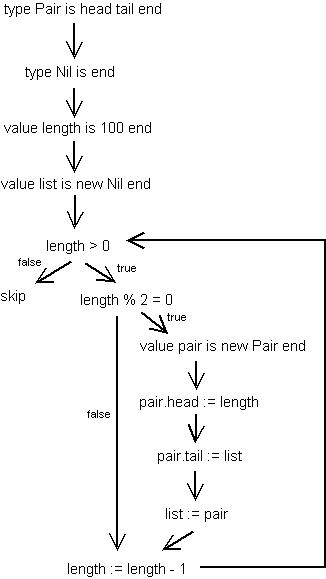
Figure 1shows an example flow graph corresponding to the original example XCom program. Note that a while loop is represented as a test node whose true edge eventually leads back to the test node. XMF provides a packages called Graph that provides a basic collection of graph structures and operations. A graph node is created: Node(l) where l is the label on the graph node. A graph edge is created: Edge(l,s,t) where l is the label on the edge, s is the source node for the edge and t is the target node for the edge. A graph is created: Graph(N,E) where N is a set of nodes and E is a set of edges. The graph shown in figure 1 is constructed as follows where classes Node and Edge have been specialized appropriately:
Graphs provide an operation reduce that takesa node n and a sub-graph H such that G.reduce(n,H) produces a new graph that is the result of removing H from G, adding n to the new graph and re-linking to n any edges left dangling when H is removed.
1 Flow Graph Patterns
Flow graphs can represent the control flow of a wide variety of different languages and are used to analyse the structure of programs. The basic elements of flow graphs are very low level - just nodes (representing statements and expressions) and edges (representing flow between computational states and the outcome of tests).
The low-level nature of flow-graphs gives rise to a weak correspondence language features. This is done by identifying patterns in flow-graphs; wherever the pattern occurs, it can be replaced by a single node. The choice of patterns depends on the collection of program features that we intend to work with. For the purposes of XCom we will capture the following patterns: P is a pair of statements performed in sequence; C is an if statement and W is a while-loop.
The rest of this section shows how the pattern matching facilities of XMF can be used to detect these patterns. We define a flow-graph aspect to XMF graphs by adding reduction operations to the class Graph. The simplest case is detecting and reducing a P node. This occurs when two statements are linked via a next edge. The reduction is shown in figure 2.

A W pattern corresponds to awhile loop and occurs when a test node has a true outcome that is a body statement whose next leads back to the test. The false outcome leads to some root node for the rest of execution. The reduction involves replacing the test and its body with a W node and adding a new next edge from the W node to the root. The reduction is shown in figure 3.

A C pattern corresponds to an if statement and occurs when there isa test node leading to two nodes both of which lead to a single root node. This forms a diamond pattern with the test node at one end. The test, then and else parts of the graph are removed and replaced with a C node. The reduction is shown in figure 4.

Equality on graphs is defined in terms of the labels on the nodesand edges. Two graphs G and H are equal when they have the same number of nodes, when the respective sets of labels are equal, when the edges of G correspond to the edges of H in terms of the source and target nodes and when the respective sets of edge labels are equal.
Graph reduction can involve more than one step. For example, certain configurations of graph require a P reduction to occur before a C reduction can occur. In order to reduce a graph fully we continually perform a reduction until no further reductions can take place:
Appendix A Implementation Issues
1 Working with Files
XMF is a dynamic engine that runs program code loaded from files. Files can be loaded at any time and the definitions come into immediate effect. It is usual for the files to be loaded form the top-level command loop (although loading files from an executing program is also possible). Files have a ’.xmf.’ extension and have a specific format:
The parse imports are used to place syntax classes into scope forthe rest of the file. If a syntax class C is in scope then the file may contain constructs of the form @C … end. When the XMF parser encounters such a construct it looks up the syntax classes in scope, finds a class named C and uses the grammar of C to parse the construct and to synthesize a performable element. Each parse import has the form:
where a path references a name-space containing syntax classes. Typicallya file will contain a single parser-import for the name-space XOCL; this name-space contains all the syntax classes for XOCL definitions such as For, Class, Package, attribute etc.
The imports are used to place named elements in scope for the rest of the file. Each import references a name-space whose named elements can be referenced within the file without further qualification. Each import has the form:
A definition is used to add an element to a container; typically addinga named element to a name-space. A definition has the form:
where the path references a name-space and the expression evaluatesto produce a named element. On loading the file the expression is evaluated, added to the name-space and then initialised (causing any internal references to be resolved). Typically, definitions are used to create class and package definitions.
Definitions are also used to add operations to classes. It is usual to spread the definition of a package and a class over several files, each file contains the definition of various related features. For example a package may be defined in a file, its classes in several files and then the operations for each class in several further files. When doing this, care should be taken to load the files in an appropriate order so that the name-spaces referenced in a definition are available when the file is loaded.
Commands in files are just XOCL expressions terminated by a ’;’. Typically commands are used for their side-effect.
Here is a typical file:
A source file is compiled using the operation:
This operation takes three arguments: the path to the source fileand two boolean values both of which should be true. If the file compiles correctly then the resulting binary file has an extension ’.o’ and can be loaded using String::loadBin(). The top-level command loop has some useful commands that make it easy to compile and load files. The paths are supplied without file extensions:
2 Manifests
XOCL applications tend to run to a number of files. It is possible to write a single file containing directives to compile and load the application files in the correct order, however this becomes difficult to manage since paths have to be absolute etc. The manifest language construct works like a make-file: it is used to list all the files in a module and all the sub-modules. The manifest uses paths relative to a root so that the module is easily relocatable. In addition manifests include some useful directives that can be used to control the compilation and loading of the module.
A manifest file is called Manifest.xmf and has the following structure:
The name of the manifest is just used for documentation. A manifestfile occurs in a directory, all directives in the manifest are relative to this directory. A directive refers either to a file or a directory. A file directive has the following form:
The optional load-time directive specifies when the file should beloaded. A manifest is used to both compile and load files; load-time directives are one of:
CompileTime; RunTime; Both; None. The path to the file is relative to the directory containing the manifest and should be specified with no file extension. Whe the manifest is used to compile entries, a file is compiled if the source (.xmf) is out of date with respect to the binary (.o). Once compiled if the load-time directive is specified as CompileTime or Both then the file is loaded. When the manifest is used to load entries, the binary is loaded providing that the load-time directive is not specified or is RunTime or Both.
A directory directive has the following form:
where the path references a sub-directory that contains a manifestfile. On compilation, the referenced manifest is loaded and its entries compiled. On loading, the referenced manifest is loaded and its entries are loaded.
The following is a typical manifest:
Manifests can be used under program control:
The top-level command loop provides commands that make it easy touse manifests. In the following, ¡PATH¿ refers to a directory containing a manifest file:
3 XMF Startup Arguments
XMF can be started from a batch file or from Java. In both cases initialisation arguments are supplied to the VM as it starts up. These arguments are detailed below. Subsequent sections describe how these arguments are supplied to the different ways of starting XMF.
- •
-arg <NAME>:<VALUE> The global object named xmf contains a collection of name/value pairs that are supplied via this initialzation argument designator. The name and the value are separated using :. The collection of supplied arguments can be referenced as xmf.startupArgs(). Given a name n for an argument, the value is found as xmf.startupArgs()->lookup(n).
- •
-filename <FILE>. Specifies a binary file containing a replacement for the XMF top-level command loop when running the evaluator image (see below). When starting the evaluator image, if this argument designator is supplied then the contents are loaded and executed instead of starting the command loop. When the file completes then the XMF VM terminates.
- •
-heapSize <SIZE>. The size of the XMF heap is set using this initialisation argument designator. The size should be a value in XMF VM words and must be sufficiently large to accommodate any specified image bearing in mind that the Java VM will manage two heaps (for garbage collection) of the specified size. A standard size is 10000.
- •
-initfile <FILE>. When the eval.img image starts (see below) it will, by default, start a top-level command loop. Before the loop starts the supplied binary file is loaded.
- •
-image <FILE>. When the XMF VM starts it loads a saved XMF image into the heap and continues to run the image from the point at which the image was saved. This argument designator specified the file containing the image. For the standard command-line XMF engine, use Images/eval.img.
- •
-port <INT>. Specifies a port that is used by the XMV VM for socket connections.
- •
-stackSize <SIZE>. Specifies the size of the XMF VM stack in machine words. XMF implements tail calling, so it is not usually necessary to specify this argument designator.
A minimal startup is:
4 Starting XMF using a Batch File
There is an example startup file bin/xos.bat for starting the XMF VM with the top-level command loop defined in eval.img. Run this supplying the value of XMFHOME to start a top-level command loop:
or by supplying a filename to replace the top-level loop:
5 Starting XMF from Java
The XMF VM can be started from Java as follows:
Different combinations of arguments can be supplied as required.
6 Rebuilding XMF
Rebuilding XMF is in two stages (for mainly historical reasons). Assuming you have all the binaries recompiled (see the next section):
The above creates a new image in XMFHOME\Images\xmf.img.This is a basic image that supports XOCL etc. The next step extends this image by loading libraries most of which are essential to run the top-level command loop:
A fresh XMFHOME\Images\eval.img is created.
7 Recompiling XMF
XMF can be recompiled only from a valid XMF top-level command loop which requires a valid eval.img. This is done as follows:
If you modify the XMF sources in any way then you will need to recompileand the rebuild to create a fresh image. The rebuilsing process is describes in the previous section.
8 Debugging
Operations can be traced so that information is printed out when the operation is entered and when it is exited. The output is intended to reflect the call nesting. Use Operation::trace() to set tracing and Operation::untrace() to remove tracing. Use Container::traceAll() to trace all operations in a name-space and Container::untraceAll() to remove all tracing.
9 Boolean Operations
The following list shows the main operations defined by the datatype Boolean:
10 Float Operations
The following list shows the main operations defined by the datatype Float:
11 Integer Operations
The following list shows the main operations defined by the datatype Integer:
12 Sequence Operations
The following list shows the main operations defined by the datatype Seq(Element):
13 Set Operations
The following list shows themain operations defined by the datatype Set(Element):
14 String Operations
The following list shows the main operations defined by the datatype String:
15 OCL Syntax Classes
This section defines the classes that make up the Object Command Language (the core part of XOCL). They are defined in the package OCL. The syntax classes are grouped roughly in terms of their basic properties and usage.

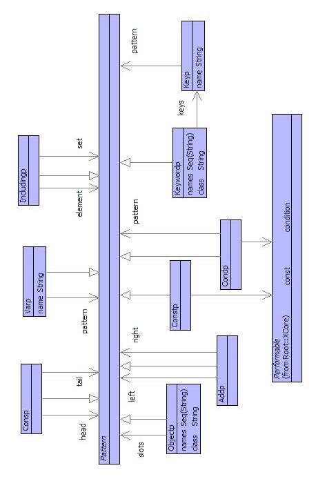
Figure 1 shows classes for atomic expressions. Figure 2 shows the classes for patterns that occur in argument positions of operation expressions (and in @Case expressions). Briefly, Consp is a pair pattern, Varp is a simple variable, Includingp is a set pattern, Objectp is a pattern corresponding to a constructor, Addp is a sequence concatenation or set union pattern, Constp is a constant (where the constant is the result of evaluating an expression), Condp is a guard and Keywordp is a pattern matching objects where the slots are given as keys.


Figure 3 shows the syntax of let-expressions. Figure 4 shows the classes for iteration expressions. Both set and sequence expressions are represented as instances of SetExp with the collType set to Set or Seq respectively. A CollExp supports all concrete expressions of the form S->x(a,b,c) and S->x where the arguments to the latter default to the empty sequence. IterExp represents all concrete expressions of the form S->n(x | e) where n is exists, forAll, select, collect or reject.


Figure 5 shows the classes for operations. Note that operation arguments are not shown but are an attribute of type Seq(Pattern). Figure6 shows the classes for update expressions. Updates can be variable, x := e, path P::Q::x := e, or head and tail: s->head := e and s->tail := e.

Figure 7 shows the rest of the expression types.