Transition fronts and stretching phenomena for a general class of reaction-dispersion equations
Abstract
We consider a general form of reaction-dispersion equations with non-local dispersal and local reaction. Under some general conditions, we prove the non-existence of transition fronts, as well as some stretching properties at large time for the solutions of the Cauchy problem. These conditions are satisfied in particular when the reaction is monostable and when the dispersal operator is either the fractional Laplacian, a convolution operator with a fat-tailed kernel or a nonlinear fast diffusion operator.
Dedicated to the memory of Professor Paul Fife
1 Introduction
This note is concerned with fast propagation phenomena and large time qualitative properties of dispersion-reaction equations of the type
| (1.1) |
The given reaction function is of class and such that . Throughout the paper, we assume that, for any , the Cauchy problem
| (1.2) |
admits a unique mild solution, such that for every and is uniformly continuous with respect to in for every . The equation (1.1) is assumed to be autonomous in the sense that, for any solution of the Cauchy problem (1.2) and for any , the function solves (1.2) with initial condition . We also assume that a comparison principle holds for (1.2), that is, for any two solutions and with respective initial conditions and ,
| (1.3) |
Lastly, the solutions of (1.2) are assumed to have infinite spreading speeds (to the right) in the sense that
| (1.4) |
The first typical example of equations (1.1) for which these conditions are fulfilled is the monostable reaction-diffusion equation with fractional diffusion
| (1.5) |
where the reaction function is monostable, that is
| (1.6) |
and the dispersal operator is the fractional Laplacian with , see [6] (see also [5] for similar equations in periodic media). In [6], the function is also assumed to be concave in , but the condition (1.4) actually holds under the condition (1.6) by the comparison principle and putting below a concave function on the interval , with as small as wanted. The set of functions satisfying (1.6) includes the class of Fisher-KPP [20, 29] nonlinearities for which, in addition to these assumptions, satisfies in . It also contains the set of concave functions with and on , whose archetype is the logistic nonlinearity .
A second important class consists of integro-differential equations with fat-tailed dispersal kernels
| (1.7) |
where is of the type (1.6) and the dispersal operator is a convolution operator
with a fat-tailed positive even kernel such that
see [21]. Notice that such kernels are called “fat tailed” since they decay slowly as in the sense that as for every . Archetypes are with , and some normalization constant , or with and some . Such operators and equations arise in many physical or ecological models, see e.g. [10, 17, 18, 19, 30, 31, 32, 36].
Lastly, the conditions (1.3) and (1.4) are also fulfilled when the dispersal operator corresponds to fast nonlinear diffusion. Using a detailed formal analysis of the equation
| (1.8) |
with and where satisfies (1.6), it was shown in [28] that the assumption (1.4) was fulfilled. In [46], this result was extended to the case of nonlinear fractional diffusion equations:
| (1.9) |
with and and where satisfies (1.6) and is a concave function. Due to the comparison principle (1.3), which is valid for both (1.8) and (1.9), it can be shown that the condition (1.4) holds without the concavity assumption, as for the standard fractional Laplacian.
Given the few general assumptions (1.3) and (1.4), the goal of the paper is twofold. Firstly, we will prove the non-existence of front-like entire solutions. Secondly, further stretching properties of the solutions of the Cauchy problem (1.2) at large time will be shown. As a corollary of the second main theorem, we will show that the solutions of (1.2) are in some sense flat at some large times in left and right neighborhoods of any level set. We again insist on the fact that these results will hold for the four main examples (1.5), (1.7), (1.8) and (1.9).
2 Non-existence of transition fronts
When propagating solutions are mentioned, one immediately has in mind standard traveling fronts , with velocity and front profile such that and . On the one hand, without the assumption (1.4), standard traveling fronts are known to exist when we consider equations (1.8) with the standard (local) Laplacian or a nonlocal convolution operator with thin-tailed dispersal kernel which is nonnegative even and exponentially bounded in the sense that and for some . More precisely, when is of the type (1.6), these fronts exist for every speed , with a positive minimal speed . Furthermore, uniqueness of the profile and stability results for a given have been shown, with possibly heterogeneous nonlinearities , see [1, 7, 12, 13, 15, 16, 29, 41, 42, 44, 45, 47]. However, even for the reaction-diffusion equation with local diffusion and of the type (1.6), fast propagation phenomena with infinite spreading speed as in (1.4) is known to occur when decays to as more slowly than any exponentially decaying function, see [25]. On the other hand, some existence, uniqueness and stability results of standard traveling fronts have also been shown for some nonlocal equations of the type (1.1) with fractional Laplacians or fat-tailed dispersal convolution kernels , but for other types of nonlinearities or than (1.6), see e.g. [2, 8, 9, 12, 14, 15, 16, 22, 23, 35].
Here, the assumptions (1.3) and (1.4) forbid standard traveling fronts to exist, since all non-trivial solutions of the Cauchy problem accelerate with infinite speed as in the sense of (1.4). This non-existence result has already been known in the case of the fractional Laplacian [6, 22] as well as in the convolution case with non-exponentially-bounded kernels [21, 48]. Non-existence of standard traveling fronts has also been derived for the fast nonlinear diffusion equations (1.8) and (1.9) [28, 46]. However, other propagating solutions connecting and , more general than the standard traveling fronts, can be investigated. These solutions, called transition fronts, have been defined in [3, 4] in more general situations. In the one-dimensional situation considered here, as a wave-like solution defined in [43], the following definition holds.
Definition 2.1 (Transition front)
The real numbers therefore reflect the positions of a transition front as a function of time. However, the ’s are not uniquely defined since any family satisfies (2.1) as soon as does and remains bounded. Roughly speaking, condition (2.1) means that the diameter of the transition zone between the sets where and is uniformly bounded in time in the sense that, for every , there is a nonnegative real number such that, for all ,
up to a negligible set. Transition fronts connecting on the left and on the right can be defined similarly by permuting the limits as in (2.1). We will therefore only consider here transition fronts connecting on the right and on the left. Obviously, any standard traveling front with and would be a transition front connecting and with , but, as already emphasized, the assumption (1.4) excludes the existence of standard traveling fronts for (1.1). Nevertheless, transition fronts can a priori be much more general than standard traveling fronts, since no assumption is made on the family of front positions . In particular, transition fronts different from the standard traveling fronts have been constructed recently for some homogeneous or heterogeneous local reaction-diffusion equations [26, 27, 33, 34, 37, 38, 39, 49, 50], and fronts with global speed having different limits as are also known to exist even for the homogeneous local Fisher-KPP reaction-diffusion equation [24, 26, 49]. For our equation (1.1), transition fronts with global speed growing arbitrarily as are a priori not excluded.
Our first result shows actually that this is anyway impossible, since transition fronts cannot exist whatever the family of positions may be.
Theorem 2.2
Theorem 2.2 generalizes the known non-existence result of standard traveling fronts for the equations of the type (1.5) with the fractional Laplacian, (1.7) with a fat-tailed dispersal kernel ,and (1.8) and (1.9) with fast nonlinear diffusion since the standard fronts are particular classes of transition fronts.
Roughly speaking, this non-existence result can be heuristically explained as follows: for any transition transition front connecting and , the uniformity (with respect to time) of the limits (2.1) prevents the front from traveling too fast (see also [26] for a similar phenomenon for local reaction-diffusion equations), and this last property is finally in contradiction with the spreading properties (1.4) combined with the comparison principle (1.3).
Proof of Theorem 2.2. We argue by contradiction. So assume that, under the assumptions (1.3) and (1.4), equation (1.1) admits a transition front connecting and . Let be a family of real numbers such that (2.1) holds.
For every , denote
and
It follows from (2.1) that are real numbers. The definitions of imply that
| (2.2) |
and
| (2.3) |
together with . Property (2.1) also yields
Indeed, otherwise, there would exist a sequence of real numbers such that
whence as , contradicting the property
Similarly, there holds
Eventually, using again , one infers that the families and are all bounded.
From the general regularity assumptions made in the paper, the function is actually uniformly continuous with respect to in , for every . By considering , it follows in particular that there exists such that, for all , and ,
As a consequence, for every , denoting the non-negligible measurable sets defined as
it follows that
| (2.4) |
On the other hand, from (2.1), there is such that, for every ,
Since, for every , the sets have a positive measure, one infers from (2.4) that
and
Remembering that the quantities are bounded, one gets that
| (2.5) |
Finally, notice that a.e. in by (2.2), where denotes the characteristic function of a measurable set . The comparison principle (1.3) implies that, for every ,
where denotes the solution of the Cauchy problem (1.2) with initial condition . It follows then from the spreading property (1.4) that as for every , whence
For any given , property (2.3) then yields for all large enough, whence . Therefore,
since is bounded. As a conclusion, as , which contradicts (2.5). The proof of Theorem 2.2 is thereby complete.
3 Stretching at large time for the Cauchy problem (1.2)
The second main result is concerned with flattening and stretching properties at large time for the solutions of the Cauchy problem (1.2). We assume in this section that the equation (1.1) is homogeneous, in the sense that, for any and for any , there holds
| (3.1) |
where and denote the solutions of the Cauchy problem (1.2) with initial conditions and . The property (3.1) is satisfied by the previous examples of dispersal operators : fractional Laplacian , the convolution operator , the nonlinear fast diffusion and the nonlinear fractional diffusion . If follows from assumptions (1.3) and (3.1) that if is nonincreasing, then
whence a.e. in for every . In other words, is nonincreasing for every . Under these conditions, for every , denote
and
and observe that . Lastly, for every , set
| (3.2) |
Notice that if , while if . Moreover,
Theorem 3.1
Theorem 3.1 means that the function becomes regularly as stretched as wanted as , that is, for any given , the “reaction” zone where ranges between and cannot stay bounded at large time. However, the following reasonable conjecture remains open:
Conjecture 3.2
Under the assumptions of Theorem 3.1, as for any .
The assumptions and are satisfied for instance if with , , with , and with and , and if and (remember that the function is such that ). These conditions are also satisfied for the same type of dispersal in the case , with on .
Theorem 3.1 is in spirit similar to a result obtained in [25] for the solutions of the Cauchy problem of the equation : if satisfies (1.6) and is non-increasing over and if the initial condition satisfies , , together with for every and for some and , then as . This last conclusion is clearly stronger than (3.3). But, for our equation (1.1), we make weaker regularity assumptions on . In particular, may well be discontinuous and, since there is in general no spatial regularizing effect for (1.1), may not be differentiable or even continuous. But the property (3.3) still gives some information about the profile of at large time. In particular, even if may be discontinuous at some points, the discontinuity jumps cannot stay large as time goes to .
Moreover, we can describe the profile of the solution around the position of each level sets. More precisely, for any level , becomes regularly as flat as wanted at large times and becomes as close as wanted to locally on the left and on the right of the position .
Corollary 3.3
Under the same assumptions as in Theorem 3.1, for every and there holds
| (3.4) |
Proof of Theorem 3.1. Let be a solution of the Cauchy problem (1.2) with a nonincreasing initial condition . As already emphasized, is nonincreasing in for every . In particular, if , then defined in (3.2) is a real number and
| (3.5) |
Let now and be two given real numbers such that and assume by contradiction that , that is, there exist and such that
| (3.6) |
Since and as , one can assume without loss of generality that for all , whence and are real numbers for . Notice that
| (3.7) |
From the uniform continuity of with respect to in , there is such that, for every ,
Now, for every , one has a.e. in , whence
whereas a.e. in and
Since , one infers from the definition of that
whence
| (3.8) |
On the other hand, since is nonincreasing and ranges in , it follows again from the definition of that
Therefore, the comparison principle (1.3) implies that, for every , a.e. in , where denotes the solution of the Cauchy problem (1.2) with initial condition . The assumption (1.4) applied to therefore yields as for every , whence
Finally, for any arbitrary positive real number , there holds
for large enough, whence for large enough, since is nonincreasing. As a consequence,
and, since is arbitrary, it follows that as . This contradicts (3.8) and the proof of Theorem 3.1 is thereby complete.
Remark 3.4
Consider here the case of equation (1.5) with the fractional Laplacian with . For this equation, there is a regularizing effect in the spatial variable and, under the assumptions of Theorem 3.1, it follows that the solution is of class in for every , with bounded derivatives with respect to and . For any given , there is a real number such that, for every , there is a unique such that . We now claim that
Indeed, otherwise, there are and such that for all . It follows then from the implicit function theorem that the function is of class and that
for all . Therefore, there is such that for all and one can get a contradiction as in the end of the proof of Theorem 3.1.
Again for (1.5) with the fractional Laplacian , and with a Fisher-KPP function , Roquejoffre and Tarfulea [40] recently showed that the partial derivatives of with respect to are all bounded by times an exponentially decaying function, that is, for every , there are positive constants and such that for large . This result has been proved under the additional condition that is exponentially decaying as , and it actually holds in any spatial dimension. It implies in particular that as . Moreover, it is proved in [40] that the large time dynamics of the KPP problem (1.5) is in some sense the same as that of the ODE
More generally speaking, under the general conditions (1.3), (1.4) and (3.1), we conjecture that fast propagation should lead to a flattening of the solution in the sense that, at least if on , then the only -monotone solutions of (1.5) are actually -independent, that is, they can be written as , where for all with and .
An intermediate result that we prove here under the sole conditions (1.3), (1.4) and (3.1) is the flattening result stated in Corollary 3.3. We point out that this result holds for all equations (1.5), (1.7), (1.8) and (1.9) under the same conditions as in Section 1.
Proof of Corollary 3.3. Let be a solution of the Cauchy problem (1.2) with a nonincreasing initial condition . As already emphasized, is nonincreasing in for every . In particular, if , then defined in (3.2) is a real number and (3.5) holds.
Let then be any real number such that be any positive real number and be any positive real number such that . From Theorem 3.1, there exist two increasing sequences and of positive real numbers such that
As a consequence, there exists such that, for all ,
Thus, by (3.5) applied with , and , one infers that, for all ,
whence
for all . Since can be arbitrarily small and , the proof of Corollary 3.3 is thereby complete.
Remark 3.5
It easily follows from the proof of Corollary 3.3 that, if Conjecture 3.2 is true, then for any level the solution of the Cauchy problem (1.2) converges to locally around each position of the level set as , that is,
for every . This last convergence result would then hold automatically for the whole family and on both the left and right of simultaneously.
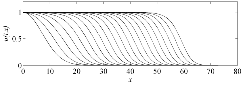
Lastly, in order to illustrate the theoretical results on the flattening and stretching properties of the solutions of the Cauchy problem (1.2), we have performed some numerical simulations that are depicted in figures 1 and 2. They have been done with the KPP nonlinearity for the three examples with , with , and with (Fig.1, a, b and c, respectively). These properties, and the acceleration of the solutions in each of these three cases are to be compared with the well-known convergence to a standard travelling front which can be observed with the standard diffusion operator (Fig. 1, d). To compute these solutions, we used (a and b): the Strang splitting, which consists in splitting the equation (1.2) into two simpler evolution problems [11]: and which are treated with fast Fourier transform techniques and which solution can be computed explicitly; (c and d): the time-dependent finite element solver of Comsol Multiphysics©.

References
- [1] D.G. Aronson, H.F. Weinberger, Multidimensional nonlinear diffusions arising in population genetics, Adv. Math. 30 (1978), 33-76.
- [2] P.W. Bates, P.C. Fife, X. Ren, X. Wang, Traveling waves in a convolution model for phase transitions, Arch. Ration. Mech. Anal. 138 (1997), 105-136.
- [3] H. Berestycki, F. Hamel, Generalized travelling waves for reaction-diffusion equations, In: Perspectives in Nonlinear Partial Differential Equations. In honor of H. Brezis, Amer. Math. Soc., Contemp. Math. 446, 2007, 101-123.
- [4] H. Berestycki, F. Hamel, Generalized transition waves and their properties, Comm. Pure Appl. Math. 65 (2012), 592-648.
- [5] X. Cabré, A.-C. Coulon, J.-M. Roquejoffre, Propagation in Fisher-KPP type equations with fractional diffusion in periodic media, C. R. Math. Acad. Sci. Paris 350 (2012), 885-890.
- [6] X. Cabré, J.-M. Roquejoffre, The influence of fractional diffusion in Fisher-KPP equations, Comm. Math. Phys. 320 (2013), 679-722.
- [7] J. Carr, A. Chmaj, Uniqueness of travelling waves for nonlocal monostable equations Proc. Am. Math. Soc. 132 (2004), 2433-2439.
- [8] X. Chen, Existence, uniqueness, and asymptotic stability of traveling waves in nonlocal evolution equations, Adv. Diff. Equations 2 (1997), 125-160.
- [9] A. Chmaj, Existence of traveling waves in the fractional bistable equation, Arch. Math. 100 (2013), 473-480.
- [10] J. S. Clark, Why trees migrate so fast: Confronting theory with dispersal biology and the paleorecord, Am. Nat. 152 (1998), 204-224.
- [11] A.-C. Coulon, Propagation in reaction-diffusion equations with fractional diffusion, PhD Thesis, Institut de Mathématiques de Toulouse and Universitat Politècnica de Catalunya (2014).
- [12] J. Coville, On uniqueness and monotonicity of solutions of non-local reaction diffusion equation, Ann. Mat. Pura Appl. 185 (2006), 461-485.
- [13] J. Coville, J. Dávila, S. Martínez, Non-local anisotropic dispersal with monostable nonlinearity, J. Diff. Equations 244 (2008), 3080-3118.
- [14] J. Coville, J. Dávila, S. Martínez, Pulsating fronts for nonlocal dispersion and KPP nonlinearity, Ann. Inst. H. Poincaré, Anal. Non Linéaire 30 (2013), 179-223.
- [15] J. Coville, L. Dupaigne, Propagation speed of travelling fronts in non local reaction-diffusion equations, Nonlinear Anal. 60 (2005), 797-819.
- [16] J. Coville, L. Dupaigne, On a nonlocal reaction diffusion equation arising in population dynamics, Proc. Roy. Soc. Edinburgh A 137 (2007), 727-755.
- [17] D. del-Castillo-Negrete, Truncation effects in superdiffusive front propagation with Lévy flights, Phys. Rev. 79 (2009), 1-10.
- [18] D. del-Castillo-Negrete, B.A. Carreras, V. Lynch, Front propagation and segregation in a reaction-diffusion model with cross-diffusion, Phys. D 168/169 (2002), 45-60.
- [19] P. C. Fife, Mathematical Aspects of Reacting and Diffusing Systems, Lecture Notes in Biomath. 28, Springer-Verlag, Berlin, New York, 1979.
- [20] R.A. Fisher, The advance of advantageous genes, Ann. Eugenics 7 (1937), 335-369.
- [21] J. Garnier, Fast propagation in integro-differential equations, SIAM J. Math. Anal. 43 (2011), 1955-1974.
- [22] C. Gui, T. Huan, Traveling wave solutions to some reaction diffusion equations with fractional Laplacians, preprint.
- [23] C. Gui, M. Zhao, Traveling wave solutions of Allen-Cahn equation with a fractional Laplacian, Ann. Institut H. Poincaré Anal. Non Linéaire, forthcoming.
- [24] F. Hamel, N. Nadirashvili, Travelling waves and entire solutions of the Fisher-KPP equation in , Arch. Ration. Mech. Anal. 157 (2001), 91-163.
- [25] F. Hamel, L. Roques, Fast propagation for KPP equations with slowly decaying initial conditions, J. Diff. Equations 249 (2010), 1726-1745.
- [26] F. Hamel, L. Rossi, Transition fronts for the Fisher-KPP equation, Trans. Amer. Math. Soc., forthcoming.
- [27] F. Hamel, L. Rossi, Admissible speeds of transition fronts for non-autonomous monostable equations, preprint.
- [28] J. R. King, P. M. McCabe, On the Fisher-KPP equation with fast nonlinear diffusion, Proc. R. Soc. A 459 (2003), 2529-2546.
- [29] A.N. Kolmogorov, I.G. Petrovsky, N.S. Piskunov, Étude de l’équation de la diffusion avec croissance de la quantité de matière et son application à un problème biologique, Bull. Univ. Etat Moscou, Série Intern. A 1 (1937), 1-26.
- [30] M. Kot, M. Lewis, P. Van den Driessche, Dispersal data and the spread of invading organisms, Ecology 77 (1996), 2027-2042.
- [31] R. Mancinelli, D. Vergni, A. Vulpiani, Front propagation in reactive systems with anomalous diffusion, Phys. D 185 (2003), 175-195.
- [32] J. Medlock, M. Kot, Spreading disease: Integro-differential equations old and new, Math. Biosci. 184 (2003), 201-222.
- [33] A. Mellet, J. Nolen, J.-M. Roquejoffre, L. Ryzhik, Stability of generalized transition fronts, Comm. Part. Diff. Equations 34 (2009), 521-552.
- [34] A. Mellet, J.-M. Roquejoffre, Y. Sire, Generalized fronts for one-dimensional reaction-diffusion equations, Disc. Cont. Dyn. Syst. A 26 (2010), 303-312.
- [35] A. Mellet, J.-M. Roquejoffre, Y. Sire, Existence and asymptotics of fronts in non local combustion models, Comm. Math. Sci. 12 (2014), 1-11.
- [36] D. Mollison, Spatial contact models for ecological and epidemic spread, J. R. Stat. Ser. B Stat. Methodol. 39 (1977),283-326.
- [37] G. Nadin, L. Rossi, Propagation phenomena for time heterogeneous KPP reaction-diffusion equations, J. Math. Pures Appl. 98 (2012), 633-653.
- [38] J. Nolen, J.-M. Roquejoffre, L. Ryzhik, A. Zlatoš, Existence and non-existence of Fisher-KPP transition fronts, Arch. Ration. Mech. Anal. 203 (2012), 217-246.
- [39] J. Nolen, L. Ryzhik, Traveling waves in a one-dimensional heterogeneous medium, Ann. Inst. H. Poincaré, Analyse Non Linéaire 26 (2009), 1021-1047.
- [40] J.-M. Roquejoffre, A. Tarfulea, Gradient estimates and symmetrization for Fisher–KPP front propagation with fractional diffusion, preprint.
- [41] D.H. Sattinger, Weighted norms for the stability of traveling waves, J. Diff. Equations 25 (1977), 130-144.
- [42] K. Schumacher, Travelling-front solutions for integro-differential equations. I., J. Reine Angew. Math. 316 (1980), 54-70.
- [43] W. Shen, Traveling waves in diffusive random media, J. Dyn. Diff. Equations 16 (2004), 1011-1060.
- [44] W. Shen, A. Zhang, Spreading speeds for monostable equations with nonlocal dispersal in space periodic habitats. J. Diff. Equations 249 (2010), 747-795.
- [45] W. Shen, A. Zhang, Traveling wave solutions of spatially periodic nonlocal monostable equations, Comm. Appl. Nonlinear Anal. 19 (2012), 73-101.
- [46] D. Stan, J. L. Vázquez, The Fisher-KPP equation with nonlinear fractional diffusion, SIAM J. Math. Anal. 46 (2014), 3241-3276.
- [47] K. Uchiyama, The behavior of solutions of some semilinear diffusion equation for large time, J. Math. Kyoto Univ. 18 (1978), 453-508.
- [48] H. Yagisita, Existence and nonexistence of traveling waves for a nonlocal monostable equation, Publ. RIMS Kyoto Univ. 45 (2009), 925-953.
- [49] A. Zlatoš, Transition fronts in inhomogeneous Fisher-KPP reaction-diffusion equations, J. Math. Pures Appl. 98 (2012), 89-102.
- [50] A. Zlatoš, Generalized traveling waves in disordered media: existence, uniqueness, and stability, Arch. Ration. Mech. Anal. 208 (2013), 447-480.