A Topological Approach to Spectral Clustering

1. Introduction

The analysis of complex, high-dimensional data is one of the major research challenges in contemporary computer science and statistics. In recent years, geometric and topological approaches to data analysis have been shown to yield important insights into the structure of complex data sets. The common point of departure in these methods is the assumption that data in high-dimensional spaces is often concentrated around a low-dimensional manifold or other topological space.

Geometric techniques, in particular, have proven to be particularly successful. These have largely concentrated on approximating the local geometry of the data as a step towards non-linear dimension reduction. Once an embedding of the data in a lower-dimensional space has been found, standard statistical techniques are then used to analyze the data in the lower-dimension. Methods in this class include ISOMAP [8], Locally Linear Embedding [10], Hessian Eigenmaps [6], Laplacian Eigenmaps [1], and Diffusion Maps [5]. Most of these techniques build a weighted graph to approximate the Laplace-Beltrami operator on a manifold, or else a related Markov chain on a graph, and then use the eigenvalues and eigenvectors of the resulting operator to reduce the dimension of the data, often, in practice, followed by the application of a $k$ -means clustering algorithm to perform the clustering of the data [12], [11]. We encounter a more topologically-oriented approach in [3], in which persistent homology [13, 7, 2] is used to help a statistician identify high-density regions of a distribution function.

In this article, we give an algorithm that directly uses the topological information in the graph Laplacian to produce a clustering of the data, eliminating the need for separate dimension reduction and clustering steps. This process, furthermore, illustrates the utility of considering the data clustering problem from a topological, instead of purely analytic, perpective, i.e. to consider clustering as a problem of estimating the number of connected components of the support of an idealized underlying distribution. While the topological aspect of the clustering problem has been generally acknowledged in the topological data analysis community for some time, this is, to the best of our knowledge, the first completely data-driven clustering algorithm that explicitly exploits this point of view. Additionally, the algorithm produces both the number of clusters and the clusters themselves with no additional information required, unlike popular algorithms such as $k$ -means clustering or $k$ -nearest-neighbor clustering, in which the number of clusters or other additional input is required. Finally, we propose what we believe to be the first geometric and information-theoretic model selection criteria for choosing a Laplacian (or, more precisely, the associated Markov process) from a family of candidates built from the geometric properties of the sample space alone, instead of from observations of the Markov process.

2. Topology and Clustering

In all that follows, we will assume that there is an ideal unknown probability distribution $P(X)$ supported on a disconnected metric space $X=\sqcup_{i=1}^{k}X_{i}$ , where $X$ is embedded as a (possibly much lower dimensional) subset of an ambient space $Y$ . We will further suppose that the distribution $P(X)$ may be corrupted by noise, and that the coordinates of the sample points are given by sampling from the combined noisy distribution. We will consider a clustering to be correct if it accurately recovers the number of connected components of $X$ and it assigns to each sample point to the nearest connected component.

When $X$ has the homotopy type of a finite CW-complex, the number of connected components of $X$ is given by the dimension of the $0$ -th real cohomology group $H^{0}(X;\mathbb{R})$ . Furthermore, if $X$ is a manifold, this is equal to the dimension of the kernel of the Laplace-Beltrami operator $\Delta_{X}$ through a small amount of Hodge theory [9]. We recall that the Laplace-Beltrami operator $\Delta:L^{2}(X)\to L^{2}(X)$ may be defined by $\Delta=-d^{*}d$ , where $d$ is the exterior derivative, extended continuously to $L^{2}(X)$ , and $d^{*}$ is its adjoint in $L^{2}(X)$ . It follows, too, that the functions in the kernel are constant on each connected component of $X$ (Lemma 3.3.5 in [9]).

The following proposition now follows easily.

Proposition 2.1.

Let $(X,g)$ be a smooth Riemannian manifold, and let $k$ denote the number of connected components of $M$ . Let $\{\psi_{i}\}_{i=1}^{k}$ be a basis of the kernel of the Laplace-Beltrami operator $\Delta_{X}$ of $X$ , and define the map $\Psi:X\to\mathbb{R}^{k}$ by

\Psi(x)\mathrel{\mathchoice{\vbox{\hbox{$\displaystyle:$}}}{\vbox{\hbox{$\textstyle:$}}}{\vbox{\hbox{$\scriptstyle:$}}}{\vbox{\hbox{$\scriptscriptstyle:$}}}{=}}(\psi_{1}(x),\dots,\psi_{k}(x))\in\mathbb{R}^{k}.

Then the image of $\Psi$ consists of exactly $k$ points in $\mathbb{R}^{k}$ , and the image of each connected component of $X$ is a single point.

Proof.

First, we know from [9], Section 3.3, that each basis function $\psi_{i}$ is constant on each connected component of $X$ , and it follows that each connected component is sent to a single point. It only remains to show that no two connected components are sent to the same point. Consider the matrix $A$ defined by $a_{ij}=\psi_{i}(X_{j})$ . Since the $\psi_{i}$ are linearly independent, this is a $k\times k$ matrix of full rank. Suppose now that there are two connected components, $X_{1}$ and $X_{2}$ , whose image under $F$ is the same point $x\in\mathbb{R}^{k}$ . Then two rows of $A$ are the same, and the $\text{rank }A<k$ , a contradiction. Therefore, all of the connected components of $X$ are sent to different points in $\mathbb{R}^{k}$ . ∎

Remark 2.2.

We note, too, that Proposition 2.1 also hold for graphs and the graph Laplacian instead of manifolds, with a nearly identical proof.

3. The Graph Laplacian and the Graph Heat Semigroup

Given a noisy sample from a disconnected metric space $X$ , motivated by the above discussion, our primary task in the clustering problem will be to compute an empirical Laplacian $\hat{\Delta}$ and the corresponding empirical function $\hat{\Psi}$ so that $\hat{\Psi}$ is constant on the points sampled from a given connected component of $X$ . We begin by recalling the construction of the graph Laplacian, the associated heat semigroup, and several fundamental results.

Let $G=(V,E,w)$ be a weighted graph, where the weight function $w:E\to[0,\infty)$ gives the weights of every edge. We define the matrix $L_{G}$ to be

(3.1)

(L_{G})_{(i,j)}=\begin{cases}w(x_{i},x_{j})&i\neq j,\\ -\sum_{v_{j}\in V}w(x_{i},x_{j})&i=j,\\ \end{cases}

where $x_{i},x_{j}\in V$ . We likewise define the corresponding heat operators $e^{-tL_{G}}$ by

e^{-tL_{G}}=\sum_{k=0}^{\infty}\frac{(-tL_{G})^{k}}{k!}.

for $t\in[0,\infty)$ . Note that $e^{-tL_{G}}e^{-sL_{G}}=e^{-(t+s)L_{G}}$ , so the set of matrices $\{e^{-tL_{G}}\}_{t\in[0,\infty)}$ forms a semigroup under matrix multiplication, which we call the graph heat semigroup, or the heat semigroup of G. The following result is immediate from the definitions.

Proposition 3.1.

The vector $v\in\mathbb{R}^{|V|}$ is an eigenvector of $L_{G}$ with eigenvalue $\lambda$ iff $v$ is an eigenvector of $e^{-tL_{G}}$ with eigenvalue $e^{-t\lambda}$ .

As in the manifold case, we have the following result.

Theorem 3.2 ([4], Lemma 1.7.iv, and page 3, equation 1.1).

The number of connected components of $G$ is equal to the dimension of the kernel of $L_{G}$ , and the vectors $v\in\ker L_{G}$ are constant on each connected component of $G$ , i.e. if the vertices $x_{i},x_{j}\in V$ are in the same connected component of $G$ , then for the corresponding coordinates $v$ we have $v_{i}=v_{j}$ .

Remark.

Combining Proposition 3.1 with Theorem 3.2, we see that the dimension of the $1$ -eigenspace of $e^{-tL_{G}}$ is also equal to the number of connected components of $G$ , for any $t\in(0,\infty)$ .

4. Graph Models and Model Selection for the Graph Heat Semigroup

We now describe how to combine the above ideas with several additional observations to perform unsupervised distance-based clustering on a data set $Z$ .

Definition 4.1.

Let $Z$ be a collection of points in a metric space $Y$ . For each $r\geq 0$ , we define a graph $G_{r}=(V_{r},E_{r})$ by

	$\displaystyle V_{r}$	$\displaystyle=Z$
	$\displaystyle E_{r}$	$\displaystyle=\{(x_{i},x_{j})\in Z\times Z\mid d_{Y}(x_{i},x_{j})\leq r\}.$

That is, the vertices for each graph $G_{r}$ are the points in the data set $Z$ , and two vertices in $G_{r}$ are joined by an edge iff the distance between them is at most $r$ .

Once we have a collection of graph models $\{G_{r}\}_{r\geq 0}$ for the data set $Z$ , we compute their corresponding graph Laplacians $L_{G_{r}}$ (which we abbreviate to $L_{r}$ ), and the heat semigroups $\{e^{-tL_{r}}\}_{t\in[0,\infty)}$ . We would now like choose a value $\hat{r}$ from among the $r\geq 0$ so that $\{e^{-tL_{\hat{r}}}\}_{t\in[0,\infty)}$ best represents the heat semigroup $\{e^{-t\Delta_{X}}\}_{t\in[0,\infty)}$ , where $X$ is the support of the distribution of the process which generated the points. To solve the clustering problem, it is sufficient to choose a $\hat{r}$ so that the dimensions of the kernels of $L_{\hat{r}}$ and $\Delta_{X}$ are equal, i.e. so that the graph $G_{\hat{r}}$ has the same number of connected components as $X$ , and then assign each vertex to the correct connected component. Note that, if we choose $r$ too small, then there will be too many small connected components, but if we choose $r$ too large, then there will be too few large ones.

We give two techniques for solving this problem, the first based on a geometric criterion, and the second based on an information-theoretic one. We compare their performance in Section 6.

4.1. Model Selection by Average Relative Neighborhood Volume

Let $M$ be a disconnected closed manifold (i.e. without boundary), let $x\in M$ be a point in $M$ , and denote by $M_{x}\subset M$ the connected component of $M$ containing $x$ . Let $|A|$ denote the volume of $A$ for any $A\subset M$ using the volume form on $M$ . Our first technique for choosing $r$ is based on the observation that, on any disconnected manifold $M$ , where each connected component is of dimension $>0$ , for any point $x\in M$ , the function

R(x)\coloneqq\lim_{U\in\mathcal{N}(x)}\frac{|U|}{|M_{x}|}=0

where the limit is taken over the net defined by the partially ordered set $\mathcal{N}(x)$ of neighborhoods of $x$ . That is, for any $x\in M$ , the ratio of the volume of a neighborhood of $x$ to the volume of the connected component containing $x$ may be made arbitrarily small. It follows that

R_{M}\coloneqq\frac{1}{|M|}\int_{M}R(x)\,dx=0

as well.

Now consider the family of graphs $G_{r}$ built on a fixed, finite sample of points $Z$ taken from a uniform distribution on a metric space $X$ as in Definition 4.1. We say that a subset $U\subset V_{r}=Z$ is a neighborhood of a vertex $x\in Z$ iff $U$ contains $x$ and all vertices adjacent to $x$ , and let the volume of a subset of $V_{r}$ equal its cardinality. Note that the volume of any neighborhoods $U$ of a point $x$ is necessarily bounded below by $1$ , and furthermore, if $M_{x}=\{x\}$ , then $R(x)=1$ as well. It follows that, for $r$ sufficiently small, $R(x)=1$ for any $x$ (since every vertex is its own connected component in $G_{r}$ ), and therefore $R_{G_{r}}=1$ as well. On the other extreme, if $r$ is sufficiently large, then $G_{r}$ will have only one component, and the smallest neighborhood of any vertex $v$ is $V$ . In this case, we also have $R_{G_{r}}=1$ . It is not, however, difficult to find graphs $G$ with $R_{G}<1$ . For example, consider the circular graph $G_{C}=(V_{C},E_{C})$ with

	$\displaystyle V$	$\displaystyle=\{0,\dots,n-1\}$
	$\displaystyle E$	$\displaystyle=\{(i\text{ mod }n,(i+1)\text{ mod }n)\mid i\in V\}.$

We therefore have that $R_{G_{C}}=3/n$ , and therefore $R_{G_{C}}<1$ for any $n>3$ .

We define

(4.1)

\displaystyle\hat{r}=\text{argmin }R_{G_{r}},

i.e. $\hat{r}$ is the value of $r$ such that the graph $G_{r}$ has minimal $R_{G_{r}}$ . In the case of a tie, we take the smallest $r$ .

In this method, $G_{\hat{r}}$ will be our choice of graph model for the data set $Z$ , with Laplacian $L_{\hat{r}}$ and heat semigroup $\{e^{-tL_{\hat{r}}}\}_{t\in[0,\infty)}$ .

4.2. Model Selection by Average Relative Entropy

We now give an information-theoretic criterion for choosing $r$ , which we motivate with the following discussion. As in the case of the Average Relative Neighborhood Volume Criterion in Section 4.1, we wish to choose a graph $G_{r}$ which is sufficiently locally connected to recover the connected components of $X$ , but no more. Not that, if $\phi^{y}_{0}$ is a delta distribution centered at the point $x\in M$ in a manifold $M$ , then the resulting steady state $\phi^{y}_{*}$ of the heat flow with initial condition $\phi^{y}_{0}$ is constant on the connected component of $M$ containing $x$ , and in particular, $\phi^{y}_{*}(x)=\frac{1}{|M|}$ for all $x\in M$ . Using the fact that $\phi_{t}$ is a probability distribution for each $t$ , we also note that

	$\displaystyle H(\phi^{y}_{*})-H(\phi^{y}_{t})$	$\displaystyle=\int_{M}\phi^{y}_{t}(x)\ln(\phi^{y}_{t}(x))\,dx-\int_{M}\phi^{y}_{}(x)\ln(\phi^{y}_{}(x))\,dx$
		$\displaystyle=\int_{M}\phi^{y}_{t}(x)\ln(\phi^{y}_{t}(x))\,dx-\|M\|\phi^{y}_{}(x)\ln(\phi^{y}_{}(x))$
		$\displaystyle=\int_{M}\phi^{y}_{t}(x)\ln(\phi^{y}_{t}(x))\,dx-\ln(\phi^{y}_{*}(x))$
		$\displaystyle=\int_{M}\phi^{y}_{t}(x)\ln(\phi^{y}_{t}(x))\,dx-\ln(\phi^{y}_{*}(x))\int_{M}\phi^{y}_{t}(x)\,dx$
		$\displaystyle=\int_{M}\phi^{y}_{t}(x)\ln(\phi^{y}_{t}(x))\,dx-\int_{M}\phi^{y}_{t}(x)\ln(\phi^{y}_{*}(x))\,dx$
		$\displaystyle=d_{KL}(\phi^{y}_{t},\phi^{y}_{*}),$

where $H(\phi)=\int_{M}\phi(x)\ln(\phi(x))\,dx$ is the entropy of the distribution $\phi$ , $d_{KL}$ is the Kullback-Leibler divergence, or relative entropy, between $\phi_{1}$ and $\phi^{y}_{*}$ .

For a distribution $\phi^{y}_{t}$ which is concentrated around a point $y$ on a large connected component $M_{y}$ , $d_{KL}(\phi_{t},\phi^{y}_{*})$ will be large, and furthermore, if this is true for any $y\in M$ , it will also true for the average

H_{M,t}\coloneqq\frac{1}{|M|}\int_{M}d_{KL}(\phi_{t}^{y},\phi^{y}_{*})\,dy.

Now, let $\{G_{r}\}_{r\geq 0}$ be the family of graphs from Definition 4.1, $\{L_{r}\}_{r\geq 0}$ be, and we consider the collection of graph heat semigroups $\{e^{-tL_{r}}\}_{t\in[0,\infty),r\geq 0}$ , where the vertices of the $G_{r}$ are sampled from a uniform distribution on a manifold $X$ in $Y$ with noise. The empirical initial distributions $\hat{\phi}^{i}_{r,0}$ centered at a point $i\in V$ , corresponding to the delta distribution in the manifold case, are given by the standard basis vectors $e_{i}$ , $i\in\{1,\dots,n\}$ , where $n=|V_{r}|$ , the number of vertices in the graph. The solution $\hat{\phi}^{i}_{r,t}$ at time $t$ of the empirical heat flow with initial condition $\hat{\phi}^{i}_{r,0}=e_{i}$ is therefore given by the $i$ -th column of $e^{-tL_{r}}$ . The empirical steady state $\hat{\phi}^{i}_{r,*}$ , naturally, is the $i$ -th column of $\lim_{t\to\infty}e^{-tL_{G}}$ .

Define

H_{r,t}\coloneqq\frac{1}{n}\sum_{i=1}^{n}d_{KL}(\hat{\phi}^{i}_{r,t},\hat{\phi}^{i}_{r,*}).

Motivated by the discussion in the paragraphs above, we will choose our preferred scale $\hat{r}$ to be the one which maximizes $H_{r,1}$ . This is, we choose $\hat{r}$ to be the value of $r$ at which the emprical average relative entropy at time $t=1$ takes its maximum, i.e.

(4.2)

\hat{r}\coloneqq\text{argmax }\hat{H}_{r,1}.

When there are many small clusters $\bar{H}_{r,1}$ will be small, since the average size of the support of $\hat{\phi}^{i}_{\hat{r},1}$ is a large portion of each connected component. This will also be the case when $r$ is large. We therefore see that a kind of "bias-variance" tradeoff is built into the geometry of local neighborhoods vs. connected components, and that this is what powers both methods.

We conclude this section with the remark that, from the properties of the heat equation on $\mathbb{R}^{n}$ , the fundamental solutions have maximal entropy among all distributions which satisfy certain mean and variance constraints. One might expect, based one this, that we should seek to minimize $H(\phi_{r,*})-H(\phi_{r,t})$ , but, in fact, this is the opposite of the effective approach, the relevant constraints on the family $\{\phi_{r,t}\}_{r\geq 0}$ being different.

5. Cluster Identification

The results in Section 2 tell us that the points in each connected component of a graph $G$ should be sent to exactly the same point in $\mathbb{R}^{k}$ , where $k$ is the number of connected components of $G$ , by the map $\Psi$ . In practice, however, there are sometimes small amounts of numerical error in the algorithms for computing eigenvalues and eigenvectors, and this must be accounted for when constructing the final clustering. We do this with a modified version of Gaussian elimination on the matrix formed by the eigenvectors, which we now describe.

First, note that the $j$ -th entry in the eigenvector $f_{i}$ is the value of the eigenfunction $f_{i}$ evaluated on the point $z_{j}$ . Let $\Psi$ be the matrix defined by

(\Psi)_{(i,j)}=(\psi_{i})_{j}=\psi_{i}(z_{j}),

We give a modified Gaussian elimination algorithm in Algorithm 1. For what follows, let $n$ denote the number of points in our sample, and let $k$ the number of connected components of the graph $G_{\hat{r}}$ .

Algorithm 1 Modified Gaussian elimination on

\Psi

1: for

i=1

to

k

do

2: Reorder columns

i

through

n

of

\Psi

so that

|\Psi_{(i,i)}|

is the maximum of

|\Psi_{(i,j)}|

in row

i

.

3: Divide row

i

by

\Psi_{(i,i)}

4: Using elementary row operations, make

\Psi_{(k,i)}=0

for

k\neq i

.

5: end for

6: Redefine

\psi_{i}\mathrel{\mathchoice{\vbox{\hbox{$\displaystyle:$}}}{\vbox{\hbox{$\textstyle:$}}}{\vbox{\hbox{$\scriptstyle:$}}}{\vbox{\hbox{$\scriptscriptstyle:$}}}{=}}\Psi_{i,*}

, and (abusing notation) using the new

\psi_{i}

, redefine the map

\Psi(z_{m})\mathrel{\mathchoice{\vbox{\hbox{$\displaystyle:$}}}{\vbox{\hbox{$\textstyle:$}}}{\vbox{\hbox{$\scriptstyle:$}}}{\vbox{\hbox{$\scriptscriptstyle:$}}}{=}}(\psi_{1}(z_{m}),\dots,\psi_{k}(z_{m}))

Note that the algorithm, if there was no estimation error, would send each point in the sample to one of the vectors $e_{i}$ in the standard basis of $\mathbb{R}^{k}$ . Now, however, even given some numerical error, we are able to cluster the sample points according to how close $\Psi(x)$ are to each of the vectors $e_{i}$ .

6. Algorithm and Experiments

We now give the complete algorithm and the results of some numerical experiements. We denote the set of points by $Z$ .

Algorithm 2 Clustering algorithm

1: For each

r<Diam(Z)

, compute

G_{r}

,

L_{r}

,

e^{-L_{r}}

and estimate

\lim_{t\to\infty}e^{-tL_{r}}

by

e^{-t^{*}L_{r}}

for some

t^{*}

large (we use

t^{*}=1000)

.

2: Using one of the methods in Sections 4.1 or 4.2, compute

\hat{r}

3: Compute the kernel of

L_{\hat{r}}

,

\psi_{i}

,

i\in 1\dots k

4: Using Algorithm 1, create the map

\Psi:z_{m}\mapsto\Psi(z_{m})=((\psi_{1}(z_{m}),\dots,(\psi_{k}(z_{m}))\in\mathbb{R}^{k}

5: Compute the distances

d_{i}(z_{m})=\|\Psi(z_{m})-e_{i}\|

for each point

z_{m}

in the sample.

6: Assign the vertex

m

to the

i

-th cluster if

d_{i}(z_{m})<d_{j}(z_{m})

for all

j\neq i

.

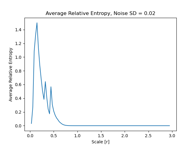
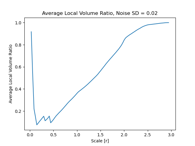
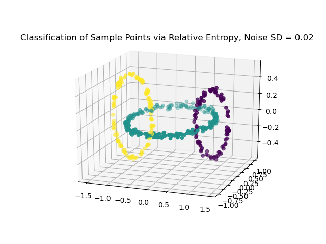
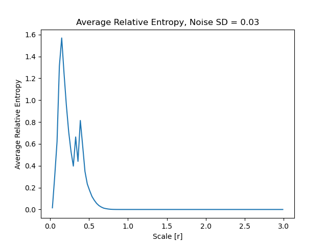
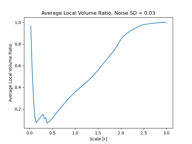
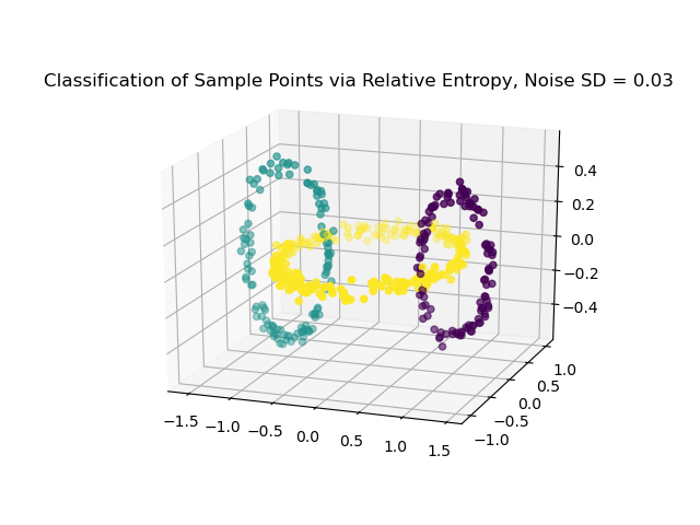
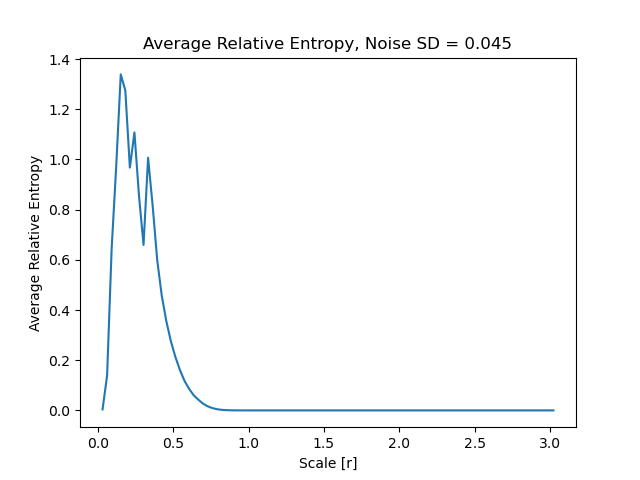
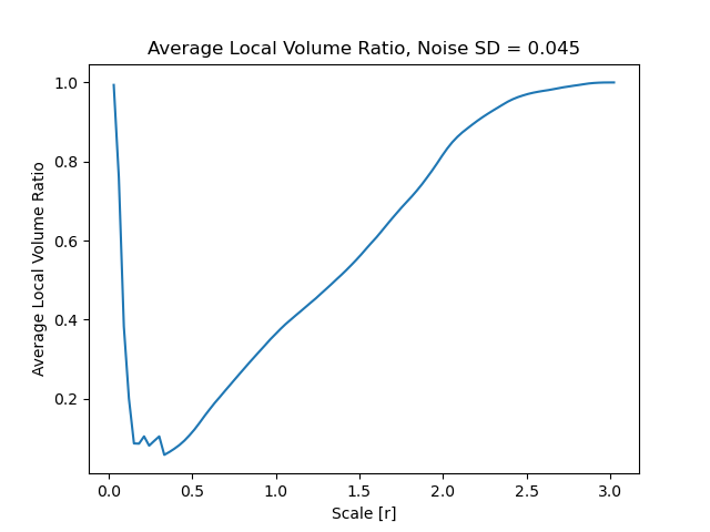
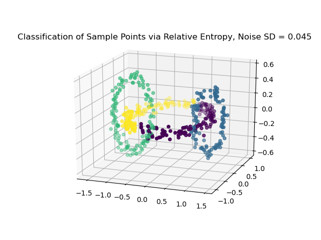
The following figures summarize the output of this algorithm on a data set of 500 points sampled with a small amount of Guassian noise from three interlinked circles embedded in $\mathbb{R}^{3}$ . The horizontal circle has radius $1$ and center $(0,0,0)$ , and the other two have radii $0.5$ and $0.4$ and centers $(0,-1,0)$ and $(0,1,0)$ , respectively. We ran several trials with different levels of Gaussian noise, with standard deviations $0.02$ (low noise), $0.03$ (medium noise), and $0.045$ (high noise). The value of $\hat{r}$ given by both methods was identical for the low noise experiment, and the algorithm correctly assigned all of the points to their respective circles. In the medium noise experiment, the Average Relative Entropy Method continues to classify the circles correctly, but the Average Neighborhood Volume Method simply puts all of the circles into a single cluster. For the high noise experiment, we see that the Average Relative Entropy Method also starts to break down, but nonetheless identifies subclusters of the circles, from which a user would be able to reconstruct the original circles. In contrast, the Average Local Volume Ratio groups all of the points into a single cluster. We therefore see that, while both methods work in ideal conditions, the Average Relative Entropy method is far more robust to noise. Interestingly, too, both the relative entropy curves and the local volume ratio curves exhibit local maxima and minima, respectively, where the smaller circles join the same group as the central circle, behavior reminiscent of the "barcodes" in topological data analysis. We include the figures below.

6.1. Low Noise Experiment ( $\sigma=0.02$ )

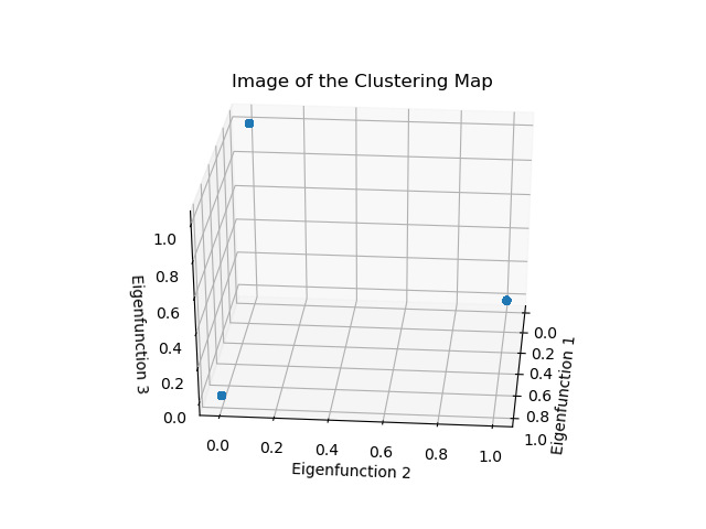
In this experiment, both methods successfully recovered the circles. Figure 6.1 illustrates the data set, Figure 6.2 shows the Average Relative Entropy at each scale, Figure 6.3 gives the plot of the Average Local Volume Ratio at each scale, Figure 6.4 shows the image of the map $\Psi$ , and, finally, Figure 6.5 shows the classification of the points. Note that in Figures 6.2 and 6.3, the joining of the two smaller circles to the group of the large circle is indicated by the second and third local maxima and minima, respectively.

Refer to caption — Figure 6.1. 500 points sampled from three circles with Gaussian noise ( $\sigma=0.02$ )

6.2. Medium Noise Experiment ( $\sigma=0.03$ )

In this experiment, the Average Relative Entropy Method successfully recovered the circles, and the Average Local Volume Ratio Method returned a single cluster of all three circles. Figure 6.6 illustrates the data set, Figure 6.7 shows the Average Relative Entropy at each scale, Figure 6.8 gives the plot of the Average Local Volume Ratio, and Figure 6.9 shows the classification of the points. The image of $\Psi$ is roughly identical to the previous experiment, so we do not repeat the plot here. Note that, in contrast to the previous experiment, the global minimum of the Average Local Volume Ratio occurs at the third local maximum.

6.3. High Noise Experiment ( $\sigma=0.045$ )

In this experiment, we see the manner in which the Average Relative Entropy Method begins to break down. While it successfully identified the two smaller circles, the large, central circle is split into two clusters. While not ideal, the circles could nonetheless be reconstructed from this clustering. As in the medium noise experiment, the Average Local Volume Ratio Method returned a single cluster of all three circles. Figure 6.10 illustrates the data set, Figure 6.11 shows the Average Relative Entropy at each scale, Figure 6.12 gives the plot of the Average Local Volume Ratio, and Figure 6.13 shows the classification of the points by color. The image of $\Psi$ is roughly identical to the previous experiment, so we do not repeat the plot. As in the medium noise experiment, the global minimum of the Average Local Volume Ratio is found at the third local minimum, i.e. after all of the circles have been joined to the same cluster.

7. Discussion and Future Work

We have presented two novel data clustering algorithms for data sampled from a uniform distribution on a disconnected metric space $X$ , possibly corrupted by Gaussian noise. Both algorithms work by identifying a scale $\hat{r}$ with which to build a graph on the points, after which they identify the connected components of the graph using the associated graph Laplacian. Unlike other commonly used clustering algorithms, this technique is completely data driven, and does not require any additional parameters. In particular, the algorithms output the number of clusters as well as the clustering, unlike the popular $k$ -means algorithm, which requires the number of clusters as input. Of the two algorithms presented, the Average Relative Entropy Method outperformed the Average Local Volume Ratio Method in terms of robustness to noise.

We remark, however, that the success of these particular algorithms, is highly dependent on the assumption of uniformity of the underlying, non-noisy distribution. This, unfortunately, prevents the current form of these algorithms from producing a correct clustering when applied to many datasets, and the adaptation of these techniques to non-uniform distributions is the subject of ongoing research. We also note that the Average Relative Entropy Method may be seen as a variation of Diffusion Maps [5] and Laplacian Eigenmaps [1], where the choice of free parameter is done in an automatic, data-driven fashion, which allows for clustering to be achieved directly from the eigenvectors of the operators, instead of after a dimension-reduction step. While our method depends on the kernel function having compact support, which is not the case in either Diffusion Maps or Laplacian Eigenmaps, and in this paper we have concentrated on the clustering problem, it would be interesting to extend the applicability of these model selection methods to dimension-reduction problems as well.

Acknowledgements

We would like to thank Robert Adler, Jacob Abernathy, and Bertrand Michel for useful discussions and comments on an earlier, preliminary version of this work. We would additionally like to thank the organizers of the CIMAT Differential Geometry Seminar, the organizers of the AUS-ICMS Meeting, the XXIst Oporto Meeting on Topology, Geometry, and Physics, and the Toposys Network for the opportunity to present our preliminary results in their conferences and seminars.

References

[1] M. Belkin and P. Niyogi (2003) Laplacian Eigenmaps for Dimensionality Reduction and Data Representation. Neural Comput. 15 (6), pp. 1373–1396. External Links: ISSN 0899-7667, Link Cited by: §1, §7.
[2] G. Carlsson (2009) Topology and data. Bull. Amer. Math. Soc. (N.S.) 46 (2), pp. 255–308. External Links: ISSN 0273-0979, Link, Review MathReviews Cited by: §1.
[3] F. Chazal, L. J. Guibas, S. Y. Oudot, and P. Skraba (2013) Persistence-based clustering in riemannian manifolds. Journal of the ACM 60 (6). Cited by: §1.
[4] F. R. K. Chung (1997) Spectral graph theory. CBMS Regional Conference Series in Mathematics, Vol. 92, Published for the Conference Board of the Mathematical Sciences, Washington, DC; by the American Mathematical Society, Providence, RI. External Links: ISBN 0-8218-0315-8, Review MathReviews Cited by: Theorem 3.2.
[5] R. R. Coifman and S. Lafon (2006) Diffusion maps. Appl. Comput. Harmon. Anal. 21 (1), pp. 5–30. External Links: ISSN 1063-5203, Link, Review MathReviews Cited by: §1, §7.
[6] D. L. Donoho and C. Grimes (2003) Hessian eigenmaps: locally linear embedding techniques for high-dimensional data. Proceedings of the National Academy of Sciences 100 (10), pp. 5591–5596. External Links: http://www.pnas.org/content/100/10/5591.full.pdf+html, Link Cited by: §1.
[7] R. Ghrist (2008) Barcodes: the persistent topology of data. Bulletin of the American Mathematical Society 45 (1), pp. 61–75. External Links: Link Cited by: §1.
[8] V. d. S. Joshua B. Tenenbaum (2000) A global geometric framework for nonlinear dimensionality reduction. Science 290, pp. 2319. Cited by: §1.
[9] J. Jost (2011) Riemannian geometry and geometric analysis. Sixth edition, Universitext, Springer, Heidelberg. External Links: ISBN 978-3-642-21297-0, Link, Review MathReviews Cited by: §2, §2.
[10] L. K. S. Sam T. Roweis (2000) Nonlinear dimensionality reduction by local linear embedding. Science 290, pp. 2323. Cited by: §1.
[11] R. Sanchez-Garcia, M. Fennelly, S. Norris, N. Wright, G. Niblo, J. Brodzki, and J. Bialek (2014) Hierarchical spectral clustering of power grids. IEEE Transactions on Power Systems, pp. 1–9. External Links: Link Cited by: §1.
[12] W. Shen, H. Wong, Q. Xiao, X. Guo, and S. Smale (2014) Introduction to the peptide binding problem of computational immunology: new results. Foundations of Computational Mathematics 14 (5), pp. 951–984 (English). External Links: ISSN 1615-3375, Link Cited by: §1.
[13] A. Zomorodian and G. Carlsson (2005) Computing persistent homology. Discrete & Computational Geometry 33 (2), pp. 249–274. External Links: Link Cited by: §1.

Abstract.