Solar Axion search with Micromegas
detectors in the CAST Experiment
with 3He as buffer gas
memoria presentada por
Juan Antonio García Pascual
para optar al grado de doctor
en Física
![[Uncaptioned image]](1506.02601v1/figures/logoUZ.png)
Laboratorio de Física Nuclear y Astropartículas
Área de Física Atómica, Molecular y Nuclear
Departamento de Física Teórica
Universidad de Zaragoza
Junio 2015
A mis padres,
a mi hermano
y a mi sobrino.
Acknowledgments
En primer lugar me gustaría agradecer a Igor G. Irastorza por ofrecerme la oportunidad de trabajar en el Grupo de Física Nuclear y de Partículas. También quiero agradecerte el apoyo incondicional que me has ofrecido durante estos años de doctorando. Por otra parte me gustaría resaltar tu calidad como científico y como persona.
Volviendo al principio de la historia, he de dar las gracias a Gloria Luzón por pensar en mi cuando se ofertó una plaza de doctorando en el grupo. También quiero remarcar la gran acogida que tuve en el grupo, primero quiero agradecer a mis "padrinos científicos" durante el doctorando Alfredo y Javi Galán por vuestra paciencia y vuestras lecciones en el laboratorio y en programación, añoro esas interminables discusiones en las que ninguno teníamos razón. También he tenido la suerte de tener una "madrina científica" Theopisti, gracias por tu apoyo durante este tiempo, he de confesar que me enteré al mes de empezar que eras griega y que no sé si sigo pronunciando mal tu nombre.
De una manera especial quiero agradecer las personas con las que he trabajado codo con codo durante estos años: a Paco por su dedicación y ayuda, a Xavi gracias por aguantarme durante esos largos periodos que pasamos en el CERN pegándonos con los detectores, a Juan por hacer el trabajo más fácil y más ameno, a Ángel por hacer posible esos montajes imposibles y tu alegría, a Diana por tu esfuerzo y simpatía y a Héctor Mirallas por tu devoción a la ciencia y tu compañerismo. Además me gustaría dar las gracias a todos las personas del grupo que han hecho más fácil mi trabajo: Héctor Gómez, Asun, Diego, Alicia, Susana, Laura, José Manuel, Gloria…, perdón si me he olvidado de alguien. También a Alfonso y Miguel Ángel, ya casi pareja de hecho, gracias por hacer tan divertidas las subidas a Canfranc y por vuestra ayuda. Tampoco quiero olvidarme de los del café, Carlos, Fredi, Fran, Ysrael, Patricia y Elena, éramos tantos y ahora somos tan poquitos, gracias por hacer más ameno el día a día. Estoy muy agradecido por haber tenido la oportunidad de formar parte de un grupo tan increíble.
Fuera del grupo de Zaragoza y del castellano, I acknowledge the support from the people that I met at the CAST experiment: Konstantin, Martyn, Jean Michel, Jaime, Julia, Idan, Biljana, Madalin and a special mention to the people with whom I shared pains and joys: Theodoros, Cenk and Iñaki, it was a pleasure working with you. I also want to thank the people from CEA for his support and for to be excellent hosts: Thomas for many interesting discussions y muy especialmente a Esther por tu apoyo y ayuda. También me gustaría expresar mi agradecimiento al personal del Laboratorio Subterráneo de Canfranc por el apoyo que nos dan siempre que subimos.
Dejando la ciencia a un lado quiero agradecer a mi familia el apoyo que me ha brindado durante estos años de doctorando, muy especialmente a mis padres. Por desgracia mi padre nos dejó en el trascurso de este doctorando y no le es posible leer esta memoria, papá donde quiera que estés, esto va por ti. Gracias mamá por tu compresión en estos difíciles años, parece que tu niño se está haciendo mayor. A mi hermano Javi quiero agradecerle todo el apoyo que me ha mostrado durante este tiempo y a mi sobrino Juan por la alegría que nos das, espero que algún día leas este documento y lo que es más difícil, que te resulte interesante. También quiero darte las gracias a ti, Ale, por el cariño que me demuestras todos los días, sin tu apoyo y comprensión estaría perdido.
Por último y no menos importante quiero agradecer a todos los amigos que he cosechado durante este tiempo por su amistad y apoyo. A los que he ido haciendo por Zaragoza: Machín mi inseparable compañero de piso y de aventuras, Mario, Carlos, Laura, Nacho, Chisco, Kosko, Manu, David,…, sois tantos que seguro que me olvido de alguien. También a la cuadrilla de Logroño: Dani, Lobo, Alex, Miguel, Fer, Jorge, Rubén, Cebo y Javo. Estoy realmente agradecido que que me llaméis amigo.
Finalmente quiero agradecer al lector que llegue más allá de esta página, espero que disfrutes con este trabajo. A pesar de haber sido redactado por un humilde servidor, encierra el trabajo, dedicación y apoyo de mucha gente.
Chapter 0 Axions and Axion Like Particles
1 Introduction
Axions are well motivated particles proposed in an extension of the Standard Model (SM) as a solution to the CP problem [1] in strong interactions. On the other hand, there is the category of axion-like particles (ALPs) which appear in diverse extensions of the SM and share the same phenomenology of the axion. Axions and ALPs are hypothetical neutral particles which interact weakly with matter, being candidates to solve the Dark Matter (DM) problem.
Several experiments have been developed for axion and ALPs detection, based on laboratory regeneration searches, galactic halo searches (haloscopes) and solar searches (helioscopes), which will be briefly discussed in this chapter. The helioscope technique, which is the main topic of this work, will be explained in detail.
2 The strong CP problem in QCD
The Quantum Chromodynamics (QCD) is a gauge field theory that describes the properties of the strong interactions between quarks and gluons, being the SU(3) component of the SM. A problem appears in QCD, the so-called strong CP problem. The theory predicts a CP-symmetry violation in strong interactions which have not been observed experimentally. The strong CP problem is closely related to the U(1)A problem of QCD and to its solution proposed by ’t Hooft in 1976, some features of this problem will be briefly described is this section.
1 The U(1)A problem and its solution
The Lagrangian of QCD can be written as:
| (1) |
where are the field strength tensors of the gluon fields with a color index a=1,…,8; are the quark fields with the quark flavor and the corresponding quark masses. is the covariant derivative defined as where is the coupling constant and are the generators of the group of rotations of the quark fields in the color space.
The QCD Lagrangian has a large global symmetry in the limit of vanishing quark masses ; U(N)V U(N)A, thus it is invariant under global axial and vector transformations. In reality and quarks masses could be considered approximately zero because , being the dynamical scale of the theory. So strong interactions are expected to be approximately U(2)V U(2)A invariant. Indeed, U(2)V = SU(2)V U(1)V is the vector symmetry corresponding to isospin times baryon number, being a good approximate symmetry in nature.
However, the corresponding axial symmetries have not been observed. This phenomenon is understood because the SU(2)A symmetry is not preserved by the QCD vacuum and by spontaneous breaking we get the Nambu-Goldstone bosons (the pions), whose mass vanishes in the limit . But there is no pseudoscalar state with vanishing mass corresponding to the Nambu-Goldstone boson of a U(1)A symmetry, this is known as the U(1)A problem [2].
The resolution of the U(1)A problem came through the realization by t’Hooft [3, 4] that the QCD vacuum has a more complicated structure. The problem was bypassed by introducing an anomalous breaking of the U(1)A symmetry, adding an extra term to the Lagrangian:
| (2) |
here is the gluon field strength tensor and its dual, the coupling constant and is an arbitrary angle between 0 and 2, which arises from the complicated structure of the QCD vacuum. More precisely, this means that the ground state is a superposition of an infinite number of degenerate states . The ground state, also called -vacuum can be expressed as:
| (3) |
Taking into account the electroweak interaction, the angle in equation 2 has to be substituted by :
| (4) |
where is the quark mass matrix, thus the Lagrangian becomes:
| (5) |
and the QCD Lagrangian can be written as:
| (6) |
This additional term in the Lagrangian solves the U(1)A problem but is not invariant under CP, which leads to the strong CP-problem.
2 The strong CP problem
For a non zero choice of in equation 5 the CP symmetry is expected to be violated as it actually occurs in electro-weak interactions, but experimentally the CP violation is not observed in strong interactions. This is the case of the electric dipole moment of the neutron (nEDM) which has been estimated by the MIT (Massachusetts Institute of Technology) bag model [5]:
| (7) |
here R is the bag radius , the quark mass ratios are estimated to be , and the bag value MeV, obtaining e cm.
Experimentally the nEDM is bounded to e cm (90 C.L.) [6], it constraints . Such small value of is allowed in the theory, however the problem is beyond the unexplained smallness of . It implies that the two contributions of equation 4, which are in principle unrelated, have to cancel each other with a precision of . The strong CP problem is why this angle coming from the strong and weak interactions, is so small.
There are mainly three solutions proposed in order to solve the CP-problem: the first and least likely implies zero quark masses, the second one is to set , imposing CP symmetry in the QCD Lagrangian and the third and more compelling solution is the Peccei-Quinn mechanism that will be described below.
3 The Peccei-Quinn solution
The Peccei-Quinn (PQ) solution was proposed in 1977 [7, 8]. In order to equal to zero it postulates a new global and chiral symmetry U(1)PQ (the PQ symmetry) that is spontaneously broken at the energy scale of the symmetry . It implies the existence of a new field which appears as the pseudo Nambu-Goldstone boson of the new symmetry, the axion. This new field yields an additional term in the QCD Lagrangian
| (8) |
where is given by
| (9) |
The first term take account of the kinetic energy, the second term represent further interactions of the axions and the third term introduces the axion field and its coupling to gluons. is a parameter dependent of the model, is the strong coupling constant and is the energy scale of the spontaneous breaking of the PQ symmetry. The third term in equation 9 provides an effective potential for the axion field , so the vacuum expectation can be obtained by calculating its minimum.
| (10) |
Thus, the value for the vacuum expectation of the axion field , can be written as:
| (11) |
It solves the strong CP problem by canceling the term for any value of , providing a dynamical solution to the problem. Expanding around its minimum the axion get mass:
| (12) |
So far the PQ mechanism is the more elegant solution to the strong CP problem and could be experimentally proven by the discovery of a new particle: the axion.
3 Axion properties.
The PQ solution fixes some properties of the axion that only depend on the energy scale of the spontaneous breaking of the symmetry . These properties are the axion mass and the coupling constant of the axion to other particles denoted by , both of them are inversely proportional to .
| (13) |
1 Axion coupling to matter
Although some of the other properties of the axions are model-dependent, generically the axion couples with gluons and photons, which is a consequence of the former. Axions could also interact with fermions. Some features of these interactions will be described below.
Coupling to gluons
The coupling of axion with gluons is given by the third term in equation 9, by the expression:
| (14) |
with the strong fine-structure constant . Due to its coupling with gluons, axions can acquire mass by mixing with pions
| (15) |
here MeV is the pion mass and MeV the pion decay constant, and are the quark masses ratios and respectively. The coupling of gluons to axion is generic to all the models, thus the axion mass mass, given by 15, is inversely proportional to .
Coupling to photons
Axion couples to photons through the mixing of pions with axions. The contribution of the axion-photon interaction to the Lagrangian is given by the expression:
| (16) |
here is the coupling constant from axions to photons, is the electromagnetic field-strength tensor and its dual, and are the electric and magnetic fields and is the axion field. A further contribution in the coupling can appear in models in which standard fermions carry PQ-charges in addition to the electric charges. The axion-photon coupling constant can be written as:
| (17) |
here is the fine structure constant, is the ratio between the electromagnetic and color anomalies, and are the quark mass ratios introduced in equation 15. Since is a model dependent factor, the terms in the parenthesis of equation 17 are usually presented in literature as the coefficient .
| (18) |
The axion-photon coupling is generic to all the models and most of axion searches strategies are based on this interaction.
Coupling to fermions
Depending on the model, axions can also couple with fermions, this interaction is postulated in the second term of the Lagrangian from equation 911 1 Note that the second term in the Lagrangian of equation 9 is defined as , in which the interaction of an axion to a fermion is given by:
| (19) |
where is the fermion field, the fermion mass and the axion-fermion coupling constant, that can be written as [9]:
| (20) |
The dimensionless combination of plays the role of a Yukawa coupling with an effective PQ-charge and a fine-structure constant of the axion can be defined.
The axion could also couple to electrons at tree level, this process is possible if electrons carry PQ-charge, thus the coefficient . This is the case of the DSFZ model (see section 2) in which the axion-electron coupling constant is given by
| (21) |
Even if the effective PQ-charge , axions could couple to electrons in a higher order. This is the so-called radiatively induced coupling at the one loop level, however the coupling is weaker than .
Finally, an effective axion-nucleon coupling could be considered since there are no free quarks below the QCD scale MeV. There are two contributions to the axion-nucleon coupling: the coupling to light quarks at tree level and the mixing with pions. The coupling constant is given by
| (22) |
here is a model-dependent coefficient of the interaction in which the coupling to protons and neutrons have different contributions.
Further processes
There are processes involving axions quite relevant in the frame of astrophysics. The predominant emission process of axion in stars is the Primakoff effect , in which a photon can be converted into an axion in the presence of strong electromagnetic fields (e.g. the electric field of the charged particles inside the plasma). This process is quite relevant in axion searches because axions could be reconverted into photons (and detected) inside a strong magnetic field via inverse Primakoff effect.
Further processes in axion models with tree-level coupling to electrons might dominate the axion emission in white dwarfs and red giants. These processes are the Compton and the Bremsstrahlung emission . Also, the axion-nucleon Bremsstrahlung could be relevant in supernova explosions.
These processes and its implications in astrophysics will be revisited in section 3
2 Axion models
Axion could couple to different particles as it was presented in the previous section. These interactions are strongly model dependent and can be divided in two different trends: the first postulated axion also referred to visible or PQWW (Peccei-Quinn-Weinberg-Wilczek) axion and the invisible axion model which assumes a lighter axion.
Visible axion model
In the original PQ model [10], the symmetry was broken at the electroweak scale with GeV. It implies axion masses larger than keV and relative strong coupled to baryonic matter and radiation. Such axions would have been produced and detected in reactor and accelerator experiments. The non experimental observation of the PQWW axion together with the astrophysical limits on the evolution of the red giants ruled out the existence of the visible axion.
Invisible axion models
After the dismiss of the visible axion, a new invisible axion model was postulated. Indeed, the breaking scale of the PQ symmetry is an arbitrary value that could be larger than the electroweak scale. There are mainly two different invisible axion models, the KSVZ (Kim-Shifman-Vainshtein-Zakharov) and the DFSZ (Dine-Fischles-Srednicki-Zhitnitskii), in both of them the axion is light and interact weakly with matter.
KSVZ model
In this model [11, 12] the interactions of axions with matter only occurs via the axion-gluon coupling and ordinary quarks and fermions do not interact with axions. A new heavy quark has to be introduced, being the unique particle which carries PQ charge in the KSVZ model. However, the axion would still interact with the light quarks due to the color anomaly. The axion-photon coupling is given by equation 17 in which is a model dependent parameter, in general in the KSVZ model is given by:
| (23) |
where is the electric charge of the new heavy quark and can take values of . The most common values used in the literature are , and the standard KSVZ model with , that are shown in figure 1.
DFSZ model
In contrast with the KSVZ model, in the DSFZ model [13] the fundamental fermions carry PQ charge and no exotic quark is needed. The disadvantage of this model is that a fine tuning is necessary in order to obtain a breaking scale larger than the electroweak scale. On the other hand, the advantage of this model is that it can be easily introduced in Grand Unification Theories (GUT). In this case the model dependent parameter takes the value (see figure 1).
3 Summary of relevant axion constraints
The axion mass is initially arbitrary since the strong CP problem is solved for any value of the breaking scale . Due to its implications in astrophysics, cosmology and particle physics, the axion has been thoroughly studied and the most relevant constraints come from astrophysical considerations. Indeed, axions could be produced in hot and dense environments like stars, globular clusters and white dwarfs.
Solar model
Axions could be produced in the solar plasma via Primakoff effect and electron Bremsstrahlung processes, being an additional energy loss channel that could reduce the lifetime of the star. The most relevant constraint comes from the fact that the emission of axions from the Sun implies an increment of the nuclear burning and consequently, of the solar temperature distribution, that leads an increase in the 8B neutrino flux [15]. With these considerations the axion-photon coupling is constrained to GeV-1. Also, the axion-electron coupling is constrained to GeV-1 by the Bremsstrahlung collisions.
Globular clusters
A globular cluster is a spherical collection of of densely packed stars that were formed about the same time. Two different types of stars in globular clusters are especially interesting for the axion bounds, the horizontal branch (HB) stars and the red giant branch (RGB). The RGB stars have degenerated helium burning core and a hydrogen burning shell. When the RGB helium core becomes hot and dense enough it rapidly increases the rate of fusion and becomes a HB star. Thus the axion production via Primakoff effect should be larger in HB stars in comparison with RGBs, adding a new energy loss channel which is negligible for RGB stars. So the population of RGB stars should be relatively larger than the population of HB stars inside the globular clusters. By computing the observed population of HB and RGB stars [9], the axion-photon coupling is constrained to GeV-1, being the most restrictive astrophysical limit on the coupling constant.
Also the RGB stars are supposed to have larger brightness if the degenerate helium core losses too much energy by emission of axions or neutrinos. In this case the axion emission would be dominated by electron-Bremsstrahlung processes. Observational measurements in the globular cluster M5 [16] lead to a limit on the axion-electron coupling of GeV-1.
White dwarf cooling
White dwarfs (WD) are a remnant of initial low massive stars, made of a degenerate carbon-oxygen core and a helium burning shell. A WD is very hot when it is formed, but since it has no energy source it gradually cools down, by first the emission of neutrinos and later by photons from the surface. Also, WD could increase its cooling speed by the emission of axions generated mainly by axion-Bremsstrahlung processes. This axion emission could be constrained by the comparison of the observed cooling speed with WD models. One special case is the study of the cooling of the ZZ Ceti stars [17] in which the most restrictive limit on the axion-electron coupling GeV-1 has been obtained.
Supernova 1987 A
A supernova (SN) is a stellar explosion that expels a big quantity of stellar material with a great force. There are different types of SN, the most interesting one is the type II SN. When a star is massive enough to burning its carbon-oxygen core (in contrast with white dwarfs), it rapidly consumes the carbon core producing heavier nuclei and increasing the core size, at some point the core exceeds the Chandrasekhar limit22 2 The Chandrasekhar limit is the maximum mass that can be supported by electron degeneracy pressure without suffering a gravitational collapse [18] and the star collapses. A cataclysmic implosion takes place within seconds generating a huge quantity of radiation and a burst of neutrinos.

Axions could be emitted from the core of a type-II SN via axion-nucleon Bremsstrahlung shortening the neutrino burst. For a very small axion-nucleon coupling , the duration of the burst is not affected, but by increasing the coupling, the burst duration becomes shorter until it reaches its minimum (free streaming regime in figure 2). Also, if increases further, axions are not able to escape (trapped regime in figure 2) and the burst duration becomes unaffected.
The SN 1987A gave the first chance to observe directly the neutrino emission from an extragalactic source, it was measured by the neutrino experiments IMB33 3 Irvine-Michigan-Brookhaven detector and Kamiokande II44 4 Kamioka Nucleon Decay Experiment operating at this time. A total of 20 neutrinos were detected with a burst duration of s which fits the expectations without an extra axion cooling. These measurements lead to an excluded range on the axion-nucleon coupling of [19]. However, the low statistics accumulated from the neutrino burst and some incompatibilities in the measurements of the two different experiments create a big uncertainty in this excluded range.
4 Axions as a Dark Matter candidate
There are several observational evidences of the presence of Dark Matter (DM) in the Universe, like the rotation curves of the spiral galaxies, gravitational lensing and fluctuations in the Cosmic Microwave Background (CMB). According with the latest results of the PLANCK experiment [20] the Universe is composed of a 4.2% of baryonic matter, a 27.2% of DM and a 68.6% of Dark Energy (DE); in other words, the most part of the Universe has an unknown nature. The DE takes account of the accelerated expansion of the Universe, but his nature is not well understood, it can be explained as a cosmological constant, vacuum energy or a quintessence field.
The DM would be composed by electrically neutral particles which interact weakly with matter. Popular candidates to DM are the Weakly Interacting Massive Particles (WIMPs) which appear in supersymmetry models and are searched in several underground experiments. The axion is also an attractive DM candidate, axions could be thermally produced in the primordial plasma, but being light particles, they would contribute to the hot DM as neutrinos do. This production mechanism is more efficient for larger masses, so cosmological observations constrain the amount of hot DM and fix an upper bound in the axion mass of eV [14]. Other two related mechanisms could have produced non-relativistic axions in an early Universe: the vacuum realignment and the decay of the topological defects which make the axion an attractive cold DM candidate.
In the early Universe when the temperature dropped below the PQ breaking scale , the axion field appeared with random initial conditions. This means that the initial values of the axion field were different in causally disconnected regions. Later on, during the QCD phase transition the axion potential rises and the axion acquire mass, then the axion field oscillates towards its minimum solving the CP problem dynamically. These oscillations take account of the non-relativistic axions, this is the so-called vacuum realignment [21] mechanism in which the population of the axions depends on the unknown initial value of the field. Moreover, discrete domains with topological defects like strings and walls quickly decay producing a large amount of cold DM axions. This is the decay of topological defects [22] mechanism. The great uncertainly of the axion density depends on whether the inflation happens after or before the PQ symmetry breaking.
In the case that inflation happens after the PQ symmetry breaking, the axion field is homogenized by inflation. In this scenario the topological defects are dissipated and only the vacuum realignment contributes to the cold DM axion density. Contrary to the thermal production, this mechanism is more efficient for smaller axion masses. Since the population of the axions depends on the unknown initial value of the field, by tuning the initial value of the field, there is a wide range of axions masses which gives the proper density of CDM, this is the so-called anthropic window.
If the inflation occurs before the PQ symmetry breaking, the initial conditions of the axion field are randomly distributed in causally disconnected regions and an estimation of the vacuum realignment production can be done. In this scenario the contribution of the decay of the topological defects has to be taken into account, but its calculations are not clear, it could be of the same order of the contribution of the vacuum realignment or considerably larger.
In summary, the preferred mass range for axion cold DM is eV, also referred as classic axion window [22]. Smaller axion masses are still possible in fine-tuned models and also axions with masses above the classic window can be a subdominant component of cold DM and could coexist with other exotic particles like WIMPs. Moreover, axion like particles in a wide range of space can solve the DM problem. A summary of the astrophysical and cosmological constrains on the Peccei-Quinn axion in combination with experimental searches are shown in figure 3.
4 Axion like particles (ALPs)
Although axions are the best motivated particles, there is also the category of Axion Like Particles (ALPs) or more generically Weakly Interacting Slim Particles (WISPs). ALPs share the same phenomenology of the axion, being light particles that weakly couples to two photons. The interaction can be written as:
| (24) |
where represents the ALP field and its coupling constant. In contrast with the PQ axion, ALPs are not motivated by the strong CP problem and and are independent parameters. ALPs may arise as pseudo Nambu-Goldstone bosons from extensions of the SM in which a new symmetry is broken at a high energy scale. ALPs also appear in string theory as the axion does. ALPs have an important role in the context of the low energy frontier of particle physics [23].
Beyond ALPs, in the category of WISP, there are some particles like hidden photons. They appear in extensions of the SM in which hidden sectors are included, these sectors do not directly interact via the gauge boson forces of the SM, being the interaction through the interchange of very heavy particles. Hidden photons can oscillate with standard photons via a kinetic mixing and thus they show the same behavior of the axions and its coupling with photons, in this case a magnetic field is not necessary for the conversion.
ALPs and hidden photons separately could provide all the amount of DM. The non thermal mechanisms of production are the vacuum realignment and the decay of the topological defects, the same mechanisms described for the axion, introduced in section 4. The contribution of the WISP to the total amount of DM has been recently studied [24] and a wide range of the parameter space () can contain models with the right density of DM.
5 Astrophysical hints for axions and ALPs
Several astrophysical and astronomical observations could be interpreted as hints of axions and ALPs. Like the excessive transparency of the Universe to very high energy photons (VHE) and the anomalous cooling rate of white dwarfs (WD). These hints will be briefly described below.
1 VHE transparency
Very high energy photons (VHE) with energies of TeV traveling through the intergalactic medium have a non negligible probability to interact with the background photons permeating the Universe. VHEs could interact with the extragalactic background light (EBL) via pair production . Thus, the Universe is expected to be relatively opaque to distant VHE sources like active galactic nuclei (AGN).
The EBL density is estimated by the measurements of the spectra from distant blazars by HESS [25] and Fermi [26], in good agreement with theoretical models. However, there are different observations that indicate a high transparency of the Universe to VHE photons, even in the most favored EBL models. Actually, experiments based on atmospheric Cherenkov telescopes like HESS [27] and MAGIC [28] have measured VHE photons with arrival directions clearly correlated with AGNs with an spectra which requires a low EBL density or an anomalous spectra in the origin.
The high transparency of the Universe to the VHE photons could be explained by ALP-photon oscillations. VHE could be transformed into ALPs in the local magnetic fields at the origin, in the intergalactic magnetic fields and in the Milky Way. These ALPs could travel through the intergalactic medium without interacting. These oscillations lead to a more transparent Universe to the VHE photons. This kind of ALPs [29] requires a low mass eV in order to preserve the coherence over large magnetic fields and relative large coupling constants GeV-1. Although these parameters are far away from standard axion models, ALP models in which and are uncorrelated could take account of these oscillations.
2 The WD cooling
The WD cooling was introduced in section 3 and a limit on the axion-electron coupling could be extracted from the study of the WD evolution. However, recent studies indicate an anomalous cooling speed which could be a hint of an axion emission. Indeed, the luminosity function55 5 Number of stars per luminosity interval of the WDs is predicted with a great accuracy by theoretical models. An axion emission could be a source of extra cooling and may suppress the luminosity function of the WDs at some point.
Recent works based on well studied WD models and the measurements of different WDs luminosity population point to the possibility that a small amount of energy loss coming from axions is feasible. Axions with coupling constants of [30] seem to fit the experimental measurements. Also the evolution of the pulsating period of certain WDs can provide a direct measurement of their cooling. The different pulsing of ZZ Ceti WDs, G117-B15A [31] and R548 [32] have been computed, obtaining a similar result of . These results create some tension with another limits coming from astrophysical considerations. In any case, the WD models seem to improve by adding an extra cooling coming from axions with masses above meV and can be interpreted as a hint of axions. Also, ALPs models could fit to the observed cooling rate of WDs.
6 Axion and ALPs searches
As it was presented in previous sections, axions and ALPs could be generated in an early Universe and also can be produced in hot and dense environments like stars. So that the different search strategies can be divided depending on the source: haloscopes and telescopes are looking for cold DM axions permeating the galactic halo, helioscopes that are searching Solar axions and photon regeneration experiments in which axions could be produced and detected in the laboratory. All these strategies are based on the Primakoff effect, in which axions could be converted into photons in strong electromagnetic fields. The most sensitive experiments for axions and ALPs searches are shown in figure 4. Also, the most relevant constrains and hints are drawn.

1 Galactic halo searches
Galactic halo searches could be divided in two different kind of experiments: haloscopes which are based on resonant cavities in a magnetic field and telescopes that are looking for the decay of the axion to two photons.
Haloscopes
The haloscope technique was proposed by Sikivie [33] in 1983. As it was described in section 4, axions are attractive cold DM candidates. These relic axions could be detected by resonant cavities inside strong magnetic fields, this is the so-called haloscope technique. Relic axions could be converted into photons via Primakoff effect in a magnetic field. Being these axions non relativistic, the converted photons would be monochromatic with energy around . The resonant process in the cavity is enhanced when its frequency matches . This technique only allows to scan a narrow range in the axion mass. However, the resonant cavity is tunable and the data taking could be performed by scanning narrow ranges of .


The first haloscopes were developed by Rochester-Brookhaven-Fermilab (RBF) and the University of Florida (UF) [35]. They demonstrate the technique in a wide range of axion masses eV but with a poor sensitivity (see figure 5 top). Later on, a second generation haloscope was developed, the Axion Dark Matter eXperiment (ADMX), being the first haloscope with enough sensitivity to reach the most favored axion models. In a first stage ADMX scanned an axion mass region from eV [36], in a second phase the microwave receivers was substituted by SQUID (Superconducting QUantum Interference Device) in order to improve the sensitivity and scanning a mass range from eV [37] (see figure 5 bottom). However, these results assume that axions are the main component of cold DM in the Universe.
Telescopes
Although the decay of the cold DM axions to two-photons is expected to be extremely odd, it could be detected in thermally produced axions in the eV regime. The signal will be a closely monochromatic line emitted from galaxies and could be observed by telescopes used in astrophysics. Different works have excluded axion masses of eV [38, 39].
2 Laboratory searches
In laboratory experiments, photons could be converted into axions or ALPs inside a strong magnetic field via Primakoff effect. The advantage of this technique is that it does not rely in astrophysical or cosmological assumptions about the origin of the axions or ALPs. On the other hand, the sensitivity of this kind of experiments is usually lower than other search strategies. There are mainly two different techniques in laboratory searches: the Light Shining through Wall (LSW) and the polarization experiments.
LSW searches
LSW or photon regeneration experiments [40] use high intensity laser beams inside a strong transverse magnetic field in order to produce axions or ALPS, in which an opaque wall is placed to block the photons. On the other side of the wall another magnetic field allows the axions or ALPs, which could easily pass the wall, to be transformed again into photons that can be detected.
Several experiments have excluded significant regions in the ALP parameter space: the LIPSS66 6 LIght Pseudoscalar or Scalar Search[41] experiment at the Jefferson Laboratory, the BMV77 7 Birefringence Magnetic du Vide[42] collaboration, the GammeV88 8 Gamma to mili-eV particle search[43] experiment at Fermilab, the OSQAR99 9 Optical Search for QED vacuum magnetic birefringence[44] experiment working at CERN and finally the most sensitive LSW so far, the ALPS1010 10 Axion-Like Particle Search[45] experiment at DESY. The results of all these experiments are shown in figure 6. Although the experiments related before use laser beams, the same principle of detection could be adapted to the microwave regime. This is the case of the CROWS1111 11 CERN Resonant Weakly Interacting sub-eV Particle Search experiment [46] at CERN.

Polarization experiments
In contrast to LSW experiments, it is possible to obtain an axion signal in the laser beam itself. When a polarized light passes through a transverse magnetic field it could generate axions or ALPs and thus, it would induce a detectable small rotation and ellipticity in the laser beam.
Experiments like the BFRT1212 12 Brookhaven Fermilab Rutherford Trieste collaboration[47] at the Brookhaven National Laboratory and the PVLAS1313 13 Polarizzazione del Vuoto con LASer experiment at the the Legnaro National Laboratory exploited this technique and excluded some regions of the parameter space (see figure 6). Moreover, the PVLAS experiment reported a signal, but it was ruled out later on since it was interpreted as an artifact of an instrument [49].
3 Solar axion searches
The Sun is expected to be a powerful axion source as it was presented in section 3. Solar axions could be detected in the laboratory via inverse Primakoff effect. Two different techniques for the detection of solar axions have been developed: helioscopes and Bragg scattering experiments.
Helioscopes
The helioscope technique was proposed by Sikivie [33] in 1983. The principle of detection is to reconvert the solar axions into photons inside an intense transversal magnetic field. Solar axions may have energies in the keV regime, thus the expected signal are X-rays in the detectors located at the edges of the magnet. Helioscopes can cover axion masses in a wide range of the parameter space (up to eV) because contrary to haloscopes, the signal is independent of the axion mass. The helioscope technique will be revisited in more detail in section 7
Different experiments based on the helioscope technique have been developed, the first one was performed by Lazarus et al. [50] validating the technique. Later on, the Tokyo Axion Helioscope (SUMICO) [51] applied the same principle of detection increasing the sensitivity. Finally, the CERN Axion Solar Telescope (CAST) started in 2003 being the most sensitive helioscope until now. The excluded regions of these experiments together with the Bragg scattering searches are shown in figure 7.
The CAST experiment, which is the main topic of this work, will be detailed in chapter 1.
Bragg scattering searches
Crystalline detectors can also be used for solar axion searches. The axion-photon conversion could take place in the Coulomb field of the nuclei in the crystal lattice. The conversion occurs when the angle of the incident axions fulfills the Bragg condition with the plane of the crystal. Thus, the expected signal is a characteristic Bragg pattern in the detector.
Even though there are not many dedicated experiments, a great number of underground experiments developed for WIMP searches have been looking for these patterns. Such as SOLAX1414 14 SOLar AXion search in Argentina[52], COSME1515 15 Germanium detector located in the Canfranc Underground Laboratory[53], DAMA1616 16 DArk MAtter searches, operating at Gran Sasso[54], CDMS1717 17 Cryogenic Dark Matter Search, located in Soudan[55] and more recently EDELWEISS1818 18 Expèrience pour DEtecter Les Wimps En Site Souterrain, at Modane[56]. However, the sensitivity of this technique cannot compete with dedicated helioscope experiments, as is shown in figure 7.
7 Solar axions and the helioscope technique
Axions could be generated in the core of the Sun, being the most powerful axion source closest to the Earth. The expected production of axions in the well known Solar Model will be described in the next section. The detection of solar axions comes through its conversion into photons inside strong magnetic fields in which the probability of the axion-photon conversion has an important role and will be further detailed.
1 The Solar Model and the axion production
The solar axion flux can be extracted from the well established Standard Solar Model. The most relevant channel in the axion emission comes from the Primakoff conversion which is dominant in hadronic axion models such as the KSVZ model. In the case of non-hadronic axions (DFSZ model) with a tree level interaction with electrons, other processes have to be taken into account: Bremsstrahlung, Compton and axion recombination. The contribution of these channels could be considerably larger than the Primakoff emission. However, in the helioscope technique only the Primakoff contribution is usually taken into account because it is more reliable to suppose the same processes involving the generation and detection of the axions. Also the astrophysical constraints on are more restrictive than the limits that in principle could be reached with helioscopes.
Hadronic axion emission
Axions could be generated in the core of the Sun inside the strong electric fields from the charged particles of the solar plasma by the process . Thus, the energies of the converted axions correspond to the blackbody radiation of the core of the Sun (keV regime).
The Primakoff process in non-relativistic conditions is relevant when the mass of electrons and nuclei are larger than the energies of the ambient photons. Following [9], neglecting recoil effects, the differential cross section is given by:
| (25) |
here is the charge () of the involved particle, is the fine structure constant, and are the momentum of the photon and the axion respectively and is the momentum transferred.
The cut-off of the Coulomb interaction in vacuum for is given by the minimum momentum transfer for and the total cross section can be written as:
| (26) |
In a plasma, the Coulomb potential is cut-off due to screening effects and thus the differential cross section is modified by an additional factor in equation 25.
| (27) |
In a non degenerate medium, the screening scale is given by the Debye-Hückel formula
| (28) |
where is the temperature of the solar plasma, is the baryon density and and are respectively the fraction of electrons and different nuclear species per baryon. Using equations 27 and 28, the total scattering cross section can be calculated. Summing over all the targets, the transition rate of a photon with energy into an axion of the same energy is obtained.
| (29) |
here, the effective photon mass and axion mass are negligible in comparison with . The differential axion flux at Earth can be calculated by the convolution of the transition rate and the blackbody emission of the Sun.
| (30) |
being km the average distance from Earth to Sun and km the solar radius. Using the Standard Solar Model from [57] an analytical approximation of the axion differential spectrum can be derived [59].
| (31) |
The differential solar axion flux is proportional to the coupling constant with an average energy of keV and a maximum around 3 keV (see figure 8). Also the total axion luminosity of the Sun has been estimated:
| (32) |
where is the solar luminosity.
Non-hadronic axion emission
In non hadronic axion models with an axion-electron coupling at tree level (DFSZ model), the solar axion emission is dominated by the axion-electron coupling. Following the work of Redondo [60], the most important production comes from the interactions: electron-ion Bremsstrahlung , electron-electron Bremsstrahlung , Compton scattering , axio-recombination and axio-deexcitation . The Feynman diagram of these processes together with the Primakoff process are shown in figure 9.

The Bremsstrahlung or free-free (ff) electron transitions on hydrogen and helium nuclei dominates solar flux together with the electron-electron (ee) Bremsstrahlung. The axio-recombination, also know as free-bound (fb) electron transitions, of metals (mainly O, Ne, Si, S and Fe) has a significant contribution. The axio-deexcitation, or bound-bound (bb) electron transitions, is dominated by Lyman transitions (mostly Ly-) being significant in the case of iron ( keV). The Compton (C) production process has a poor contribution.
The emission rate of solar axions for all the processes described before, can be expressed as:
| (33) |
where is the emission rate of the sum over all the processes.
Electron-ion Bremsstrahlung, axio-recombination and axio-deexcitation
In processes in which a photon is emitted when a electron makes an atomic transition . The spin-averaged matrix element of emitting an axion of energy is proportional to the analogous matrix element of emitting a photon of the same energy. Thus in this case the emission rates of photons and axions are proportional and can be formulated as:
| (34) |
In the case of the electron-ion Bremsstrahlung (ff), the photon production rate is given by:
| (35) |
where is the charge of the involved nuclei and its number density, is the electron density, take account of the screening effects and is the screening scale introduced in equation 28. Therefore the transition rate for electron-Bremsstrahlung processes can be derived:
| (36) |
Electron-electron Bremsstrahlung
In this case the expression 34 is not valid because the photon emission is highly suppressed in comparison with electron-ion processes. The production rate involving this process has been calculated in [9] and is given by:
| (37) |
Compton scattering
In the non-relativistic limit, the cross section of the axion production in Compton-like processes is given by [19]:
| (38) |
Thus the transition rate can be expressed as:
| (39) |
here the ratio between the photon and the axion production rate is slightly different from equation 34.
| (40) |
All the contributions to the axion emission presented before can be expressed in terms of the photon absorption coefficient with the exception of the electron-electron Bremsstrahlung. Thus, the total axion flux in earth can be calculated analogous to equation 30
| (41) |
where is the emission rate of all the processes presented in 33, this term depends on the local parameters of the solar plasma. By integrating equation 41 using the solar model from [61] and the different contributions presented before, the axion flux at Earth has been extracted [60] and is shown in figure 10.

Contrary to the hadronic axion emission, the total axion flux cannot be approximated to an analytical formula, due to the narrow lines from the bound-bound and free-bound transitions. Also, the maximum of the spectrum is reached at lower energies (1 keV), in contrast with the Primakoff emission. On the other hand, the Bremsstrahlung (B) and Compton (C) processes could be approximated to an analytical formula:
| (42) |
| (43) |
here, the Bremsstrahlung flux includes electron-ion and electron-electron processes.
2 Probability of the axion-photon conversion
In the helioscope technique, solar axions could be converted into photons inside strong magnetic fields by the inverse Primakoff effect. This conversion is only effective when the magnetic field is transversal to the direction of propagation of the incoming axion. The wave equation of a particle propagating along the z-axis in a transverse magnetic field is given in [62] and can be formulated as:
| (44) |
here is the amplitude of the photon field parallel to the magnetic field, is the amplitude of the axion field, is the inverse absorption length for the photons and is the effective photon mass, which is given by the plasma frequency of the medium. A first-order solution using a perturbative approach has been derived in [59] and is given by the expression:
| (45) |
In general , and are functions of . By considering the case in which the magnetic field and the density are uniform and and are constant. The conversion probability of an axion into a photon inside a magnetic field with an effective length , can be derived:
| (46) |
where is the momentum transfer between the axions and the photons in the medium, which is given by:
| (47) |
Two different cases will be detailed below, the first one considering the conversion inside vacuum and a second case with a buffer gas inside the conversion volume.
Probability of conversion in vacuum
For the vacuum case, the probability of conversion can be simplified considering the absorption term negligible (). Applying this condition to equation 46, the probability of conversion is reduced to1919 19 Note that the relation has been applied:
| (48) |
Also in this case the effective photon mass could be considered negligible . Thus, the momentum transfer from equation 47 can be simplified.
| (49) |
This yields a condition in which the coherence is maximized for due to the sinusoidal term, that can be expressed in terms of axion mass:
| (50) |
Assuming a magnetic field of 9 T with an effective length about 10 m and an axion energy of keV, the coherence condition is fulfilled for axion masses of eV (see figure 11 top). Also, in the case of full coherence , the equation 48 can be simplified2020 20 By using the approach .
| (51) |

Probability of conversion in a buffer gas
In order to be sensitive to higher axion masses the conversion region can be filled with a buffer gas. In this case the effective photon mass from equation 47 has to be taken into account.
While in vacuum the photons are massless, an effective mass can be considered when the photons go through a medium in which the traveling speed is less than the speed of light . This can be interpreted as an effect of mixing between the photon and the quantum excitations of the matter. The effective photon mass is given by the plasma frequency of the medium :
| (52) |
here is the electron density of the buffer gas, which is related with the gas density by the expression:
| (53) |
and are the corresponding atomic number and atomic weight of the gas, the Avogadro’s number and the gas density.
The coherence is restored when the momentum transfer tends to zero (see equations 46 47), when the axion mass and the effective photon mass are equal (see figure 11 bottom). Also, the absorption could not be considered negligible and has to be taken into account. This technique has been used in helioscopes in order to scan higher axion masses by increasing the buffer gas density in small steps.
Chapter 1 The CAST experiment
1 Introduction
The CERN Axion Solar Telescope (CAST) experiment is located at building SR8 at CERN and is looking for solar axions since 2003. CAST exploits the helioscope technique using a decommissioned LHC11 1 Large Hadron Collider dipole magnet [63] (see figure 1) that provides a magnetic field up to 9 T in which solar axions could be converted into photons. The magnet is mounted on a movable platform that allows tracking the Sun 1.5 hours two times per day, during sunset and sunrise. The magnet is composed by two magnetic bores with X-rays detectors placed at the bore ends. The signal of axions would be an excess of counts in the X-rays detectors while the magnet is pointing the Sun.

The CAST research program can be divided in two phases, the first one with vacuum inside the magnetic bores and a second phase with buffer gas in which 4He and 3He were used separately in different periods. During Phase I, the X-ray detectors installed were a conventional Time Projection Chamber (TPC), a Micromegas (MICRO MEsh GAseous Structure) detector and a Charge Coupled Device (CCD) in the focal plane of an X-ray focusing device. During Phase II, the TPC was replaced by two Micromegas detectors. This chapter describes the main features of the CAST experiment together with a review of the X-ray detectors that have been working at CAST.
2 Technical description
The CAST experiment is composed by several additional systems required for the data taking operation. The magnet operates at a nominal temperature of K and a cryogenic cooling system is required. Also, a vacuum system is installed around the magnet bores in order to increase the transparency of the X-rays from the axion-photon conversion and to isolate the magnet from the environment.

The magnet is mounted on a movable platform that allows a vertical movement of and in horizontal (see figure 2). The movement of the magnet is controlled by a tracking system program which allows to point the Sun automatically. Moreover, a gas system has been installed to fill the magnet bores with a buffer gas (4He and 3He) in small steps in order to restore the sensitivity to higher axion masses. The monitoring of all the systems is performed by the slow control. The different systems of the CAST experiment will be detailed below.
1 The CAST magnet and cryogenics
The CAST magnet is one of the first prototypes designed for the LHC [64] (see figure 3). In contrast to the final bend design of the LHC, the CAST magnet has two straight beam pipes of 9.26 m that allow to exploit the total bore aperture of 4.30 cm of diameter (14.52 cm2 cross-section). The magnet is made of a superconducting Niobium-Titanium (NbTi) alloy working at a nominal temperature of K. During normal operation the magnet is loaded at 13 kA, providing a magnetic field of 8.8 T. The magnetic field is perpendicular to the beam pipes as it is shown in figure 4, which allows the axion to photon conversion in the direction of the beam pipes.

The cryogenic system is supplied with liquid helium [65], using the cryogenics from the former LEP22 2 Large Electron Positron collider and its experiment DELPHI33 3 DEtector with Lepton, Photon and Hadron Identification. The magnet is supplied by the Magnet Feed Box (MFB) placed on the top of the magnet, above the rotary pivot (see figure 2). The MFB provides liquid helium and high current to the magnet via flexible cables. The cooling of the magnet is performed in different phases, in the final stage the liquid helium becomes superfluid and circulates in a cycle over the magnet from the MFB to the Magnet Return Box (MRB).

During magnet operation an abnormal termination can occur, a part of the superconducting coils can enter in a resistive state and raise the temperature of the surrounding region. This phenomenon is called quench and can be destructive for the magnet. In order to prevent a it, a quench protection system has been installed at CAST. When the protection system is triggered, the quench heaters are activated, generating a controlled increase of the magnet temperature that is uniformly distributed. The rise of the temperature provokes an overpressure in the system and the helium is purged in order to prevent damages in the magnet.
2 The tracking system
The tracking system is crucial for the required precision of CAST while is pointing the Sun. For this purpose, an accurate hardware and software were designed [66]. Also, two complementary alignment tests are performed regularly, the grid measurements and the Sun filming. All these features will be described below.
Hardware
The CAST magnet is mounted on a movable platform that allows a vertical movement of (polar angle) and from to in horizontal (azimuth angle). The rotary pivot is placed underneath the MFB in order to ensure the stability of the cryogenics while the magnet is moving. The MRB side of the magnet is supported by a trolley with four wheels mounted on rails, which allows the horizontal movement (see figure 2). The vertical movement is performed by two jacks spinning around two lifting screws mounted on the trolley.
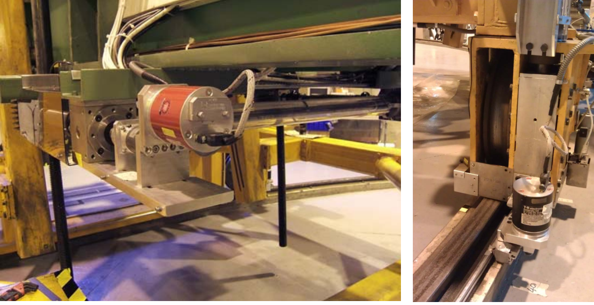
The horizontal motion is performed by a driving wheel connected to a motor, for the vertical movement another motor control the speed of the lifting jacks. Both horizontal and vertical motions are monitored by two different motor encoders (see figure 5). The values of the encoders can be translated into polar and azimuthal angles to check the orientation of the magnet.
Software
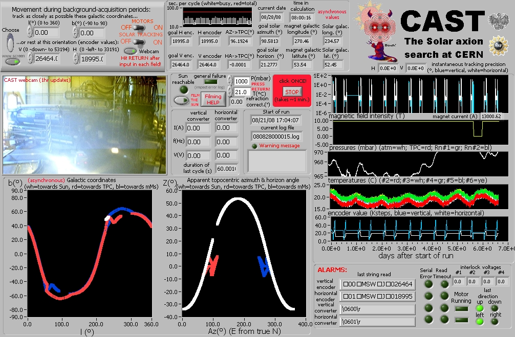
In order to perform the Solar tracking a Labview based software was developed (see figure 6). The program calculates the position of the Sun using the NOVAS44 4 Naval Observatory Vector Astrometry Software[67] software. During the tracking the program communicates with the hardware. It calculates the position of the Sun in the next minute, then the motor velocities are modified using the position of the magnet from the motor encoders. The expected and the real tracking position are monitored and thus the precision of the tracking is checked every minute.
Tracking system alignment
The precision of the solar tracking is essential in the helioscope technique. Two different methods are used in order to check the reference position of the magnet and the real one: the grid measurements and the Sun filming.

The Sun filming consists in monitoring the visible light of the Sun through a window in the experimental area. These measurements only can be performed in March and September, when the Sun is reachable. For this purpose a photo camera is aligned with the magnet and takes photos of the Sun during morning trackings. Afterwards, a software is used to compare the deviation of the center of the Sun using the reference position of the camera.
The grid measurements are performed at least once every year and consist in measuring different reference positions of the magnet that are compared with previous years. In case of any deviation of the reference position the new grid can be implemented in the software program.
3 The vacuum system
The vacuum system at CAST can be divided in different subsystems depending on its purpose (see figure 8). The cryostat vacuum isolates the magnet from the environmental temperature and the general vacuum line separates the magnet from the detectors. At the end of the line four gate valves are installed (VT1, VT2, VT3 and VT4), one per detector bore end. During normal operation the gate valves are open, but they can be closed separately in case of failure. Finally, in the detector side of the gate valves there are several vacuum subsystems for the different detector lines.

4 The gas system
The sensitivity to higher axion masses can be restored by the addition of a buffer gas inside the magnet bores. The CAST experiment has used 4He and 3He as buffer gases in different periods. In order to scan a wide range of axion masses in small steps, precise amounts of gas has to be inserted inside the cold bores and thus, an accurate gas filling system was installed.
The buffer gas has to be confined inside the magnetic field region, for this purpose four cold windows were installed at the end of the magnet bores (see figure 8). The requirements of the cold windows are: high X-ray transmission, a low leak rate of helium from the cold bore to the vacuum side and robustness against rapid increases of the pressure (e.g. during a quench).

The cold windows are made of 14 m polypropylene foil glued on a stainless steel grid structure also called strongback (see figure 9). The cold windows was manufactured and tested by the CERN Central Cryogenics Laboratory (Cryolab).
The gas system was upgraded when the 4He was replaced by 3He. Since the 3He is an extremely expensive gas, additional systems were installed to prevent any leak [68]. A scheme of the filling system is shown in figure 10 in which the different elements are labeled: storage volume, purging system, metering volumes and expansion volume.

The storage volume has a capacity of 963 l, here the gas remains below atmospheric pressure in order to preserve the gas in case of leak. The purging system is composed by two charcoal traps in order to ensure the purity of the gas. The metering volumes MV2 and MV10 have capacities of 1.63 l and 8.58 l respectively. The MV10 volume is used to fill big amounts of gas while the MV2 volume is used to insert more accurately small amounts of gas. For a precise calculation of the amount of gas, both metering volumes are inside a thermal bath with a constant temperature of C.
The gas is sent from the storage volume to the respective metering volume through the purging system. Later on, the gas in the metering volume is inserted inside the conversion volume of the magnet. The gas system is controlled by a PLC55 5 Programmable Logic Controller system that allows the transfer of the gas to the different volumes. The PLC is also used to perform the recovery process. The PLC is integrated with a SCADA66 6 Supervisory Control and Data Acquisition system that provides a GUI77 7 Graphical User Interface which communicates with the pneumatic valves and pumps of the gas system.
In case of quench, the pressure of the conversion volume inside the magnet can rise dramatically. In order to prevent a break of the cold windows, the PLC sends a signal to open two electrovalves that connect the conversion volume to the expansion volume where the buffer gas can flow. The expansion volume has a capacity of 450 l and is placed on the top of the magnet. After a quench the recovery process is started and the gas is transferred from the expansion volume to the storage volume.
5 The slow control
The slow control is a centralized system designed to monitor and control the main parameters of the different subsystems. The CAST slow control is a Labview based data acquisition and plotting system. It communicates with multiple NI88 8 National Instruments data acquisition cards connected to different sensors of the CAST experiment. A great number of parameters are monitored such as: pressures (detectors, buffer gas and vacuum systems), temperatures, magnet movement, valve status and many others.

All these parameters are measured in real time and can be displayed on the program (see figure 11). The data is stored every minute and periodically transferred to the AFS99 9 Andrew File System storage system. Also, different alarms are triggered if some parameters are out of a given limit, in this case a SMS1010 10 Short Message Service is sent to the corresponding responsible of the system.
3 The CAST research program
The CAST experiment started in 2003 being the most sensitive helioscope so far. The data taking at CAST was divided in two different phases: a Phase I with vacuum and a Phase II with a buffer gas inside the magnet bores. Furthermore, two different periods could be distinguished during Phase II: the first one by using 4He as buffer gas and the second with 3He.
The Phase I data taking period started in 2003 and finished in 2004. The detectors working at this time was a CCD on the focal plane of an X-ray telescope, a TPC and a Micromegas. In these conditions, CAST obtained an experimental limit on the coupling constant of GeV-1 at a 95 of C.L. for axion masses eV [69].

In order to restore the coherence to higher axion masses the magnet bores were filled with a buffer gas during Phase II. From 2005 to 2006 4He was used as buffer gas, providing an experimental limit of GeV-1 at 95 of C.L. for axion masses eV [70]. Since the saturation pressure of 4He at 1.8∘ K is around 17 mbar and the 4He could liquefy, CAST did not go to higher pressures in order stay within safety limits.
With the purpose of scanning higher axion masses the 4He was replaced by 3He. In this case the saturation pressure at 1.8∘ K is around 135 mbar and the axion mass range could be extended up to 1.2 eV. During 2007 the CAST gas system was upgraded and also the TPC detector was replaced by two Micromegas detectors.
The 3He phase started in 2008 and ended up in 2011. During this period, axion masses from eV were scanned and different experimental limits of GeV-1 for eV [71] and GeV-1 for eV at 95 of C.L. [72] were obtained. Thanks to these achievements, the KSVZ line (one of the most favored by theoretical models) was crossed for the first time. The excluded regions during the different periods are shown in figure 12.
In parallel, CAST has also been looking for more exotic axions, like axions with an energy of 14.4 keV from the 57Fe transitions [73], high energy axions from the 7Li and D(p,)3He nuclear decays with a gamma-ray calorimeter [74] and non-hadronic Solar axions [75] that were introduced in section 1. Moreover, during 2013 a SDD1111 11 Silicon Drift Detector was installed for more exotic particles searches [76], like chameleons.
Although CAST finished its original research program in 2011, the data taking period has been extended. During 2012 the 4He phase was revisited, improving the previous limit in a narrow mass range [77]. In 2013 CAST started a new data taking campaign revisiting the vacuum phase, motivated by the improvement of the background levels of the detectors. Also, the rescanned vacuum phase continued during 2014 when a dedicated X-ray focusing device in the focal plane of a Micromegas detector was installed and a considerable improvement of the sensitivity is expected. These features will be described in chapter 6.
4 X-ray detectors in the CAST experiment
The X-ray detectors at CAST are installed at the magnet bore ends. During the sunrise, solar axions that enter through the MRB could be converted into photons inside the magnetic field and detected in the X-ray detectors installed on the other side, close to the MFB, that are referred as Sunrise detectors (see figure 2). During the sunset the opposite process occurs and thus, the detectors close to the MRB are called Sunset detectors.
While the magnet is not pointing the Sun the detectors are taking background data. Later on, tracking and background levels are compared and an excess of counts during tracking might indicate an axion signal. So the sensitivity of CAST can be improved by lowering the background level of the X-ray detectors.
Mainly three different kind of X-rays detectors have been working at CAST since the beginning of the experiment: a Charge Coupled Device (CCD) in the focal plane of an X-ray telescope, a Time Projection Chamber (TPC) covering two magnet bores and finally several MICRO MESh GAseous Structure (Micromegas) detectors, for which different technologies were used in different periods. The principle of operation of these detectors will be described below.

1 The X-ray telescope and the CCD system
The use of an X-ray telescope is one of the innovations of CAST. The X-ray telescope is installed in the Sunrise side of the magnet and focuses the total magnet aperture of 14.52 cm2 to a spot of 9 mm2 on a pn-CCD detector. The advantage of the use of an X-ray focusing device is that the expected signal area is much smaller and thus the signal to background ratio is increased, in this case by a factor 150.

The X-ray telescope operating at CAST is a Wolter I prototype built for the ABRIXAS1212 12 A BRoad Imaging X-ray All-sky Survey mission [78]. It is made by 27 nested and gold coated parabolic and hyperbolic nickel mirror shells with a diameter from 76 mm to 163 mm and a focal length of 1600 mm. The telescope is divided into six sectors and only one is big enough to cover the entire magnet aperture of 43 mm of diameter. The X-ray telescope was fully characterized at the PANTER [79] facilities of the MPE1313 13 Max Planck Institute for Extraterrestrial Physics, Munich and the sector with the best performance was selected (see figure 13 left). The use of an X-ray telescope entails a loss of signal efficiency as it is shown on the right side of figure 13.
The CCD detector [80] operating at CAST (see figure 14 left) is a prototype of the ESA1414 14 European Space Agency XMM-Newton1515 15 X-ray Multi-mirror Mission named Newton[81] mission. It is fully depleted and 208 m thick with a sensitive area of 2.88 cm2 distributed on 20064 pixels with a size of about 150150 m2 each. It is placed on the focal plane of the X-ray telescope where the focusing spot has a diameter of about 19 pixels (see figure 14 right). The pn-CCD detector operates at a nominal temperature of 143∘ K and under vacuum.

The advantages of this kind of solid state detector are a high quantum efficiency (close to one from 1-10 keV), an excellent energy resolution ( of FWHM at 6 keV) and a good spatial resolution. It allows to discriminate background events from X-rays via pattern recognition. The nominal background level of the CCD detector at CAST is about c cm-2s-1keV-1 from 1-7 keV, which is worse than other detectors working at CAST and may be induced partially by the internal radioactivity of the materials surrounding the detector [82].
The X-ray telescope and the CCD are kept under vacuum in order to avoid a contamination of the telescope which could produce a loss of efficiency. The system has additional gate valves that separate the different subsystems: magnet, telescope and CCD detector (see figure 15). The CCD is aligned with the X-ray telescope using a parallel laser that can be detected in the CCD. The position of the focusing spot is checked regularly with an X-ray finger source installed on the other side of the magnet.
2 The Time Projection Chamber
The TPC was taking data at CAST from 2003 to 2007 covering the two magnet bores of the Sunset side. It is a gaseous ionization detector that combines the technology of the Multi Wire Proportional Chambers (MWPC) [83] and drift chambers. In the CAST TPC two different regions can be distinguished: the conversion region and the amplification region(see figure 16). In the conversion region the interacting particles ionize the gas and the electrons are drifted to the amplification region due to the electric field applied (700 V cm-1). The amplification region is made between anode and cathode wires in a strong electric field of about 5 kV cm-1, here an avalanche process take place amplifying the signal. The resulting electrons and ions generated in the avalanche are captured in the anode and cathode wires, which are transversely distributed, thus conferring spatial resolution to the detector.

The CAST TPC [84] has a conversion volume of cm3. The drift region is parallel to the magnet bores and has a length of 10 cm, while the amplification region has a gap of 3 mm. Its cross section ( cm2) allows to cover the two magnet bores by the use of 4 m thick aluminized mylar windows glued to a metallic grid (also called strongback). The thin mylar windows separate the vacuum side from the detector and allow the transmission of the X-rays without a significant loss of efficiency. The TPC operates at atmospheric pressure and in a gas mixture of 95 Ar and a 5 of CH4.


The two dimensional readout of the CAST TPC detector allows the offline discrimination of the background events via pattern recognition with a high rejection factor. In addition, a shielding was installed during 2004 in order to reduce the background level. The shielding was designed according to the results of simulations of the environmental ’s which were measured in the experimental area [85]. It was composed by different layers of materials with different purposes (see figure 17). In the innermost part, the TPC was covered by a copper box with a thickness of 5 mm, used as a Faraday cage in order to reduce the electronic noise and also to block low energy photons. The second layer was made of 2.5 cm of lead that attenuates medium and high energy environmental ’s. The external part of the shielding was composed by 22.5 cm of polyethylene with a cadmium sheet in the innermost part. Environmental neutrons could be thermalized through the polyethylene and then absorbed in the cadmium sheet. The background level was reduced by a factor 4.3 after the shielding upgrade.
The background level after the upgrade was about c cm-2s-1keV-1 from 2-10 keV. This background is worst than the levels that could be reached by the Micromegas detectors that will be described in the following chapters. The CAST TPC was replaced by two Micromegas detectors during 2007, motivated by the improved background and the better performance of the novel Micromegas technology.
3 The Micromegas detectors
Different types of Micromegas detectors have been installed at CAST in different periods and places. At the beginning of the experiment only one Micromegas detector with a classical technology was installed in the Sunrise side of the magnet. Afterwards, novel technologies in the manufacturing techniques bulk and microbulk were developed and installed at CAST. In 2007, the TPC of the Sunset side was replaced by two Micromegas detectors, since then, three of the four X-ray detectors operating at CAST are of the Micromegas type.
The Micromegas detectors are a technological evolution of the MWPC and drift chambers. Micromegas are in the frame of the novel Micro-Pattern Gaseous Detectors (MPGD) technology. In contrast to the classical TPC’s the wired readout has been replaced by a printed circuit board (PCB). The Micromegas detectors were developed by Giomataris in 1996 [86]. The main feature was the introduction of a thin parallel electrode (also called mesh) over the printed circuit with a narrow gap (50-100 m), that makes the electric field constant in the amplification gap obtaining a better homogeneity of the gain. Another advantage is that the drift and the amplification regions are decoupled, that allows to optimize the different electric fields separately. The main technological challenge was the homogeneity of the gap between the thin mesh (3-5 m) and the PCB. Therefore, different manufacturing techniques were developed from the classical Micromegas to the bulk and microbulk technologies.
Classical Micromegas
It was the technology of the first Micromegas installed at CAST on the Sunrise side in which the mesh and the readout planes were built separately [87]. The electroformed mesh and the anode were separated by periodic insulator spacers, also called pillars, made of kapton1616 16 Flexible polyamide foil that was deposited by standard lithographic methods at the anode. The mesh was stretched and glued to a frame and placed on the pillars. The electrostatic forces between the mesh and the anode ensure the homogeneity of the gap. However, this process was complicated and an expertise operator was required. Also, the performance of this type of Micromegas was limited by the manufacturing technique.
Bulk Micromegas
In the Micromegas detectors of the bulk type [88], the mesh is made by a commercial woven wired material (Au, Cu, Fe, Ni and Ti) of about 30 m thick and the manufacturing process is relatively easy. The woven mesh is stretched and encapsulated in a photoresistive material, named vacrel, and glued on the top of the anode readout (see figure 18 left). Then, the vacrel is etched using a photolithographic method creating the pillars (see figure 18 right). In order to guarantee the homogeneity of the gap the amplification region has a thickness of 128 m.

The Micromegas bulk detectors are robust and inexpensive, also it is possible to construct large areas. They have an acceptable energy resolution and a high gain. The advantages of this manufacturing technique motivate the replacement of the classical Micromegas of the Sunrise side at CAST by this novel bulk technology. On the other hand, the performance of the bulk detectors is not as good as the microbulk Micromegas. Also, the PCB readout is not radiopure which is not desirable for low background experiments.
Microbulk Micromegas
In the microbulk Micromegas [89] the anode and the mesh are produced together during the manufacturing process (see figure 19 left) by the use of a double sided copper coated kapton foil (copper-kapton-copper) of about 50 m thick. The pattern anode readout is made by removing the copper with a photolithographic process. In addition, several single side coated kapton foils may be attached for the requirements of the readout, these foils are etched and different vias are constructed in concordance with the readout pattern. Finally, the mesh grid is made by a photochemical process creating a hole pattern (see figure 19 right). Then, the kapton is etched and removed in order to build small pillars.

The manufacturing process of the microbulk Micromegas detectors shows the highest homogeneity in the amplification gap. This leads to the best energy resolution reached in a Micromegas detector with a high gain. Also, the materials used in the construction, mainly copper and kapton, are radiopure. The better performance of this technology motivates the replacement of the bulk Micromegas working at CAST. In contrast with bulk detectors, microbulk Micromegas are more expensive and large areas can not be easily constructed.
The Micromegas detectors are very versatile and are used in different experiments such as T2K1717 17 Tokai to Kamioka[90], nTOF1818 18 neutron time-of-flight[91], COMPASS1919 19 Common Muon and Proton Apparatus for Structure and Spectroscopy[92] and they are projected in many other experiments like in MAMA2020 20 Muon Atlas Micromegas Activity[93] for the ATLAS detector upgrade at the LHC and MIMAC2121 21 MIcro TPC MAtrix of Chambers[94]. These experiments include accelerator and rare event searches, in which different technologies as bulk and microbulk are used. Also, CAST is the best representative experiment for Micromegas detectors in which three of the four detectors currently installed are of the microbulk type. A more detailed description of the Micromegas detectors working at CAST together with the different detector systems will be introduced in next chapter.
Chapter 2 The Micromegas detectors in the CAST experiment
1 Introduction
The Micromegas detectors at CAST have shown an extraordinary evolution in terms of background level and detector performance since the beginning of the experiment. These improvements could be explained by the development of new manufacturing techniques as it was shown in section 3. For a better understanding of the processes involving this kind of detectors, a briefly description of the interaction of particles in gaseous detectors will be presented. Also, the working principle of the Micromegas detectors will be detailed.
The understanding of the processes involving the detection of axions at CAST comes through a deep knowledge of the detector systems. For this reason, the main features of the different lines at the Sunset and Sunrise side will be described. Finally, the evolution of the background levels of the Micromegas detectors in different data taking campaigns will be presented.
2 The Micromegas detectors
Micromegas are gaseous ionization detectors with two different regions separated by a mesh: the conversion region and the amplification region. In the conversion region the interacting particles ionize the gas generating primary charges, these interactions will be described in section 1. In the conversion region an electric field is applied and the electrons are drifted to the amplification region. In this region an avalanche of the primary electrons occurs, due to the strong electric field present in the gap, generating a readable signal. These processes which involve the signal generation in the Micromegas detectors will be detailed in section 2
1 Interactions of particles in gaseous detectors
In order to detect a particle, it must interact with the detector and transfer energy in a readable manner. This energy transfer can be translated into ionization, generating electron-ion pairs (in ionizing detectors) and into the excitation of the atoms of the detector. Also, the deexcitation of these atoms can be performed mainly via three different channels that can be measured: heat (or phonons) in bolometers, light in scintillators and electron-ion pairs in ionization detectors. Micromegas are gaseous ionization detectors and thus this section will focus on the related processes.
Interaction of charged particles
The energy transfer of charged particles through gaseous detectors is mainly done by electromagnetic interactions in which the most dominant process is the Coulomb scattering. This process could be explained by the interaction of a charged particle in the Coulomb field of the atoms of the detector. It yields an energy transfer from the incoming particle to the detector ionizing the gas. The energy loss of the charged particles per unit length is given by the Bethe-Bloch [95, 96] equation:
| (1) |
here is the Avogadro’s number, and are the atomic number and weight while is the density of the target material; is the charge and the velocity relative to of the incoming particle (); and are the electron mass and charge respectively and is the mean ionization potential in the target material.
Although the Bethe-Bloch equation is valid for moderate relativistic charged heavy particles, additional corrections are necessary in equation 1 for the density effect at high energies and shell corrections at low energies. The shape of the Bethe-Bloch equation is shown in figure 1. The energy loss decreases as the energy increases until a minimum, followed by an almost constant value also called Fermi plateau. Thus, for soft relativistic particles ( where ) the energy loss is independent of the energy of the particle and is relatively weak. These kind of particles are called minimum ionizing particles (MIPs) and generically the energy loss can be approximated to 2 MeV g-1 cm-1.
The main task in the Bethe-Bloch equation is the determination of the mean excitation energies that have to be estimated by experimental stopping powers measurements [97] (see figure 2 left). Moreover, the energy loss is the average value of many collisions into the absorber and it is only valid for thick or dense enough materials. In the case of thin absorbers, the energy loss can be described by the Landau distribution [98], in which the most probable value is lower than the one extracted from the Bethe-Block equation. However, for very thin absorbers such as TPC’s, the distributions are wider than the original Landau function (see figure 2 right).

Furthermore, strong electronic collisions may transfer a big kinetic energy to single electrons, generating a secondary ionization. These electrons are known as -rays and its energy could be large enough to be distinguished as tracks. Moreover, electron collisions have a different behavior than heavier particles, because in this case the collisions are between particles with similar masses and thus the Bethe-Bloch equation from 1 needs some modifications.
| (2) |
The energy loss of high energy electrons (above 10 MeV) is dominated by radiative interactions (see figure 3 top) called Bremsstrahlung. In this interaction an incoming electron is deflected in the electric field of a nucleus and a portion of the kinetic energy of the electron is converted into a photon. On the other hand, the energy loss of low energy electrons (such as -rays) is dominated by collisions in which the electrons are continuously deflected and its trajectories are not straight, in contrast with heavy ions. In this case it is more practical the use of the range of electrons, defined as the average path length traveled for a charged particle with a given energy. A parameterization of the range of low energy electrons (up to 100 keV) can be empirically extracted:
| (3) |
here is the range in g cm-2 and E is the energy of the electron in MeV. Although equation 3 reproduces the shape of the range of the electrons, more accurate parameterizations can be found in the literature, like the CSDA11 1 Continuous Slowing Down Approximation range from the ESTAR22 2 Stopping power and range tables for electrons[99] database from NIST33 3 National Institute of Standards and Technology. The differences between both parameterizations are shown on the bottom of figure 3.

Interaction photons
In contrast with charged particles, photons can travel some considerable distance without interacting. Also, the interactions of the photons lead to a partial or total energy transfer to the medium. So in this case it is more appropriate the use of the interaction probability of a photon and its cross-section, which is usually parameterized by the intensity of a beam of photons of a given energy after crossing a material with a thickness , by the expression:
| (4) |
where is the intensity of the beam before crossing the material, is the density of the material and is the mass attenuation coefficient in cm2 g-1. In the literature there are also different definitions for this interaction with other interpretations related to , such as: the cross section (where is the density of atoms in the material) or the mean free path .

Photons can interact with matter via mainly three processes: photoelectric effect which dominates at low energies, Compton scattering that becomes significant at mid energies and pair production at high energies (see figure 4). The total cross section is given by the sum of the different cross sections of these processes
In the photoelectric process a photon transfers its entire energy to a bound electron of an atom in the medium. This results in the emission of a photo-electron with the energy of the incoming photon minus the binding energy of the electron in the atom . The total cross section is given by the sum of the different shell contributions in which the K-shell dominates the cross section of the process. For instance, this effect can be observed in figure 4, where it causes a sharp increase of the mass attenuation around 3 keV, that corresponds to the K-shell binding energy of the Argon.
After the photoelectric interaction, the atom may return to its ground state via two processes: fluorescence or the emission of an Auger electron. In the fluorescence process the vacancy of an inner ith shell is filled with an electron from an upper jth shell with lower binding energy and a photon with and energy is emitted. On the other hand, the total energy available could be released by the emission of an Auger electron, however this process is more unlikely.
The fluorescence processes in the detector may cause the occurrence of additional peaks in the spectra. If the photoelectric effect occurs inside the conversion region and the X-ray from the fluorescence is not absorbed, the detected energy would be , this is the so-called escape peak. If the photoelectric effect occurs outside the conversion region, only the X-ray from the fluorescence could be detected. These processes only represent a few percent of the events and are strongly dependent on the geometry of the detector. They can also be distinguished as different depositions of energy in a TPC detector. In general the photo-electron and the fluorescence photon are absorbed at the same point in the detector and thus the total amount of energy from the photon is detected.
The Compton scattering becomes dominant at higher energies than the photoelectric does. In the Compton interaction a photon is scattered in presence of an electron, transferring a part of its energy to the electron. In a first approximation the electron can be considered free (not bounded to a nucleus) and the interaction could be parameterized by:
| (5) |
here is the energy of the scattered photon and the energy of the original photon; is the mass of the electron and the dispersion angle of the scattered photon. This expression yields a maximum energy transfer from the photon to the electron for :
| (6) |
So that, for a photon is not possible to transfer more energy to an electron in a single collision via Compton scattering. This causes a sharp cut-off at this energy which is commonly named Compton edge. Low energy transfers to electrons via Compton scattering are relatively common and can have an important contribution to the background at low energies.
Finally, in the pair production process a high energy photon can generate an elementary particle and its antiparticle in a presence of a nucleus, usually electron-positron pairs are generated. Because of the required energy of the process, the pair production is only possible at high energies, in principle far away from the ’s of the natural radioactivity and thus this process will not be treated.
2 Working principles of Micromegas detectors
As it was explained previously, Micromegas detectors could be divided in two different regions, the conversion region and the amplification region, separated by a transparent conducting mesh (see figure 5). In the conversion region ion-electrons pairs are generated by the interacting particles in the gas and the electrons are drifted to the mesh in the presence of an electric field between the cathode and the mesh. The mesh is provided by holes that allow the pass of the primary electrons from the conversion region to the amplification region (see figure 6).

The amplification region has a gap of about 50 m thick between the mesh and the anode readout, here the electric field is big enough to generate the avalanche of the primary electrons. This avalanche process generates a multiplication of the primary electrons in which the resulting ions are collected into the mesh and the electrons into the anode readout. Finally, two different signals proportional to the primary ionization are generated: one in the mesh that provides time resolution and another in the anode readout which confers spatial resolution.

Once reviewed the working principle of Micromegas detectors, this section will be focused on the different processes involving the signal generation: primary charge generation, drift and diffusion and avalanche multiplication.
Primary charge generation
As it was described before, the ionization takes places when a particle transfers energy above the ionization potential to the medium. The electron-ion pair generation is a probabilistic process and has some fluctuations. The total number of pairs produced can be parametrized by the expression:
| (7) |
where is the number of ion-electron pairs generated, is the deposited energy and is the average energy required to produce an electron-ion pair. The value depends on the gas of the chamber, for instance eV in Argon. The generation of the primary charges seems to follow the Poisson distribution and implies a limitation on the energy resolution of the detectors. However, this process is not purely Poissonian and the variance has to be corrected by the Fano factor [101] with (instead of ) and thus, the best energy resolution that can be reached is given by the expression:
| (8) |
here is the FWHM44 4 Full Width Half Maximum resolution and the Fano factor. For instance the Fano factor in Argon is and the resolution is limited to a at 6 keV in an Argon TPC based detector. Additional effects during the avalanche lead to a worst energy resolution.
Drift and diffusion
After the generation of the primary charges in the conversion region the electrons are drifted to the mesh and the ions to the cathode. The ions in the conversion region are not involved in the signal generation and will not be treated. The electrons are considered to move at a constant velocity during the drift, they experiment acceleration due to the electric field, but at the same time are slowed down due to the collisions with the gas atoms. The velocity of the electrons during the drift can be parameterized by the expression:
| (9) |
here is the electron charge, the electron mass, the value of the electric field and the mean time between two collisions. The collision cross-section, and thus , has a strong dependence with the electric field due to complex quantum-mechanics processes, this is the so-called Ramsauer [102] effect. It makes the calculations of the electron velocity really complex and usually are performed via Monte Carlo simulations in which the Magboltz [103] software is the most popular.
The drift velocity can be improved by the addition of small quantities of another gas, called quencher, to a pure noble gas. This is due to the fact that in noble gases the cross-section is small, but the collisions are not inelastic. On the other hand, the quenchers have higher cross-sections but the collisions are inelastic. Then the optimum case is a gas with small cross-sections but with very inelastic collisions. For instance, the detector gas in the Micromegas at CAST is an Ar and a 2 of isobutane(iC4H10) mixture and the drift velocities are around 5 cm s-1.
During the drift the electrons are deviated from its desirable trajectory due to collisions with the gas atoms. This phenomenon is called diffusion and may affect the topological information of the TPC readout. The transversal diffusion can be parameterized by a Gaussian distribution in which the standard deviation is given by:
| (10) |
here is the diffusion coefficient, which is dependent on the electric field, is the drift time that can be written as a function of the drift velocity , where is the drift distance. The diffusion can be improved by the addition of a quencher, because of the increment of the drift velocity. Also, the collisions are more inelastic and thus, the diffusion coefficient is minimized.
Avalanche multiplication
Electrons in strong electric fields acquire enough energy to ionize more atoms and thus, generate additional electron-ion pairs, it results in a chain reaction called avalanche. The multiplication in the avalanche can be parameterized by the number of electrons generated after a path , by the expression:
| (11) |
here is the Townsend coefficient, the inverse to the mean free path of the electrons in the avalanche. Integrating equation 11 the gain factor can be obtained, defined as the number of ionizations created by a single electron in an avalanche:
| (12) |
However, the gain cannot be increased further, there is a limitation of given by the Raether limit, due to the sparks in the detector. In practice the operation point is around four orders of magnitude less than the Raether limit, mainly due to imperfections in the mesh or in the anode. Also, the quencher has an important role in the gain because it absorbs secondary photons created in the avalanche that can provoke sparks in the detector. Although the intrinsic gain is reduced, it allows to reach higher voltages in the mesh.
On the other hand, fluctuations in the avalanche deteriorate the energy resolution of the detector. This effect is caused due to the big uncertainties in the number of ion-electron pairs generated in an avalanche. These fluctuations can be parameterized by the Polya distribution in function of the gas gain. The fluctuations in the avalanche together with the uncertainty of the primary electrons described in section 2, imply a technical limitation in the resolution. For instance the best resolution reached by a Micromegas detector is FWHM at 6 keV, in an Argon isobutane mixture.
3 Micromegas detectors at CAST
As it was presented in section 3, different types of Micromegas detectors have been working in the CAST experiment. This section will focus on one of the latest microbulk Micromegas designs, specifically constructed for CAST, as well as the detector systems installed during 2011.
The microbulk detectors at CAST have experimented different design upgrades, motivated by the improvement on detector performance and the intrinsic radiopurity of the materials in the manufacturing process. In this design, the detector anode is made of interconnected square pads. The pads in one direction are connected at the level of the anode and the pads of other direction are connected in another layer of copper coated kapton foil (see figure 7 left). This leads to a 2-dimensional readout of strips with a pitch of 550 m and an effective area of about mm2 (see figure 7 middle). The mesh holes are constructed on the top of the pads in order to ensure the transmission of the primary electrons. The cathode is made of aluminized mylar of about 5 m thick, glued to a circular aluminum strongback55 5 Metallic grid with a diameter of 110 mm (see figure 7 right), which is attached to the vacuum side of magnet. The body of the detector is made of Plexiglas in which the chamber and thus the conversion volume has 30 mm height. The Micromegas is glued to a Plexiglas base called raquette, which is bolted to the chamber of the detector. The raquette has a circular shape in the detector area and a thin neck for the strips connections to the electronics.

The chamber gas is an Ar + iC4H10 mixture, the fraction of quencher is a in the Sunset detectors and a in Sunrise. The detectors are working at a pressure of 1.4 bar, this value has been selected in order to maximize the quantum efficiency in the 1-10 keV range. Also, the gas in the chamber is continuously renewed with a flow of about 3 l/h.
The detectors are placed at the magnet bore ends covering the total magnet aperture of 14.5 cm2. The cathode separates the vacuum side from the Micromegas chamber, however small amounts of the gas in the chamber can permeate through the mylar window. In order to avoid the deposition of the gas in the cold bores and either in the cold windows, a differential pumping system was installed in the detector lines. It consist in two regions separated by a 4 m mylar window that can be pumped separately. The side closest to the detector is referred as bad vacuum while the the magnet side is called good vacuum.
Although the features related so far are common in all the Micromegas systems at CAST, there are significant differences between the detectors lines of the Sunset and the Sunrise side and both systems will be described separately.
1 Sunrise Micromegas system
This design corresponds to the upgrade done during 2007 when it was planned the installation of a focusing device in the Sunrise Micromegas line [104]. Unfortunately the optics was discarded, but the upgrades in the line remained, for this reason the detector was placed on the extreme of the magnet platform.

A sketch of the Sunrise Micromegas line is shown in figure 8. The main novelties were the installation of a shielding, upgrades on the gas system, a new vacuum system and an automatic calibrator. The shielding was composed of different layers of various materials, inspired by the TPC shielding that has been described in section 2. However, in this case the inner shielding has a cylindrical shape (see figure 9 left) and it is more compact. It consist of 5 mm of copper in the innermost part, 25 mm of archaeological lead66 6 Lead with a negligible concentration of 210Pb, one of the natural radiative isotopes of lead with a half life of y. In order to ensure the decay of the 210Pb it had to be melted in the antiquity. The Roman lead is one of the most popular. and 2 mm of cadmium foil at the end. The shielding is covered by a Plexiglas cylinder and also, the outermost part allows the addition of polyethylene blocks up to 250 mm.
The gas system is designed to maintain a constant pressure in the Micromegas detector. It consist of a manometer in the input and a mass flow controller in the output of the gas line (see figure 9 middle). The manometer set the pressure in the chamber and the mass flow controller regulates the gas flow, with this system the pressure remains constant at a working point of 1.4 bar. The pressure and the flow in the system are monitored in the control box and in the slow control. Additionally, two electrovalves are installed for safety reasons.

During normal operation, CAST Micromegas detectors are calibrated at least once per day with a 55Fe source (main peak at 6 keV). Calibrations are essential in order to apply a discrimination criterion to the background events (see chapter 3 for further details). The calibrations are performed by a pneumatic manipulator attached to the vacuum line (see figure 9 right). During background runs the source is hidden inside the flange, while during calibrations the manipulator moves the source to the middle of the pipe and thus the X-rays can be detected. The manipulator is controlled remotely by the DAQ77 7 Data AcQuisition system.
The vacuum in the line is performed by a differential pumping system. The two different regions are connected by a bypass (see figure 10). When the pumping starts, the bypass has to be opened in order to ensure the integrity of the differential window. Only is able to close the bypass when both regions reach a good vacuum level and then the different systems are pumped separately. Just in this case is possible to open the gate valve VT3 directly connected to the magnet vacuum. Moreover, the pressures in the different volumes are monitored and a protection system is implemented. In case of failure, the bypass is automatically opened to prevent the break of the differential window, also the gate valve is closed to avoid the contamination of the magnet bores.
Furthermore, an X-ray focusing device was installed in the Sunrise Micromegas line during 2014. The line has a new detector design and a shielding upgrade, these features will be described in chapter 6.
2 Sunset Micromegas system
The related system was installed during the 2007 upgrade, when the TPC was replaced by two Micromegas detectors. The main features are the same as described for the Sunrise Micromegas line. However, in this case both detectors share the same shielding, vacuum and gas system. These peculiarities will be described below.

The shielding was inherited from the former TPC. A drawing of the Sunset system and a photo of the shielding are shown in figure 11. In the innermost part, a copper box with a thickness of 5 mm covers the two detectors. A second layer made of archaeological lead covers the copper box, with a thickness of 50 mm on the top, bottom and on the back of the detectors, in the laterals it is only 25 mm thick and the side of the magnet is not shielded. The lead is surrounded by a cadmium sheet 2 mm thick and polyethylene blocks in the outermost part. A new shielding design was installed during 2012, improving the background level in a factor 4.5. The advantages of the new shielding will be described in chapter 6.
The gas system is composed by a manometer in the input and a flowmeter in the output. Also, a gas reservoir with a volume of 5 l is installed in the line in order to avoid big fluctuations in the pressure. Both detectors are connected in series, working with the same gas. In order to perform the vacuum a differential pumping system is implemented, it has the same characteristics explained before for the Sunrise line. However, in the Sunset side the two pipes are connected and pumped at the same time. A scheme of the gas and vacuum system of the Sunset Micromegas line is shown in figure 12.

The calibrations are performed with two pneumatic manipulators of the same type as described for the Sunrise system. However, in the Sunset line the sources are closer to the detectors (see figure 13).
4 Micromegas background history at CAST.
The Micromegas detectors at CAST have experimented a background reduction of about two orders of magnitude since the beginning of the experiment. These improvements are mainly due to the better performance of the novel Micromegas technology and its radiopurity, a better discrimination of X-ray like events in the analysis and different shielding upgrades.

The evolution of the background level of the Micromegas detectors at CAST is shown in figure 14. The blue dots correspond to the first Micromegas detectors installed at CAST of the classical technology and the background reduction is due to the improvement of the discrimination algorithms. During 2007 the Micromegas detectors were shielded, also novel technologies as bulk and microbulk were introduced. These improvements result in a background reduction of a factor 4.5 represented by the green squares in figure 14. Finally, the red triangles correspond to the shielding upgrade of the Sunset detectors during 2012, also new electronics for the readout were installed during 2013. These features together with the current understanding of the background will be described in chapter 6.
Chapter 3 CAST Micromegas data analysis
1 Introduction
Once described the physical processes involving the signal generation in the Micromegas detectors, this chapter will focus on the signal processing. For this purpose a detailed description of the electronics implemented for the mesh and strips readout will be presented. Also, the processing of the data from the DAQ to the definition of the different observables will be described. Finally, this chapter will focus on the discrimination method developed in order to select X-ray like events in the background runs.
2 Micromegas readout and electronics
As it was described in section 2, there are two different signals in the Micromegas detectors: the mesh signal, generated by the ions in the avalanche process and the strips signals, induced by the electrons in the anode readout.
The mesh signal gives information of the deposited energy in the detector and also its shape is related with the distribution of the primary charges along the perpendicular direction to the readout. Moreover, it is used to generate the main trigger of the acquisition. The mesh signal is preamplified in a first stage using a Canberra 2004 preamplifier. Afterwards, the signal is shaped and amplified in an ORTEC 471 NIM11 1 Nuclear Instrumentation Module timing filtering amplifier, which allows the tuning of different timing parameters. The amplified signal is duplicated in a linear Fan In-Fan Out module, one signal is sent to a quad discriminator in order to generate the main trigger and other signal is sent to a digitizer. The digitizing of the mesh signal is performed by a VME22 2 Versa Module Europa bus Matacq33 3 MATrix for ACQuisition [105] board, in which the signal is recorded in a 2500 ns window with a sampling rate of 1 GHz and a dynamic range of 12 bits.
The strips signals give spatial resolution and energy information of the event. The strips are read by the front end Gassiplex cards [106], that allows the processing of 96 channels each and thus four Gassiplex cards are used to read the 106 106 strips readout. The Gassiplex cards integrate the charge of the strips that are stored in different analog memories. In order to perform the acquisition of the strips the Gassiplex are controlled by three digital inputs: track hold, clock and clear signals (see figure 1). When the DAQ is triggered a delayed track hold signal is sent to the Gassiplex and the strips charges are integrated. Later on, when the first clock signal becomes low the analog memories are frozen. Conforming the 96 clocks signal arrive (one per channel) the analog values of the memories are sent through the output of the Gassiplex and multiplexed. When the clocks ends, the track hold signal stops and a clear signal is sent in order to reset the analog memories. The input signals are controlled by a VME sequencer (CAEN V551B) and the output signals are digitized and stored in the CRAMS44 4 CAEN Readout for Analog Multiplexed Signals (CAEN V550) modules.

The different delays in the input signals (T1 and T2 in figure 1 left) can be optimized in order to get the maximum peaking in the output signal. In this set-up one finds experimentally that the output is maximized when the trigger and the track hold are delayed 900 ns and the delay between the track hold and the clock is about 100 ns.
During the acquisition of an event there is a period in which the DAQ cannot record more events because it is busy, this period is called dead time. A busy signal is implemented in the DAQ and the incoming triggers are rejected in this period. The dead time is given mainly by the CRAMS and is about 10 ms, limiting the acquisition rate up to 100 Hz.
Although the features described before are common for Sunset and Sunrise DAQs, there are significant differences between them and have to be described separately.
1 Sunrise acquisition and software
In this case the interface between the computer and the VME is performed by a NI55 5 National instruments VME-MXI2 controller with a GPIB66 6 General-Purpose Instrumentation Bus connection. The DAQ software controls and communicates with the different VME modules in order to perform the acquisition. Apart of the Matacq, sequencer and the CRAMS described above, there are additional modules like a CAEN V560 scaler to count the total number of triggers and a CAEN V262 input-output register in order to control the manipulator for the calibrators. Also, several NIM modules are used to process the different signals. A scheme of the electronic chain is shown in figure 2.

A Labview based software with a GUI77 7 Graphical User Interface was developed in order to perform the acquisition, also different tools for on-line visualization were implemented (see figure 3). There are predefined different types of runs such as pedestals, calibration and background. During background and calibration runs the DAQ performs a normal acquisition, the only difference is that the source is moved to the proper position. For the pedestal runs an external trigger is generated and only the strips values are stored. These values are used to estimate the noise level in the readout, defining a pedestal value for every strip. This method will be explained in section 3.

The data is stored in a binary file of 4 bytes array words. It starts with a file header that contains information about the run (start time, configuration, type, etc). Moreover, every single event is provided with an event header and an event footer, between them, mesh and strips info is written. The events are stored sequentially until the footer of the file which marks the end.
2 Sunset acquisition and software
The main difference with Sunrise is that in the Sunset DAQ both detectors are acquired together at the same time. The different mesh signals are amplified separately and the resulting logic signals after the discriminators are passed through a logic OR gate that gives the general trigger to the DAQ. Also in this case four CRAMS are used to acquire the strips from both detectors. Another difference is that a CAEN V718 bridge with and optical link is used to communicate with the computer, instead of the GPIB connection used in Sunrise. A detailed scheme of the electronic chain is shown in figure 4.

The acquisition software is a modified version of the Sunrise DAQ, which was extended in order to acquire two detectors (see figure 5). In the Sunset DAQ two different calibration types, one per detector, are defined. Also, an autopilot mode is implemented with which the DAQ acquires in a predefined schedule and the different run types are acquired automatically. When the detector is in autopilot mode, calibrations, pedestals and background runs of both detectors are written in the same binary file. This creates a more complex file, however the different run types and detectors are labeled and in the first stage of the data processing the file is split and the related data are separated.

3 Data analysis
In a first stage of the analysis the information from the DAQ is processed and different observables are defined, the analysis software is written using standard C++ and ROOT [109] libraries. Also, the gain is calculated with the information of the observables related with the deposited energy in the calibrations files. This gain factor is applied later on to the corresponding background runs. Finally, a ROOT file is generated, in which the different observables that define different parameters of the event are stored.
For the mesh signal a pulse shape analysis (PSA) is implemented, in which the pulse is defined by different parameters. For the strips, a cluster analysis is performed after the pedestal subtraction, defining additional observables related with the strip readout. Both analysis methods will be described below.
1 Pulse shape analysis
The mesh pulse is parameterized by different observables that describe its shape (see figure 6). The energy of the event is extracted from the pulse height (amplitude) and its integral. The topological information of the pulse is mainly parameterized by the risetime and the width.

The pulse parameters can have different values depending on the definition used. The characteristics of the analysis method implemented are summarized below:
- •
Baseline: Voltage offset of the pulse, calculated as the mean value of the first 500 points.
- •
Amplitude: The maximum value of the pulse after the baseline subtraction.
- •
Integral: The integral of the pulse since its rise from 15 of the amplitude, until it drops to the 15.
- •
Risetime: Time difference between the rise of the pulse at a 15 of the amplitude, until it reaches the 85.
- •
Width: Time difference between two points at a 50 of the pulse amplitude.
Before the definition of the different pulse parameters, the pulse is processed by a FFT88 8 Fast Fourier Transform analysis, in which high frequencies are subtracted. It reduces the fluctuations induced by noise and its shape is smoothed.
2 Cluster analysis
The analysis of the strips readout is performed by a cluster analysis in which the different charge depositions are parameterized. A cluster is defined as a consecutive number of triggered strips. In order to distinguish if a strip has been triggered or not, a pedestal value is defined.
Every strip has a characteristic noise level that could be parameterized by its pedestal value. The pedestal calculation is made by computing the mean and the standard deviation of the noise level for large number of events in every single strip. A strip is considered triggered when its value is above the mean plus three times its standard deviation:
| (1) |
For the pedestal calculation a set of 15000 events is used, also it can be extracted from pedestal, background and calibration runs. For the two last cases a method to reject triggered strips was implemented.

After the pedestal subtraction a cluster analysis is performed. In a first stage the two different readout planes are scanned using a cluster finder algorithm. A cluster is defined as two or more strips triggered consecutively. However, in some detectors there are problematic strips that have to be removed or are not visible. To avoid this problem, clusters up to two consecutive non triggered strips are allowed. The third consecutive non triggered strip marks the end of the cluster. After the one dimensional cluster finder different parameters are defined:
- •
Cluster charge : Addition of the measured charge of the strips inside the cluster.
- •
Cluster position: Mean position of the cluster weighted by the measured charge in each strip.
- •
Cluster size/sigma: Standard deviation of the charge in a cluster. It gives information about the shape of the cluster.
- •
Cluster multiplicity: Number of triggered strips inside a cluster.
An X-ray event in the detector generates a point-like deposition of the charge, producing single clusters events in the readout (see figure 7). So in principle events with more than one cluster might be rejected. However, noise in the strips or crosstalk could trigger strips, producing non physical clusters. For this reason a two dimensional cluster analysis is performed, by introducing a new parameter, the cluster balance.
For events that have more than one cluster, all the possible cluster combinations are computed and the cluster with the higher charge is defined as main cluster. If the main cluster contains more than the 70 of all the deposited charge, the event is stored only taking account the charge inside the main cluster, if not the event is rejected. It allows the definition of the cluster balance as the deposited charge in the main cluster divided by all the deposited charge of the event. Usually more than the 95 of the calibration events are accepted in the analysis, being the cluster balance above a 90. However, these values can be worse in detectors with a bad performance or with a low intrinsic gain.
4 Background discrimination method
As it was presented in section 1 the axion signal would be an excess of X-ray events while the magnet is pointing the Sun. For this reason a discrimination algorithm has been developed in order to select X-ray like events, in the CAST Range of Interest (RoI) from keV. Therefore, the most representative observables from the daily 55Fe calibration are selected.

The 55Fe decays to 55Mn by electron capture, emitting characteristics X-rays of 5.9 keV with a probability of a 25.4 and 6.5 keV with a probability of a 3. These two different peaks can not be distinguished in the Micromegas because of the resolution of the detector. Nevertheless, the 5.9 keV peak shows a bump in the right side, which can be fitted. Also, the escape peak of the Ar explained in section 1, with an energy of about 3 keV, is observed during calibrations. A typical spectrum of a Micromegas detector with a 55Fe source is shown in figure 8. The 5.9 keV and the 3 keV peaks are used in order to define a selection criteria for the background runs.

The most significant observables described in previous sections or combinations of them are used to define a selection criterion of the X-ray events. This set of observables is summarized in the following list:
- •
Pulse risetime: Point-like charge depositions as X-ray events give small risetime values.
- •
Pulse width: It is a measure of the topology of the event in the z-direction. X-ray events usually have small values.
- •
Energy ratio mesh: Ratio between the mesh pulse amplitude and the mesh integral with an expected value of 1.
- •
Cluster size/sigma X: Standard deviation of the charge in a cluster in the X-axis. X-ray events show a narrow distribution.
- •
Cluster size/sigma X: Standard deviation of the charge in a cluster in the Y-axis.
- •
Cluster multiplicity X: Number of triggered strips in the X-axis.
- •
Cluster multiplicity Y: Number of triggered strips in the Y-axis.
- •
Cluster balance: Charge of the main cluster in the strips readout divided by the overall deposited charge of the event.
- •
Energy ratio mesh/strips : Ratio between the mesh pulse amplitude and the strips charge with an expected value of 1.
For the observables listed before, the probability distribution is computed for the 5.9 keV calibration events. These observables are allowed in a wide range and divided in bins, finally the distribution is normalized dividing by the number of events (see figure 9). The ratio of probabilities that an event has a certain observable value is given by the odds:
| (2) |
where is the probability of a given observable to have a value and are the odds. The ratio of probabilities of an event to have different observables values is given by the multiplication of the odds:
| (3) |
here is the multiplication of the odds of the different observables denoted by . Computing the logarithm of the odds, log-odds [110, 111], a value is obtained for every single event that gives information about how likely [112] is the event to an X-ray.
| (4) |
Finally, the log-odds value is computed for calibration and background events. For the calibration events two different cumulative distributions are obtained, one for the 5.9 keV peak and another for the 3 keV escape peak. It allows to define a cut-value in the log-odds distribution below which a certain number of events are accepted. For background events with energies above 4 keV the cut-value from the 5.9 keV distribution is used, while for events with energies below 4 keV the cut-value from the 3 keV distribution is applied. This discrimination method is shown in figure 10, in which the distribution of the X-ray events during the calibrations is peaked to the leftmost part of the figure. On the other hand, the background events are uniformly distributed with a bump on the right part. This results in a rejection factor of about the 99 of the background events.
The cut-values are determined by requiring a given software efficiency, defined as the number of accepted events divided by the total number of events at 3 and 5.9 keV during the calibrations. The software efficiency and its implications in the analysis will be revisited in section 2.
Chapter 4 Sunrise and Sunset Micromegas results during 2011
1 Introduction
This chapter will focus on the results of the analysis of the Micromegas detectors during the 2011 data taking campaign at CAST, using the background selection method presented in section 4. Moreover, the capabilities of the background rejection have dependence with the detector performance and will be studied. Also, the analysis leads to the definition of a software efficiency that has to be optimized in order to maximize the sensitivity.
Finally, the determination of the tracking times and a study of the compatibility of the tracking and background events will be presented.
2 CAST Micromegas detectors performance
In this section the performance of the microbulk Micromegas detectors taking data during 2011 at CAST will be presented. Three different detectors were working at this time: the M11 in the Sunrise side, the M14 in the Sunset1 side and the M9 in the Sunset2 side. The gain evolution, energy resolution and the spatial resolution of these detectors will be presented.
1 Gain stability
The gain of the background runs is defined using the closest calibration and also the background discrimination is performed with the related calibration run. The stability of the gain is a good indicator of the detector performance, so it is desirable a stable gain during the data taking period. The evolution of the gain during the 2011 data taking campaign is shown in figure 1.

The gain of the three detectors shows a good stability along time. However, there are some fluctuations whose effect is related with understood events: the reduction of the gain in Sunset1 on the 29th of May is related with the decrease of the mesh voltage, while the reduction of the strips gain in Sunrise from the 6th to the 8th of June is due to an intervention in which the Gassiplex digital inputs were modified, also the period without data in Sunrise from the 10th to the 15th of June corresponds to a power cut in the line.
2 Energy resolution
The energy resolution of the detectors is a good indicator of the detector performance. Indeed, the detector on the Sunrise side shows the best energy resolution, while Sunset detectors have a modest resolution. The normalized spectra for a set of calibrations in the different detectors are shown in figure 2.

The energy resolution is also measured for every single calibration run. A Gaussian fit is performed to the 5.9 keV peak and the FWHM (Full Width Half Maximum) is extracted, given by the difference between the two values at which the distribution is equal to the half of it maximum value. It is related with the Gaussian distribution by the expression:
| (1) |
here is the standard deviation and the mean value of the Gaussian. The evolution of the FWHM during the 2011 data taking campaign is shown in figure 3.

The energy resolution shows a good stability along time for all the detectors. However the Sunset2 detector shows a improvement of the resolution on the 1st of May, related with an intervention in which the noise was reduced. The Sunrise detector has a very good energy resolution of about a 18, being one of the best detectors working at CAST. On the other hand, Sunset detectors show a poor energy resolution, which also could be translated in a worst discrimination capabilities of the background events. Due to its modest performance, the Sunset detectors were replaced during 2012.
3 Spatial resolution
The spatial resolution of the strips readout is also a good indicator of the detector performance. Some detectors show dead areas which correspond to defects in the strip readout. These defects are usually related with disconnected strips because of a problem during the manufacturing process or strips in shortcut with the mesh that have to be removed. The spatial resolution of the different Micromegas detectors is shown in figure 4, in which the cumulative distribution of the mean cluster position for a set of calibration, also called hit-map, has been computed.

The hit-map has a characteristic pattern that corresponds to the metallic grid cathode of the detector called strongback, described in section 3. In the Sunrise detector the strongback is clearly visible, due to its high spatial resolution, however some strips in the y-axis are missing inside the coldbore area. Sunset detectors have a poor spatial resolution and the strongback is barely visible, also some strips are missing, but outside of the coldbore area. Moreover, this effect can be caused because the calibration sources are relatively closer to Sunset than in Sunrise (20 cm and 1.5 m respectively).
3 Micromegas efficiency
The detection efficiency of X-rays events from the magnet bores has to be taken into account in order to discriminate an axion signal, these features will be described in chapter 5. Two different efficiencies can be distinguished in the Micromegas detectors: the quantum efficiency in which the loss of efficiency inside the detector chamber and through the detector line is computed and the software efficiency, introduced in section 4, that takes into account the efficiency of the discrimination method at different energies.
While the quantum efficiency is fixed, the software efficiency can be optimized in order to maximize the sensitivity in axion searches. The quantum and the software efficiency and its implications in the axion searches will be described below.
1 Quantum efficiency
The Micromegas detector efficiency was measured in the PANTER facilities of the MPE11 1 Max Planck Institute for Extraterrestial Physics, Munich. These results showed a good agreement with the simulations [113, 114] performed with the Geant4 [115] toolkit. In the simulations the different elements present in the line, described in previous chapters, have been implemented: the aluminum cathode strongback with its characteristic square grid and the 4 m of aluminized polypropylene window with a coating of 50 nm of deposited aluminum; the detector chamber with a drift distance of 3 cm filled with an Ar+iC4H10 mixture working at a pressure of 1.4 bar; the differential window made of polypropylene with a thickness of 4 m and the cold window strongback with a 14 m polypropylene layer. Finally, the detector response was implemented by introducing the energy resolution. In order to do it, the efficiency has been convoluted with a Gaussian function [116]. The results of the simulation with the efficiency loss in the different elements are shown in figure 5.

2 Software efficiency
The background selection leads to the definition of a software efficiency, which take account of the calibration X-ray events that are not accepted by the analysis. Also, this efficiency loss has an impact on the sensitivity of the experiment. There is a compromise between the background level and the software efficiency that can be quantified in terms of sensitivity by the definition of the figure of merit [117] of the detectors , given by the expression:
| (2) |
here is the efficiency of the detector, given by the multiplication of the software efficiency and the quantum efficiency , while is the background level of the detector. Indeed, the sensitivity is maximized by increasing the software efficiency with a low background level in the detector. For this reason a systematic study for different software efficiencies has been performed. However, the is strongly dependent on the detector performance and each detector has to be computed separately.
Moreover, the software efficiency at different energies has to be taken into account. From the daily calibrations just the efficiencies at 5.9 and 3 keV can be extracted. In order to estimate the software efficiency at different energies, the detector response has been simulated for different spectra lines in the keV regime [114]. For a given value of the efficiency at 5.9 and 3 keV, the software efficiency at different energies are extracted. Theses results have been confirmed by the measurements performed in a X-ray line beam in the CAST detector lab [118]. The different points obtained from the simulated and measured data are presented in figure 6.
The dependency of the software efficiency with the energy leads to the definition of a new figure of merit of the detector. And thus, equation 2 can be written as:
| (3) |
here is the efficiency for the energy bin , is the background level and is the normalized solar axion spectra, in which the rates at different energies of the X-rays from the axion to photon conversion are included. Following this criterion, a systematic study of the background level for different software efficiencies has been performed. The from equation 3 has been computed using a binning of keV in the Range of Interest (RoI), from keV. The results for the different detectors are shown in figure 7 and summarized in table 1.

| Detector | (5.9 keV) | (3 keV) | |
| c-1/2 keV1/2 cm s1/2 | |||
| Sunset1 | 75 | 40 | 106 |
| Sunset2 | 70 | 35 | 89 |
| Sunrise | 80 | 50 | 138 |
From the results presented in table 1, one finds that the Sunrise detector has the higher and thus the better capabilities for axion discovery. On the other hand, Sunset detectors have a smaller . This behavior could be explained by their modest detector performance, presented in section 2. Also, the region which optimizes the seems shifted to lower software efficiencies because the background level rises for higher efficiencies. The software efficiencies have been selected taking into account that for the same the background level and thus the tracking counts are minimized, also the background spectra have to be coherent within its expected shape.
4 2011 Micromegas background and tracking results
Following the selection criterion described in section 4 and using the software efficiency presented in section 2, the background data of the Micromegas detectors working at CAST during the 2011 data taking campaign have been analyzed.
Background and tracking data are usually stored in the same file. In order to distinguish its origin, the event time of the analyzed data is used. The tracking times can be extracted from the tracking variables and using the criteria described below.
1 Tracking definition and data taking overview
The axion signal would be an excess of counts while the magnet is pointing the Sun. So the discrimination of the background and tracking events is mandatory. The CAST magnet is considered in tracking when the conditions described below are fulfilled:
- •
The magnetic field is present in the magnet.
- •
The corresponding gate valves (VT1, VT2 and VT3) are open.
- •
The tracking program is in tracking mode and the Sun is reachable.
- •
The precision of the vertical and horizontal angles is lower than 0.01∘.
Applying these conditions to the information generated by the tracking software and the slow control, the tracking times are extracted and background and tracking events can be separated.
| Detector | Number of | Tracking | Background |
|---|---|---|---|
| trackings | time (h) | time (h) | |
| Sunrise | 46 | 72.8 | 2149.7 |
| Sunset1 | 45 | 72.0 | 2045.1 |
| Sunset2 | 45 | 72.0 | 2105.6 |
The 2011 data taking campaign started on the 11th of May and finished on the 22nd of July. The magnet bores were filled with 3He with a pressure from mbar to mbar at 1.8 K, covering 172 pressure steps. However, there were some technical stops during the data taking due to mechanical problems which translate into a data taking efficiency of a 65 (93 trackings of 144 possible). The main incidents during 2011 are described below:
- •
30.05.2011 - 06.06.2011 There was a crash noise in the movement of the magnet during the tracking. After some investigations it seems that a wheel was damaged. Because it was not a serious problem the data taking was restarted and the wheel was replaced at the end of the year.
- •
22.06.2011 - 02.07.2011 A power glitch in the experimental area caused a quench in the magnet, the vacuum and the detector system were also stopped.
- •
10.07.2011 - 16.07.2011 The data taking was stopped due to a problem in the cryogenics, which produced a rise of the magnet temperature.
It is remarkable that there was not tracking data lost due to a detector problem or malfunction.
2 2011 Micromegas background and tracking data
As it was described in the previous section tracking and background data are computed separately. In a first stage of the analysis tracking and background levels are extracted. A summary of the background and tracking data is shown in tables 3 and 2.
| Detector | Background level | Tracking level |
| c cm-1s-1keV-1 | c cm-1s-1keV-1 | |
| Sunrise | (6.09 0.10)10-6 | (5.71 0.55)10-6 |
| Sunset1 | (5.96 0.10)10-6 | (6.14 0.57)10-6 |
| Sunset2 | (6.83 0.11)10-6 | (7.58 0.63)10-6 |

From the results presented in table 3, it seems that background and tracking levels are compatible for all the detectors. In this case background and tracking levels have been compared using the mean value in the entire data taking period. However, it is more suitable to define a background level related to the corresponding tracking. For this purpose the background events have been computed 120 h after and 120 h before a given tracking. These results are shown in figure 8 in which background and tracking levels are compatible within its error.


Also, background and tracking spectra are compared in the keV range (see figure 9), in which three different peaks can be distinguished: the 8 keV peak, caused by the fluorescence of the external particles on the copper anode readout; the 6.4 keV peak due to fluorescence in the stainless steel pipe and the 3 keV peak, which correspond to the fluorescence of the Argon in the detector. A more detailed study of these events will be described in chapter 6.
Finally, the spatial distribution of the background and tracking events in the anode readout are represented in figure 10. In a close look to figure 10 there are small regions without events. It is related to some dead strips described in section 3. The Micromegas on the Sunrise side has the larger dead area. However, this region is negligible in comparison with the coldbore area. Apart from these issues, background and tracking events are homogeneously distributed.

As shown, background and tracking data are compatible in terms of rate, spectrum and spatial distribution. However, additional statistical processing of the data has been performed in order to check the compatibility of the tracking and the background. Being events with a low probability, its occurrence should follow the Poisson distribution. In order to verify it, background and tracking events are divided in time bins (see figure 11) and the distribution of the events inside the time bins is extracted.

The distribution of the background and tracking events in the time bins are shown in figure 12, in which a binning of 15 minutes has been used. The black line is the expected Poissonian, that has been calculated using the mean value of the background level, the blue dots correspond to background events and the red squares are the distribution of the tracking events with an errorbar of 1 . For instance, tracking and background distributions seems to fit properly to the expected Poissonian.
Chapter 5 A limit on the axion-photon coupling
1 Introduction
In order to distinguish the presence of an axion signal, the data have been analyzed using an unbinned likelihood method. In the case of absence of signal, a limit on the axion to photon coupling is extracted. All these features will be described in this chapter.
Moreover, the gas dynamics of the 3He inside the magnet bores is not trivial and could affect the calculations of the axion mass and will be described. Finally, the constraints on the coupling limit for the 2011 CAST Micromegas data together with the limit of the 3He phase will be presented.
2 Unbinned likelihood method.
In order to take in account the variations of the density inside the coldbore during the tracking, an unbinned likelihood method was developed for the statistical analysis of the data of the 3He phase. Before the explanation of the unbinned likelihood method, the likelihood function will be introduced.
1 The likelihood function
The likelihood function is given by the probability density function (p.d.f.) evaluated with the data , as a function of parameters . For a set of independent measurements, the joint p.d.f. factorizes and the likelihood function is given by:
| (1) |
here is the likelihood function. For the CAST analysis the p.d.f is given by the Poisson distribution and thus, the likelihood function can be written as:
| (2) |
where is the normalization factor, the index is referred to the energy bin, is the number of counts measured in the bin and is the expected number of counts in the bin, given by the addition of the background and signal counts, by the expression:
| (3) |
here is the expected number of background counts and is the expected number of X-rays from the axion-photon conversion. The expected signal has a dependence on the gas density , axion mass and coupling constant and is given by:
| (4) |
where is the solar axion flux from equation 31. is the conversion probability of the axion into a photon in a strong magnetic field, presented in equation 46. is the detector efficiency for the bin , in the case of Micromegas detectors quantum and software efficiencies have to be taken into account. is the magnet bore area and the time exposure. The integral is performed between and , referred to the corresponding energy bin . In the second identity of equation 4 the formula has been reduced. Indeed, the expected number of counts are proportional to and , the expected number of signal counts per time and energy unit.
Instead of using the natural likelihood, it is easier to work with the logarithm of the likelihood , also called log-likelihood. Maximizing the likelihood is equivalent to minimize the quantity . According to Wilks’ theorem [119], if certain general conditions are satisfied, the minimum of approaches a distribution. Computing the logarithm of equation 2, the following expression can be derived11 1 Using the approach :
| (5) |
This equation is valid in order to calculate the log-likelihood with a fixed density inside the magnet bores and for a given axion mass. For instance, it was used for the analysis of the vacuum and the 4He phase. However, for the 3He phase an unbinned likelihood method was developed, in order to compute the variations of the gas density inside the magnet bores during the tracking.
2 The unbinned likelihood
In this case the likelihood is given by the product over the events, not the bins. The unbinned likelihood is calculated using infinitesimal time bins in the limit of zero counts contribution and one count contribution, by the expression:
| (6) |
here the index is referred to time bins, which are short enough to have either 0 or 1 count ( or ). Indeed, equation 5 can be written as:
| (7) |
Using equation 3, the expression introduced before can be rewritten:
| (8) |
here is the number of tracking counts. The equation from above can be expanded applying equation 4:
| (9) |
here is the corresponding time bin and and are the initial an final energy of the RoI used in the analysis ( keV in the Micromegas detectors). Some terms are not considered in the calculations, since they do not depend on the coupling constant. However, in order to perform a likelihood fit they have to be taken into account, because the resulting has to be compared with the number of degrees of freedom. Nevertheless, this fact does not affect the calculations performed in this work and those terms have been considered as a constant value, obtaining:
| (10) |
| (11) |
Note that the fourth term in equation 10 is the sum over the tracking counts . Finally, the unbinned likelihood can be reduced to the expression:
| (12) |
here the first term is proportional to the expected number of X-rays from the axion-photon conversion, while the second term is the sum of the number of expected background and signal counts over the detected tracking counts. In order to perform the analysis, the axion mass is fixed and a 22 2 Although it is not a pure distribution, for simplicity this notation will be used in the document. is obtained for several coupling constant values. Finally the presence or absence of signal can be evaluated in the - parameter space and in the case of absence of signal a coupling limit can be derived. These features will be described in section 4.
The method described above is explained for the case of one detector. However, the analysis is performed by taking into account the data of all the detectors. The contribution of the different detectors can be added in the log-likelihood, by the expression:
| (13) |
here is referred to the corresponding detector. Using this method the detectors can be treated separately until the last stage of the analysis.
3 3He as buffer gas
In this section the dynamics of the 3He inside the coldbore will be treated. There are mainly two different issues concerning the buffer gas: the gas density and the effective coherence length inside the magnet bores. Both of them are related with the density profile in the magnet bores during the tracking and will be introduced. On the other hand, the absorption coefficient of the X-rays inside the 3He is related with the density inside the magnet bores and will be described.
1 Gas density
As it was presented in section 2 the effective photon mass and consequently the coherence condition is determined by the density of the buffer gas inside the magnet bores, given by equations 52 and 53.
The gas density inside the magnet bores is calculated using the cold bore pressure, measured at the MRB side and the magnet temperature, by computing the equation of state (EoS) of the 3He gas [72]. During trackings the pressure changes continuously due to the variations of the hydrostatic pressure inside the magnet bores and convection effects close to the cold windows. These effects are related with the 3He dynamics inside the magnet bores. Moreover, the magnet temperature has small changes of about 15 mK due to the tilt of the magnet.
In order to take into account these effects, the density inside the magnet bores is calculated continuously. The pressure at the center of the magnet is determined from the measured pressure and the hydrostatic pressure difference. The density in the center is calculated from the central pressure and magnet temperature using the EoS of 3He. In this way, the dynamic effects of the 3He inside the magnet bores are taken into account by using the measured pressure. The variations of the magnet temperature, pressure and the calculated density during a single tracking are represented in figure1.
2 Effective coherence length
The axion-photon conversion probability is computed using the magnet length (see equation 46). However, the dynamics of the 3He inside the magnet bores may cause a reduction of the conversion region. This problem was solved by the introduction of an effective coherence length and the axion to photon conversion can be properly parameterized.
The effective coherence length was introduced in order to take account the variations of the density inside the magnet bores. The density profile is not a constant value along the cold-bore. This effect has been included in the analysis by introducing the effective coherence length, that could be defined as the region inside the magnet bores in which the density has constant value. Moreover, the problem is more complex when the tilting of the magnet is introduced. Since the density profile cannot be measured directly, it has to be calculated by Computational Fluid Dynamics (CFD) simulations.

The CFD simulations take account of the geometry of the magnet including the cold windows and link volumes together with physical phenomena such as gravity, convection and the EoS of the buffer gas. A detailed study of the density profile using the CFD simulations at different pressures and tilting was performed and the effective length of the magnet has been parameterized [120]. In this case the coherence criterion is that the variation of density along magnet bore is less than kg m-3 [72, 121].
The density profiles and thus the effective coherence length are extracted from the CFD simulation results with the magnet in a horizontal position. For this purpose several CFD simulations at different pressures were computed. The effective coherence length is defined as the region in which the deviations from the central density are below kg m-3 (see figure 2 left). Finally, the results of the different simulations were fitted to a line (see figure 2 right). So the effective coherence length is parameterized using the coldbore pressure, by the expression:
| (14) |
here is the effective coherence length in meters and is the cold bore pressure in mbar. The dependency of the effective length with the cold bore pressure has been included in the statistical analysis of the data.
3 X-rays absorption in 3He
The absorption coefficient of the X-rays in the buffer gas is included in the conversion probability, given by equation 46. This term takes account of the X-rays from the axion to photon conversion that are absorbed in the buffer gas. The absorption of X-rays in a medium is given by:
| (15) |
here is the fraction of X-rays that are absorbed in the medium and is the magnet length. The absorption coefficient is parameterized by the attenuation coefficient and the gas density . The attenuation coefficients at different energies have been extracted from the NIST33 3 National Institute of Standards and Technology X-COM database and can be parameterized by the expression:
| (16) |
4 Coupling limit for the 2011 Micromegas data
In this section a limit on the axion to photon coupling for the 2011 Micromegas data will be derived. In a first stage, the axion mass coverage will be presented. Then the method to distinguish the presence or absence of an axion signal will be described. Finally, an upper limit on the axion to photon coupling will be extracted.
1 Axion mass coverage
The axion mass coverage can be estimated dividing the exposure time in density steps. However, it is more accurate the use of the expected number of signal counts . It takes into account the coherence process in the axion to photon coupling and the efficiencies of the detectors. The is calculated using the first term of equation 12, derived from equation 4 and given by:
| (17) |
The expected number of counts is calculated for a given axion mass using the density exposure of the detectors. Figure 4 shows the number of expected counts during 2011 data taking campaign for the different Micromegas detectors and the addition of them, together with the density exposure used for the calculations.
2 Search for an axion signature
As it was described in section 2 the minimum of follows a distribution. This feature can be used to estimate the most probable value of that is located at the minimum of the distribution. Moreover, the change in by one unit corresponds to one standard deviation () shift in the parameter estimation.
In order to study the presence or absence of an axion signal, the unbinned likelihood is performed for several axion masses in the scanned region. For a given axion mass, the distribution is extracted and the minimum is located. Later on, the region surrounding the minimum is scanned and the values of at one unit above the minimum are extracted. These values correspond to one deviation from the most probable value. This analysis method is shown in figure 5.

Using this method the standard deviation of the most probable value of has been calculated for several axion masses in the scanned region. Although the is supposed to be a parabola in the minimum, the standard deviation from the extracted from the likelihood seems to be asymmetric. And thus, two different standard deviations are taken into account, the one on the left and on the right from the minimum. As is shown in figure 5, some points lies in negative values of , which does not have physical meaning, however they are significant from the statistical point of view.
In absence of an axion signal, the minimum of has to be compatible with . In order to verify it, the deviation of the minimum in ’s units has been calculated for several axion masses and are shown in figure 6.

From the results presented in figure 6 we conclude that there is no axion signature, because the deviation is below 2 ’s. In order to see the significance of these deviations, a set of data has been simulated. Obtaining a deviation of up to 2 ’s only due to statistical fluctuations of the tracking counts [122]. On the other hand, deviations above 3 ’s would require a dedicated analysis.
3 Limit on the axion-photon coupling
After discarding a possible axion signal, a limit on the axion to photon coupling can be extracted. An upper limit on the coupling constant for a given axion mass is calculated by integrating the Bayesian posterior probability from zero up to a 95 with a flat prior in , by the expression:
| (18) |
In the practice is integrated in a wide range starting from zero and then the which correspond to a 95 of the integral is extracted. This analysis method is shown in figure 7.

Using the method presented before, a limit on the axion to photon coupling for the Micromegas detectors during the 2011 data taking campaign has been obtained. The different coupling limits for all the detectors separately and combined are shown in figure 8. Also, for the scanned region during 2011, the one where the coherence condition is fulfilled, an average value of the coupling constant has been extracted:
| (19) |
at 95 of confidence level (C.L.). This limit could be improved including the data of the CCD detector, working at CAST during 2011.
Estimation of the systematic error on the 2011 coupling limit
The determination of the coherence length is considered of the main source of error for the calculations of the systematics on the coupling limit for the 2011 data. Indeed, the profile density along the magnet cannot be measured and the CFD simulations have some uncertainties. Moreover, the effective coherence length could be affected by the tilting of the magnet and be reduced. On the other hand a more optimistic scenario could be considered, neglecting these effects and using the entire magnet length in the calculations.
In order to estimate the systematic uncertainties on the coupling limit presented before, two extreme cases have been taken into account: the first one by considering all the magnet length of m as the coherence region and the second one by using a conservative scenario, substituting the formula for the effective length (from equation 14) by . These two cases have been implemented in the analysis and a coupling limit has been extracted, the results are shown in figure 9.
The averages values of the two different cases have been calculated in the axion mass range from eV. Obtaining systematic uncertainties below 7 in contrast to the previous result:
| (20) |
5 Coupling limit for the 3He phase
The data of the 3He phase of the CAST experiment have been computed and a coupling limit has been extracted. These results correspond to the data taking campaigns from 2008 to 2011, which have been already published in [71] and more recently in [72]. Although the data of all the operative Micromegas detectors have been taken into account in order to obtain the limit, the data of the CCD-telescope system, from 2009 to 2011, have not been included. The results of the 3He phase are shown in figures 10 and 11.
During the 3He phase CAST extended its previous limit towards higher axion masses, obtaining an average value on the coupling constant of:
| (21) |
On the other hand, the limit shown in figure 11 has a characteristic shape. The high-frequency structure is because the different axion masses have a different exposure times, also statistical fluctuations of the data may cause this behavior. The worsening of the coupling limit for higher axion masses can be explained by different reasons: the time exposure was reduced to the half for axions masses above 1 eV; the continuous decrease of the effective coherence length and the increase of the absorption coefficient with the density, also the data from the CCD-telescope for axion masses above 0.64 eV have not been not included in the analysis.
CAST finished the 3He phase extending the axion search up to eV, being the first time that an helioscope crosses the KSVZ () model, one of the most favored ones. Although there was no axion signal, CAST currently is rescanning the vacuum phase with an improved sensitivity. However, the goal is to scan more favored regions for axions and ALPs, this achievement cannot be reached with the existing CAST apparatus. It will require a dedicated magnet, optics and improved detectors, as it is proposed for IAXO, that will be described in chapter 7.
Chapter 6 Low background techniques in Micromegas detectors
1 Introduction
Low background X-ray detectors are mandatory for axion searches or more generically for rare event searches experiments. In this chapter the low background techniques developed in order to reduce the background level of the Micromegas detectors will be introduced.
Moreover, the different set-ups for the Micromegas detectors together with the simulations, developed in order to study the different contributions of the background, will be presented. These special set-ups were crucial in order to reduce the background level in the Micromegas detectors in the CAST experiment. Finally, the different upgrades of the CAST Micromegas detectors and the background reduction will be described.
2 Low background techniques
CAST microbulk Micromegas exploit different strategies developed for the background reduction: the intrinsic radiopurity of the detectors; the detector performance, which is related with the improvements on the manufacturing process; the event discrimination of the background events in which the front end electronics has an important role and finally the shielding strategy. All these techniques have been developed in the context of the TREX project by the University of Zaragoza group [123] and will be described in this section.
1 Radiopurity
The intrinsic radioactivity of the materials used in the construction of the detector may be a source of background. As it was presented in section 3, the microbulk Micromegas readout is made of kapton and copper, two radiopure materials. The intrinsic radiopurity of the microbulk Micromegas readout has been measured in the Canfranc Underground Laboratory (LSC) with a high purity Ge detector [124]. These results have been confirmed recently by the measurements performed by the BiPo [126] detector at the LSC.
On the other hand, the materials used in the construction of the Micromegas chamber may have an impact on the background. The chamber design was presented in section 3, the body of the chamber is made of Plexiglas which is intrinsically radiopure. However, the strongback is made of aluminum which has a non negligible contribution of 238U and 232Th [125]. The impact of the aluminum strongback in the background was measured at the LSC in an special set up, this contribution will be discussed in section 1. Moreover, an on-going program is measuring the contribution to the background of the different materials in the set-up (screws, gas gaskets, connectors, electronics, etc.).
The thorough study of the intrinsic radiopurity of the detectors and the chamber lead to a new detector and chamber design which was installed at CAST during 2014 in the Sunrise side. The features of this set-up will be described in section 2.
2 Manufacturing technology
The performance of the Micromegas detectors may have an impact on the background and consequently in the sensitivity of the detectors. Indeed, as it was presented in section 2, during 2011 the Sunrise detector shows clearly a better performance than the Sunset ones. So the capabilities of the Sunrise Micromegas for axion discovery were higher.
It is remarkable the progressive improvement of the performance of the Micromegas detectors that is closely linked to the development of the Micromegas technology. CAST has been one of the most demanding test-bench for Micromegas detectors from the classical Micromegas until the novel microbulk technology. Also, a systematic study on the microbulk Micromegas mesh and anode readout has been performed. This has led to the optimization of the different parts of the structure of the detectors, such as: the anode layout, the mesh pattern, the size and shape of the mesh holes and the pitch of the strips anode. This continuous improvement in the manufacturing process of the microbulk technology is reflected in the latest detector design for the Sunrise Micromegas, the one with the best detector performance working at CAST, which will be presented in section 2.
3 Event discrimination
The algorithms implemented in order to discriminate X-ray like events have been improved since the beginning of the CAST experiment. The power of this discrimination is highly coupled with the quality of the readout, so improvements in the readout design or in the manufacturing process lead to improvements in discrimination power.
On the other hand, the rejection capabilities can be improved with the upgrade of the front-end electronics and the acquisition system. For this reason the novel front-end AFTER [108] electronics was installed at CAST during 2013 for all the Micromegas detectors. The main advantage of the new electronics is that every strip pulse is digitized and stored, in contrast with the Gassiplex-based electronics in which only the integrated charge was stored. The event information in the AFTER electronics is displayed in figure 1.

The upgrade of the front end electronics in the strip readout leads to the modification of the electronic chain of the Micromegas detectors described in chapter 2. Also, a new acquisition software has been developed, based on C++ and ROOT libraries. Moreover, a new software analysis has been written, in this case the pulse shape analysis has been extended to every single strip and yields the definition of more parameters related to the strips pulses. Additionally, the cluster analysis has been extended to the z direction, which allows the definition of new observables: cluster size Z and sigma Z. These new parameters can be easily included in the discrimination method introduced in section 4. The upgrade of the front end electronics in the strip readout supposed a reduction of the background level of about a 25 in the Micromegas detectors at CAST.
4 Shielding
The shielding design of the Micromegas detectors during 2011 at CAST has been described in sections 1 and 2. The shielding was made of an innermost layer of copper 5 mm thick, 25 mm of lead shielding and a 2 mm thick cadmium sheet. After a thorough study of the different background sources from simulations (see section 3) and some measurements in special set-ups (see section 1 and 2), a shielding upgrade was proposed.
The shielding strategy is to increase the thickness of the different copper and lead layers in the set-up. However, in the CAST experiment there are space and weight constraints on the magnet movable platform. Taking into account these constraints a new shielding design was projected with 10 mm of copper and 100 mm of external lead. Also, the cadmium sheet was removed because the contribution of neutrons is negligible. Moreover, the stainless steel pipe to the magnet bore has been replaced by a copper one due to the low intrinsic radioactivity of the copper and to avoid the stainless steel fluorescence from keV, that is inside the RoI. Also, a PTFE11 1 Polytetrafluoroethylene cylinder is installed inside the pipe in order to attenuate the copper fluorescence.
Finally, an active muon veto was installed in order to distinguish events related with cosmic muons. Although muons that interact directly with the detector are easily rejected by the analysis, cosmic muons may provoke fluorescence in the surrounding materials, which can contribute to the background.
3 Test benches and simulations
The CAST Micromegas set-up described in sections 1 and 2 has been replicated and some measurements were performed underground at the LSC22 2 Laboratorio Subterráneo de Canfranc and at surface level in the laboratories of the University of Zaragoza. The main purpose of these test benches is to determine the different contributions to the background. The measurements performed in special set-ups together with the simulations were crucial for the upgrade of the shielding of the Micromegas detectors at CAST and will be detailed.
1 Underground measurements
A CAST detector replica was installed at the LSC in order to understand the origin of the background in the Micromegas detectors. The Canfranc Underground Laboratory (LSC) is situated at Canfranc (Huesca) in the Spanish Pyrenees with a depth of 2500 m.w.e.33 3 meter water equivalent. Here the muon flux is reduced by a factor relative to the surface level [127]. So in this set-up we may consider negligible the contribution of the muons to the final background level. However, in contrast to surface operation, there are other sources of background that have to be taken into account, such as: the concentration of 222Rn, that is several times higher than in surface and the environmental and neutron flux that could be considerably larger.

Different measurements have been performed in the set-up at the LSC in which nitrogen is flushed to reduce the environmental 222Rn level inside the shielding. In a first stage the CAST Micromegas shielding (5 mm of copper and 25 mm of lead) was installed (see figure 2 left), obtaining a background level of c cm-2keV-1s-1, the same level reached at surface level with the same set-up. Later on, the lead shielding was increased to 200 mm and 100 mm (see figure 2 right). These upgrades diminished the background to c cm-2 keV-1 s-1 [128], the lowest level reached with a Micromegas detector.
Moreover, different contributions to the background have been measured at the LSC, such as the aluminum strongback and the 222Rn (see figure 3). In order to see the impact of the aluminum cathode in the background, two different measurements were performed, one with a radiopure copper cathode and another with the aluminum strongback, obtaining a difference of c cm-2 keV-1 s-1 between them. In addition the nitrogen flow was stopped in order to see the effect of the environmental 222Rn in our set-up, measuring a value of c cm-2 keV-1 s-1 per Bq/m3 of air-borne 222Rn in the surrounding atmosphere. This level has been quantified by measuring the 222Rn concentration inside the Faraday cage with an alphaGUARD detector [130].

The set-up at the LSC continues taking data, currently is measuring the contributions of the non-radiopure materials (viton gaskets, brass gas connectors,…) close to the detector, which have been replaced by radiopure ones. These upgrades have led to a low limit closer to c cm-2 keV-1 s-1 [123]. The set-up at Canfranc is an essential test bench for the Micromegas detectors in order to measure the intrinsic radiopurity of the materials surrounding the detector.
2 Surface measurements
The measurements performed in the Zaragoza laboratory were a crucial key in order to verify the impact of the muons in the background. Moreover, this set-up was an important test bench to develop the DAQ for the new AFTER front end electronics.
The most significant measurements performed at Zaragoza were the ones made with a replica of the shielding upgrade of Sunset Micromegas proposed for CAST, that will be described in section 1. From the results obtained at the LSC, an important background reduction was expected. After the first measurements in this set-up the background level was c cm-2 keV-1 s-1, one order of magnitude higher than the level reached at the LSC in the same conditions. Indeed, it indicates that the muons, that are highly suppressed underground, have a contribution in surface operation.


In order to see the effect of the muons in the set-up, one plastic scintillator was installed on the top and another in one side of the Micromegas shielding (see figure 4 left). The signals from the scintillators are sent to a quad discriminator and the time difference between the delayed trigger from the Micromegas and the trigger from the scintillators is stored in a VME scaler CAEN V560. Computing this time difference, events in coincidence with a muon can be easily rejected (see figure 4 right).
After the subtraction of the events related with muons, the background level diminished to c cm-2 keV-1 s-1 [129]. The resulting background spectrum is shown in figure 5, is remarkable the reduction of the 8 keV peak from the copper fluorescence. It may indicate fluorescences produced by the muons or muon showers, in a region surrounding the detector. The excellent results obtained in this set-up motivate the installation of a dedicated muon veto for the Micromegas detectors at CAST.
The contribution of the muons to the background is not fully understood because the resulting background at surface level after the veto subtraction is significantly higher than the one measured underground. From the set-up shown in the left part of figure 4 the estimated veto coverage is about a , which is the fraction of muons that crosses the scintillators divided by the fraction of muons which crosses the chamber. The resulting background level might be induced by muons crossing the shielding or the pipe, or either far away from the detector. This effect could be minimized by extending the surface area of the scintillator.
3 Simulations
The motivation of the simulations is to understand the different contributions to the background in the Micromegas detectors. For this purpose the complete CAST set-up geometry has been implemented in the Geant4 toolkit. After simulating the physical events using the RESTSoft package [114], a code developed at the University of Zaragoza, the drift and the diffusion in the chamber are simulated using the parameters extracted from Magboltz [103]. Finally, the electronic response of the detector is implemented and the simulated data are transformed into the experimental data format.
The main purpose of the simulations was to see the effect of the external ’s in our set-up. And thus the environmental flux was measured by a NaI detector in the CAST area. However, after computing the simulation, the background level obtained was significantly lower than the experimental background level, although the energy spectrum matches qualitatively with the one obtained experimentally. Moreover simulations show that most of the background events were generated by gammas passing through the shielding outlets instead of penetrating through the shielding. Indeed, many of the final events are accumulated in the keV region due to the fluorescence in the stainless steel pipe (see figure 6 left). While the 8 keV peak is generated by the copper fluorescence in the anode readout, produced by the events crossing the detector.

As is shown in the right part of figure 6 the background level obtained from simulations does not match with the surface measurements, while it fits properly with the measurements performed underground. It suggests that muons have a negative effect in our set-up, hypothesis that was confirmed by the surface measurements described in section 2.
Due to the results of the simulations together with the measurements performed in the special set-ups, different upgrades were proposed for the Micromegas detectors at CAST:
- •
The lead shielding has to be extended along the pipe to the magnet in order to avoid Compton processes in the pipe.
- •
The stainless steel pipe has to be replaced by a copper one, in order to avoid the stainless steel fluorescence which is inside the RoI.
- •
The use of an active muon veto is mandatory in order to minimize the negative effect of the muons in our set-up.
Following this roadmap, Sunset and Sunrise Micromegas detectors have been upgraded at CAST, resulting in a reduction of the background level of the detectors in a factor . All these features will be described in the following section.
4 CAST Micromegas upgrades: State of art
Although CAST finished its research program in 2011 scanning axion masses up to 1.17 eV, a new 4He and vacuum phase were proposed, partially motivated by the RD in the background reduction on the Micromegas detectors. During 2012 the Sunset Micromegas were upgraded with a novel shielding design and newly manufactured detectors. In these conditions the 4He phase was rescanned in a narrow axion mass range eV [77]. In 2013 a new vacuum phase started, in which an improved sensitivity is expected due to the reduction of the background level of the detectors. During 2014 a dedicated X-ray optic was manufactured with a novel Micromegas detector in its focal plane at the Sunrise side.
The different upgrades on the Micromegas detectors at CAST are the result of the low background techniques presented before. And thus the peculiarities of the Sunset and Sunrise upgrades will be described in this section.
1 Sunset Micromegas upgrade
Although the Sunset Micromegas shielding was upgraded during 2012, the set-up that will be described in this section is related with the 2013 and 2014 data taking campaigns. Even if during 2012 a veto was installed, its coverage was poor due to geometrical constraints in the experimental area, for this reason during 2013 two plastic scintillators was specifically constructed for this purpose.

The upgrade is focused on reducing the contribution of the external ’s and in particular the steel fluorescence induced in the pipes. The lead shielding thickness was increased from 25 mm to 100 mm and the design is more compact, improving the shielding around the pipes to the magnet (see figure 7 left). The inner copper shielding has been increased from 5 mm to 10 mm in order to attenuate the Pb fluorescence and also the 45.6 keV line from the 210Pb.

Moreover, the connection to the magnet bores is done by a 10 mm thick copper pipe, which has an inner PTFE coating with a thickness of 2.5 mm in order to attenuate the 8 keV copper fluorescence peak. Additionally, the aluminum strongback has been replaced by a more radiopure copper one and all the components close to the detector have been carefully selected and cleaned. In order to discriminate events induced by muons, two plastic scintillators have been manufactured. Due to geometrical restrictions in the experimental area one scintillator is placed on the top of the shielding covering the detectors projection, while a larger one is placed on the back of the shielding (see figure 7 right). The coverage to cosmic muons is estimated to be a [129].
In addition, the Sunset Micromegas detectors were replaced by two new ones specially manufactured for this purpose. Also, during 2013 the Gassiplex cards were replaced by the novel AFTER front-end electronics for the strips readout. This upgrade led to a reduction of the background level in a factor [129].
After the implementation of all the novelties described before, the background level in the Sunset Micromegas detectors diminished to c cm-2 keV-1 s-1 [131]. It is remarkable the reduction due to the muon veto that can take account of a of the background events after the analysis. The background spectra of both Sunset Micromegas detectors are shown in figure 8. In contrast with the background of the 2011 data taking campaign (see figure 9), the steel fluorescence ( keV) has disappeared. However, the final background is dominated by the copper fluorescence at 8 keV and its escape peak at 5 keV.
2 The new Sunrise Micromegas + XRT system
During the 2014 CAST data taking campaign, a new X-ray focusing device was installed in the Sunrise side with a Micromegas detector in its focal plane. Being the first time that an X-ray optic is specifically built for axion research. Moreover, the Sunrise Micromegas detector has a novel design which collects all the RD in low background techniques for the Micromegas detectors.
The X-ray telescope (XRT) has been designed and built by the groups of LLNL44 4 Lawrence Livermore National Laboratory, DTU55 5 Technical University of Denmark and the University of Columbia. It is made of segmented glass substrates with 13 nested layers covering an area of 14.52 cm2 and has been manufactured using the same techniques developed for the NASA’s NuSTAR66 6 The Nuclear Spectroscopic Telescope Array[132] satellite mission. The XRT might improve the effective background of the Micromegas detector in a factor 50, while reducing the efficiency in a factor 2. The new XRT and the Micromegas detector were installed and aligned with the CAST magnet between the 25th August and the 4th September of 2014, the final set-up is shown in figure 9.

A new Micromegas detector has been designed for the 2013 data taking campaign. It is the prime example of the current state of art in low background techniques for the Micromegas detectors. In contrast with the previous design described in section 3, the body and the chamber of the detector is made of 20 mm thick radiopure copper and all the gaskets are made of PTFE. Also, a new field shaper has been designed, printed on a kapton circuit and integrated in the chamber. It makes more uniform the drift field and reduces the border effects, also is covered by a 2 mm thick PTFE coating in order to avoid the copper fluorescence. The high voltage connections were implemented in the detector printed board, which allows an easy extraction of signals and voltages from the shielding. The design of the chamber and a photo of the new Micromegas detector are shown in figure 10.

Following the Sunset design, a copper pipe interface with a PTFE coating has been installed. However, in this case the aperture of the pipe has been reduced from 43 to 20 mm of diameter. In this case the expected signal area is considerably smaller due to the focusing of the XRT, which allows a better coverage around the pipe. Since the body and the chamber are made of radiopure cooper, the inner shielding is not necessary, also it shields among the background events coming from the electronics through the raquette, a weak point in the Sunset design (see figure 11). The external shielding is made of 100 mm of lead. However, in some places the lead thickness is smaller (70 mm) due to geometrical constraints in the experimental area. Finally, a plastic scintillator is installed on the top of the shielding. Although only one scintillator is installed due to the spatial limitations, the muon veto has been extended through the pipe in order to discriminate events induced by muons far away of the detector (see figure 9).


New Micromegas detectors of the microbulk type have been manufactured for the line. In contrast with previous designs the readout has been modified and the strips pattern has a smaller pitch (500 m instead of 550 m) by keeping the same active area ( mm2) and thus the number of strips has been increased to 120 per axis. This new design is the result of the studies done on the Micromegas detectors in order to enhance its performance and the improvements on the manufacturing technique. So far is the detector with the better performance working at CAST with a 13 of FWHM in the 5.9 keV peak (see figure 12 left). Also, it shows an excellent spatial resolution and homogeneity of the gain in the active area (see figure 12 right).

In the new design the quantum efficiency of the Micromegas chamber has been enhanced, because the expected region of the axion signal is minimized after being focused by the XRT. Consequently the cathode pattern has been modified, now it has a spider web design with a central hole of 8.5 mm of diameter, big enough to contain the expected axion signal. Indeed, the X-rays focused by the XRT go through the 4 m aluminized polypropylene window avoiding the grid structure, which was responsible of a 10 of efficiency loss in previous set-ups. The new strongback together with its projection during calibrations in the Micromegas are shown in figure 13. The expected focusing spot region for the X-rays has been measured using an Amptek COOL-X [133] X-ray generator, placed on the other extreme of the magnet ( 14 m far away). The result of these measurements are shown in the right part of figure 13.
Also the DAQ is equipped with the AFTER front-end electronics for the strips readout and a new acquisition software has been developed, based on C++ and ROOT. Although the mesh pulse is acquired by the Matacq board as the previous acquisition, the electronic chain has been modified in order to implement the stand-alone electronics for the strips.
After the implementation of the upgrades described before, the background level of the Sunrise Micromegas detector drops to c cm-2 keV-1 s-1, in this case only a 25 of the background events are rejected by the muon veto. This issue could be due to the non optimum coverage of the plastic scintillator in the set-up. Because of geometrical constraints in the experimental area, only a plastic scintillator has been installed. The background spectra is shown in figure 14, it is dominated by the 8 keV copper fluorescence, which can be a hint of the effect of the muons in the set-up. Nevertheless, this is the best background level reached in the CAST experiment with a Micromegas detector, the first time below the c cm-2 keV-1 s-1 level in stable conditions.
5 Future prospects
The new XRT + Micromegas line in the CAST experiment has set a milestone in axion research. For the first time an X-ray focusing device has been constructed specifically designed for axion searches, in its focal plane a low background Micromegas detector has been placed, showing an excellent background level and detector performance.
CAST will finish the rescanned vacuum phase at the end of 2015 improving its previous limit, lowering the coupling limit to an expected value of GeV-1. This number has been obtained using a realistic Monte Carlo simulation implementing the background levels of the detectors described before and the unbinned likelihood method presented in section 2. The results of the simulation, together with the current CAST limit are shown in figure 15.
Although CAST will improve its sensitivity for axions by reducing the background level of the detectors, the discovery potential of CAST is limited by the size of the magnet. In order to scan a wider region in the parameter space the IAXO experiment has been proposed. The design and the potential of IAXO will be detailed in the following chapter, in which ultra-low background X-ray detectors are required. It will push the low background techniques to another stage opening unexplored RD lines.
Chapter 7 The future IAXO
1 Introduction
The CAST experiment is the most sensitive axion helioscope so far, although its main components have been "recycled" for axion physics. Beyond CAST, a new helioscope with an improved sensitivity, specifically built for axion and ALPs searches, has been proposed: IAXO-the International AXion Observatory. The Letter of Intent [135] for IAXO has been submitted to CERN with a positive recommendation and the Conceptual Design Review [136] has been already published. IAXO will exploit the helioscope technique with a dedicated magnet, optics and low background detectors, which will be detailed in this chapter.
IAXO will have sensitivity to the axion-photon coupling of more than one order of magnitude beyond CAST, entering a large fraction of unexplored parameter space. IAXO could become a generic facility for axion research. The possibility of hosting dark matter axion detectors in IAXO is under study. The details of the physics potential of IAXO will be also described.
2 The IAXO proposal
IAXO will enhance the helioscope technique by exploiting all the singularities of CAST presented in previous chapters, implemented into a large superconducting toroidal magnet, together with X-ray optics and low background detectors attached at the end of the magnet bores. In this section these three main elements proposed for IAXO will be described.
1 The IAXO superconducting magnet
The sensitivity of CAST is currently limited by the size of the magnet, a decommissioned LHC dipole magnet recycled for axion searches. Indeed, the helioscope technique could be enhanced using a longer magnet with a bigger aperture, specifically designed for axion physics. A new toroidal magnet, inspired by the ATLAS design, has been proposed for IAXO. Equipped with eight magnet bores, with an aperture of 60 cm of diameter each and a length of 21 m. Taking advantage of the NbTi superconducting technology, that allows peak magnetic fields up to 5.4 T with an stored energy of 500 MJ at an operational current of 12.3 kA.

An optimization study [137] shows that the sensitivity of IAXO is affected considerably by the fraction of the aperture of the telescopes exposed to X-rays. So it is preferable to use thinner coils, increasing the open aperture in front of the telescopes (see figure 1 right). However, in this configuration the average magnetic field drops to 2.5 T. On the other hand, the design features the decoupling of the magnet system from the optical detection systems, which simplifies the system integration (see figure 1 left). Also, it allows open bores that are centered and aligned in between the racetrack coils in accordance with the geometrical study. The inclusion of eight warm bores will simplify the use of experimental instrumentation and the periodic maintenance of the system.
The coil windings will be cooled by conduction at a temperature of 4.5 K. The conceptual design of the cryogenic system is based on a forced flow of sub-cooled liquid helium at supercritical pressure. The cold mass operating temperature is 4.5 K and its mass is approximately 130 tons. It consists of eight coils with two double pancakes per coil, which form the toroid geometry and a central cylinder is designed to support the magnetic force load.
The IAXO detectors will be placed in a light and confined structure, such as a dome or a framed tent that will serve as the main site for the experiment. IAXO will need to track the Sun for the longest possible period in order to increase the data-taking efficiency. Thus, the magnet needs to be rotated both horizontally and vertically by the largest possible angles. A vertical inclination of is required, while the horizontal rotation should be stretched to a full 360∘ that will allow IAXO to perform trackings of about 12 h. The 250 tons magnet system will be supported at the center of mass of the whole system at the cryostat central post (see figure 2). The vertical movement is performed by two semi-circular structures while the rotation of the disk is generated by a set of roller drives on a circular rail system. The required magnet services providing vacuum, helium supply, current and controls, are placed on top of the disk to couple their position to the horizontal rotation of the magnet.

Although the design of the magnet is based on the experience gained on the ATLAS toroid, the IAXO magnet will deal with a peak magnetic field of 5.4 T, which is not trivial in terms of superconductor development and training behavior of the coil. In order to validate the design a single short prototype coil, named T0, has been proposed. The assembly of the T0 prototype for IAXO is under study, waiting for the approval of CERN.
2 X-ray optics for IAXO
As it was described before, the purpose of the X-ray optics is to focus the expected X-ray signal to a small spot in the detector, projecting the signal in a tiny region and increasing the signal-to-noise ratio. The performance of X-ray optics is characterized mainly by its efficiency, defined as the fraction of the X-rays focused by the optics and the size of the spot in the detector.
In order to archive the smallest spot the optics should have a short focal length , since the spot area grows quadratically with the focal length. At the same time the individual mirrors that compose the optic should have the highest reflectivity to X-rays, which increases by decreasing the graze angle . Since , the optics should have a long enough focal length. Indeed, the complication of the optical design is that the efficiency and the size of the spot have a complex dependence on the incident energy and grazing angle .
There are different manufacturing technologies of reflective optics, in the case of IAXO the segmented and slumped glass optic has been selected, it is a consolidated technology used recently for the NuSTAR satellite mission. Also, this approach facilitates the deposition of single-layer or multi-layer reflective coatings, being the least expensive of the fabrication techniques. Moreover, the requirements for the angular resolution of IAXO are gentle, although other optics technologies may have better resolution than slumped glass, they would not produce a significantly smaller spot of the solar core.

After a systematic study of the throughput of the optics (see figure 3 right), the optimal focal length for IAXO is m with a focusing spot of about cm2. A detailed calculation of the optimization process can be found in [138]. The IAXO optics will be composed by 123 nested layers with a W/B4C coating, covering the total magnet aperture of 60 cm of diameter. All the eight magnet bores will be equipped by an X-ray optics that will be mounted on a support structure with a "spider-web" design, as it is shown in the left part of figure 3.
For instance, the manufacturing process and the technology of the new X-ray optics installed at CAST during 2014 in the Sunrise side, presented in section 2, are the same that the one proposed for IAXO. Although it has a small size, it can be considered as the first prototype of a telescope for axion research.
3 Ultra-low background X-ray detectors for IAXO
The baseline technology of the low background X-ray detectors for IAXO are the Micromegas detectors described before. CAST microbulk detectors have achieved record levels in terms of background and they offer the best prospects to meet the requirements of IAXO.
Although the research in low background techniques on Micromegas detectors, presented in chapter 6, has led to a reduction of the background level in a factor and more than two orders of magnitude since the beginning of CAST (see figure 4). An ultra-low background detector is required for IAXO, with a goal of c cm-2 keV-1 s-1 and down to if possible.
The state of art in low background techniques is summarized in the upgrade of the Sunrise detector during 2014 at CAST, detailed in section 2. The new system (Micromegas + XRT) represents the first time that both technologies proposed for the future IAXO are used in conjunction. It can be considered as a IAXO pathfinder, being an important milestone for the technical design phase of IAXO. However, the final background is around one order of magnitude above the levels required for IAXO. In this way, the design of a D0 detector for IAXO has been proposed, it will fed by the low background techniques developed until now. Moreover, new improvements and research lines have been proposed:
- •
Veto coverage: The active muon vetoes installed at CAST are not in its optimum configuration due to geometrical constraints in the experimental area. These spatial limitations could be removed in IAXO, extending the surface area of the muon veto as much as possible. Then, a higher rejection of events related with muons is expected.
- •
New thin windows: The efficiency of the Micromegas detectors is limited (at least at low energies) by the cathode window. Thus the sensitivity could be improved by the use of a thinner window with a higher transmission of X-rays. Different materials are being investigated for IAXO.
- •
New gas mixtures: The background level of the Micromegas measured underground could be limited by the 39Ar, a natural isotope of the Ar. Thus new gas mixtures, like Xe + TMA11 1 Trimethylamine [139], have been proposed. Moreover these gas mixtures could improve the quantum efficiency of the detectors.
- •
AGET front-end electronics: Although the electronics of the Micromegas detectors were upgraded during 2013 to the new AFTER chip. The novel AGET[134] electronics keep its main features, complemented by an auto-trigger functionality for every single strip. So the low energy threshold of the detectors could be increased. It will open the sensibility of IAXO to new physics that will be presented in the following section.
- •
Resistive Micromegas: Resistive Micromegas may fix the main problem of this kind of detectors. Indeed, the intrinsic gain of the regular Micromegas is limited by the occurrence of sparks in the detector, which can be a destructive process. The use of a Micromegas with a resistive layer between the mesh and the anode readout [140] allows to work at higher gains, which can be optimized for axion searches.
These new RD lines will establish the roadmap on the reduction of the background level of the Micromegas detectors.
Although the features described before complete the baseline of IAXO, the installation of additional equipment is under study. They offer potential to span the detection energy window for solar ALPs or WISP to lower energy ranges: GridPix detectors, Transition Edge Sensors (TES) and low-noise Charge Coupled Devices (CCD), have been proposed. Moreover, the sensitivity of IAXO to relic dark matter axions and ALPs could be performed by the use of microwave cavities or antennas, that will be described in section 2.
3 Physics potential
In this section the physics potential of IAXO will be described. The sensitivity to hadronic solar axions and ALPs, which is the baseline for IAXO, will be calculated. Also, the sensitivity of IAXO to non-hadronic solar axions will be evaluated. Finally, the potential of IAXO for the detection of relic dark matter axions and ALPs will be described.
1 Expected sensitivity for solar axions and ALPs
The expected sensitivity of IAXO to solar axions coming from the axion-photon conversion has been computed. For this purpose a complete Monte Carlo simulation has been developed, in which the expected background counts in the spot area have been taken into account. A coupling limit has been derived, assuming no signal, using the unbinned likelihood method presented in section 2. Two scenarios have been proposed and implemented in the simulations, one "nominal scenario" and another "enhanced scenario", their main parameters are shown in table 1.
| Parameter | Units | IAXO Nominal | IAXO Enhanced |
|---|---|---|---|
| Average magnetic field | T | 2.5 | 2.5 |
| Magnet length | m | 20 | 20 |
| Magnet bore area | m2 | 2.3 | 2.3 |
| Background level | 5 | 1 | |
| Detector efficiency | 0.7 | 0.8 | |
| Optics efficiency | 0.5 | 0.7 | |
| Spot area | cm2 | 80.2 | 80.15 |
Regarding exposure, two different phases have been proposed (see table 2): IAXO Run-I with vacuum in the magnet bores and 3 years of effective data taking (4 years of total duration for a 75 assumed duty cycle) will determine the sensitivity of IAXO for axion masses below eV and IAXO Run-II using 4He as buffer gas, that will recover the coherence for higher axion masses. The current sensitivity curves are calculated assuming that the gas density in Run II is continuously changed from 0 to 1 bar of 4He at room temperature during a total effective data taking time of 3 additional years.
| Run: | Run I | Run II |
|---|---|---|
| Total duration | 4 years | 4 years |
| Effective data taking time | 3 years | 3 years |
| Effective exposure | 9540 h | 9540 h |
| Gas pressure | 0 bar | 0-1 bar |
| Axion mass | eV | eV |
The obtained values for the respective scenarios are represented by the couple of lines bounding the dashed area in figure 5. As shown, IAXO will be more than one order of magnitude sensitive than CAST in terms of the axion-photon coupling constant. IAXO could be sensitive to coupling constants of about GeV-1 for axion masses up to 10 meV and around GeV-1 up to 0.25 eV.
IAXO will deeply enter into a completely unexplored ALPs and axion parameter space excluding a large region of the QCD axion phase space that has yet to be explored. Also, IAXO will explore a favored parameter space region for axions and ALPs, given by the white dwarf cooling hint and the VHE transparency hint, described in section 5.
Axion-electron coupling
IAXO could be also sensitive to non hadronic solar axions, introduced in section 1. These axions could be generated in the solar core via axion-Bremsstrahlung, Compton and axio-deexcitation processes and the expected flux at Earth could be considerably larger than the Primakoff emission. However, the differential spectrum is shifted to lower energies keV (see figure 10). An helioscope could be sensitive to this kind of axions assuming a non-hadronic axion emission in the Sun and the inverse Primakoff conversion inside the magnet. Nevertheless, in this case the expected signal depends on , the product of the axion electron coupling constant and the axion-photon coupling.

The plot on the left of figure 6 shows the computed sensitivity of IAXO to the product , assuming that the Primakoff emission from the Sun is negligible in comparison with the non-hadronic. The computation is performed in a similar manner and with the same assumed parameters than in the previous section. However, in this case the energy threshold for the detectors is set at 0.5 keV, with background levels and efficiencies comparable to the ones in the previous section down to this threshold. IAXO could be able to constrain GeV-1 at a 95 of C.L. for axion masses eV.
The Primakoff emission could be also included in the calculations, in this case the signal depends on three parameters: , and . For the vacuum case, in the coherence region, for eV, the detection is independent of the axion mass and a limit can be computed in the parameter space, as it is shown in the right part of figure 6.
IAXO could directly measure solar axions produced by non-hadronic processes, for the first time with sensitivity to relevant values. However, in this case the reduction of the low energy threshold and the intrinsic efficiency of the detectors at low energies will be crucial.
2 Search for relic CDM axions in IAXO
As it was presented in chapter id1 axions and ALPs are attractive dark matter candidates and could take account of all the amount of the CDM in the Universe. The huge magnet required for IAXO offers excellent possibilities to host relic DM searches that can be performed using two different techniques: haloscopes and dish antennas.
The haloscope technique was introduced in section 1. Relic axions or ALPs could be converted into photons inside strong magnetic fields and detected by the use of microwave cavities. The features of the haloscope technique, together with a directional effect on CDM axion searches will be described in chapter 8.
A new concept for axion DM detection consists in a spherical reflecting dish (embedded in a magnetic field) antenna, which reacts to DM axion particles emitting radiation focused on its center, where the detector lies [141]. This technique, contrary to haloscopes, does not require a tuning of the experiment to the unknown . The accessible axion mass range is in practice determined by the detector sensitivity. The power received in the detector due to axion DM is given by:
| (1) |
where is the area of the dish and a geometrical factor with a value of about and is the total amount of dark matter density in the Universe. The dish search does not rely on resonant enhancement available for a cavity search, but it is compensated if a large area for the dish is available. This technique compares favorably to resonant cavities for relatively larger axion masses meV, but for these large values is not sensitive enough to reach the QCD axion band. Nevertheless, is still very interesting for ALPs in certain cosmological scenarios. Dark matter experiments in IAXO would benefit of ultra-low temperatures, reducing the thermal noise as much as possible. This suggests to host the experiments in the cold part of the magnet. One possibility is to design one of the IAXO bores to remain at liquid-He temperature to benefit directly from the cryogenics.
Chapter 8 Resonant cavities for directional detection of axions
1 Introduction
Although helioscopes are one of the most promising techniques for axion discovery, axions might be detected using the haloscope technique, in which relic CDM axions could be converted into photons in a strong magnetic field via inverse Primakoff effect. These photons could be detected in resonant cavities if the frequency of the cavity has been properly tuned. The main features of the haloscope technique will be described in this chapter.
On the other hand, a directional effect could be observed in the haloscope technique. This effect has been studied in [142], where the dimensions of the magnet and the cavities have an important role. These features will be detailed below.
2 The haloscope technique
Assuming that axions are the dominant component of dark matter, relic axions could be directly detected using the haloscope technique. Contrary to solar axions, relic axions are non-relativistic, and thus the energies of the resulting photons from the conversion are about the corresponding axion mass, in the microwave regime. If the conversion happens in a microwave cavity that is resonant to the axion mass, the conversion is substantially enhanced and a high sensitivity can be obtained to explore realistic QCD axion models. This technique has been already used in a large number of experiments, being ADMX the most powerful haloscope until now [36, 37], with a sensitivity to QCD axions in the eV range.
The haloscope technique is based on a tunable microwave-cavity in a strong magnetic field, coupled to an ultra-low-noise microwave sensor. CDM axions and ALPs may convert into photons in the microwave regime with an enhanced probability if the resonant frequency of the cavity matches the axion energy , where takes account of the velocity distribution of the CDM axions in the halo. Since is unknown, different axion masses have to be smoothly scanned, by tuning the cavity resonances. The power output of the cavity is given by [33]:
| (1) |
where V is the volume of the cavity, B the magnetic field and Q the quality factor of the cavity. is the dark matter density of the axions in the halo and a geometry factor involving the precise electric field of relevant resonant modes in the cavity and the magnetic field :
| (2) |
here is the dielectric constant of the cavity. The previous equations are valid under the basic assumption that the de Broglie wavelength of the relic axions is longer than the characteristic size of the cavity ; . In this case the resonant conversion takes place. CDM axions inside the galactic halo have velocity distributions given by the velocity of the Sun referred to the galactic center km/s. So approximately, the de Broglie wavelength of the relic axions is given by:
| (3) |
From equation 3, the condition is fulfilled for axion masses below eV, for a magnet geometry in the m scale. For instance, the ADMX experiment employs a cylindrical cavity of 1 m length and 0.6 m diameter inside a solenoidal magnet. The cavity is tunable to axion masses at the few eV scale, with a sensitivity sufficient to exclude the KSVZ model. For higher axion masses the main challenge relies on the fact that smaller resonant cavity geometries are needed, which could worsen the corresponding sensitivity. Recently the use of long and thin cavities (waveguides) inside strong dipole magnets has been proposed as a possibility to achieve competitive sensitivity in the eV range [143, 144]. The use of small cross-section, but long and powerful magnets like the ones used in particle accelerators, can accommodate cavities resonant at these higher frequencies (driven by the small dimension of the waveguide) while keeping a large enough volume and magnetic field.
The possibility of using few-meter long cavities for detection of eV relic axions is closer to the limitation given by the de Broglie wavelength. In this chapter the effect of this limitation on the predicted relic axion signal for different dark matter distributions is explored. Particularly for thin and long geometries, the orientation of the cavity with respect the main incoming axion direction may affect the signal intensity. This effect can be maximized and used as an identification signature of the origin of an eventual positive detection and will be detailed in the following section.
3 Directional sensitivity of CDM Axions.
As it was presented before, expression 1 is calculated assuming that de Broglie wavelength of the incoming axion is larger than the dimensions of the cavity . Thus, the axion is approximated by a spatially constant oscillating field. If this condition is relaxed, the spatial variation of the axion field along the cavity volume cannot be neglected and thus equation 1 has to be modified:
| (4) |

The geometry factor includes now a more complex dependency with the axion momentum and the cavity field. In the case of the use long thin rectangular resonant cavities along the direction and inside a dipole magnet with a constant magnetic field (see figure 1 left), the more relevant cavity mode is the TE101, the fundamental one with the field parallel to B. This approximation assumes that the typical axion wavelengths may be comparable or shorter than the length of the magnet, but otherwise the de Broglie condition is preserved. However, in the case of a single incoming axion direction with a momentum inside a thin cavity, can be computed analytically, by the expression:
| (5) |
here is a form factor expressing the loss of coherence due to the axion momentum along the length of the cavity and is the projection of the axion momentum along the direction of the cavity.
The form factor versus is plotted in figure 1, in which the anticipated behavior is clearly seen. It provides the conventional result for low values of , while the signal drops for larger values of . Note that low values of are achieved by small or , but also for axion directions perpendicular to the cavity length. This suggests that full coherence is possible even for long thin cavities when they are oriented perpendicularly to the axion direction. However, a more realistic treatment using a distribution of the axion incoming directions has to be done and will be studied in the following section.
1 Isothermal sphere halo model
The velocity distribution of dark matter axions at the Earth depends on the assumptions considered for the halo model. So it has to be consistent with the observed rotation curve of the galaxy, keeping this main constraint, a large number of different halo models can be considered. The velocity distribution of the dark matter particles at Earth has been studied in the context of WIMP11 1 Weakly Interacting Massive Particles dark matter experiments. For instance, in reference [145] different halo models and their corresponding velocity distributions are described. The simplest one is the isothermal sphere halo model in which the distribution of velocities of the CDM particles in the halo follows a Maxwellian:
| (6) |
here is the normalized velocity and is the root mean square velocity , being the rotation speed of the galaxy at the solar system radius. In addition to the particular shape of , the effect of the movement of the Earth-Sun system through the galactic dark matter halo has to be taken into account. In the terrestrial frame of reference, the velocity distribution function is given by , being the incoming velocity of the axions at Earth. is derived from , using the relationship where is the velocity of the Earth in the galactic rest frame. This translation produces a general anisotropy in the velocity distribution at the Earth frame of reference, centered in a certain point in the sky, also referred as CYGNUS. The velocity is of the order 220 km/s with an oscillatory component of about 12 km/s due to the rotation of the Earth around the Sun.

The distribution of corresponding to the isothermal sphere model is shown on the left part of figure 2, in which the Mollweide projection in galactic coordinates has been used. As it is shown, the distribution is dominated by the anisotropy introduced by the Earth-Sun motion. The constant has been calculated in this distribution, by convoluting the form factor from 5 with the momentum distribution provided by the isothermal sphere model, given by the expression:
| (7) |

The factor versus the cavity orientation angle is shown in figure 3, in which the orientation angle is defined with respect the CYGNUS point in the sky. The curves are compared with idealized curves assuming a monochromatic single-direction axion beam using expression 5. As expected, the momentum dispersion of the distribution causes a smoothing of the modulation of the signal, in contrast with the idealized case. However, a significant modulation still remains for some values of and . In addition, the signal at the maximum decreases for longer cavities with respect to full coherence () because the momentum dispersion of the distribution prevents to achieve the condition of the idealized case. On the right part of figure 2, is plotted for all possible 2-angle orientation of the cavity in the particular case of eV and m.
Moreover the factor has been calculated in a more systematic way, using different values of and . On the left part of figure 4 the maximum value of is plotted, it is the case when the cavity is oriented in perpendicular to the CYGNUS point in the sky. As shown, for cavities shorter than meters the full coherence is preserved. For larger cavities the intensity decreases significantly.

On the right part of figure 4 the difference of at the maximum and the minimum of the modulation is plotted, with the cavity oriented perpendicular and parallel to the CYGNUS point respectively. As shown, for an adequately chosen length of the cavity, a modulation difference as large as 35 of the cavity power is expected. This happens for lengths of meters, which correspond to geometries in which the expected signal is a 60-70 of the full coherence. This region should be noted as a desirable operating point, providing a strong identificative signature of the direction of the CDM axions.
2 Sensitivity to CDM axions
In this section the experimental issues concerning the axion model parameters which can give a detectable signal in the cavities described above will be treated. An estimation of the sensitivity on the axion-photon coupling has been performed, for a range of axion masses from eV. For some reasonable experimental parameters and cavity geometries consistent with the requirements presented in previous sections.
The computation has been performed in the usual way for haloscopes [146], but using the signal strength given by equation 1, with a cavity orientation giving the maximum and cavity geometries fixed to the corresponding axion mass. Under the assumption that all the CDM is composed by axions with a density of GeV cm-3 and using the velocity distribution of the isothermal sphere model described above.
The values of the different parameters concerning the sensitivity calculation are fixed after the following considerations:
- •
For each axion mass , the transversal dimension of the cavity is fixed by the resonance condition. The remaining dimension is fixed at 3 cm for all the calculations.
- •
The length is fixed differently in diverse ranges of , so it lies approximately in the region indicated in the right plot of figure 4, having the maximum modulation.
- •
The specific values taken for for several values of are listed in table 1.
| Axion mass (eV) | Length (m) | Vol (l) | ||
|---|---|---|---|---|
| 20 | 0.95 | 0.13 | 18.59 | |
| 20 | 0.85 | 0.28 | 9.30 | |
| 15 | 0.83 | 0.30 | 4.65 | |
| 15 | 0.75 | 0.35 | 3.49 | |
| 10 | 0.80 | 0.32 | 1.86 | |
| 10 | 0.75 | 0.35 | 1.55 | |
| 10 | 0.70 | 0.37 | 1.33 |
However this procedure is an approximation, in the practice the cavities have to be built with a system to tune the resonance frequency by means of movable dielectric pieces inside the cavities. Moreover, the presence of dielectric pieces inside the cavities must be taken into account in the calculation of , due to the geometrical variation of the TE101 mode and the presence of a dielectric material in the cavity. These issues have been neglected in the estimation of the sensitivity and the presented result can be considered within a factor of uncertainty.
Following the calculations from [143], the quality factor of the cavity has been assumed to be constant and equal to 1000 with a thermal noise of 3 K. For every mass step, an integration time of 30000 s is assumed, this leads to a total of 2.5 effective years to scan the presented mass range. All these parameters are considered a priory feasible, although a detailed technical study is needed. Finally, a magnetic field of 10 T has been assumed in the calculations.
The upper line from figure 5 represents the sensitivity calculations on giving a signal-to-noise ratio of 5, for the input parameters mentioned above. The expected sensitivity in is already at the level of the realistic QCD axion models. On the other hand, a more optimistic scenario has been computed for the lower line, in which a quality factor of 20000 has been assumed, as well as 3000 s of integration time (corresponding to 5 years of effective data taking time). Also a larger volume with respect the conservative case is considered. These improvements could be achieved by the use of 10 cavities of the dimensions stated with their power combined coherently. This second line deeply enters into the QCD axion band and particularly it covers both the KSVZ and DSFZ models in a wide range of the parameter space.
The case studied involving thin cavities inside long magnets is particularly appealing because it could be realized in the near future, given that this type of magnets are already used by the axion community in experiments looking for solar axions, like CAST. Moreover the huge magnet required for IAXO offers excellent possibilities and the hosting of microwave cavities for axionic DM searches is under study.
Chapter 9 Summary and conclusions
Axions are well motivated pseudoscalar particles proposed in an extension of the SM as a solution to the strong CP problem. Indeed, the theory predicts a CP-symmetry violation in the strong interactions that has not been observed experimentally. The most compelling solution to the strong CP problem was proposed by Peccei and Quinn in 1977, introducing a new global chiral symmetry U(1)PQ that is spontaneously broken at the energy scale of the symmetry . It solves the strong CP problem dynamically and a new particle appears as the pseudo Nambu-Goldstone boson of the new symmetry, the axion.
The Peccei Quinn solution fixes some properties of the axions, like it mass and the coupling constant, related with the energy scale of the symmetry . Axions could interact with gluons, photons and fermions. The most interesting case for axion searches is its coupling with photons, which is generic to all the models.
Even though axions are the best motivated particles proposed in the theory, there is also the category of Axion Like Particles (ALPs) or more generically WISP (Weakly Interacting Slim Particles). They share the same phenomenology of the axion, being light particles which couple to two photons. ALPs arise from extensions of the SM in which a new symmetry is broken at a high energy scale and also appear in string theory as the axion does. In contrast with axions, the coupling constant of ALPs is not related with its mass and ALPs might lie in a large region of the parameter space.
Axions and ALPs could have been produced in an early Universe by non thermal mechanism like the vacuum realignment and the decay of the topological defects. Being electrical neutral particles which interacts weakly with the matter, axions and ALPs are attractive Dark Matter candidates, that could explain separately all the amount of DM in the Universe. Axions and ALPs properties are constrained by astrophysical and cosmological considerations and would play an important role in the stellar evolution. On the other hand, different experimental observations could be interpreted has a hint of axions and ALPs, such as the excessive transparency of the Universe to VHE photons and the anomalous cooling rate of the WD.
Different techniques have been developed for axion searches: helioscopes looking for solar axions; haloscopes that search relic CDM axions and photon regeneration experiments, in which axions could be generated and detected in the laboratory. All these searching strategies are based on the Primakoff effect in which axions could be converted into photons inside strong electromagnetic fields.

The helioscope technique, which is the main topic of this work, was proposed by Sikivie in 1983 and uses the Sun as a powerful axion source. Solar axions could be generated in the core of the Sun in the strong electric field of the charged particles inside the plasma, via inverse Primakoff effect. Also, further processes like axion-Bremsstrahlung, Compton and axio-deexcitation, could be considerably larger than the Primakoff emission. These axions could be reconverted into photons inside strong magnetic fields via Primakoff effect (see figure 1). The related photons, which are in the X-ray regime (see figure 2 left), could be detected in the X-ray detectors placed at the magnet bore ends.
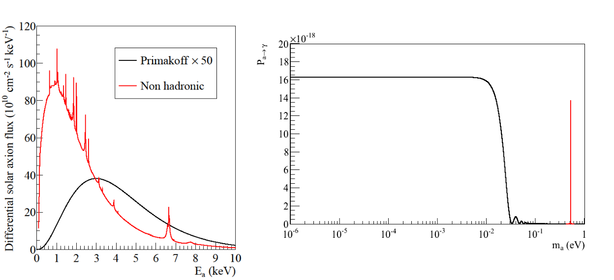
Although the non-hadronic axion emission could be larger in the solar core, only the Primakoff processes have been taken into account in this work because is more reliable to suppose the same processes involving the generation and detection of axions. Also, astrophysical constrains on are more restrictive than the limits that could be in principle reached with helioscopes. The solar axion flux is well established due to the detailed description of the Solar Model. The probability of the axion to photon conversion inside a strong magnetic field was introduced by van Bibber. In the helioscope technique the sensitivity to the axion mass is given by the conversion probability, which is constrained to small axion masses if the magnet bores are under vacuum (see figure 2 right). However, the coherence can be restored to higher axion masses using a buffer gas inside the magnet bores.
The most representative experiment in the helioscope technique is the CAST (CERN Solar Axion Telescope) experiment, looking for solar axions since 2003 and being the most sensitive helioscope so far. CAST makes use of a decommissioned LHC dipole magnet with a length of 9.26 m and a magnetic field up to 9 T. The magnet is mounted on a movable platform which allows to tracking the Sun h two times per day, during sunrise and sunset (see figure 3). The magnet is composed by two bores with a total of four detectors placed at the magnet bore ends. The axion signal would be an excess of X-rays while the magnet is pointing the Sun and low background X-ray detectors are mandatory.

The CAST experiment is composed of several additional systems required for the data taking. The magnet operates at a nominal temperature of 1.8 K and a cryogenic cooling system is required. Also, a vacuum system is installed around the magnet bores in order to increase the transparency for the X-rays from the axion conversion and to isolate the magnet from the environment. The movement of the magnet is controlled by a tracking system program which allows to point the Sun automatically. Also, a gas system is installed with the purpose of filling the magnet bores with a buffer gas in small steps. Finally, the monitoring of all the systems is performed by the slow control.
The CAST research program can be divided into two phases, the first one with vacuum inside the magnetic bores and a second phase with buffer gas. The Phase I data taking period was performed during 2003 and 2004, reaching a limit on the coupling constant of GeV-1 at a 95 of C.L., for axion masses eV.
During the Phase II, from 2005 to 2006, the magnet was filled with 4He, providing an experimental limit of GeV-1 at a 95 of C.L. for axion masses eV. The 3He phase started in 2008 and ended in 2011, scanning axion masses of eV and obtaining an experimental limit of GeV-1 for eV and GeV-1 for eV at a 95 of C.L. CAST crossed first time the KSVZ benchmark model, one of the most favored in the theory. Although CAST finished its original research program in 2011, the data taking period has been extended. During 2012 the 4He phase was revisited, improving the previous limit in a narrow mass range. In 2013 CAST started a new data taking campaign revisiting the vacuum phase, motivated by the improvement of the background levels of the X-rays detectors and an improvement of the sensitivity is expected.
Three different kind of X-rays detectors have been working at CAST since the beginning of the experiment: a Charge Coupled Device (CCD) on the focal plane of an X-ray telescope, a Time Projection Chamber (TPC) covering two magnet bores on the Sunset side and different types of Micromegas (MICRO MESh GAseous Structure) detectors that have been taking data in the Sunrise side and more recently in the Sunset side.
The Micromegas detectors were developed by Giomataris in 1996. Micromegas are gaseous ionization detectors with two different regions separated by a mesh: the conversion region and the amplification region. In the conversion region the interacting particles ionize the gas generating primary charges, in this region an electric field is applied and the electrons are drifted to the amplification region. Here the avalanche of the primary electrons occurs, due to the strong electric field present in the gap (of m), generating two readable signals: one in the mesh that provides time resolution and another in the anode readout which confers spatial resolution to the detectors. A scheme of the working principle of the Micromegas detectors is shown in figure 4.
Micromegas is a demanding technology which has experienced a technological evolution in the manufacturing process, from the classical Micromegas to the bulk and microbulk technologies. The CAST experiment has been a demanding test bench for these different manufacturing techniques. The latest microbulk technology is the one which shows the better performance and the lower intrinsic radiopurity. Three of the four detectors currently installed at CAST are of this type.
The design of the microbulk Micromegas detectors installed at CAST during 2011 has been carefully selected for axion searches. The detector anode is made of interconnected square pads which leads to a 2-dimensional strip readout of strips with a pitch of 550 m and an effective area of about mm2. The cathode is made of aluminized mylar of about 5 m thick, glued to a circular aluminum strongback, which is attached to the vacuum side of magnet. The body of the detector is made of Plexiglas, the chamber and thus the conversion volume has 30 mm height. The Micromegas is glued to a Plexiglas base called raquette which has a circular shape in the detector area and a thin neck for the strips connections to the electronics. The gas in the chamber is an Ar + iC4H mixture, working at a pressure of 1.4 bar. The detectors are placed at the magnet bore ends covering the entire aperture of 14.52 cm2. Although Sunrise and Sunset detectors have different shielding designs, both of them are mainly composed by 5 mm of copper in the innermost part, 25 mm of archaeological lead and 2 mm of cadmium foil at the end, covered by polyethylene layers.
The acquisition of the different readouts of the Micromegas detectors at CAST is performed by a Labview based program. The mesh pulse is digitized by a Matacq board and the anode readout is acquired by the Gassiplex font end electronics. The data analysis is done by a dedicated software based on C++ and ROOT. For the mesh signal a pulse shape analysis is made, this leads to the definition of different observables. For the strips readout a cluster analysis is performed, that allows the definition of different parameters related with the shape of the event.
In a second stage, the discrimination of the X-ray like events is performed. For this purpose, the distribution of the background events is compared with the distribution of the 55Fe calibration events (see figure 5 left). The discrimination method has been developed computing the log-odds distribution of different observables for calibration and background events. It allows to define a cut value in which a certain number of events are accepted (see figure 5 right), that leads to the definition of the software efficiency.

Using this discrimination method, the data of the Micromegas detectors at CAST during 2011 have been analyzed. The discrimination capabilities of the detectors are strongly dependent on the detector performance. As it was shown in chapter 4 the Sunrise detector shows an excellent performance in comparison with the ones installed in the Sunset side and thus its potential for axion discovery is higher. An optimization of the software efficiency and the background level of the detectors has been performed, in which the figure of merit of the detectors has been maximized. The background and tracking levels of the Micromegas detectors during 2011 are presented in table 1. As shown, both levels are compatible, in addition the occurrence of the events during background and tracking are compatible with the expected Poissonian.
| Detector | Number of | Background level | Tracking level |
|---|---|---|---|
| trackings | c cm-1s-1keV-1 | c cm-1s-1keV-1 | |
| Sunrise | 46 | (6.09 0.10)10-6 | (5.71 0.55)10-6 |
| Sunset1 | 45 | (5.96 0.10)10-6 | (6.14 0.57)10-6 |
| Sunset2 | 45 | (6.83 0.11)10-6 | (7.58 0.63)10-6 |
In order to distinguish the presence of an axion signal in the Micromegas data, an unbinned likelihood method has been developed. In a first stage, for every axion mass, the log-likelihood is computed for several values of the coupling constant , in which the minimum and the standard deviation are extracted. If the minimum is compatible with the absence of signal (see figure 6), an upper limit to the coupling constant may be derived.

After discarding a possible axion signal, a limit on the axion to photon coupling is extracted. An upper limit to the coupling constant for a given axion mass has been calculated by integrating the Bayesian probability at a 95 of C.L. The derived limit for the 2011 Micromegas data at the CAST experiment is shown in figure 7.
In order to estimate the systematic uncertainties, the determination of the effective coherence length has been considered as the main source of error. Indeed, the 3He dynamics inside the magnet bores has a complex behavior, due to hydrostatic and convection effects at a cryogenic temperature. In order to calculate the effective length, a detailed study of the density profile of the 3He has been performed using CFD11 1 Computational Fluid Dynamics simulations. The effective coherence length has been parameterized for a given pressure inside the magnet bores. However, the profile density along the magnet cannot be measured and the simulation has some uncertainties. Two extreme cases have been taken into account in order to estimate the systematics: one considering all the magnet length (9.26 m) as the coherence region and another using a conservative scenario for the coherence region. The average values of the coupling limit for the nominal analysis and the ones described above for the systematics, for eV, have been computed:
| (1) |
Using the unbinned likelihood method, the data of the 3He phase of the CAST experiment, from 2008 to 2011, have been computed and a coupling limit has been extracted. The results are shown in figure 8.
CAST finished the 3He phase extending the axion search up to eV, crossing first time the KSVZ benchmark (E/N=0) model, one of the most favored in the theory. Although there was no axion signal, CAST is currently rescanning the vacuum phase with an enhanced sensitivity, due to the improved background level in the Micromegas detectors.
CAST microbulk Micromegas exploit different techniques in order to improve its background level: the intrinsic radiopurity; the improvements in the manufacturing process; the event discrimination and the shielding strategy. These strategies have been described in chapter 6. In order to understand the origin of the background level of the detectors, different special set-ups have been developed: one in the LSC and another in the Zaragoza laboratory. For the underground measurements, the muon flux is highly suppressed and its contribution to the background can be considered negligible, with the proper shielding the background is reduced to a c cm-2 keV-1 s-1 level. Moreover, different contributions to the background have been measured in this set-up, like the Al strongback or the effect of the 222Rn (see figure 9 left). On the other hand, the measurements performed at surface level were crucial in order to measure the contribution of the muons to the final background and an important test bench in order to develop the DAQ with the novel AFTER front end electronics. These special set-ups together with the simulations (see figure 9 right) have set the roadmap to the different upgrades developed for the Micromegas detectors at CAST.

Following the low background strategies developed for the Micromegas detectors, the Sunset detectors were upgraded during 2012. A new shielding design was proposed with an inner copper shielding of 10 mm and a lead shielding of 100 mm (see figure 10 left), which has been extended along the magnet bore pipes. Moreover, the connection to the magnet bores is done by a 10 mm thick copper pipe, which has an inner PTFE coating with a thickness of 2.5 mm in order to attenuate the copper fluorescence at 8 keV. Additionally, two plastic scintillators were installed around the shielding (see figure 10 right) in order to discriminate events related with muons. Also, during 2013 the novel AFTER front-end electronics for the strip readout were installed, which lead to a better discrimination of the background events.
During the 2014 CAST data taking campaign an X-ray focusing device was installed in the Sunrise side, with a Micromegas detector in its focal plane (see figure 11). The Sunrise Micromegas detector has a novel design, the body and the chamber of the detector is made of 20 mm thick radiopure copper and all the gaskets are made of PTFE. Following the Sunset design, the shielding has a thickness of 100 mm of lead, which is extended along the magnet bore pipe and a plastic scintillator is installed on the top for the rejection of the events induced by muons. Furthermore a new Micromegas detector has been manufactured for the new line, being the one with the better performance working at CAST with a 13 of FWHM in the 5.9 keV peak and an excellent spatial resolution and homogeneity of the gain in the active area.
The upgrades of the Micromegas detectors at CAST have led to a reduction of the background level down to c cm-2 keV-1 s-1. Moreover, the new XRT+Micromegas line in the CAST experiment has set a milestone in axion research. CAST will finish the rescanned vacuum phase at the end of 2015 improving its previous limit to an expected value of GeV-1, due to the reduction of the background levels of the detectors and the new XRT. However, the discovery potential of CAST is limited by the size of the magnet. In order to scan a wider region of the parameter space the IAXO experiment has been proposed.
Beyond CAST a new generation helioscope with a improved sensitivity, specifically built for axion and ALPs searches, has been proposed: IAXO-the International AXion Observatory. It will enhance the helioscope technique by exploiting all the singularities of CAST, implemented into a large superconducting toroidal magnet, together with X-ray optics and ultra-low background detectors attached to the magnet bore ends. IAXO detectors have a goal of background levels of c cm-2 keV-1 s-1 (see figure 12) and down to if possible.
The new system (Micromegas+XRT) at CAST, can be considered as a IAXO pathfinder, being an important milestone for the technical design phase of IAXO. However, the final background is around one order of magnitude above the levels required for IAXO. In this way, the design of a D0 detector for IAXO has been proposed, it will feed by the low background techniques developed until now and also new research lines have been proposed, such as the improvement of the muon veto coverage, new thin cathode windows, new gas mixtures, the novel AGET front end electronics and resistive Micromegas.
Due to a dedicated magnet, optics and ultra-low background detectors, IAXO will surpass the sensitivity of CAST in more than one order of magnitude (see figure 13). IAXO will be sensitive to coupling constants of about GeV-1, entering into an unexplored parameter space area and by first time in a favored region for axions and ALPs.
IAXO could directly measure the solar flux of axions produced by non-hadronic processes, for the first time with sensitivity to relevant values. However, in this case the reduction of the low energy threshold in the detectors and the increment of the efficiency at low energies will be crucial. On the other hand, the huge magnet required for IAXO offers excellent possibilities to host relic dark matter searches of axions and ALPs and the use of a dish antenna and resonant cavities are under study.
The haloscope technique consists in a tunable microwave-cavity in a strong magnetic field coupled to an ultra-low-noise microwave sensor. CDM axions and ALPs may convert into photons in the microwave regime with an enhanced probability if the resonant frequency of the cavity matches the axion energy. A directional effect on the detection could be observed by the use of long thin cavities properly tuned. This case has been studied in chapter 8 and could provide a strong identificative signature of the direction of the CDM axions. The expected sensitivity of this kind of resonant cavities is shown in figure 14.
The use of thin cavities inside long magnets for relic axion detection is particularly appealing, because it could be realized in the near future, given that this type of magnets are already used by the axion community in experiments looking for solar axions, like CAST. Moreover, the huge magnet required for IAXO offers excellent possibilities and the hosting of this kind of cavities is under study.
Chapter 10 Resumen y conclusiones
Los axiones son partículas pseudo-escalares propuestas en una extensión del Modelo Estándar (SM) como una solución al problema the CP en las interacciones fuertes. La teoría precide una violación de CP en las interacciones fuertes que no ha sido observada experimentalmente. La solución más convincente a este problema fue propuesta por Peccei y Quinn en 1977, en ella se introduce una simetría global y quiral que se rompe espontáneamente en la escala de energía de la simetría. De esta manera se soluciona el problema CP dinámicamente y aparece el axión, como en bosón pseudoescalar de Nambu-Goldstone de la nueva simetría.
La solución de Peccei-Quinn fija algunas propiedades de los axiones como su masa y su constante de acoplo, que están relacionadas con la escala de energía de la nueva simetría, . Los axiones pueden interacturar con gluones, fotones y fermiones. Sin embargo, el acoplo más interesante es el de axión-fotón, que es genérico para todos los modelos.
Aún cuando los axiones son las partículas mejor motivadas en la teoría, también existe la categoría de partículas tipo axión (ALPs) o más genéricamente WISP (Weakly Interacting Slim Particles). Las cuales comparten la misma fenomenología que el axión, siendo partículas ligeras que se acoplan a dos fotones. Las ALPs emergen de extensiones del SM donde una nueva simetría se rompe a altas escalas de energía, también aparecen en la teoría de cuerdas al igual que el axión. Sin embargo en este caso la constante de acoplo no está relacionada con su masa, de esta manera las ALPs pueden encontrarse en extensas regiones del espacio de parámetros .
Tanto los axiones como las ALPs podrían haberse producido en un Universo primitivo mediante mecanismos no térmicos, como el realineamiento del vacío o el decaimiento de los defectos topológicos. Siendo partículas neutras que interaccionan débilmente con la materia, tanto los axiones como las ALPs son atractivos candidatos a Materia Oscura (DM), que podrían explicar separadamente toda la cantidad de DM en el Universo. Sin embargo las propiedades de los axiones y de las ALPs están restringidas debido a consideraciones provenientes de la astrofísica y de la cosmología, ya que podrían tener un papel importante en la evolución estelar. Por otra parte diferentes observaciones experimentales podrían ser interpretadas como un indicio de axiones o ALPs. Como la excesiva transparencia del Universo a fotones de alta energía o el enfriamiento anómalo de las Enanas Blancas.
Diferentes técnicas han sido desarrolladas en la búsqueda de axiones: helioscopios que buscan axiones solares, haloscopios que buscan axiones primigéneos parte de la DM y experimentos de regeneración en los que los axiones podrían ser generados y detectados en el laboratorio. Todas ellas están basadas en el effecto Primakoff, donde los axiones podrían ser convertidos en fotones en presencia de campos electromagnéticos.
La técnica del helioscopio, la cual es el tema principal de este trabajo, fue propuesta por Sikivie en 1983, en ella se utiliza al Sol como una poderosa fuente de axiones. Los axiones solares podrían generarse en el núcleo solar en los fuertes campos eléctricos de plasma solar por medio del efecto Primakoff inverso. Además, la emisión de axiones por procesos adicionales como Bremsstrahlung de axiones, Compton y axio-desexcitación podría ser considerablemente más importante que la de los procesos Primakoff. Estos axiones podrían ser reconvertidos en fotones en presencia de fuertes campos magnéticos mediante el efecto Primakoff (ver figura 1). Estos fotones, que están en el rango de energía de los rayos-X (ver la parte izquierda de la figura 2), podrían ser detectados en detectores de rayos-X colocados en los extremos del imán.
Aunque la emisión de axiones solares mediante procesos no hadrónicos podría ser más importante, en este trabajo solamete se tienen en cuenta los procesos Primakoff. Debido a que es más consistente suponer los mismos procesos en la generación y detección de axiones. Además, las restricciones provenientes de la astrofísica en son más restrictivas que los límites que en principio pueden ser alcanzados por los helioscopios. El flujo de axiones solares está bien establecido debido a la detallada descripción del Modelo Solar. Por otra parte la probabilidad de conversión axión-fotón dentro de fuertes campos magnéticos fue introducida por van Bibber. En la técnica del helioscopio, la sensibilidad a la masa del axión viene dada por la probabilidad de conversión, la cual está restringida a masas pequeñas en el caso de que el imán esté en vacío (ver la parte derecha de la figura 2). Sin embargo, la coherencia puede ser restaurada a mayores masas de axiones utilizando gas de buffer dentro del imán.
El mayor exponente dentro de la técnica de los helioscopios es el experimento CAST (CERN Solar Axion Telescope), que busca axiones solares desde 2003, siendo el helioscopio más sensible hasta la fecha. Para ello utiliza un imán obsoleto del LHC de tipo dipolo, con una longitud de 9.26 m y con campos magnéticos hasta 9 T. El imán está montado en una plataforma móvil, la cual permite apuntar al Sol durante h dos veces al día, durante la salida y la puesta del Sol (ver figura 3). El imán está compuesto por dos cavidades magnéticas con un total de cuatro detectores de rayos-X colocados en sus extremos. La señal de axiones sería un exceso de rayos-X cuando el imán apunta al Sol y el uso de detectores de bajo fondo es fundamental.
El experimento CAST está compuesto por varios sistemas adicionales que se requieren para la toma de datos. El imán opera a una temperatura nominal del 1.8 K, para lo que se requiere un sistema criogénico de enfriamiento. También un sistema de vacío ha sido instalado alrededor the las cavidades del imán, con el propósito de incrementar la transparencia de los rayos-X provenientes de los axiones y para aislar el imán del ambiente. El movimiento del imán se controla mediante un programa de seguimiento, el cual permite apuntar automáticamente al Sol. Además, un sistema de gas ha sido instalado con el propósito de rellenar las cavidades del imán con un gas de buffer en pequeñas cantidades. Finalmente todos los sistemas son monitorizados mediante el slow control.
El programa de investigación de CAST se puede dividir en dos fases, la primera con vacío dentro de las cavidades del imán y una segunda fase utilizando gas de buffer. El periodo de toma de datos de la Fase I, se realizó durante 2003 y 2004, obteniendo un límite en la constante de acoplo de GeV-1 a un 95 de nivel de confianza (C.L.), para masas de axiones eV.
Durante la Fase II, de 2005 a 2006 el imán se rellenó de 4He, obteniendo un límite de GeV-1 con un 95 de CL, para masas de axión eV. Mientras que la fase de 3He se inició en 2008 y finalizó en 2011, donde se escanearon masas de axiones eV, obteniendo un límite en la constante de acoplo de GeV-1 para eV y GeV-1 para eV con un 95 de C.L. Cruzando por primera vez el modelo de referencia KSVZ, uno de los más favorecidos por la teoría. Aunque CAST finalizó su programa de investigación en 2011, la toma de datos ha sido ampliada. En 2012 la fase de 4He fue reescaneada, mejorando el límite anterior en una estrecha región. En 2013 una nueva fase de vacío se inició en CAST, motivada por la mejora del nivel de fondo de los detectores, donde se espera una mejora en la sensibilidad del experimento.
Tres tipos diferentes de detectores han operado en CAST desde el comienzo del experimento: un dispositivo de carga acoplada (CCD) en el plano focal de un telescopio de rayos-X, una cámara de proyección temporal (TPC) que cubría las dos cavidades del imán en el lado de la puesta del Sol, que operó hasta 2006, finalmente diferentes tipos de detectores Micromegas (MICRO MEsh GAseous Structure) han estado tomando datos en el lado de la salida del Sol y más recientemente en el lado de la puesta del Sol.
Los detectores Micromegas fueron desarrollados por Giomataris en 1996. Son del tipo de ionización con dos regiones separadas por una rejilla o mesh: la región de conversión y la región de amplificación. En la región de conversión las partículas interaccionantes ionizan el gas, generando cargas primarias, en esta región está presente un campo eléctrico debido al cual los electrones se derivan hacia la región de amplificación. En la cual se produce la avalancha de los electrones primarios, debido al gran campo eléctrico presente en este gap (de unos m), generando dos señales medibles: una en la mesh, que proporciona resolución espacial y otra en el plano de lectura del ánodo, la cual confiere resolución espacial a los detectores. Un esquema sobre el principio de trabajo de los detectores Micromegas se muestra en la figura 4.
Los detectores Micromegas son una tecnología en alza, la cual ha experimentado una evolución tecnológica en el proceso de fabricación, desde las Micromegas clásicas hasta las tecnologías bulk y microbulk. El experimento CAST ha sido un demandante banco de pruebas para estas diferentes técnicas de fabricación donde la nueva tecnología microbulk es la que muestra un mejor rendimiento y la mayor radiopureza. Tres de los cuatro detectores instalados en CAST actualmente son de este tipo.
El diseño de los detectores Micromegas del tipo microbulk instalados en CAST durante 2011 ha sido cuidadosamente seleccionado para la búsqueda de axiones. El ánodo del detector esta hecho de pistas cuadradas interconectadas. Esto lleva a un plano de lectura bidimensional de de pistas con una distancia entre ellas de 550 m y un área efectiva de mm2. El cátodo esta hecho de mylar aluminizado de unos 5 m de grosor, pegado a una rejilla de aluminio de forma circular, la cual se coloca al lado de vacío del imán. El cuerpo del detector está hecho de plexiglass, donde la cámara y la región de conversión tienen una altura de 30 mm. La Micromegas está pegada a una base de plexiglass llamada raqueta que tiene una forma circular en la región del detector y un cuello estrecho para el paso de las conexiones de las pistas a la electrónica. El gas en la cámara es una mezcla de Ar + iC4H, a una presión de 1.4 bares. Los detectores se colocan en los extremos de las cavidades del imán, cubriendo toda la apertura de 14.52 cm2. Aunque los detectores del la salida y la puesta de Sol tienen diferentes diseños de blindaje, ambos están compuestos principalmente de 5 mm de cobre en la parte más interna, 25 mm de plomo arqueológico y una lámina de 2 mm de cadmio en la parte mas externa, cubierto por diferentes capas de polietileno.
La adquisición de los diferentes planos de lecturas de los detectores Micromegas en CAST se realiza mediate un programa basado en Labview. El pulso de la mesh se digitaliza mediante una tarjeta Matacq y el plano de lectura del ánodo se adquiere mediante las tarjetas Gassiplex. El análisis de los datos se realiza mediante un programa dedicado, basado en C++ y en ROOT. Para la señal de la mesh se realiza un análisis de la forma del pulso, lo cual conlleva la definición de diferentes observables. Para el plano de lectura del ánodo se realiza un análisis por clusters, lo cual permite la definición de diferentes parámetros relacionados con la forma del evento.
En una segunda etapa, se procede a la discriminación de los eventos tipo rayos-X. Para ello de compara la distribución de los eventos de fondo con las de los eventos de la calibración diaria con 55Fe (ver parte izquierda de la figura 5). De esta manera se ha desarrollado un método de discriminación, computando la distribución de log-odds de diferentes observables, tanto para eventos de calibraciones como para los de fondo. Esto permite definir un valor de corte para el cual un cierto número de eventos son aceptados (ver parte derecha de la figura 5), lo cual conlleva la definición de una eficiencia de software.
Utilizando este método de discriminación, se han analizado los datos de los detectores Micromegas en CAST durante 2011. El poder de discriminación de los detectores es fuertemente dependiente de la calidad del detector. Como se ha descrito en el capítulo 4, el detector de la salida del Sol muestra unas cualidades excelentes, en contraste con los detectores instalados en el lado de la puesta del Sol y su potencial para el descubrimiento de axiones es mayor. Se ha realizado una optimización de la eficiencia de software en conjunto con el nivel de fondo de los detectores, de esta manera se ha maximizado la figura de mérito de los detectores y consecuentemente su potencial para el descubrimiento de axiones. Los niveles de fondo y durante el seguimiento al Sol para los detectores Micromegas en 2011 se muestran en la tabla 1. Como se puede observar ambos niveles son compatibles, además se ha comprobado que la ocurrencia de eventos tanto de fondo como de seguimiento al Sol sigue distribución de Poisson.
| Detector | Number of | Background level | Tracking level |
|---|---|---|---|
| trackings | c cm-1s-1keV-1 | c cm-1s-1keV-1 | |
| Sunrise | 46 | (6.09 0.10)10-6 | (5.71 0.55)10-6 |
| Sunset1 | 45 | (5.96 0.10)10-6 | (6.14 0.57)10-6 |
| Sunset2 | 45 | (6.83 0.11)10-6 | (7.58 0.63)10-6 |
Con el objetivo de discriminar la presencia de una señal se ha desarrollado un método unbinned likelihood. En una primera fase, para cada masa de axión, se calcula la log-likelihood para diferentes valores de la constante de acoplo , donde se extrae el mínimo y la desviación estándar. Si el mínimo es compatible con la ausencia de señal (ver figura 6), se puede extraer un límite en la constante de acoplo.
Después de descartar una posible señal de axiones, se extrae un límite en la constante axión-fotón. Donde se ha calculado un límite superior para una masa de axión dada mediante la integración de la probabilidad Bayesiana con un 95 de C.L. El límite extraído para los datos de los detectores Micromegas durante la campaña de 2011 se muestra en la figura 7.
Con el objetivo de estimar el error sistemático en el límite extraído se considera la determinación de la longitud efectiva de coherencia como la mayor fuente de error. La dinámica del 3He en las cavidades del imán tiene un comportamiento complejo debido a efectos hidrostáticos y de convección a una temperatura criogénica. Con el objetivo de calcular la longitud efectiva del imán se ha realizado un estudio detallado del perfil de densidades dentro del imán utilizando simulaciones CFD11 1 Computación de Dinámica de Fluidos. De esta manera la longitud de coherencia en el imán ha sido parametrizada para una presión dada. Sin embargo, el perfil de densidades a lo largo del imán no puede ser medido y la simulación tiene ciertas incertidumbres. Dos casos extremos se han tenido en cuenta para estimar el error sistemático en la constante de acoplo: uno de ellos considerando como longitud de coherencia toda la longitud del imań (9.26 m) y otro utilizando un escenario conservador para la región de coherencia. El valor promedio de las constantes de acoplo para el análisis nominal y para los descritos anteriormente para el cálculo de sistemáticos, en el rango de masas eV, se muestran a continuación:
| (1) |
Utilizando el método unbinned likelihood se han analizado los datos de toda la fase de de 3He, de 2008 a 2011, extrayendo un límite en la constante de acoplo. Los resultados se muestran en la figura 8.
CAST finalizó la fase de 3He extendiendo la búsqueda de axiones hasta eV, cruzando por primera vez el modelo de referencia KSVZ , uno de los más farorecidos en la teoría. Aunque no hubo ninguna señal de axiones, CAST actualmente está reescaneando la fase de vacío con una sensibilidad mejorada, debido a la reducción del nivel de fondo en los detectores Micromegas.
Los detectores Micromegas del tipo microbulk explotan diferentes técnicas para la reducción del nivel de fondo: la radiopureza intrínseca; las mejoras en el proceso de fabricación; la discriminación de eventos de fondo y el blindaje. Estas estrategias han sido descritas en el capítulo 6. Con el propósito de entender el origen del fondo de los detectores se han desarrollado diferentes montajes: uno en el LSC y otro en el laboratorio de Zaragoza. Para las medidas bajo tierra, el flujo de muones está altamente suprimido y su contribución se puede considerar despreciable. Con el blindaje adecuado el fondo se reduce a un nivel de c cm-2 keV-1 s-1 (ver parte izquierda de la figura 9). Además diferentes contribuciones al fondo de los detectores han sido medidas, como la del cátodo de aluminio o el efecto del 222Rn en el montaje. Por otra parte, las medidas realizadas en superficie fueron cruciales para medir la contribución de los muones al fondo de los detectores y un importante banco de pruebas para el desarrollo de la adquisición con la nueva electrónica AFTER. Estos montajes especiales junto con las simulaciones (ver parte derecha de la figura 9) marcaron la hoja de ruta para las diferentes mejoras desarrolladas para los detectores Micromegas en CAST.
Siguiendo las estrategias de fondo desarrolladas para los detectores Micromegas, los detectores de la puesta de Sol fueron mejorados en 2012. Con un nuevo diseño del blindaje con un capa interna de 10 mm de cobre y una capa externa de 100 mm de plomo (ver parte izquierda de la figura 10), la cual se ha extendido a través de las tuberías hacia las cavidades magnéticas. Además, la conexión hacia estas cavidades se realiza mediante una tubería de cobre de 10 mm de grosor con un recubrimiento de PTFE de 2.5 mm para atenuar la fluorescencia del cobre a 8 keV. También se han instalado dos centelleadores plásticos cubriendo en blindaje (ver parte derecha de la figura 10), con el propósito de discriminar eventos relacionados con muones. Además, durante 2013 se instaló la nueva electrónica AFTER para el plano de lectura del ánodo, que conlleva a una mejor discriminación de los sucesos de fondo.
Durante la toma de datos de CAST correspondiente al año 2014, se ha instalado en el lado de la salida del Sol un nuevo telescopio de rayos-X con una Micromegas en su plano focal (ver figura 11). El detector Micromegas de la salida del Sol tiene un nuevo diseño, en el cual la raqueta y la cámara están compuestas por cobre radiopuro de un grosor de 20 mm, además todas las juntas están hechas de PTFE. También siguiendo el diseño de los detectores de la puesta de Sol, el blindaje de plomo tiene un grosor de 100 mm, el cual se extiende a través de la tubería hacia el imán, también se ha instalado un centelleador plástico encima del blindaje para discriminar los eventos inducidos por muones. Además, un nuevo detector Micromegas se ha fabricado para la nueva línea, siendo uno de los detectores con las mejores cualidades instalados en CAST, con un 13 de resolución FWHM en el pico de 5.9 keV y una excelente resolución espacial y homogeneidad de la ganancia en la zona activa.
Las mejoras de los detectores Micromegas en el experimento CAST han conllevado una reducción del fondo a unos niveles de c cm-2 keV-1 s-1. Además, la nueva línea del XRT+Micromegas de CAST supone un hito en la investigación de axiones. CAST acabará la nueva fase de vacío en 2015 mejorando el anterior límite, debido a la reducción del fondo de los detectores y el nuevo telescopio de rayos-X. Donde se espera una reducción del límite en la constante de acoplo a valores sobre GeV-1. Sin embargo, la sensibilidad de CAST está limitada principalmente por el tamaño del imán. Con el propósito de escanear una región más extensa del espacio de parámetros , se ha propuesto el experimento IAXO.
Más allá de CAST, se ha propuesto un helioscopio de nueva generación, con una sensibilidad mejorada y específicamente construido para la búsqueda de axiones y ALPs: IAXO-el Observatorio Internacional de Axiones. El cual mejorará la técnica del helioscopio explotando todas las peculiaridades de CAST, implementadas en un gran imán toroidal superconductor, junto con nuevas ópticas de rayos-X y detectores de ultra-bajo fondo situados en los extremos del imán. Con el objetivo de alcanzar niveles de fondo de c cm-2 keV-1 s-1 (ver figura 12) y hasta si es posible.
El nuevo sistema (Micromegas+XRT) de CAST, puede ser considerado como pionero de IAXO, siendo un hito importante para la fase de diseño técnico. Sin embargo, el nivel de fondo en CAST está un orden de magnitud por encima de los niveles requeridos para IAXO. De este modo se ha propuesto el desarrollo de un detector D0 para IAXO, el cual se proveerá de las técnicas de bajo fondo desarrolladas hasta ahora, además nuevas mejoras y líneas de investigación han sido propuestas, tales como: mejoras en la cobertura de los vetos de muones, nuevas ventanas para el cátodo, nuevas mezclas de gases, la novedosa electrónica AGET y Micromegas resistivas.
Gracias a un imán dedicado, óptica y detectores de ultra-bajo fondo, IAXO superará la sensibilidad de CAST en más de un orden de magnitud (ver figura 13). Siendo sensible a constantes de acople entorno a GeV-1. Entrando en un área inexplorarada del espacio de parámetros y por primera vez en una región favorable para axiones y ALPs.
IAXO podría medir directamente el flujo de axiones solares producidos en procesos no hadrónicos y ser por primera vez sensible a valores de relevantes. Sin embargo, en este caso será crucial la reducción del umbral de energía de los detectores y el aumento de eficiencia a bajas energías. Por otra parte, el inmenso imán que se requiere para IAXO ofrece excelentes posibilidades para albergar búsquedas de axiones y ALPs componentes de DM, de esta forma se están estudiando el uso de una antena parabólica (dish antenna) y cavidades resonantes.
La técnica del haloscopio consiste en una cavidad de microondas ajustable dentro de un fuerte campo magnético, acoplada a sensores de microondas de ultra-bajo fondo. Axiones y ALPs CDM podrían convertirse en fotones en el régimen de las microondas con una probabilidad mejorada en el caso de que la frecuencia de resonancia de la cavidad coincida con la energía del axión. Se podría observar un efecto direccional mediante el uso de cavidades estrechas y largas apropiadamente ajustadas. Este caso ha sido estudiado en el capítulo 8 y podría proporcionar una fuerte señal de identificación de los axiones CDM. La sensibilidad de este tipo de cavidades resonantes ha sido estudiada y se muestra en la figura 14.
El uso de cavidades estrechas dentro de imanes largos para la detección de axiones reliquia es un caso particularmente atractivo, ya que se podría realizar en un futuro próximo, dado que este tipo de imanes están siendo utilizados en la comunidad de axiones, en experimentos que buscan axiones solares, como CAST. Además, el enorme imán que se requiere para IAXO ofrece excelentes posibilidades y se está estudiando la posibilidad de albergar de cavidades resonantes en el rango de las microondas.
References
- [1] R. D. Peccei and Helen R. Quinn. CP Conservation in the Presence of Pseudoparticles. Phys. Rev. Lett., 38(25):1440 (1977).
- [2] S. Weinberg. The U(1) problem. Phys. Rev. D 11(12):3583, (1975).
- [3] G. ’t Hooft. Symmetry Breaking through Bell-Jackiw Anomalies. Phys. Rev. Lett. 37(1):8, (1976).
- [4] G. ’t Hooft. Computation of the quantum effects due to a four-dimensional pseudoparticle. Phys. Rev. D 14, (12):3432 (1976).
- [5] V. Baluni. CP-nonconserving effects in quantum chromodynamics. Phys. Rev. D 19, 2227 (1979).
- [6] C. A. Baker et al. Improved experimental limit on the electric dipole moment of the neutron. Phys. Rev. Lett. 97, 131801 (2006).
- [7] R. D. Peccei and H. R. Quinn. CP conservation in the Presence of Instantons, Phys. Rev. Lett. 38, 1440 (1977).
- [8] R. D. Peccei and H. R. Quinn. Constraints imposed by CP conservation in the presence of instantons. Phys. Rev. D 16, 1791 (1977).
- [9] G. Raffelt. Astrophysical axion bounds diminished by screening effects. Phys. Rev. D 33, 897 (1986).
- [10] R. D. Peccei and H. R. Quinn. Constraints imposed by CP conservation in the presence of pseudoparticles. Phys. Rev. D 16(6), 1791 (1977).
- [11] M. A. Shifman, A. I. Vainshtein and V. I. Zakharov. Can confinement ensure natural CP invariance of strong interactions? Nuclear Physics B 166(3):49, (1980).
- [12] J. E. Kim. Weak-Interaction Singlet and Strong CP Invariance. Phys. Rev. Lett. 43(2):103, (1979).
- [13] M. Dine, W. Fischler and M. Srednicki. A simple solution to the strong CP problem with a harmless axion. Phys. Lett. B 104(3):199, (1981).
- [14] S. Hannestad, A. Mirizzi, G. Raffelt, and Y. Wong. Neutrino and axion hot dark matter bounds after WMAP-7. JCAP 1008, 001 (2010).
- [15] P. Gondolo and G. Raffelt. Solar neutrino limit on axions and keV-mass bosons. Phys.Rev. D79, (2009) 107301.
- [16] N. Viaux, M. Catelan, P.B. Stetson, G. Raffelt, J. Redondo, A. R. Valcarce and A. Weiss. Neutrino and axion bounds from the globular cluster M5 (MGC 5904). Phys. Rev. Lett. 111, 231301 (2013).
- [17] G. Raffelt, Astrophysical axion bounds. Lect. Notes Phys. 741, 51 (2008).
- [18] S. Chandrasekhar. The Highly Collapsed Configurations of a Stellar Mass. Monthly Notices of the Royal Astronomical Society 91, 456 (1931).
- [19] G. Raffelt. Stars as Laboratories for Fundamental Physics: The astrophysics of neutrinos, axions, and other weakly interacting particles. The University of Chicago Press, Chicago & London (1996).
- [20] PLANCK Collaboration PLANCK 2013 results. XVI. Cosmological parameters arXiv:1303.5076.
- [21] P. Sikivie. Axion cosmology. Lect.Notes Phys. 741, 19 (2008).
- [22] O. Wantz and E. P. S. Shellard. Axion Cosmology Revisited. Phys. Rev. D 82, 123508 (2010).
- [23] J. Jaeckel and A. Ringwald. The Low-Energy Frontier of Particle Physics. Annual review of Nuclear and Particle Science 60, 405 (2010).
- [24] P. Arias, D. Cadamuro, M. Goodsell, J. Jaeckel, J. Redondo and A. Ringwald. WISPy Cold Dark Matter. JCAP 1206, 013 (2012).
- [25] A. Abramowski et al. HESS Collaboration. Measurement of the extragalactic background light imprint on the spectra of the brightest blazars observed with H.E.S.S. Astron. Astrophys. 550, (2013).
- [26] Fermi-LAT Collaboration. The Imprint of The Extragalactic Background Light in the Gamma-Ray Spectra of Blazars. Science 338, 1190 (2012).
- [27] F. Aharonian et al. HESS Collaboration. A Low level of extragalactic background light as revealed by gamma-rays from blazars. Nature 440, 1018 (2006).
- [28] E. Aliu et al. MAGIC Collaboration Collaboration. Very-High-Energy Gamma Rays from a Distant Quasar: How Transparent Is the Universe?. Science 320, 1752 (2008).
- [29] M. Meyer, D. Horns and M. Raue. First lower limits on the photon-axion-like particle coupling from very high energy gamma-ray observation. Phys.Rev. D87, 035027 (2013).
- [30] J. Isern, S. Catalan, E. García-Berro, M. Salaris and S. Torres. Axions and the cooling of white dwarf. arXiv:1304.7652 [astro-ph.SR].
- [31] A. H. Corsico et al. The rate of cooling of the pulsating white dwarf star G117-B15A: a new asteroseismological inference of the axion mass. MNRAS 424, 2792 (2012).
- [32] A. H. Corsico et al. An independent limit on the axion mass from the variable white dwarf star R548. JCAP 1212, 010 (2012).
- [33] P. Sikivie. Experimental tests of the invisible axion. Phys. Rev. Lett. 51, 1415 (1983).
- [34] S. DePanfilis et al. Limits on the Abundance and Coupling of Cosmic Axions at 4.5<ma<5.0 eV. Phys. Rev. Lett. 59, 839 (1987).
- [35] C. Hagmann et al. Results from a search for cosmic axions. Phys. Rev. D. 42, 1297 (1990).
- [36] C. Hagmann et al. Results from a high-sensitivity search for cosmic axions. Phys. Rev. Lett. 80(10), 2043 (1998).
- [37] S. J. Asztalos et al. A SQUID-based microwave cavity search for dark-matter axions. Phys. Rev. Lett. 104:041301 (2010).
- [38] M. A. Bershady, M. T. Ressell and M. S. Turner. Telescope search for a 3-eV to 8-eV axion. Phys. Rev. Lett. 66, 1398 (1991).
- [39] D. Grin et al. Telescope search for decaying relic axions. Phys. Rev. D 75, 105018 (2007).
- [40] J. Redondo and A. Ringwald. Light shining through walls. Contemp. Phys. 52, 211 (2011).
- [41] A. Afanasev et al. New Experimental limit on Optical Photon Coupling to Neutral, Scalar Bosons. Phys. Rev. Lett. 101, 120401 (2008).
- [42] C. Robilliard et al. No light shining through a wall: new results from a photoregeneration experiment. Phys. Rev. Lett. 99, 190403 (2007).
- [43] A. S. Chou et al. Search for axion-like particles using a variable baseline photon regeneration technique. Phys. Rev. Lett. 100, 080402 (2008).
- [44] P. Pugnat et al. First results from the OSQAR photon regeneration experiment: No light shining through a wall. Phys. Rev. D 78, 092003 (2008).
- [45] K. Ehret et al. (ALPs Collaboration). New ALPS Results on Hidden-Sector Lightweights. Phys. Lett. B 689 149 (2010).
- [46] M. Betz et al. First results of the CERN Resonant Weakly Interacting sub-eV Particle Search (CROWS). Phis. Rev. D 88, 7 075014 (2013).
- [47] G. Ruoso et al. (BFRT collaboration) Limits on Light Scalar and Pseudoscalar Particles from a Photon Regeneration Experiment. Z. Phys. C 56, 505 (1992).
- [48] G. Cantatore et al. Proposed measurement of the vacuum birefringence induced by a magnetic field on high energy photons. Phys. Lett. B 265, 418 (1991).
- [49] E. Zavattini et al. (PVLAS Collaboration). New PVLAS results and limits on magnetically induced optical rotation and ellipticity in vacuum. Phys. Rev. D. 77, 032006 (2008).
- [50] D. M. Lazarus et al. Search for solar axions. Phys. Rev. Lett., 69(16), 2333, (1992).
- [51] Y. Inoue et al. Search for sub-electronvolt solar axions using coherent conversion of axions into photons in magnetic field and gas helium. Phys. Lett. B536, 18 (2002).
- [52] I. Avignone et al. (SOLAX Collaboration). Experimental Search for Solar Axions via Coherent Primakoff Conversion in a Germanium Spectrometer. Phys. Rev. Lett. 81 5068 (1998).
- [53] A. Morales et al. (COSME Collaborations). Particle Dark Matter and Solar Axion Searches with a small germanium detector at the Canfranc Underground Laboratory. Astropart. Phys. 16, 325 (2002).
- [54] R. Bernabei et al. Search for solar axions by Primakoff effect in NaI crystals. Phys. Lett. B515, 6 (2001).
- [55] Z. Ahmed et al. (CDMS Collaboration). Search for Axions with the CDMS Experiment. Phys. Rev. Lett. 103, 141802 (2009).
- [56] E. Armengaud et al. Axion searches with the EDELWEISS-II experiment. JCAP 11, 067 (2013).
- [57] J. N. Bahcall and M. H. Pinsonneault. What do we (not) know theoretically about solar neutrino fluxes?. Phys. Rev. Lett. 92(12), 121301 (2004).
- [58] J. N. Bahcall et al. Standard solar models and the uncertainties in predicted capture rates of solar neutrinos. Rev. Mod. Phys. 54(3), 767 (1982).
- [59] K. van Bibber, P. M. McIntyre, D. E. Morris and G. G. Raffelt. Design for a practical laboratory detector for solar axions. Phys. Rev. D 39 ,8 2089 (1989).
- [60] J. Redondo. Solar axion flux from the axion-electron coupling. JCAP 1312, 008 (2013).
- [61] A. Serenelli, S. Basu, J. W. Ferguson and M. Asplund. New Solar Composition: The Problem With Solar Models Revisited. Astrophys. J. 705, L123 (2009).
- [62] G. Raffelt and L. Stodolsky. Mixing of the photon with low-mass particles. Phys. Rev. D, 37, (5) 1237 (1988).
- [63] K. Zioutas et al. A decommissioned LHC model magnet as an axion telescope. Nucl. Instrum. and Meth. A425, (3) 480 (1999).
- [64] M. Bona et al. Performance of the first CERN-INFN 10 m long superconducting dipole Prototype for the LHC. Proc. 4th Europ. Particle Accelerator Conf. London, 2289 (1994).
- [65] K. Barth et al. Commissioning and First Operation of the Cryogenics for the CERN Axion Solar Telescope (CAST). AIP Conf. Proc. 710, (CERN-AT-2004-001-ECR) 168 (2004).
- [66] J. I. Collar et al. (CAST Collaboration). CAST: A search for solar axions at CERN. Proc. SPIE (2003).
- [67] Naval observatory vector astrometry subroutines (http://www.usno.navy.mil/).
- [68] K. Zioutas et al. (CAST Collaboration). Minutes of the Technical Design Review of the 3-He system of the CAST experiment. CERN-SPSC-2006-036 (2006).
- [69] K. Zioutas et al. An improved limit on the axion-photon coupling from the cast experiment. JCAP 04, 010 (2007).
- [70] E. Arik et al. (CAST Collaboration). Probing ev-scale axions with cast. JCAP 02, 008 (2009).
- [71] E. Arik et al (CAST Collaboration). CAST search for sub-eV mass solar axions with 3He buffer gas. Phys. Rev. Lett. 107, 261302 (2011).
- [72] E. Arik et al (CAST Collaboration). CAST solar axion search with 3He buffer gas: Closing the hot dark matter gap. Phys. Rev. Lett. 112, 091302 (2014).
- [73] CAST Collaboration. Search for 14.4 keV solar axions emitted in the M1-transition of 57Fe nuclei with CAST. JCAP 0912, 002 (2009).
- [74] CAST Collaboration. Search for solar axion emission from 7Li and D(p,gamma)3He nuclear decays with the CAST gamma-ray calorimeter. JCAP 1003, 032 (2010).
- [75] K. Barth et al. CAST constraints on the axion-electron coupling. JCAP 05, 010 (2013).
- [76] G. Cantatore for the CAST Collaboration. Status report of the CAST Experiment, planning and requests for 2013-2014. CERN-SPSC-2013-027; SPSC-SR-123 (2013).
- [77] M. Arik el al. (CAST Collaboration). New solar axion search in CAST with 4He filling. Submitted in PRL, arXiv:1503.00610.
- [78] J. Altmann et al. Mirror System for the German X-ray Satellite ABRIXAS: I. Flight Mirror Fabrication, Integration, and Testing, in X-Ray Optics, Instruments, and Missions II, Proc. of SPIE 3444, 350 (1998).
- [79] M. Freyberg et al. The MPE X-ray test facility PANTER: Calibration of hard X-ray (15-50 kev) optics. Experimental Astronomy 20, 405 (2005).
- [80] M. Kuster et al. The X-Ray Telescope of CAST. New Journal of Phys. 9, 169 (2007).
- [81] L. Strüder et al. The European Photon Imaging Camera on XMM-Newton: The pn-CCD camera. Astronomy and Astrophysics 365, L18 (2001)
- [82] S. Cebrián et al. Background study for the pn-CCD detector of CERN Axion Solar Telescope. Astroparticle Physics, 28, 205 (2007).
- [83] G. Charpak et al. The use of multiwire proportional counters to select and localize charged particles. Nuclear Instruments and Methods, 62, (3) 262 (1968).
- [84] D. Autiero et al. The cast time projection chamber. New Journal of Physics 9, (6) 171 (2007).
- [85] G. Luzón et al. Background studies and shielding effects for the tpc detector of the cast experiment. New Journal of Physics 9, 208 (2007).
- [86] Y. Giomataris, P. Rebougeard, J. P. Robert and G. Charpak, MICROMEGAS, a multipurpose gaseous detector, Nucl. Instr. and Meth. A 376, 26 (1996).
- [87] I. Giomataris, P. C. Rebourgeard, J. P. Robert, and G. Charpak. Micromegas: a high-granularity position-sensitive gaseous detector for high particle-flux environments. Nucl. Instrum. Methods Phys. Res. A 376, 29 (1995).
- [88] Y. Giomataris et al. MICROMEGAS in a bulk, Nucl. Instr. and Meth. A 560, 405 (2006).
- [89] S. Andriamonje et al. Development and performance of Microbulk Micromegas detectors. JINST 5, P02001 (2010).
- [90] N. Abgrall et al. Time Projection Chambers for the T2K Near Detectors. Nucl. Instrum. Methods Phys. Res. A 637, 25 (2011).
- [91] S. A. Andriamonje et al. The MICROMEGAS neutron detector for CERN n-TOF. 7th International Conference on Advanced Technology and Particle Physics (2002).
- [92] D. Thers et al. Micromegas as a large microstrip detector for the compass experiment. Nucl. Instr. and Meth. A 469, 133 (2001).
- [93] T. Alexopoulos et al. The atlas muon micromegas rd project: towards largesize chambers for the s-lhc. JINST 4, P12015 (2009).
- [94] F. J. Iguaz et al. Micromegas detector developments for Dark Matter directional detection with MIMAC. JINST 6, P07002 (2011).
- [95] H. A. Bethe. Zur Theorie des Durchgangs schneller Korpuskularstrahlen durch Materie. Ann. Phys. 5, 324 (1930).
- [96] F. Bloch. The slow down of rapidly moving particles in their passing through solid matter. Ann. Phys. 16, 285 (1933).
- [97] J. Beringer et al. (Particle Data Group). 2013 Review of Particle Physics, Phys. Rev. D86, 010001 (2012).
- [98] H. Bichsel. A method to improve tracking and particle identification in TPCs and silicon detectors. Nucl. Instrum. Methods A562, 154 (2006).
- [99] ESTAR: 2003 Stopping Power and Range Tables for Electron http://physcs.nist.gov/PhysRefData/Star/Text/ESTAR.html.
- [100] XCOM: Photon Cross Sections Database http://physics.nist.gov/PhysRefData/Xcom/html/xcom1.html
- [101] U. Fano. Ionization Yield of Radiations. II. The Fluctuations of the Number of Ions. Physical Review 72, 26 (1947)
- [102] C. Ramsauer, Über den Wirkungsquerschnitt der Gasmoleküle gegenüber langsamen Elektronen. Ann. Phys. 6, 513 (1921).
- [103] S. F. Biagi. Montecarlo simulation of electron drift and diffusion in counting gases under the influence of electric and magnetic fields. Nucl. Instrum. Meth. A 421, 234 (1999).
- [104] T. Geralis for the CAST Collaboration. Status Report of the CAST Experiment. CERN-SPSC-2008-013 (2008).
- [105] D. Breton, E. Delagnes and M. Houry. Very high dynamic range and high sampling rate VME digitizing boards for physics experiments. IEEE Trans. Nucl. Sci. 52, 6 (2005).
- [106] J. C. Santiard et al. Gasplex: a low-noise analog signal processor for readout of gaseous detectors. Technical Report CERN-ECP-94-017, CERN (1994).
- [107] S. C. Yildiz. Search for Axions with Micromegas Detectors in the CERN CAST Experiment. PhD Thesis, Bogazici University, 2013.
- [108] D. Calvet et al. AFTER, an ASIC for the Readout of the Large T2K Time Projection Chambers. Nuc. Science, IEEE Trans. 55, 1744 (2008).
- [109] R. Brun and F. Rademakers. ROOT - An Object Oriented Data Analysis Framework. NIM A 389, 81 (1997). See also http://root.cern.ch/
- [110] C.S. Peirce. The Probability of Induction. Popular Science Monthly. 12 705 (1878).
- [111] I.J. Good. Probability and the weighing of Evidence. Charles Griffin and Co. (1950).
- [112] G. D’Agostini. A defense of Columbo (and of the use of Bayesian inference in forensics) A multilevel introduction to probabilistic reasoning. arXiv:1003.2086
- [113] T. Dafni. A Search for Solar axions with the MICROMEGAS Detector in CAST. PhD Thesis, Technischen Universität Darmstadt, 2005.
- [114] A. Tomás. Development of Time Projection Chambers with Micromegas for Rare Event Searches. PhD thesis, Universidad de Zaragoza, 2013.
- [115] S. Agostinelli et al. GEANT4: A simulation toolkit. Nucl. Instrum. Meth., A 506, 250 (2003).
- [116] J. Galán. Proving eV-mass scale Axions with a Micromegas Detector in the CAST Experiment. PhD thesis, Universidad de Zaragoza, 2011.
- [117] I. G. Irastorza et al. Towards a new generation axion helioscope. JCAP 1106, 013 (2011).
- [118] T. Vafeiadis. Contribution to the search for solar axions in the CAST experiment. PhD Thesis, University of Thessaloniki, 2012.
- [119] S. S. Wilks. The large-sample distribution of the likelihood ratio for testing composite hypotheses. Ann. Math. Statist. 9, 60 (1938).
- [120] E. Da Riva. CFD Simulations for CAST. Talk given on CAST 49th CM, 2012.
- [121] K. Zioutas et al. Axion searches with helioscopes and astrophysical signatures for axion(-like) particles. New Journal of Physics, 11 105020 (2009).
- [122] J. A. García et al. CAST exclusion plot 3He phase and simulations. Talk given in the 45th CAST Collaboration Meeting, CERN, 2011.
- [123] S. Aune et al. Low background x-ray detection with Micromegas for axion research. JINST 9, P01001 (2014).
- [124] S. Cebrián et al. Radiopurity of Micromegas readout planes. Astropart. Phys. 34, 354 (2011).
- [125] ILIAS database on radiopurity of materials. http://radiopurity.in2p3.fr/
- [126] M. Bongrand and the SuperNEMO Collaboration. The BiPo detector for ultralow radioactivity measurements. AIP Conf.Proc. 897 14 (2007).
- [127] G. Luzón et al. Characterization of the Canfranc Underground Laboratory: status and future plans. Proceedings of the International Conference in the Identification of Dark Matter, pp. 514-519 (2006).
- [128] J. A. García et al. Low-background X-ray detection with Micromegas for axion research. J. Phys.: Conf. Ser. 460, 012003 (2013).
- [129] J. G. Garza et al. X-ray detection with Micromegas with background levels below 10-6 keV-1cm-2s-1. JINST 8, C12042 (2013).
- [130] http://www.genitron.de/products/alpha_slides.html
- [131] F. J. Iguaz, J. G. Garza and J. A. García, Summary of Sunset Micromegas detectors in 2013. Talk given in the 53rd CAST Collaboration Meeting, CERN, 2014.
- [132] J. E. Koglin et al. NuSTAR Hard X-Ray Optics Design and Performance. SPIE 7437, 10 (2009).
- [133] Amptek Inc. Cool-X Miniature X-Ray Generator with Pyroelectric Crystal Operating Manual. http://www.amptek.com/products/cool-x-pyroelectric-x-ray-generator/
- [134] P. Baron et al. AGET, the GET front-end ASIC, for the readout of the Time Projection Chambers used in nuclear physic experiments. Nuclear Science Symposium and Medical Imaging Conference (NSS/MIC), IEEE pp. 754-749 (2011).
- [135] I. G. Irastorza et al. The International Axion Observatory IAXO. Letter of Intent to the CERN SPS committee. CERN-SPSC-2013-022; SPSC-I-242 (2013).
- [136] I. G. Irastorza et al. Conceptual Design of the International Axion Observatory (IAXO).JINST 9, T05002 (2014).
- [137] I. Shilon et al. Conceptual Design of a New Large Superconducting Toroid for IAXO, the New International AXion Observatory. IEEE Trans. Appl. Supercond. 23, 3 (2013).
- [138] A. Jakobsen et al. X-ray optics for axion helioscopes. Proceedings of the SPIE 8861, 13 (2013).
- [139] V. Álvarez et al. Characterization of a medium size Xe/TMA TPC instrumented with microbulk Micromegas, using low-energy -rays. JINST 9, C04015(2014).
- [140] T. Alexopoulos et al. A spark-resistant bulk-micromegas chamber for high-rate applications. Nucl. Instr. and Meth. A 640, 110 (2011).
- [141] D. Horns et al. Searching for WISPy Cold Dark Matter with a Dish Antenna. JCAP 1304, 016 (2013).
- [142] I. G. Irastorza and J. A. García. Direct detection of dark matter axions with directional sensitivity. JCAP 1210, 022 (2012).
- [143] O. K. Baker et al. Prospects for searching axion like particle dark matter with dipole, toroidal, and wiggler magnets. Phys. Rev. D 85, 035018 (2012).
- [144] F. Caspers. Engineering aspects of microwave axion generation and detection experiments using RF cavities. Proceedings of the 6th Patras Workshop on Axions, WIMPs and WISPs, pp. 57-63 (2010).
- [145] P. Belli, R. Cerulli, N. Fornengo, and S. Scopel. Effect of the galactic halo modeling on the DAMA-NaI annual modulation result: An extended analysis of the data for weakly interacting massive particles with a purely spin-independent coupling. Phys. Rev. D66, 043503 (2002).
- [146] S. J. Asztalos et al. Large-scale microwave cavity search for dark-matter axions. Phys. Rev. D64, 092003 (2001).