Phase ordering of zig-zag and bow-shaped hard needles in two dimensions
Abstract
We perform extensive Monte Carlo simulations of a two-dimensional bent hard-needle model in both its chiral zig-zag and its achiral bow-shape configurations and present their phase diagrams. We find evidence for a variety of stable phases: isotropic, quasi-nematic, smectic-C, anti-ferromorphic smectic-A, and modulated-nematic. This last phase consists of layers formed by supramolecular arches. They create a periodic modulation of the molecular polarity whose period is sensitively controlled by molecular geometry. We identify transition densities using correlation functions together with appropriately defined order parameters and compare them with predictions from Onsager theory. The contribution of the molecular excluded area to deviations from Onsager theory and simple liquid crystal phase morphology is discussed. We demonstrate the isotropic–quasi-nematic transition to be consistent with a Kosterlitz-Thouless disclination unbinding scenario.
pacs
61.30.Cz, 64.70.M-I Introduction
In recent years, interest in two-dimensional and quasi-two-dimensional self-assembled structures in thin films has grown tremendously[1, 2, 3]. The possibility to fine-tune molecular ordering indeed makes thin films suitable for myriad technological applications[4], ranging from electronics[5] and optics[6] to biology[7]. The formation of liquid-crystal phases on two-dimensional surfaces is also key for various nanotechnological applications [8, 9, 10].
Control over self-assembly has already enabled the formation of two-dimensional aggregates with quasicrystal [11, 12, 13, 14], hexagonal [15], crystal [16], and liquid crystal [17, 18, 19] orders. Improving control on the spontaneous formation of ordered structures, however, requires a deep understanding of how molecular geometry influences supramolecular ordering. A common starting point for studying this relation are hard-core models, which recapitulate the static and dynamical properties of a wide range of phenomena, from the hard-sphere-like freezing of atomic liquids [20] to quasicrystal formation [21]. These models also reproduce the rich two-dimensional liquid crystal ordering of objects with high aspect ratios such as rods[22, 23, 24], rectangles[25, 26], spherocylinders[27, 28], and ellipsoids[29, 30]. The good agreement between hard-core models and some experiments suggests that entropy alone can suffice to drive the formation of ordered structures[31].
High-aspect ratio molecules with a bent core[32, 33] or a banana shape[34, 35] assemble in an even richer set of morphologies, including biaxial nematic[36, 37], fan-shaped texture[38], and nematic with splay-bend deformation or conical twist-bend helix[39]. From the technological viewpoint these structures are quite interesting. Biaxial nematic phases, for instance, exhibit ferro- or antiferro-electric properties[33]. A plethora of models have thus been devised to understand the three-dimensional bulk behavior of these systems [40, 41, 42, 43, 44]. Yet relatively little theoretical attention has been paid to related models in two dimensions[45, 46, 47].
Here, we consider the two-dimensional phase behavior of a bent-needle model in both its chiral zig-zag and achiral bow-shaped configurations (Fig. 1). These two versions display significantly different mesophases, for which we map out complete phase diagrams. Zig-zag molecules are known to assemble in either a nematic or a smectic-C phase depending on the packing density [48], and bow-shaped molecules have been found to display tetradic and nematic order[45]. Yet these studies did not clarify the role of topological defects and of thermal fluctuations on the long-range stability of the mesophases, which are of fundamental physical interest[49, 50, 51]. The relatively coarse sampling of configuration space previously used further left open the possibility that qualitative features of the molecular ordering may have been missed. We indeed find that in addition to forming quasi-nematic and smectic phases, bow-shaped molecules present a stable modulated-nematic phase, as was previously predicted[39] and observed [52, 53] in three-dimensional systems.
Our advances are not only made possible by the use of specialized Monte Carlo simulations on large systems, but also by the definition of appropriate order parameters and correlation functions. Our analysis thence extends investigations of two-dimensional systems of hard needles[24, 54, 55], hard spherocylinders[22, 28], and spherocylinders with a polar head[56]. These improved numerical results on two-dimensional liquid crystal formation are also compared to predictions from Onsager theory[57].
The paper is organized as follows. In Sec. II we describe the model and provide details on the Monte Carlo simulation procedure. Section III reviews the theory of quasi-long-range orientational order in two dimensions. In Sec. IV we present the results of our analysis of the simulation data. In Sec. V we summarize the Onsager Theory for two-dimensional hard-core objects and apply it to the bent-hard needle model. We conclude in Sec. VI.
II Model and Simulation Methods
II.1 Bent hard needles

Our bent hard-needle model consists of a central line segment of length to which two terminal line segments of equal length are attached at a fixed angle (Fig. 1). The molecules can adopt a chiral zig-zag or an achiral bow-shape configuration, depending on whether is defined on the same or on opposite sides of the central segment. Note, however, that we only consider enantiomerically pure systems in order to avoid chiral segregation[58]. Pairs of molecules interact via a hard-core exclusion potential but are infinitely thin, i.e., they can be infinitely close to one another but cannot overlap. Since the hard-core interaction potential is athermal, we set to unity the product of Boltzmann’s constant and temperature, , without loss of generality. The total length of the molecule, , is used as the unit of length, also without loss of generality. Each model is thus completely determined by two parameters: and . In the following we let vary from 0 to (at both models are equivalent), but we fix for zig-zag molecules and for bow-shaped molecules. This choice maximizes the excluded area (to be defined below), and thus pushes down the isotropic–mesophase transition densities, making them computationally less costly to study.
II.2 Order Parameters
We define the two-dimensional nematic order parameter by first introducing the tensor order parameter :
| (1) |
where is the -th Cartesian coordinate of the unit vector pointing along the central segment of the -th of molecules and denotes the ensemble average. The positive eigenvalue and corresponding eigenvector of give and the nematic director , respectively. The nematic order parameter is canonically used to quantify the degree of molecular alignment along – perfect alignment has . In two dimensions, however, only quasi-long-range orientational, i.e., quasi-nematic, order can exist (see Sec. III), and hence in the thermodynamic limit, [54]. In order to characterize orientational order in the quasi-nematic phase, we resort to the orientational correlation function
| (2) |
where is the angle between the central molecular segment along and a fixed axis, and is the distance between the centers of two molecules. The function thus monitors the spatial decay of orientational correlations. Note that because we work under periodic boundary conditions, correlations are radially truncated at half the edge length of the simulation box.
A smectic liquid crystal can be thought of as a stack of parallel molecular layers of thickness . It is therefore possible to identify a density wave along the normal to the layers. The smectic order parameter is then the amplitude of this density wave. To determine , we calculate the Fourier transform of the normalized density [59],
| (3) |
where is the position of the -th particle, and is the wave vector with wavelength and unit vector . To determine the actual distance between smectic layers and the layer orientation , we calculate for different values of and directions , and take its maximum as the smectic order parameter[48]. Figure 3(a) illustrates this optimization procedure.

Bow-shaped molecules are able to display polar order. To quantify it, we introduce the global polar order parameter
| (4) |
where is a unit vector perpendicular to the molecular axis (see Fig. 1). Since cannot distinguish between isotropic and anti-polar order – in both cases –, other order parameters are needed to characterize an anti-polar state. In Sec. IV.3 we describe the modulated-nematic phase [39] that bow-shaped molecules form at intermediate . In this mesophase molecules form arches in which the orientation of the molecules’ central segments – and thus also the polar vector (see Fig. 1) – display a periodic modulation along one particular spatial direction. To quantifiy this spatial modulation, we introduce its amplitude as an order parameter , which we determine in full analogy to the definition of the smectic order parameter . We define the spatially dependent polarity, , and calculate the amplitude of its Fourier transform
| (5) |
where is the wave vector with wavelength and unit vector . Note since quantifies the orientation of , describes periodic variations in . We evaluate for different values of and directions and take the maximum as the order parameter for the modulated-nematic phase. The optimization procedure is illustrated in Fig. 3(b).
In order to have additional information on the structural properties of the modulated-nematic phase, we monitor polar correlations along the optimal direction using the polar correlation function
| (6) |
Here, is the projection of the vector joining the centers of the -th and -th molecules onto the direction of .
II.3 Monte Carlo simulations
In order to study the phase behavior of the zig-zag and bow-shaped models, we perform Monte Carlo simulations mostly in the constant- but also in the constant- ensemble under periodic boundary conditions[60]. Most simulations have in a square box of area .
Constant- simulations are performed at fixed reduced density and consist of up to sweeps, where a Monte Carlo sweep comprises independent trial displacements. The basic Monte Carlo move in the ensemble consists of either translating or rotating (randomly chosen with equal probability) a randomly chosen molecule. The maximum attempted displacement is preliminarily adjusted in such a way that an acceptance rate of approximately is achieved, but during the production runs the maximum step sizes are fixed – dynamical adjustments would violate detailed balance[61]. The hard-core nature of the pair interaction simplifies the Metropolis acceptance rule: the displacement of a molecule is accepted if it does not generate an overlap, and is rejected otherwise. In order to check that the sampled configurations correspond to equilibrium (and not metastable) states, different initial configurations – including isotropic, perfect polar and anti-polar nematic, as well as perfect smectic states – are used. Note that reaching equilibrium and properly sampling states sometimes require up to several million Monte Carlo sweeps, leading to computational times of up to four weeks on a single-thread of an Intel Xeon X5550 machine with a 2.66 GHz CPU. The minimum simulation time was about one week.
Constant- simulations also include changes in in order to keep the system pressure constant[60]. A Monte Carlo sweep then comprises an average of independent single-molecule trial displacements and one trial volume change. In a trial volume change, is modified by an amount and all the molecule positions are rescaled accordingly. If no overlap occurs in the resulting configuration, the move is accepted with probability
| (7) |
and is rejected otherwise.
For the bow-shaped molecules with intermediate , constant- simulations either result in ferromorphic or in anti-ferromorphic states, depending on the initial configuration. In order to identify the equilibrium ground state, we thus also performed a slow pressure annealing. This process was achieved through a sequence of constant- simulations starting from the isotropic regime and increasing in steps of 10-20%. At each step was equilibrated for at least sweeps. The opposite procedure was used to check for hysteresis. This study revealed that the anti-ferromorphic phase is the equilibrium state, as we discuss in Sec. IV.3.
Since the interaction between bent needles is short-ranged, we use a combination of linked and Verlet lists to check for the overlap of molecules after a Monte Carlo trial. This speeds up the simulations[60, 62]. The Verlet list is built by wrapping a spherocylinder body around each molecule. This non-trivial shape is obtained by gluing together three spherocylinders, one for each molecular segment. The Verlet list is then filled with the neighboring molecules whose bent spherocylinders overlap with the one under consideration. The bent spherocylinder of a molecule remains fixed for many Monte Carlo steps, but has to be reconstructed when a rotational or a translational Monte Carlo move brings the molecule out of its bent spherocylinder. Shrinking the spherocylinder radius for the Verlet list considerably reduces the time needed to detect potential overlaps, but increases the rate at which the lists need to be updated[60]. Before starting a Monte Carlo simulation, we thus first determine the spherocylinder radius that optimizes algorithmic performance.
The linked list is built by using a square decomposition of the simulation box. The simulation box is divided into smaller sub-boxes of a side length roughly given by the particle length plus the spherocylinder radius of the Verlet list. The Verlet list in a given sub-box can then be built by only considering molecules within that same sub-box as well as within the eight neighboring sub-boxes.
II.4 Cluster moves
In the vicinity of the isotropic–quasi-nematic transition, small clusters of very close and well aligned molecules develop in the isotropic phase. Once these relatively small but highly packed clusters of particles form, molecule orientations can get kinetically locked. Equilibration, however, requires overcoming the high free-energy barriers associated with aligning these clusters which considerably slows down equilibration. A way to alleviate this problem relies on the fact that Monte Carlo simulations need not be tied to a local and thus physical dynamics. Instead of moving particles one at a time, one can define collective moves that identify groups of correlated particles and then move them as a single object[63, 64]. However, in order to satisfy detailed balance and ensure that reverse displacements are also possible, the operation must be done in a probabilistic way.
Here, we build clusters of particles by introducing an artificial attractive potential that links particles together[65, 66]. The potential form is formally arbitrary, but is most successful if it captures the nature of correlations within a cluster. Our choice is
| (8) |
where is the Heaviside step function, and and are tunable thresholds. Typical values are , and . For a given configuration, the linking probability between particles and is
| (9) |
Molecules that are close and well aligned are thus linked with high probability, whereas molecules outside the range of and are not linked at all. A cluster is built by choosing a particle at random and by attempting to build links with its neighbors. If a link between and is formed, becomes a member of the cluster formed around molecule . Once the cluster has been formed, we perform a trial move by translating or by rotating it around its center of mass. If the trial move does not generate any overlap with other molecules, it is accepted with probability
| (10) |
where is the artificial interaction energy between the cluster and its environment in either the old or new state. The interface is defined by all the particles inside and the particles outside the cluster that contribute to .
II.5 Evaluation of excluded areas
In Sec. V we use Onsager theory [67, 68] as an alternative method for calculating phase diagrams. This approach heavily depends on the the concept of excluded area.

Given two molecules with a fixed relative orientation , then the excluded area is defined as the portion of the plane surrounding a molecule that is not accessible to the other. If the center of the second molecule is inside the area excluded by the first, then molecules overlap. Figure 4 shows an example of the shape of the excluded area for two bow-shaped molecules with the same orientation (). For hard-core potentials the excluded area is proportional to the second virial coefficient in an expansion of the free energy in powers of density. Hence, provides a microscopic description of the balance between positional and orientational entropy.
We evaluate the excluded area by Monte Carlo integration. One molecule is fixed at the center of a box of area . The size of the box is chosen such that it is impossible for a molecule outside the box to overlap with the fixed molecule. Another molecule with fixed relative orientation is then inserted at random in the box. The process is repeated times, keeping track of the number of overlaps that occurred during the whole process. In the end, the excluded area is .
III Quasi-Long-Range Orientational Order
According to the Mermin-Wagner theorem the spontaneous symmetry breaking of a continuous order parameter is always suppressed by fluctuations in dimensions for systems with sufficiently short-ranged interactions [69]. Nevertheless, as first pointed out by Kosterlitz and Thouless (KT), a phase transition in is still possible between, on the one hand, a disordered phase wherein the correlation function of the order parameter decays exponentially and thereby only exhibits short-range order, and, on the other hand, a phase with quasi-long-range order wherein the correlation function decays as a power law in distance [70].
Since it will be important for our analysis in Sec. IV.1, we summarize the main KT results. The description starts from the free energy associated with distortions of a molecular orientational field,
| (11) |
where the angle measures orientation of the molecule with respect to a fixed axis, and is the Frank elastic constant. In a more general theory, Eq. (11) should include two different elastic constants, one for splay and one for bend deformations, but on sufficiently large length scales they renormalize to the same value[71]. The orientational correlation function introduced in Eq. (2) quantifies the observed orientational order. According to Kosterlitz and Thouless, quasi-long-range orientational order (here, a quasi-nematic phase), results from the competition between the free energy needed to create topological defects and the entropy gained when these defects unbind and are thus free to move[72]. Disclination unbinding takes place at the critical value of the Frank elastic constant[22],
| (12) |
We stress that is a scale-free quantity that locates the transition between short-range and quasi-long-range nematic order in the thermodynamic limit [22]. The critical value is the result of a balance between the disclination energy and entropy, and in two dimensions both have the same logarithmic dependence on system size. If , isolated disclinations are found, which leads to an overall isotropic state characterized by an exponential decay of the orientational correlation function. If , disclinations are bound in pairs and the orientational correlation function is thus expected to decay algebraically, , with an exponent [70]
| (13) |
In the limit , (or for ) both configurations of the bent-needle model reduce to a straight needle, which is known to undergo an isotropic–quasi-nematic transition via disclination unbinding [54, 55]. We demonstrate in Sec. IV.1 that the isotropic–quasi-nematic transition in the bent-needle model is also consistent with the KT picture.
IV Results
In this section we present the results of the Monte Carlo simulations described in Sec. II. We detail how we identify the isotropic–quasi-nematic transition as well as the subsequent quasi-nematic–smectic transition. We also introduce the modulated-nematic phase and summarize our results in phase diagrams.
IV.1 Isotropic–quasi-nematic transition
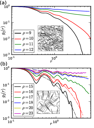
Upon increasing density, both zig-zag and bow-shaped molecules form a quasi-nematic phase with quasi-long-range orientational order . The quasi-nematic phase and the isotropic–quasi-nematic phase transition via disclination unbinding are evidenced by the transition from an exponential decay of at low to a power-law decay, , as increases (see Fig. 5). As per the discussion in Sec. III, the quasi-nematic phase is expected to be stable against spontaneous disclination unbinding when . We obtain the Frank elastic constants from the relation , where the power-law decay of is obtained from a linear fit of versus over the range . Note that the lower threshold is necessary because deviates from the power law at small , while the higher threshold is chosen so as to exclude correlations resulting from the use of periodic boundary conditions. Note also that bow-shaped molecules display correlation functions with fairly large oscillations as a result of the local packing structures, which do not exist for straight needles [see inset in Fig. 5(b)].

The results for the reduced Frank elastic constant are plotted in Fig. 6 for both molecule types. Since the results scale nearly linearly with , we identify the isotropic–quasi-nematic transition densities as the intersection between linear fits to data the points and [22].
For zig-zag molecules, the quasi-nematic phase is systematically destabilized by bending the terminal segments [Fig. 6(a)]. As the central- to-tail angle increases, the transition is thus pushed to higher densities. Bow-shaped molecules, however, show a non-monotonic trend of the transition density with [Fig. 6(b)]. For small the transition density increases with , while for the trend is inverted. In the range the quasi-nematic phase is unstable with respect to the modulated-nematic phase, and the power-law scaling analysis is then inapplicable (see Secs. IV.3 and IV.4).
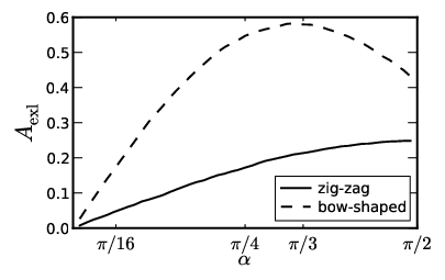
We try to understand the difference in the two molecular geometries by examining the size of the excluded area for perfectly parallel molecules (see Fig. 7). Like , it monotonically increases with for zig-zag molecules, but reaches a maximum at and then decreases for bow-shaped molecules. Large values of suggest that parallel molecules have to pack locally to come close to one another, as evidenced by the undulations of in Fig. 5(b). This packing constraints translational freedom, and thus reduces the translational contribution to the entropy. Because the translational contribution normally compensates for the loss of orientational freedom in the nematic phase, higher than usual are needed for this effect to be significant, and as a result increases.
IV.2 Quasi-nematic–smectic transition
Smectic order consists of a periodic arrangement of particle positions along one direction, which leads to a well-defined density wave along the corresponding wave vector. Within smectic layers, however, translational order is absent. Although long-range translational order is not expected in the thermodynamic limit of two-dimensional systems, smectic order is obervable on sufficiently small length scales. We get back to this point below. For now, we consider the smectic order parameter defined in Eq. (3) as a function of density for both the zig-zag and bow-shaped molecules in Fig. 8. The Monte Carlo simulation data are fitted with
| (14) |
where and are fit parameters. Hence, the quasi-nematic–smectic transition density is defined as the point of maximum slope of . The smectic order parameter for bow-shaped molecules does not assume large values even at the highest densities simulated, which is likely the result of out-of-layer fluctuations and of the instability of two-dimensional smectic order described. Fits to the simulation results nonetheless provide an estimate for . Note that the values of the transition densities identified in this way are close to the highest values of the densities explored in our simulation.

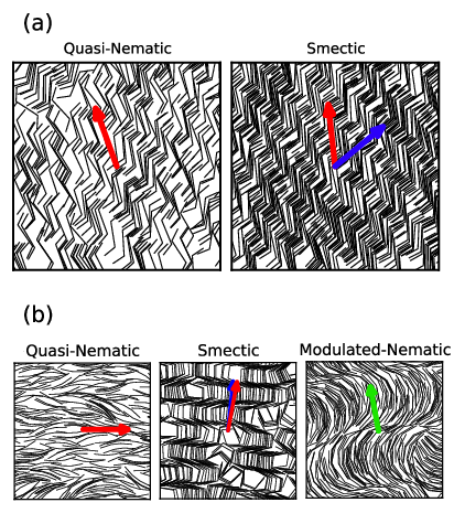
As could be seen in Fig. 2 and was previously noted in Ref. 48, zig-zag molecules form a smectic-C phase, wherein the nematic director is tilted with respect to the layer normal. Bow-shaped molecules instead arrange in an anti-ferromorphic smectic-A structure, wherein the polar vector adopts an opposite orientation in adjacent layers. This unusual ordering can be rationalized by extending a packing argument developed for the anti-ferrolectric ordering of V-shaped molecules[47], i.e., for [46]. Because the excluded area of two molecules is smaller in the anti-parallel () than in the parallel () arrangement, the former is entropically favored. Molecules can also more easily penetrate into neighboring layers in the anti-ferromorphic than in the ferromorphic smectic phase. This effect enhances out-of-layer fluctuations and thus entropically favors the anti-ferromorphic smectic ordering as well. This behavior is similar to that of three-dimensional bent-core molecules[73].
No significant smectic ordering is found for values of smaller than those given in Figs. 8(a) and (b). For zig-zag molecules at even smaller , we extrapolate the quasi-nematic–smectic transition to take place at that are inaccessible within a reasonable computational time; for bow-shaped molecules, however, the existence of a smectic phase at , even for large , is unclear.
As mentioned above and discussed in detail by Toner and Nelson in Ref. 74, two-dimensional long-range smectic order should not be thermodynamically stable. One expects instead the following scenario. At a given translational order is only disturbed by phonon fluctuations in regions with linear dimension smaller than a characteristic length , which is the mean distance between thermally induced dislocations. These dislocations thus destroy translational order on length scales larger than , but correlations in the layer orientations persist and exhibit a long-range algebraic decay. Although this scenario is physically reasonable and may explain the weak smectic ordering of bow-shaped molecules, we were unable to test it against our simulation data because of the limited range of computationally accessible . Instead, we find smectic order to be fully stabilized in our simulations.
IV.3 Modulated-nematic phase

Although at small and for bow-shaped molecules form a quasi-nematic phase [Fig. 2(b)], for intermediate , they also equilibrate in a modulated-nematic phase. In this phase no overall orientational or positional order exists [Fig. 9(a)]. Instead, it shows a different kind of supramolecular arrangement, wherein the orientation of a series of molecules varies gradually along arches that form approximate half-circles, and these arches themselves form layers. Periodic order exists along the layer normal but the mean polar vector in one layer is antiparallel to that of a neighboring layer. This arrangement destabilizes the quasi-nematic phase and its algebraic orientational order. As shown in Fig. 9(b), the occurrence of the modulated-nematic phase can even result in a reentrant exponential decay of with increasing . For , however, we found no evidence for a power-law decay of in the whole range of explored densities and a direct transition from the isotropic to modulated-nematic phase occurs.

In Fig. 10(a) the modulated-nematic order parameter defined in Eq. (5) is shown as a function of density for several values of . In analogy with the treatment for the identification of smectic order in Sec. IV.2, we fit (as obtained from the Monte Carlo simulation data) with a trial function similar to Eq. (14),
| (15) |
where and are fit parameters. In order to clarify the structural properties of the modulated-nematic phase, we consider the polar correlation function as defined in Eq. (6). Because of the periodic modulation in the molecular polar vector along the layer normal, becomes a periodic function when the layered structure is well established. In particular, since molecules in adjacent layers have opposite polarization, shows a minimum at a distance corresponding to the layer thickness followed by a maximum, which results from correlations with the next-nearest-neighbor layer. In Fig. 10(b) we show for and several values of . As expected, the periodic modulation of becomes stronger with increasing density indicating the progressive development of layers. This behavior is also observed for all other values of .

Our Monte Carlo data show that modulations in are already present at relatively small , whereas the order parameter has not yet increased much. For instance, for it can be seen in Fig. 10(b) that is already weakly modulated at , while the corresponding order parameter is only . Similarly, we find for the configuration shown in Fig. 9(a), even though a remarkable degree of layering is already clearly established. In other words, the layered structure of the modulated-nematic phase is established continuously, which makes it difficult to clearly establish a transition density. For this reason, we approximate the transition density into the modulated-nematic phase by using the threshold on the order parameter. The same threshold is used for all . This particular value is chosen in such a way that matches reasonably well the values of the density at which we observe the reentrant exponential decay of at .
The maximization procedure illustrated in Fig. 3(b) for determining the order parameter also provides the typical distance between two layers in the modulated-nematic phase, i.e., defined in Eq. (5). In Fig. 11 we show how this distance evolves with and compare it with the projected length of the molecule along the direction parallel to the central molecular segment, . At small , , which captures the supra-molecular structure of the modulated nematic phase. As increases, however, decreases, and it becomes comparable to at , indicating that molecules locally arrange in anti-ferromorphic order, as demonstrated by the inset (2) of Fig. 11, which is then favored over the supra-molecular ordering of the modulated-nematic phase. For the layering distance becomes smaller than , indicating that adjacent anti-ferromorphic layers on average slightly inter-penetrate, as discussed in Sec. IV.2.
The occurrence of a three-dimensional, spontaneously formed, modulated-nematic phase for banana-shaped mesogens and of the two-dimensional modulated-nematic phase for bow-shaped molecules, likely results from “pathological elasticity” [39], which has been predicted to be a consequence of the molecular curvature radius. In the standard Frank elastic theory, splay, bend, and twist elastic constants are indeed assumed to be positive in order to ensure a ground state with uniform nematic order. A non-uniform nematic ground state can thus be explained as resulting from a negative elastic constant, e.g., the bend constant, which is not forbidden by symmetry. Fourth-order terms in the elastic free energy are then needed to stabilize the modulated phase [39]. Our results thus indicate that there is an upper limit for the molecular curvature, corresponding in our model to , beyond which the supra-molecular structure of the modulated-nematic phase becomes unstable in favor of the anti-ferromorphic arrangement.
We already discussed in Sect. IV.2 that long-range order in two-dimensional smectics is not stable. In Fig. 9(b) in the center a dislocation in the layering of the supramolecular arches is visible. This might be an indication how, in analogy to two-dimensional smectics, also the layered structure is destabilized by the proliferation of dislocations in sufficiently large systems.
IV.4 Phase diagrams

In Fig. 12 we show the simulated phase diagrams for both the zig-zag and the bow-shaped molecules obtained using the approaches described in Secs. IV.1, IV.2, and IV.3. The dashed red and dotted blue lines show the predictions from Onsager theory for the transition densities and , respectively. We will review Onsager theory in Sec. V.
According to the phase diagram in Fig. 12(a), terminal segments of zig-zag particles destabilize the quasi-nematic phase but stabilize the smectic phase. This qualitative trend is captured by Onsager theory. Our simulation results are in rough agreement with previous studies[57, 48] but also exhibit some significant discrepancies. In particular, in our phase diagram both the isotropic–quasi-nematic and the quasi-nematic–smectic transitions appear at higher (Fig. 12(a)). In addition, for , the isotropic and smectic phases are well separated by the quasi-nematic phase, while the latter was not observed at all in previous studies. Most likely, the lower transition densities reported in Refs. 57, 48 follow from using the nematic order parameter for detecting the isotropic–quasi-nematic transition and from considering relatively small system sizes. As already mentioned, the nematic order parameter in a quasi-nematic phase decreases with system size [55].
Bow-shaped molecules exhibit a remarkably rich
behavior.
(1) For small , the low-density behavior is similar to that of zig-zag molecules.
The transition density (red circles) increases with increasing and is
underestimated by Onsager theory. Quasi-nematic order in this small- region is also
destabilized by further increasing the packing density. Instead of the emergence of a smectic phase, however, a
modulated-nematic phase takes precedence. We did not specifically explore the phase behavior of bow-shaped
molecules with , but we expect the modulated-nematic phase to appear at ever higher densities as
decreases, as indicated by the
dotted green line. For symmetry reasons the bent-nematic phase
cannot exist for .
(2) For
,
both the quasi-nematic and the
smectic orders are destabilized by
the modulated-nematic phase at all explored. The direct isotropic–modulated-nematic transition appears at increasing densities with . This phase is simply not captured by
Onsager theory as formulated in Sect. V.
(3) For , which is indicated in the phase diagram as a gray area, we find no clear evidence for any of the mesophases known to be formed by bow-shaped molecules. In this region
the distance between two adjacent layers approaches the projection of the total molecular length along the molecular central segment, resulting in a strong competition between the formation of supra-molecular layers and anti-ferromorphic domains. The investigation of configurations at densities much higher than the ones we could reach would be necessary to clarify what mesophase, if any, is stable in that system.
(4) For , the molecular curvature is too large to induce
a spontaneous bending of the nematic director and the corresponding layer formation.
Quasi-nematic order then becomes stable again, but this time the transition densities
decrease with increasing .
The isotropic–quasi-nematic transition is highly overestimated by Onsager theory.
The theory strongly relies on the excluded area, as discussed in Sec. II.5, but
the excluded area of bow-shaped molecules is minimal in the anti-parallel configuration. In our simulations
we instead observe clusters of molecules packed in parallel.
Because this arrangement involves structural correlations between more than two molecules, it is not surprising that Onsager theory, which only takes into account two-particle correlations dramatically fails.
Note that we did not study molecules with . With this central-to-tail angle parallel molecules cannot anymore be shifted into each other to form closely packed clusters. A different phase is thus expected. Tetradic order has indeed been observed in related models[45].
V Onsager Theory for Phase Diagrams
In Ref. 57, a density functional theory in mean-field approximation was used to determine the phase behavior of zig-zag molecules. Based on the second-order virial expansion of the free energy introduced by Onsager, predictions for both and were made [57]. In the following, we summarize and extend the results of this Onsager theory.
We start with the free energy functional
| (16) | |||||
where is the local number density in terms of particle position and particle orientation . The Mayer function of the pair potential is simple for hard-core particles. It is zero except when particles overlap, where .
In the isotropic and nematic phases, positional order does not exist and one has . In the second term of the Onsager free energy functional (16), this introduces the excluded area in terms of the angle between the two molecular orientations in two dimensions. Expanding orientational distribution and into Fourier modes and minimizing with respect to the Fourier amplitudes of , gives a series of possible bifurcation densities
| (17) |
Here, is the -th Fourier amplitude of the excluded area ,
| (18) |
We have introduced an index for zig-zag molecules and for bow-shaped molecules because their respective excluded areas either have a period or . We determine the Fourier coefficients numerically by means of the Monte Carlo integration technique described in Sec. II.5. We choose the lowest positive value of as the transition density , which is realized at for zig-zag molecules and at for bow-shaped molecules. The resulting transition lines are plotted as red dashed lines in the phase diagrams of Fig. 12.
To determine the nematic–smectic transition density , we choose a periodic modulation for the density along the axis, , and assume perfect alignment of the molecules as in Ref. 57, because the nematic order in the smectic phase is typically very high. The evaluation of the free energy functional now involves an excluded distance , where is the orientation angle of the central molecular segment with respect to the smectic layer normal. The excluded distance is related to the excluded area by . Taking into account only the first Fourier mode of the density modulation in the free energy and minimizing with respect to the Fourier amplitude, we obtain an equation for the nematic–smectic transition density ,
| (19) |
where is the smectic period. The tilt angle and the period are also determined by minimizing the free energy functional. For details of the calculation, we refer the reader to the work of Varga et al.[57]. Note that we were only able to calculate a nematic–smectic transition line for zig-zag molecules. It is plotted in the phase diagram of Fig. 12 (a) as blue dotted line.
As already discussed, for the zig-zag molecules Onsager theory qualitatively captures the behavior of both the isotropic–nematic and the nematic–smectic transition lines. Both lines are underestimated by the theory, but that is hardly surprising. Onsager theory relies on a second-order virial expansion of the system’s free energy, which is strictly valid only in the dilute regime, while in our model orientational and translational order occur at relatively high densities. Indeed, it was shown that virial coefficients of order higher than two are not negligible in hard-needle systems [54]. In addition, Onsager theory does not take into account topological defects that play a significant role in the two-dimensional phase behavior and phase transitions. In Ref. 57 good agreement between predictions from Onsager theory and results from Monte Carlo simulations are reported for zig-zag molecules. We believe this agreement to be due in part to the small system size of 200 molecules, where defects cannot fully develop.
VI Conclusion
Despite its simplicity, the bent-needle model discussed in this paper shows a variety of liquid-crystal phases and gives an example of how molecular geometry controls their formation.
Chiral zig-zag molecules assume quasi-nematic and smectic phases, depending on density and the central-to-tail angle . We use the orientational correlation function , which decays exponentially in the isotropic phase and algebraically in the orientationally ordered phase, to identify the isotropic–quasi-nematic transition. In two-dimensional systems with short-ranged interactions, one expects the transition to take place via disclination unbinding [70]. Indeed, apart from packing effects, the correlation functions described in Sec. IV.1 behave similarly to the ones already reported in other two-dimensional anisotropic models with hard-core interactions [22, 54, 55, 56]. For the zig-zag molecule the isotropic–nematic transition density increases with increasing central-to-tail angle , while the nematic–smectic transition, , exhibits the opposite trend. Such behavior is qualitatively captured by Onsager theory although both and are underestimated by the theory, as discussed in Sec. V.
Furthermore, we observe a smectic C phase, where the central segment of the zig-zag molecule is tilted against the layer normal. The clear formation of smectic layers, however, indicates that our systems are too small to observe the dislocation unbinding scenario predicted in Ref. 74.
Achiral bow-shaped molecules have a much richer phase behavior. It can be divided into three regions, depending on the value of . For small molecules form isotropic, quasi-nematic, and modulated-nematic phases, as density increases. The isotropic–quasi-nematic transition is defect driven, which makes the orientational correlation function switch from an exponential to power-law decay with increasing density. No polar order is found in the quasi-nematic phase. Further increasing density destabilizes the orientational order of the quasi-nematic phase. A modulated-nematic phase then takes over, wherein bow-shaped molecules form layers of supramolecular arches. The orientational correlation function shows a reentrant exponential decay that corresponds to the development of the supramolecular arches. At intermediate , a direct transition from the isotropic to the modulated-nematic phase takes place. The modulated-nematic structure becomes less pronounced with increasing , i.e., the layer thickness decreases towards the molecule length, up to the point where the formation of supramolecular arches becomes unfavored and anti-ferromorphic domains develop instead. For , the curvature radius of the molecules becomes too small to induce spontaneous bending of the nematic director and quasi-nematic order reenters. Anti-ferromorphic smectic order is then found at even higher density.
A very appealing result of our investigation is the identification of the modulated-nematic phase made from supramolecular layers, which strongly depend on molecular geometry. Our simulations are the first to clearly demonstrate such a layered structure in two dimensions and to relate it to molecular geometry. We find the optimal value of the curvature radius to be around when the modulated-nematic phase occurs at the lowest packing density. This finding might be particularly useful in developing novel functional optical materials based on organic bent-core liquid crystals[75, 76], where the formation of polar domains can be used to tune the nonlinear optical properties of the material.
Our investigations further illustrate the richness of structures, including supra-molecular organization, formed by self-assembling particles of different shapes. Being able to control molecular geometry thus offers the possibility of designing novel materials, in particular in two dimensions, and of tuning their properties accordingly.
Acknowledgements.
This work was supported by the Deutsche Forschungsgemeinschaft through the international research training group IRTG 1524. PC is thankful for support from the National Science Foundation Research Triangle Materials Research Science and Engineering Center (DMR-1121107).References
- [1] A. Ulman, An Introduction to Ultrathin Organic Films: From Langmuir–Blodgett to Self–Assembly (Academic press, 2013).
- [2] F. Schreiber, J. of Phys. Condens. Matter 16, R881 (2004).
- [3] A. Böker, J. He, T. Emrick, and T. P. Russell, Soft Matter 3, 1231 (2007).
- [4] J. V. Barth, G. Costantini, and K. Kern, Nature 437, 671 (2005).
- [5] D. Aswal, S. Lenfant, D. Guerin, J. Yakhmi, and D. Vuillaume, Anal. Chim. Acta 568, 84 (2006).
- [6] J. Hicks and T. Petralli-Mallow, Appl. Phys. B 68, 589 (1999).
- [7] P. M. Mendes, Chem. Soc. Rev. 37, 2512 (2008).
- [8] M. J. Hore and R. J. Composto, ACS nano 4, 6941 (2010).
- [9] R. S. Mclean, X. Huang, C. Khripin, A. Jagota, and M. Zheng, Nano Lett. 6, 55 (2006).
- [10] K. Slyusarenko, D. Constantin, and P. Davidson, J. Chem. Phys. 140, 104904 (2014).
- [11] V. Fournée, É. Gaudry, J. Ledieu, M.-C. De Weerd, D. Wu, and T. Lograsso, ACS nano 8, 3646 (2014).
- [12] J. Mikhael, M. Schmiedeberg, S. Rausch, J. Roth, H. Stark, and C. Bechinger, Proc. Natl. Acad. Sci. U.S.A. 107, 7214 (2010).
- [13] M. Schmiedeberg and H. Stark, Phys. Rev. Lett. 101, 218302 (2008).
- [14] M. Schmiedeberg, J. Mikhael, S. Rausch, J. Roth, L. Helden, C. Bechinger, and H. Stark, Eur. Phys. J. E 32, 25 (2010).
- [15] Y. He, Y. Chen, H. Liu, A. E. Ribbe, and C. Mao, J. Am. Chem. Soc. 127, 12202 (2005).
- [16] E. Winfree, F. Liu, L. A. Wenzler, and N. C. Seeman, Nature 394, 539 (1998).
- [17] Y. Bai and N. L. Abbott, Langmuir 27, 5719 (2010).
- [18] W. H. de Jeu, B. I. Ostrovskii, and A. N. Shalaginov, Rev. Mod. Phys. 75, 181 (2003).
- [19] I. Muševič, M. Škarabot, U. Tkalec, M. Ravnik, and S. Žumer, Science 313, 954 (2006).
- [20] A. Mulero, Theory and simulation of hard-sphere fluids and related systems, Vol. 753 (Springer Science & Business Media, 2008).
- [21] A. Haji-Akbari, M. Engel, A. S. Keys, X. Zheng, R. G. Petschek, P. Palffy-Muhoray, and S. C. Glotzer, Nature 462, 773 (2009).
- [22] M. Bates and D. Frenkel, J. Chem. Phys. 112, 10034 (2000).
- [23] A. Ghosh and D. Dhar, EPL 78, 20003 (2007).
- [24] P. Kählitz and H. Stark, J. Chem. Phys. 136, 174705 (2012).
- [25] A. Donev, J. Burton, F. H. Stillinger, and S. Torquato, Phys. Rev. B 73, 054109 (2006).
- [26] Y. Martínez-Ratón, E. Velasco, and L. Mederos, J. Chem. Phys. 122, 064903 (2005).
- [27] M. C. Lagomarsino, M. Dogterom, and M. Dijkstra, J. Chem. Phys. 119, 3535 (2003).
- [28] P. Kählitz, M. Schoen, and H. Stark, J. Chem. Phys. 137, 224705 (2012).
- [29] W.-S. Xu, Y.-W. Li, Z.-Y. Sun, and L.-J. An, J. Chem. Phys. 139, 024501 (2013).
- [30] M. Moradi, S. Hashemi, and F. Taghizadeh, Physica A 389, 4510 (2010).
- [31] C. Care and D. Cleaver, Rep. Prog. Phys. 68, 2665 (2005).
- [32] T. C. Lubensky, Phys. Rev. E 66, 031704 (2002).
- [33] H. Takezoe and Y. Takanishi, Jpn. J. Appl. Phys. 45, 597 (2006).
- [34] G. Pelzl, S. Diele, and W. Weissflog, Adv. Mater. , 707 (1999).
- [35] M. B. Ros, J. L. Serrano, M. R. de la Fuente, and C. L. Folcia, J. Mater. Chem. 15, 5093 (2005).
- [36] R. Berardi, L. Muccioli, S. Orlandi, M. Ricci, and C. Zannoni, J. Phys. Cond. Matt. 20, 463101 (2008).
- [37] P. I. C. Teixeira, J. Masters, and B. M. Mulder, Mol. Cryst. Liq. Cryst. 323, 167 (1998).
- [38] G. Pelzl, A. Eremin, S. Diele, H. Kresse, and W. Weissflog, J. Mater. Chem. 12, 2591 (2002).
- [39] I. Dozov, EPL 247 (2001).
- [40] P. J. Camp, M. P. Allen, and A. J. Masters, J. Chem. Phys. 111, 9871 (1999).
- [41] S. J. Johnston, R. J. Low, and M. P. Neal, Phys. Rev. E 65, 051706 (2002).
- [42] A. Dewar and P. J. Camp, Phys. Rev. E 70, 011704 (2004).
- [43] S. M. Shamid, S. Dhakal, and J. V. Selinger, Phys. Rev. E 87, 052503 (2013).
- [44] P. Grzybowski and L. Longa, Phys. Rev. Lett. 107, 027802 (2011).
- [45] J. Martínez-González, J. C. Armas-Pérez, and J. Quintana-H, J. Stat. Phys. 150, 559 (2012).
- [46] F. Bisi, R. Rosso, E. Virga, and G. Durand, Phys. Rev. E 78, 011705 (2008).
- [47] J. Martínez-González, S. Varga, P. Gurin, and J. Quintana-H., EPL 97, 26004 (2012).
- [48] J. Peón, J. Saucedo-Zugazagoitia, F. Pucheta-Mendez, R. A. Perusquía, G. Sutmann, and J. Quintana-H, J. Chem. Phys. 125, 104908 (2006).
- [49] N. D. Mermin, Phys. Rev. 176, 250 (1968).
- [50] K. J. Strandburg, Rev. Mod. Phys. 60, 161 (1988).
- [51] E. P. Bernard and W. Krauth, Phys. Rev. Lett. 107, 155704 (2011).
- [52] V. Borshch, Y.-K. Kim, J. Xiang, M. Gao, A. Jákli, V. P. Panov, J. K. Vij, C. T. Imrie, M.-G. Tamba, G. H. Mehl, et al., Nat. commun. 4 (2013).
- [53] R. Memmer, Liq. Cryst. 29, 483 (2002).
- [54] D. Frenkel and R. Eppenga, Phys. Rev. A (1985).
- [55] R. L. Vink, Eur. Phys. J. B 72, 225 (2009).
- [56] J. C. Armas-Pérez and J. Quintana-H., Phys. Rev. E 83, 051709 (2011).
- [57] S. Varga, P. Gurin, J. C. Armas-Pérez, and J. Quintana-H, J. Chem. Phys. 131, 184901 (2009).
- [58] R. A. Perusquı́a, J. Peón, and J. Quintana, Physica A 345, 130 (2005).
- [59] J. Polson and D. Frenkel, Phys. Rev. E 56, R6260 (1997).
- [60] D. Frenkel and B. Smit, “Understanding Molecular Simulation: From Algorithms to Applications,” (1997).
- [61] M. Miller, L. Amon, and W. Reinhardt, Chem. Phys. Lett. 331, 278 (2000).
- [62] G. Sutmann and V. Stegailov, J. Mol. Liq. 125, 197 (2006).
- [63] J. Wang and R. Swendsen, Physica A 167, 565 (1990).
- [64] C. Dressts and W. Krauth, J. Phys. A-Math. Gen. 28, L597 (1995).
- [65] S. Whitelam and P. L. Geissler, J. Chem. Phys. 127, 154101 (2007).
- [66] D. Wu, D. Chandler, and B. Smitt, J. Phys. Chem. 96, 4077 (1992).
- [67] L. Onsager, Ann. N. Y. Acad. Sci. (1949).
- [68] Y. Martínez-Ratón, E. Velasco, and L. Mederos, J. Chem. Phys. 122, 064903 (2005).
- [69] N. Mermin and H. Wagner, Phys. Rev. Lett. 17, 1133 (1966).
- [70] J. Kosterlitz and D. Thouless, J. Phys. C Solid State 1181 (1973).
- [71] D. R. Nelson and R. A. Pelcovits, Phys. Rev. B 16, 2191 (1977).
- [72] P. M. Chaikin and T. C. Lubensky, Principles of condensed matter physics, Vol. 1 (Cambridge Univ Press, 2000).
- [73] Y. Lansac, P. K. Maiti, N. A. Clark, and M. A. Glaser, Phys. Rev. E 67, 011703 (2003).
- [74] J. Toner and D. Nelson, Phys. Rev. B 23, 316 (1981).
- [75] J. Etxebarria and M. B. Ros, J. Mater. Chem. 18, 2919 (2008).
- [76] I. C. Pintre, J. L. Serrano, M. B. Ros, J. Martínez-Perdiguero, I. Alonso, J. Ortega, C. L. Folcia, J. Etxebarria, R. Alicante, and B. Villacampa, J. Mater. Chem. 20, 2965 (2010).