跳到论文正文
W Papers独立论文阅读器 arXiv:1506.02470 论文正文 计算阅读时间 · 0%
引用这篇论文根据当前论文元数据生成,正式投稿前建议核对。


License: arXiv.org perpetual non-exclusive license
arXiv:1506.02470v2 [math.AP] 09 Sep 2015
††footnotetext: This research was partially supported by the FWF-doctoral school “Dissipation and dispersion in nonlinear partial differential equations” and INDAM - GNFM from Italy. One author (AA) is grateful to J. Schöberl for very helpful discussions.

Large-time behavior in non-symmetric Fokker-Planck equations

Franz Achleitner Address: Institute for Analysis and Scientific Computing, Technical University Vienna, Wiedner Hauptstraße 8, A-1040 Vienna Email: franz.achleitner@tuwien.ac.at , Anton Arnold Address: Institute for Analysis and Scientific Computing, Technical University Vienna, Wiedner Hauptstraße 8, A-1040 Vienna Email: anton.arnold@tuwien.ac.at and Dominik Stürzer Address: Institute for Analysis and Scientific Computing, Technical University Vienna, Wiedner Hauptstraße 8, A-1040 Vienna Email: dominik.stuerzer@tuwien.ac.at
Abstract

We consider three classes of linear non-symmetric Fokker-Planck equations having a unique steady state and establish exponential convergence of solutions towards the steady state with explicit (estimates of) decay rates. First, “hypocoercive” Fokker-Planck equations are degenerate parabolic equations such that the entropy method to study large-time behavior of solutions has to be modified. We review a recent modified entropy method (for non-symmetric Fokker-Planck equations with drift terms that are linear in the position variable). Second, kinetic Fokker-Planck equations with non-quadratic potentials are another example of non-symmetric Fokker-Planck equations. Their drift term is nonlinear in the position variable. In case of potentials with bounded second-order derivatives, the modified entropy method allows to prove exponential convergence of solutions to the steady state. In this application of the modified entropy method symmetric positive definite matrices solving a matrix inequality are needed. We determine all such matrices achieving the optimal decay rate in the modified entropy method. In this way we prove the optimality of previous results. Third, we discuss the spectral properties of Fokker-Planck operators perturbed with convolution operators. For the corresponding Fokker-Planck equation we show existence and uniqueness of a stationary solution. Then, exponential convergence of all solutions towards the stationary solution is proven with an uniform rate.

Key words and phrases: 
Fokker-Planck equation, hypocoercivity, entropy method, large-time behavior, spectral gap, sharp decay rate, non-local perturbation, spectral analysis, exponential stability.
2010 Mathematics Subject Classification
Primary 35Q84, 35H10, 35B20; Secondary 35K10, 35B40, 47D07, 35P99, 47D06

1. Introduction

Fokker-Planck equations (FPEs) describe the deterministic evolution of the probability density associated to many stochastic processes [35]. Hence, they constitute an important class of models in applied mathematics and an interesting object of study in the analysis of PDEs. This paper is concerned with the large time analysis of FPEs. In particular we shall analyze non-symmetric equations (corresponding to irreversible stochastic processes). We shall analyze the existence of unique (normalized) steady states and, in particular, the convergence of the time dependent solutions towards it. Here, the main emphasis will be put on the derivation of explicit exponential decay rates (or, at least, estimates of it). Apart from an intrinsic mathematical interest in such decay rates, they are even relevant for the modeling of industrial processes, like the fiber lay-down processes in technical textile production (cf. [27]).

For linear, symmetric FPEs the sharp exponential decay rate equals the spectral gap of the generator of the evolution. But, apart from simple examples, exact values or good estimates of this spectral gap are rarely available. Based on the work of Bakry and Émery on diffusion processes [9, 10], the entropy method for PDEs has become an important tool to study the large time behavior of wide classes of parabolic equations [7, 2, 3]. The success of this approach is mainly due to its robustness to nonlinear perturbations and extensions [16, 14]. More recently it was even generalized to degenerate parabolic equations [41, 17, 5].

In this paper we shall focus on the large-time behavior of three classes of linear, non-symmetric FPEs: In §2 we shall consider non-symmetric FPEs with drift terms that are linear in the position variable. The recent interest in these equations originated actually in developing entropy methods for the subclass of degenerate diffusions equations, or more precisely “hypocoercive” equations. But it turned out that this method can be viewed more naturally for non-symmetric FPEs. The material of this chapter will be based on the recently developed entropy method from [5]. We shall present a review from an updated point of view and include several typical examples to illustrate this new method.

In §3 we shall analyze kinetic FPEs with non-quadratic potentials. Again, they are non-symmetric FPEs, but with a drift term that is nonlinear in the position variable. This will illustrate that the entropy method from §2 can be applied also beyond equations with linear drift, at least in perturbative settings. The material of this chapter is an improvement of §7 in [5].

§4 will be concerned with FPEs with non-local perturbations. These perturbations will again render the evolution generator non-symmetric in an appropriately weighted L2L^{2}–space. But, surprisingly, a wide class of non-local perturbations does not modify the spectrum of the underlying (standard symmetric) FPE. Hence, we shall use spectral methods for the large-time analysis of such models. The material of this chapter is an extension of [37] to FPEs with diffusion and drift matrices that are not the identity.

2. Hypocoercive and non-symmetric Fokker-Planck equations

In this chapter we shall study the evolution of a function f⁡(t,x);f(t,x); t≥0,x∈ℝdt\geq 0,\,x\in\mathbb{R}^{d}, under the linear FPE of the form

(2.1) ∂tf\displaystyle\partial_{t}f =Lf:=div(𝐃∇f+𝐂xf),\displaystyle=Lf:=\operatorname{div}({\mathbf{D}}\nabla f+\mathbf{C}x\ f)\,,

and subject to the initial condition f⁡(t=0)=f0f(t=0)=f_{0}. Without restriction of generality we assume that

f0≥0,∫ℝdf0​d⁡x=1.f_{0}\geq 0\,,\quad\int_{\mathbb{R}^{d}}f_{0}\,\operatorname{d}\!x=1\,.

We stipulate that solutions satisfy f⁡(t,⋅)∈L1​(ℝd)f(t,\cdot)\in L^{1}(\mathbb{R}^{d}). Hence, the divergence form of (2.1) implies ∫ℝdf⁡(t,x)​d⁡x=1\int_{\mathbb{R}^{d}}f(t,x)\,\operatorname{d}\!x=1 for all t>0t>0. In (2.1), the diffusion matrix 𝐃∈ℝd×d{\mathbf{D}}\in\mathbb{R}^{d\times d} is symmetric and positive semi-definite, and 𝐂∈ℝd×d\mathbf{C}\in\mathbb{R}^{d\times d} is the drift matrix. Both are constant in space and time.

An important model of this class is the kinetic FPE from plasma physics [35, 40]. The time evolution of the phase space probability density f⁡(t,x,v)f(t,x,v) is governed by:

(2.2) ∂tf+v⋅∇xf−∇xV⋅∇vf\displaystyle\partial_{t}f+v\cdot\nabla_{x}f-\nabla_{x}V\cdot\nabla_{v}f =ν​divv⁡(v​f)+σ​Δv​f;x,v∈ℝn;t>0.\displaystyle=\nu\operatorname{div}_{v}(vf)+\sigma\Delta_{v}f\,;\quad x,\,v\in\mathbb{R}^{n};\,t>0\,.

Here, the position-velocity vector (x,v)(x,v) plays the role of x∈ℝd,d=2​nx\in\mathbb{R}^{d},\,d=2n, in (2.1). ν,σ\nu,\sigma denote (positive) friction and diffusion parameters, respectively. V=V⁡(x)V=V(x) is a given confinement potential for the system. Next we rewrite (2.2) as

ft\displaystyle f_{t} =\displaystyle= divx,v⁡[(𝟎𝟎𝟎σ​𝐈)​∇x,vf+(−v∇xV+ν​v)].\displaystyle\operatorname{div}_{x,v}\left[\left(\begin{array}[]{cc}\mathbf{0}&\mathbf{0}\\ \mathbf{0}&\sigma\,\mathbf{I}\end{array}\right)\nabla_{x,v}f+\left(\begin{array}[]{c}-v\\ \nabla_{x}V+\nu\,v\end{array}\right)\,\right]\,.

Here, the first matrix is a singular diffusion matrix, with the identity matrix 𝐈∈ℝn×n\mathbf{I}\in\mathbb{R}^{n\times n}; the second term is the drift. For a quadratic potential VV, the kinetic FPE (2.2) takes exactly the form of (2.1) and its analysis will be covered in §2. The case of non-quadratic potentials is the subject of §3.

The goal of this chapter is first to identify (under appropriate assumptions on 𝐃{\mathbf{D}} and 𝐂\mathbf{C}) the unique normalized steady state f∞​(x)f_{\infty}(x) of (2.1). Most of all, we shall then study the convergence of f⁡(t)f(t) to f∞f_{\infty} as t→∞t\to\infty with (possibly sharp) exponential rates. In view of space limitations we shall mostly present only formal computations, which hold rigorously for regular enough solutions. But, anyhow, parabolic and hypocoercive FPEs regularize instantaneously to C∞C^{\infty} (cf. Proposition 2.6 below). So, regularity is actually not an issue, with the possible exemption at the initial time.

2.1. Non-symmetric Fokker-Planck equations

In this section we introduce the notion of (non)symmetric FPEs and the relative entropy, which will be our main tool to analyze the large-time behavior below. For these definitions we first consider FPEs with xx–dependent coefficients. A symmetric Fokker-Planck equation is defined to be of the form

(2.8) ∂tf=L1f:=div(𝐃(x)[∇f+f∇A(x)]),\partial_{t}f=L_{1}f:=\operatorname{div}\big({\mathbf{D}}(x)[\nabla f+f\nabla A(x)]\big),

with a diffusion matrix 𝐃{\mathbf{D}} that is locally uniformly positive definite on ℝd\mathbb{R}^{d} and symmetric. We assume that the sufficiently regular confinement potential AA satisfies e−A∈L1​(ℝd)\mathrm{e}^{-A}\in L^{1}(\mathbb{R}^{d}). Then f∞:=e−Af_{\infty}:=\mathrm{e}^{-A} is the unique normalized steady state of (2.8). The normalization ∫ℝdf∞​(x)​d⁡x=1\int_{\mathbb{R}^{d}}f_{\infty}(x)\,\operatorname{d}\!x=1 is imposed here by changing the additive constant of AA, which is not prescribed by (2.8). The non-degeneracy of the ground state of L1L_{1} can easily be seen from the following computation:

(2.9) ⟨L1f,g⟩H=−∫ℝd∇T(ff∞)𝐃(x)∇(gf∞)f∞dx,\langle L_{1}f,g\rangle_{H}=-\int_{\mathbb{R}^{d}}\nabla^{T}\big(\frac{f}{f_{\infty}}\big){\mathbf{D}}(x)\nabla\big(\frac{g}{f_{\infty}}\big)\ f_{\infty}\,\operatorname{d}\!x\,,

with ⟨⋅,⋅⟩H\langle\cdot,\cdot\rangle_{H} denoting the inner product in the weighted L2L^{2}–space H:=L2​(ℝd,f∞−1)H:=\linebreak L^{2}(\mathbb{R}^{d},f_{\infty}^{-1}). And the right hand side of (2.9), with f=gf=g, vanishes iff f/f∞=c​o​n​s​tf/f_{\infty}=const. The quadratic form (2.9) also shows that the operator L1L_{1} is symmetric in HH (cf. §2 of [7] for more details).

The key feature of a symmetric FPE is the gradient form of its drift vector field. For d≥2d\geq 2 we shall now consider more general drift fields, which will make the evolution generator non-symmetric in HH. For regular diffusion matrices 𝐃⁡(x){\mathbf{D}}(x), the following equation is called a non-symmetric Fokker-Planck equation:

(2.10) ∂tf=L2​f:=div⁡(𝐃⁡(x)​[∇f+f⁡{∇A​(x)+F⁡(x)}]).\partial_{t}f=L_{2}f:=\operatorname{div}\big({\mathbf{D}}(x)[\nabla f+f\{\nabla A(x)+F(x)\}]\big)\,.

Here we assume that the additional vector field FF satisfies

(2.11) div⁡(𝐃⁡(x)​F​(x)​f∞​(x))=0,∀x∈ℝd,\operatorname{div}({\mathbf{D}}(x)F(x)\ f_{\infty}(x))=0\,,\quad\forall\,x\in\mathbb{R}^{d}\,,

such that f∞=e−Af_{\infty}=\mathrm{e}^{-A} is still the unique steady state of (2.10).

In typical applications, however, the FPE is given with just one drift vector field that is not yet split into two summands (in contrast to (2.10)). In order to retrieve the steady state, this field then needs to be decomposed into a gradient part and a divergence free part (in the above sense). This task is a generalization of the Helmholtz-Hodge decomposition (see §2 in [4] for a typical example). Such a decomposition of the vector field readily yields the following decomposition of the operator L2L_{2} into its symmetric part LsL_{s} in HH and its anti-symmetric part La​sL_{as}: L2=Ls+La​sL_{2}=L_{s}+L_{as} with

Ls​f\displaystyle L_{s}f =div(𝐃(x)[∇f+f∇A(x)]),\displaystyle=\operatorname{div}\big({\mathbf{D}}(x)[\nabla f+f\nabla A(x)]\big)\,,
La​s​f\displaystyle L_{as}f =div⁡(𝐃⁡(x)​F​(x)​f).\displaystyle=\operatorname{div}\big({\mathbf{D}}(x)F(x)\ f\big)\,.

Due to (2.11) we have Ls​f∞=La​s​f∞=0L_{s}f_{\infty}=L_{as}f_{\infty}=0.

Next we give a more compact form of LsL_{s} and La​sL_{as}, which of course also holds for L1L_{1} with F≡0F\equiv 0.

Lemma 2.1.

Let 𝐃⁡(x)>𝟎{\mathbf{D}}(x)>\mathbf{0}, assume condition (2.11), and let f∞=e−Af_{\infty}=\mathrm{e}^{-A} denote the steady state of (2.10). The symmetric/anti-symmetric decomposition of L2L_{2} then satisfies:

(2.12) Ls​f\displaystyle L_{s}f\!\!\!\! =\displaystyle= div(f∞𝐃(x)∇ff∞),\displaystyle\!\!\!\!\operatorname{div}\Big(f_{\infty}\ {\mathbf{D}}(x)\nabla\frac{f}{f_{\infty}}\Big)\,,
(2.13) La​s​f\displaystyle L_{as}f\!\!\!\! =\displaystyle= div(f∞𝐑(x)∇ff∞),\displaystyle\!\!\!\!\operatorname{div}\Big(f_{\infty}\ \mathbf{R}(x)\nabla\frac{f}{f_{\infty}}\Big)\,,

where the matrices 𝐑⁡(x)∈ℝd×d\mathbf{R}(x)\in\mathbb{R}^{d\times d} are skew-symmetric and satisfy on ℝd\mathbb{R}^{d}:

(2.14) ∇T(𝐑​f∞)=GT:=(𝐃​F​f∞)T.\nabla^{T}(\mathbf{R}f_{\infty})=G^{T}:=({\mathbf{D}}F\ f_{\infty})^{T}\,.
Proof.

(2.12) is trivial, so we only discuss (2.13). The divergence-free-condition (2.11) on the vector field GG implies that there exists a matrix function 𝐁⁡(x)∈ℝd×d\mathbf{B}(x)\in\mathbb{R}^{d\times d}, with 𝐁⁡(x)\mathbf{B}(x) skew-symmetric and

(2.15) GT​(x)=∇T𝐁​(x).G^{T}(x)=\nabla^{T}\mathbf{B}(x)\,.

Let us briefly illustrate this statement: For d=2, 3d=2,\,3 (2.15) simplifies to the well known representations of divergence free vector fields:

𝐁⁡(x)=(0−b⁡(x)b⁡(x)0),G=∇⟂b,∇⟂:=(∂x2−∂x1),\mathbf{B}(x)=\left(\begin{array}[]{cc}0&-b(x)\\ b(x)&0\end{array}\right)\,,\qquad G=\nabla^{\perp}b\,,\qquad\nabla^{\perp}:=\left(\begin{array}[]{c}\partial_{x_{2}}\\ -\partial_{x_{1}}\end{array}\right)\,,

and, respectively,

𝐁⁡(x)=(0−b3​(x)b2​(x)b3​(x)0−b1​(x)−b2​(x)b1​(x)0),G=curl⁡(b1​(x)b2​(x)b3​(x)).\mathbf{B}(x)=\left(\begin{array}[]{ccc}0&-b_{3}(x)&b_{2}(x)\\ b_{3}(x)&0&-b_{1}(x)\\ -b_{2}(x)&b_{1}(x)&0\end{array}\right)\,,\qquad G=\operatorname{curl}\left(\begin{array}[]{c}b_{1}(x)\\ b_{2}(x)\\ b_{3}(x)\end{array}\right)\,.

In higher dimensions, (2.15) can be verified either with differential forms (cf. §6 in [8], [15]) or by Fourier transformation.

Next we compute

La​sf:=div(Gff∞)=div((∇T𝐁)Tff∞)=(∇T𝐁)∇ff∞=div(𝐁∇ff∞),L_{as}f:=\operatorname{div}\Big(G\,\frac{f}{f_{\infty}}\Big)=\operatorname{div}\Big((\nabla^{T}\mathbf{B})^{T}\frac{f}{f_{\infty}}\Big)=(\nabla^{T}\mathbf{B})\nabla\frac{f}{f_{\infty}}=\operatorname{div}\Big(\mathbf{B}\nabla\frac{f}{f_{\infty}}\Big)\,,

where we have used the skewness of 𝐁\mathbf{B} in the last two steps. Setting 𝐑:=𝐁​f∞−1\mathbf{R}:=\mathbf{B}f_{\infty}^{-1} yields (2.13). ∎

Note that La​sL_{as} in (2.13) is only a first order operator – due to the skew-symmetry of 𝐑⁡(x)\mathbf{R}(x).

As mentioned above, the main goal of this chapter is to study the convergence to the equilibrium for solutions to non-symmetric FPEs. To this end, our main tool will be the relative entropy. We define (see §2.2 of [7] for more details):

Definition 2.2.
  1. (a)

    Let JJ be either ℝ+\mathbb{R}^{+} or ℝ\mathbb{R}. A scalar function ψ∈C⁡(J¯)∩C4​(J)\psi\in C(\bar{J})\cap C^{4}(J) satisfying the conditions

    (2.16) ψ⁡(1)=0,ψ≥0,ψ′′>0,(ψ′′′)2≤12​ψ′′​ψI​V​ on ​J\psi(1)=0\,,\quad\psi\geq 0\,,\quad\psi^{\prime\prime}>0\,,\quad(\psi^{\prime\prime\prime})^{2}\leq\frac{1}{2}\psi^{\prime\prime}\psi^{IV}\;\mbox{ on }J

    is called entropy generator.

  2. (b)

    Let f1∈L1​(ℝd)f_{1}\in L^{1}(\mathbb{R}^{d}), f2∈L+1​(ℝd)f_{2}\in L^{1}_{+}(\mathbb{R}^{d}) with ∫ℝdf1​d⁡x=∫ℝdf2​d⁡x=1\int_{\mathbb{R}^{d}}f_{1}\,\operatorname{d}\!x=\int_{\mathbb{R}^{d}}f_{2}\,\operatorname{d}\!x=1 and f1f2​(x)∈J¯\frac{f_{1}}{f_{2}}(x)\in\bar{J} a.e. (w.r.t. the measure f2​(d⁡x)f_{2}(\,\operatorname{d}\!x)). Then

    (2.17) eψ​(f1|f2):=∫ℝdψ⁡(f1f2)​f2​d⁡x≥0e_{\psi}(f_{1}|f_{2}):=\int_{\mathbb{R}^{d}}\psi\Big(\frac{f_{1}}{f_{2}}\Big)f_{2}\,\operatorname{d}\!x\geq 0

    is called an admissible relative entropy of f1f_{1} with respect to f2f_{2} with generating function ψ\psi.

In this definition, the term “admissible” refers to the applicability of the entropy method under the assumptions (2.16). The most important examples are the logarithmic entropy e1​(f1|f2)e_{1}(f_{1}|f_{2}), generated by

ψ1​(σ)=σ​ln⁡σ−σ+1,\psi_{1}(\sigma)=\sigma\ln\sigma-\sigma+1\,,

and the power law entropies ep​(f1|f2)e_{p}(f_{1}|f_{2}) with 1<p≤21<p\leq 2, generated by

ψp​(σ)=σp−1−p⁡(σ−1).\psi_{p}(\sigma)=\sigma^{p}-1-p(\sigma-1)\,.

Except for quadratic entropies eψ2e_{\psi_{2}} we shall always use J=ℝ+J=\mathbb{R}^{+}.

The above definition clearly shows that eψ​(f1|f2)=0e_{\psi}(f_{1}|f_{2})=0 iff f1=f2f_{1}=f_{2}. In the subsequent sections we shall hence try to prove that solutions f⁡(t)f(t) to FPEs satisfy eψ​(f⁡(t)|f∞)→0e_{\psi}(f(t)|f_{\infty})\to 0 as t→∞t\to\infty. Such a convergence in relative entropy then also implies L1L^{1}–convergence, due to the Csiszár-Kullback inequality:

‖f1−f2‖L1​(ℝd)2≤2ψ′′​(1)​eψ​(f1|f2).\|f_{1}-f_{2}\|_{L^{1}(\mathbb{R}^{d})}^{2}\leq\frac{2}{\psi^{\prime\prime}(1)}\,e_{\psi}(f_{1}|f_{2})\,.

This relative entropy (w.r.t. the steady state) is a Lyapunov functional for the evolution. As proved in §2.4 of [7] we have:

Lemma 2.3.

Let f⁡(t)f(t) be a solution to the non-symmetric FPE (2.10) with the divergence-free-condition (2.11). Then,

dd⁡t​eψ​(f⁡(t)|f∞)\displaystyle\frac{\,\operatorname{d}\!}{\,\operatorname{d}\!t}e_{\psi}(f(t)|f_{\infty}) =−∫ℝdψ′′(f⁡(t)f∞)(∇f⁡(t)f∞)T𝐃(x)(∇f⁡(t)f∞)f∞dx\displaystyle=-\int_{\mathbb{R}^{d}}\psi^{\prime\prime}\Big(\frac{f(t)}{f_{\infty}}\Big)\;\Big(\nabla\frac{f(t)}{f_{\infty}}\Big)^{T}{\mathbf{D}}(x)\Big(\nabla\frac{f(t)}{f_{\infty}}\Big)\;f_{\infty}\,\operatorname{d}\!x
(2.18) =:−Iψ​(f⁡(t)|f∞)≤0,\displaystyle=:-I_{\psi}(f(t)|f_{\infty})\leq 0\,,

where Iψ​(f⁡(t)|f∞)I_{\psi}(f(t)|f_{\infty}) denotes the Fisher information (of f⁡(t)f(t) w.r.t. f∞f_{\infty}).

We remark that the right hand side of (2.18) is independent of the vector field FF, i.e. independent of La​sL_{as}. So, for a fixed time tt, the relative entropy and its entropy dissipation coincide for a non-symmetric FPE and its corresponding symmetric FPE.

2.2. Hypocoercive Fokker-Planck equations

In this section we shall define hypocoercivity and give some typical examples. We start with the standard FPE on ℝd\mathbb{R}^{d}:

(2.19) ∂tf=div⁡(∇f+x​f)=:L3​f\partial_{t}f=\operatorname{div}(\nabla f+xf)=:L_{3}f

with the unique normalized steady state

(2.20) f∞​(x)=(2​π)−d2​e−|x|22.f_{\infty}(x)=(2\pi)^{-\frac{d}{2}}\mathrm{e}^{-\frac{|x|^{2}}{2}}\,.

As seen from (2.9), the operator L3L_{3} is symmetric on H:=L2​(f∞−1)H:=L^{2}(f_{\infty}^{-1}) and dissipative, i.e. ⟨L3​f,f⟩H≤0​∀f∈𝒟⁡(L3)\langle L_{3}f,f\rangle_{H}\leq 0\;\,\forall\,f\in\mathcal{D}(L_{3}). Also, −L3-L_{3} is coercive in the sense that

⟨−L3​f,f⟩H≥‖f‖H2,∀f∈{f∞}⟂.\langle-L_{3}f,f\rangle_{H}\geq\|f\|^{2}_{H}\,,\quad\forall\,f\in\{f_{\infty}\}^{\perp}\,.

In other words, −L3-L_{3} has a spectral gap of size 1 (since 0 and 1 are the lowest eigenvalues of −L3-L_{3}) and this spectral gap determines the sharp exponential decay of solutions towards f∞f_{\infty}:

(2.21) ‖eL3​t​f0−f∞‖H≤e−t​‖f0−f∞‖H,∀f0∈H​ with ​∫ℝdf0​d⁡x=1;t≥0.\|\mathrm{e}^{L_{3}t}f_{0}-f_{\infty}\|_{H}\leq\mathrm{e}^{-t}\|f_{0}-f_{\infty}\|_{H}\,,\qquad\forall\,f_{0}\in H\;\mbox{ with }\int_{\mathbb{R}^{d}}f_{0}\,\operatorname{d}\!x=1;\quad t\geq 0\,.

Equilibration occurs here as a balance between diffusion and drift in (2.19).

Next we consider the FPEs from (2.1):

∂tf=div(𝐃∇f+𝐂xf)=Lf.\partial_{t}f=\operatorname{div}({\mathbf{D}}\nabla f+\mathbf{C}x\ f)=Lf\,.

For a singular diffusion matrix 𝐃{\mathbf{D}} this equation is degenerate parabolic, and the operator LL is not coercive in L2​(f∞−1)L^{2}(f_{\infty}^{-1}), where the steady state f∞f_{\infty} will be specified in §2.3 below. This non-coercivity can be seen easily from (2.12), when choosing f⁡(x)=c⋅x​f∞​(x)f(x)=c\cdot x\,f_{\infty}(x) with a vector c∈ker⁡𝐃c\in\ker{\mathbf{D}}.

In spite of this lack of coercivity, such degenerate FPEs will frequently still exhibit an exponential convergence to equilibrium. This motivated C. Villani to coin the term hypocoercivity in [41]. The following definition is very general, but afterwards we shall only be concerned with FPEs of type (2.1).

Definition 2.4.

Let HH be a Hilbert space. Consider a linear operator LL on HH generating a C0C_{0}-semigroup (eL​t)t≥0(\mathrm{e}^{Lt})_{t\geq 0}. Also, consider a (smaller) Hilbert space H~\tilde{H} that is continuously and densely embedded in the orthogonal complement of 𝒦:=ker⁡L⊂H\mathcal{K}:=\ker\,L\subset H (i.e. H~↪𝒦⟂\tilde{H}\hookrightarrow\mathcal{K}^{\perp}). Then, −L-L is called hypocoercive on H~\tilde{H} if there exist constants c≥1c\geq 1 and λ>0\lambda>0 such that

(2.22) ‖eL​t​f‖H~≤c​e−λ​t​‖f‖H~,∀f∈H~;t≥0.\|\mathrm{e}^{Lt}f\|_{\tilde{H}}\leq c\,\mathrm{e}^{-\lambda t}\|f\|_{\tilde{H}}\,,\qquad\forall\,f\in\tilde{H};\quad t\geq 0\,.

In many applications to FPEs, HH is a weighted L2L^{2}–space, and H~\tilde{H} a weighted H1H^{1}–space. In (2.22) we shall typically have a leading multiplicative constant c>1c>1, while this constant is 1 in the symmetric, non-degenerate case of (2.21).

Next we shall give some typical examples of such hypocoercive equations in order to explain the convergence mechanism.

Example 2.1.

The kinetic FPE (2.2) is non-symmetric. With a sufficiently growing confinement potential V⁡(x)V(x) it is hypocoercive, and its steady state is

f∞​(x,v)=c​e−νσ​[|v|22+V​(x)],f_{\infty}(x,v)=c\,\mathrm{e}^{-\frac{\nu}{\sigma}\big[\frac{|v|^{2}}{2}+V(x)\big]}\,,

with some normalization constant c>0c>0. □\square

Example 2.2.

Next we consider the following degenerate 2D equation of form (2.1):

∂tf\displaystyle\partial_{t}f =div[(1000)∇f+(1−ωω0)xf]=:L4f.\displaystyle=\operatorname{div}\Big[\left(\begin{array}[]{cc}1&0\\ 0&0\end{array}\right)\nabla f+\left(\begin{array}[]{cc}1&-\omega\\ \omega&0\end{array}\right)x\,f\Big]=:L_{4}f\,.

For any parameter ω∈ℝ\omega\in\mathbb{R}, one easily verifies that the standard Gaussian (2.20) is still a steady state of (2.2), and for ω≠0\omega\neq 0 it is the unique normalized steady state f∞f_{\infty}. For ω=0\omega=0 we have drift and diffusion in the x1x_{1}–direction (as in the standard FPE). But in the x2x_{2}–direction there is no equilibration.

The term with ω\omega in (2.2) constitutes the rotational part of the drift matrix 𝐂\mathbf{C} and the anti-symmetric part of the operator L4L_{4}. Heuristically speaking, it mixes the diffusive x1x_{1}–direction with the non-diffusive x2x_{2}–direction. Hence, for fast enough rotations, the sharp decay rate of solutions to (2.2) is the average of the decay rates in the x1x_{1}– and x2x_{2}–directions. More precisely, the drift matrix 𝐂\mathbf{C} has the following lower bound on the real parts of its eigenvalues:

(2.27) μ:=min⁡{Re⁡(λ)|λ∈σ⁡(𝐂)}=12 for |ω|>12.\mu:=\min\{\operatorname{Re}(\lambda)\,|\,\lambda\in\sigma(\mathbf{C})\}=\frac{1}{2}\,\qquad\mbox{ for }|\omega|>\frac{1}{2}\,.

As we shall show in Section 2.4 below, this lower bound determines the sharp decay rate 12\frac{1}{2} towards f∞f_{\infty}. For slower rotations, however, the decay rate approaches zero since min⁡{Re⁡(λ)|λ∈σ⁡(𝐂)}=12−14−ω2\min\{\operatorname{Re}(\lambda)\,|\,\lambda\in\sigma(\mathbf{C})\}=\frac{1}{2}-\sqrt{\frac{1}{4}-\omega^{2}}.

As we shall see in the decay analysis below, the decay behavior can be understood quite well by considering the drift characteristics corresponding to (2.2). They satisfy the ODE–system xt=−𝐂​xx_{t}=-\mathbf{C}x. Along a characteristic, |x⁡(t)|2|x(t)|^{2} is monotonically non-increasing, and at points with x1≠0x_{1}\neq 0 it is even strictly monotonically decreasing. However, when crossing the x2x_{2}–axis, the characteristic is tangent to the level curves of |x|2|x|^{2} (cf. Figure 1). As we shall see below, this implies that the relative entropy (e.g. e2​(f⁡(t)|f∞)e_{2}(f(t)|f_{\infty}) ) may have a vanishing time derivative at certain points in time.

Refer to caption
Figure 1. Drift characteristic for the 2D Fokker-Planck equation (2.2) with 𝐃=diag⁡(1, 0){\mathbf{D}}=\diag(1,\;0), 𝐂=[1−1; 1  0]\mathbf{C}=[1\;\,-1\;;\;1\;\,0]: The blue spiral is tangent to the level curves of |x||x| (black circles) when crossing the x2x_{2}–axis. The red ellipse is a level curve for the “distorted” vector norm ⟨x⁡(t),𝐏​x​(t)⟩\sqrt{\langle x(t),\mathbf{P}x(t)\rangle}. For this example the optimal metric is given by 𝐏=[2−1;−1  2]\mathbf{P}=[2\;\,-1\;;\;-1\;\,2], cf. Lemma 2.11 for the algorithm how to compute 𝐏\mathbf{P}. (colors only online)
In the labeling of the two axes xx means x1x_{1} and yy means x2x_{2}.

We now indicate a possibility to obtain a strictly (and uniformly in time) decaying Lyapunov functional for the evolution of (2.2). At the level of drift characteristics it is advantageous to consider (instead of |x⁡(t)||x(t)|) the “distorted” vector norm ⟨x⁡(t),𝐏​x​(t)⟩\sqrt{\langle x(t),\mathbf{P}x(t)\rangle} with some appropriate symmetric, positive definite matrix 𝐏\mathbf{P}. This 𝐏\mathbf{P}-norm will allow to realize the optimal decay of x⁡(t)x(t) with the rate μ\mu defined in (2.27) – uniformly in time (for details, see (2.60) below). This idea is the essence of the strategy followed in [17] for hypocoercive equations.

To sum up, the essence of this example is a degenerate diffusion and a rotation that mixes the directions. □\square

Example 2.3.

Here we consider (2.1) again on ℝ2\mathbb{R}^{2}, with the diffusion matrix 𝐃=diag⁡(1, 0){\mathbf{D}}=\diag(1,\;0) and the drift matrix 𝐂=[1  0; 1  1]\mathbf{C}=[1\;\,0\;;\;1\;\,1]. Note that 𝐂\mathbf{C} is a (transposed) Jordan block. Hence, the drift characteristics (solving xt=−𝐂​xx_{t}=-\mathbf{C}x) are here degenerate spirals (cf. Figure 2a). The crucial aspect of this example is that the asymptotic direction of these characteristics (close to x=0x=0) is not aligned with the diffusive x1x_{1}–direction. This again allows for equilibration as t→∞t\to\infty.

Refer to caption
Refer to caption
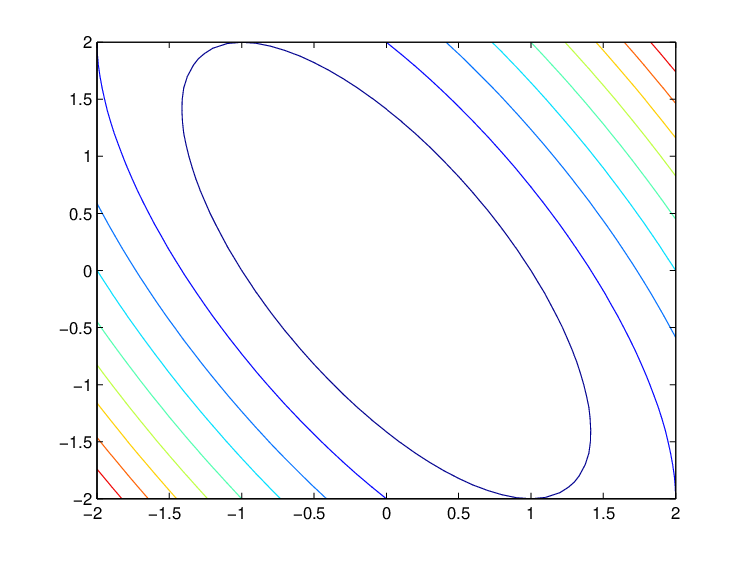
Figure 2. (a) Left: Drift characteristics and flow vector field for the 2D FPE (2.1) with 𝐃=diag⁡(1, 0){\mathbf{D}}=\diag(1,\;0), 𝐂=[1  0; 1  1]\mathbf{C}=[1\;\,0\;;\;1\;\,1]. (b) Right: Level curves of the quadratic potential appearing in the steady state, i.e. A⁡(x)=−ln⁡f∞​(x)A(x)=-\ln f_{\infty}(x).

One easily verifies that the steady state is given by the non-isotropic Gaussian

f∞​(x)=c​e−(x12+2​x1​x2+2​x22),f_{\infty}(x)=c\,\mathrm{e}^{-(x_{1}^{2}+2x_{1}x_{2}+2x_{2}^{2})}\,,

with a normalization constant cc. The contour lines of the steady state potential are graphed in Figure 2b. Here, the “sharp” decay rate is given by 1−ε1-\varepsilon (where min⁡{Re⁡(λ)|λ∈σ⁡(𝐂)}=1\min\{\operatorname{Re}(\lambda)\,|\,\lambda\in\sigma(\mathbf{C})\}=1). □\square

2.3. Steady states and normalized Fokker-Planck equations

In the above examples we saw that, to enable convergence to an equilibrium, the drift matrix 𝐂\mathbf{C} has to mix the diffusive and non-diffusive directions of the linear FPE (2.1) (provided 𝐃{\mathbf{D}} is singular). Now we give conditions on 𝐃{\mathbf{D}} and 𝐂\mathbf{C} such that (2.1) has a unique steady state:

Definition 2.5.

The operator LL from (2.1) is said to fulfill condition (A) if:

  1. (A1)

    No (nontrivial) subspace of ker⁡𝐃\ker{\mathbf{D}} is invariant under 𝐂T\mathbf{C}^{T}.

  2. (A2)

    The matrix 𝐂\mathbf{C} is positively stable (i.e. all eigenvalues have real part greater than zero).

Condition (A1) is equivalent to the hypoellipticity of ∂t−L\partial_{t}-L (cf. §1 of [24]). Moreover, it implies regularization and strict positivity of the solution to (2.1):

Proposition 2.6.

Let condition (A1) from Definition 2.5 hold, and let f0∈L1​(ℝd)f_{0}\in L^{1}(\mathbb{R}^{d}).

  1. a)

    Then the unique solution of (2.1) satisfies f∈C∞​(ℝ+×ℝd)f\in C^{\infty}(\mathbb{R}^{+}\times\mathbb{R}^{d}).

  2. b)

    If f0≥0f_{0}\geq 0, we have f⁡(t,x)>0​∀t>0,x∈ℝdf(t,x)>0\;\;\forall t>0,\,x\in\mathbb{R}^{d}.

Proof.

For part (a) see page 148 of [24]. Part (b) follows from the strict positivity of the Green’s function pertaining to (2.1) (see Lemma 2.5 and Theorem 2.7 in [5]). ∎

Condition (A2) means that there is a confinement potential that prevents the solution to run off to ∞\infty. Without it, there would be no steady state. Indeed, Theorems 2.8 and 2.16 will show that condition (A) is both sufficient and necessary for the existence of a unique normalized steady state and exponential convergence of solutions towards the steady state. So, for equations of type (2.1), hypoellipticity and confinement are equivalent to hypocoercivity.

In the following lemma we give three equivalent characterizations of the hypoellipticity of LL that will be used for the regularization of the propagators eL​t\mathrm{e}^{Lt}, t>0t>0 (see Theorem 2.15 below, and §2 of [31]).

Lemma 2.7.

The following three statements are equivalent, where we use k:=rank⁡𝐃∈{1,…,d}k:=\operatorname{rank}{\mathbf{D}}\in\{1,\dots,d\}:

  • (i)

    No non-trivial subspace of ker⁡𝐃\ker{\mathbf{D}} is invariant under 𝐂T\mathbf{C}^{T}.

  • (ii)

    There exist constants τ∈{0,…,d−k}\tau\in\{0,\dots,d-k\} and κ>0\kappa>0 such that

    (2.28) ∑j=0τ𝐂j​𝐃​(𝐂T)j≥κ​𝐈.\displaystyle\sum\limits_{j=0}^{\tau}\mathbf{C}^{j}{\mathbf{D}}(\mathbf{C}^{T})^{j}\geq\kappa\mathbf{I}\,.
  • (iii)

    There exists a constant τ∈{0,…,d−k}\tau\in\{0,\dots,d-k\} such that

    (2.29) rank⁡[𝐃12,𝐂𝐃12,…,𝐂τ​𝐃12]=d.\displaystyle\operatorname{rank}[{\mathbf{D}}^{\frac{1}{2}},\,\mathbf{C}{\mathbf{D}}^{\frac{1}{2}},...,\,\mathbf{C}^{\tau}{\mathbf{D}}^{\frac{1}{2}}]=d\,.
Proof.

For the equivalence of (i) and (ii) we refer to Lemma 2.3 of [5].
For (iii)⇒\Rightarrow(ii) let

𝐄:=[𝐃12,𝐂𝐃12,…,𝐂τ​𝐃12]∈ℝd×(τ+1)​d.\mathbf{E}:=[{\mathbf{D}}^{\frac{1}{2}},\,\mathbf{C}{\mathbf{D}}^{\frac{1}{2}},...,\,\mathbf{C}^{\tau}{\mathbf{D}}^{\frac{1}{2}}]\in\mathbb{R}^{d\times(\tau+1)d}\,.

Then,

ℝd×d∋𝐄​𝐄T=∑j=0τ𝐂j​𝐃​(𝐂T)j≥𝟎\mathbb{R}^{d\times d}\ni\mathbf{E}\ \mathbf{E}^{T}=\sum\limits_{j=0}^{\tau}\mathbf{C}^{j}{\mathbf{D}}(\mathbf{C}^{T})^{j}\geq\mathbf{0}

has rank dd and (2.28) follows.
For (ii)⇒\Rightarrow(iii) assume we had rank⁡𝐄T<d\operatorname{rank}\mathbf{E}^{T}<d. Then, ∃ 0≠v∈ℝd\exists\,0\neq v\in\mathbb{R}^{d} with 𝐄T​v=0\mathbf{E}^{T}v=0. Hence, 𝐄​𝐄T​v=0\mathbf{E}\ \mathbf{E}^{T}v=0 would contradict (2.28). ∎

If τ\tau is the minimal constant for which (2.28) (or, equivalently, (2.29)) holds, then LL fulfills Hörmander’s finite rank bracket condition of order τ\tau (see [24], Theorem 1.1). For the explicit decomposition of the generator from (2.1) in the Hörmander form −L=A∗​A+B-L=A^{*}A+B we refer to Proposition 5 in [41].

As an illustration we consider the following two hypocoercive examples of (2.1), where d=4,k=2d=4,\,k=2:

Example 2.4.

Let

𝐃1:=(1000010000000000);\displaystyle{\mathbf{D}}_{1}:=\left(\begin{array}[]{cccc}1&0&0&0\\ 0&1&0&0\\ 0&0&0&0\\ 0&0&0&0\end{array}\right); 𝐂1:=(10100101−10000−100).\displaystyle\quad\mathbf{C}_{1}:=\left(\begin{array}[]{cccc}1&0&1&0\\ 0&1&0&1\\ -1&0&0&0\\ 0&-1&0&0\end{array}\right)\,.

Here, rank⁡[𝐃112,𝐂1​𝐃112]=4\operatorname{rank}[{\mathbf{D}}_{1}^{\frac{1}{2}},\,\mathbf{C}_{1}{\mathbf{D}}_{1}^{\frac{1}{2}}]=4 and hence τ=1\tau=1. □\square

Example 2.5.

Let

𝐃2:=(1000010000000000);\displaystyle{\mathbf{D}}_{2}:=\left(\begin{array}[]{cccc}1&0&0&0\\ 0&1&0&0\\ 0&0&0&0\\ 0&0&0&0\end{array}\right); 𝐂2:=(100001100−10100−10).\displaystyle\quad\mathbf{C}_{2}:=\left(\begin{array}[]{cccc}1&0&0&0\\ 0&1&1&0\\ 0&-1&0&1\\ 0&0&-1&0\end{array}\right)\,.

Here, rank⁡[𝐃212,𝐂2​𝐃212]=3\operatorname{rank}[{\mathbf{D}}_{2}^{\frac{1}{2}},\,\mathbf{C}_{2}{\mathbf{D}}_{2}^{\frac{1}{2}}]=3, but rank⁡[𝐃212,𝐂2​𝐃212,𝐂22​𝐃212]=4\operatorname{rank}[{\mathbf{D}}_{2}^{\frac{1}{2}},\,\mathbf{C}_{2}{\mathbf{D}}_{2}^{\frac{1}{2}},\,\mathbf{C}_{2}^{2}{\mathbf{D}}_{2}^{\frac{1}{2}}]=4. Hence τ=2\tau=2. □\square

In many works on hypocoercive equations [17, 12], a more restrictive assumption (than condition (A)) is made, namely: “No subspace of ker⁡𝐃\ker{\mathbf{D}} should be mapped into ker⁡𝐃\ker{\mathbf{D}} by 𝐂T\mathbf{C}^{T}”, which corresponds to the requirement τ=1\tau=1. Let as reconsider the two previous examples under this aspect. In Example 2.4, 𝐂1T\mathbf{C}^{T}_{1} maps the non-diffusive directions from ker⁡𝐃1\ker{\mathbf{D}}_{1} into the diffusive directions from (ker⁡𝐃1)⟂(\ker{\mathbf{D}}_{1})^{\perp}. But in Example 2.5, 𝐂2T\mathbf{C}^{T}_{2} maps the non-diffusive direction (0, 0, 0, 1)T∈ker⁡𝐃2(0,\,0,\,0,\,1)^{T}\in\ker{\mathbf{D}}_{2} still onto the non-diffusive direction (0, 0, 1, 0)T∈ker⁡𝐃2(0,\,0,\,1,\,0)^{T}\in\ker{\mathbf{D}}_{2}. But in a second step, we have 𝐂2T​(0, 0, 1, 0)T=(0, 1, 0,−1)T\mathbf{C}^{T}_{2}(0,\,0,\,1,\,0)^{T}=(0,\,1,\,0,\,-1)^{T}, which has a nontrivial component in the diffusive subspace (ker⁡𝐃2)⟂(\ker{\mathbf{D}}_{2})^{\perp}.

Next we discuss the existence of a steady state to (2.1) (for the proof cf. §1 of [31] or Th. 3.1 in [5]):

Theorem 2.8.

There exists a unique steady state f∞∈L1​(ℝd)f_{\infty}\in L^{1}(\mathbb{R}^{d}) of (2.1) fulfilling ∫ℝdf∞​d⁡x=1\int_{\mathbb{R}^{d}}f_{\infty}\,\operatorname{d}\!x=1 iff condition (A) holds.
Moreover, this steady state is of the (non-isotropic) Gaussian form

(2.30) f∞​(x)\displaystyle f_{\infty}(x) =cK​exp⁡(−xT​𝐊−1​x2),\displaystyle=c_{K}\exp\Big(-\frac{x^{T}\mathbf{K}^{-1}x}{2}\Big),

where 𝐊\mathbf{K} is the unique, symmetric, and positive definite solution to the continuous Lyapunov equation (cf. [25])

(2.31) 2​𝐃=𝐂𝐊+𝐊𝐂T,\displaystyle 2{\mathbf{D}}=\mathbf{C}\mathbf{K}+\mathbf{K}\mathbf{C}^{T},

and cK=(2​π)−d2​(det𝐊)−12c_{K}=(2\pi)^{-\frac{d}{2}}(\det\mathbf{K})^{-\frac{1}{2}} is the normalization constant.

With the steady state at hand, we now give the decomposition of the operator LL from (2.1):

Lemma 2.9.

Let LL satisfy condition (A). Then, its symmetric/anti-symmetric decomposition satisfies:

(2.32) Ls​f\displaystyle L_{s}f =div(f∞𝐃∇ff∞),\displaystyle=\operatorname{div}\Big(f_{\infty}{\mathbf{D}}\nabla\frac{f}{f_{\infty}}\Big)\,,
(2.33) La​s​f\displaystyle L_{as}f =div(f∞𝐑∇ff∞),\displaystyle=\operatorname{div}\Big(f_{\infty}\mathbf{R}\nabla\frac{f}{f_{\infty}}\Big)\,,

with 𝐑:=12​(𝐂𝐊−𝐊𝐂T)≠𝟎\mathbf{R}:=\frac{1}{2}(\mathbf{C}\mathbf{K}-\mathbf{K}\mathbf{C}^{T})\neq\mathbf{0}.

Proof.

To reduce this result to Lemma 2.1, we first compare (2.1) to (2.10): The drift vector field 𝐂​x\mathbf{C}x of (2.1) corresponds to 𝐃​{∇A+F}{\mathbf{D}}\{\nabla A+F\}. Hence, we have with (2.31) and ∇A=𝐊−1​x\nabla A=\mathbf{K}^{-1}x:

𝐃​F​(x)\displaystyle{\mathbf{D}}F(x) =𝐂x−𝐃∇A(x)=[𝐂−12(𝐂𝐊+𝐊𝐂T)𝐊−1]x\displaystyle=\mathbf{C}x-{\mathbf{D}}\nabla A(x)=\big[\mathbf{C}-\frac{1}{2}(\mathbf{C}\mathbf{K}+\mathbf{K}\mathbf{C}^{T})\mathbf{K}^{-1}\big]x
(2.34) =12​(𝐂𝐊−𝐊𝐂T)​𝐊−1​x.\displaystyle=\frac{1}{2}(\mathbf{C}\mathbf{K}-\mathbf{K}\mathbf{C}^{T})\mathbf{K}^{-1}x\,.

To verify the divergence-free-condition (2.11) we compute

div⁡(𝐃​F​(x)​f∞​(x))\displaystyle\!\!\!\!\operatorname{div}({\mathbf{D}}F(x)\ f_{\infty}(x))
=12​Tr⁡([𝐂𝐊−𝐊𝐂T]​𝐊−1)​f∞−12​(𝐊−1​x)T​[𝐂𝐊−𝐊𝐂T]​𝐊−1​x​f∞=0,\displaystyle=\frac{1}{2}\tr([\mathbf{C}\mathbf{K}-\mathbf{K}\mathbf{C}^{T}]\mathbf{K}^{-1})\,f_{\infty}-\frac{1}{2}(\mathbf{K}^{-1}x)^{T}\,[\mathbf{C}\mathbf{K}-\mathbf{K}\mathbf{C}^{T}]\,\mathbf{K}^{-1}x\,f_{\infty}=0\,,

due to the skew-symmetry of 𝐂𝐊−𝐊𝐂T\mathbf{C}\mathbf{K}-\mathbf{K}\mathbf{C}^{T}.

Next we verify the condition (2.14):

(∇T(𝐑f∞))T=−𝐑∇f∞=12(𝐂𝐊−𝐊𝐂T)𝐊−1xf∞=𝐃F(x)f∞(x),(\nabla^{T}(\mathbf{R}f_{\infty}))^{T}=-\mathbf{R}\nabla f_{\infty}=\frac{1}{2}(\mathbf{C}\mathbf{K}-\mathbf{K}\mathbf{C}^{T})\mathbf{K}^{-1}x\,f_{\infty}={\mathbf{D}}F(x)f_{\infty}(x)\,,

where we used (2.34) in the last step. The claims (2.32), (2.33) then follow from Lemma 2.1.

Finally we prove that 𝐑≠𝟎\mathbf{R}\neq\mathbf{0}. Otherwise (2.31) would imply 𝐃=𝐊𝐂T{\mathbf{D}}=\mathbf{K}\mathbf{C}^{T}, and hence ker⁡𝐃=ker⁡𝐂T\ker{\mathbf{D}}=\ker\mathbf{C}^{T}, which would contradict condition (A). ∎

The result 𝐑≠𝟎\mathbf{R}\neq\mathbf{0} shows that hypocoercive FPEs of form (2.1) are always non-symmetric.

Next we shall bring the hypocoercive FPEs (2.1) to a normalized form, which will simplify our computations below. With its steady state given in (2.30) we introduce, as a first step, the coordinate transformation y:=𝐊−1​x∈ℝdy:=\sqrt{\mathbf{K}}^{\,-1}x\in\mathbb{R}^{d}. With g⁡(y):=f⁡(𝐊​y)g(y):=f(\sqrt{\mathbf{K}}y), this transforms (2.1) to

∂tg=divy⁡(𝐃~​∇yg+𝐂~​y​g),\partial_{t}g=\operatorname{div}_{y}(\widetilde{\mathbf{D}}\nabla_{y}g+\widetilde{\mathbf{C}}y\,g)\,,

with 𝐃~=𝐊−1​𝐃​𝐊−1\widetilde{\mathbf{D}}=\sqrt{\mathbf{K}}^{\,-1}{\mathbf{D}}\sqrt{\mathbf{K}}^{\,-1} and 𝐂~=𝐊−1​𝐂​𝐊\widetilde{\mathbf{C}}=\sqrt{\mathbf{K}}^{\,-1}\mathbf{C}\sqrt{\mathbf{K}}. A simple computation, using (2.31) shows that

𝐃~=𝐂~s,\widetilde{\mathbf{D}}=\widetilde{\mathbf{C}}_{s}\,,

where 𝐂~s:=12​(𝐂~+𝐂~T)\widetilde{\mathbf{C}}_{s}:=\frac{1}{2}(\widetilde{\mathbf{C}}+\widetilde{\mathbf{C}}^{T}) denotes the symmetric part of 𝐂~\widetilde{\mathbf{C}}. Clearly, the transformed steady state reads g∞(y)=ce−|y|2/2g_{\infty}(y)=c\,\mathrm{e}^{-|y|^{2}/2}, with some normalization constant c>0c>0. As a second step we rotate the coordinate system to diagonalize the diffusion matrix: For an orthogonal matrix 𝐔∈ℝd×d\mathbf{U}\in\mathbb{R}^{d\times d}, let 𝐃^:=𝐔T​𝐃~​𝐔=diag​(d1,…,dk, 0,…, 0)\widehat{\mathbf{D}}:=\mathbf{U}^{T}\widetilde{\mathbf{D}}\mathbf{U}=\mbox{diag}(d_{1},\,...,\,d_{k},\,0\,,...,\,0), where k=rank⁡𝐃k=\operatorname{rank}{\mathbf{D}}. We set z:=𝐔T​yz:=\mathbf{U}^{T}y and h⁡(z):=g⁡(𝐔​z)h(z):=g(\mathbf{U}z), which satisfies

(2.35) ∂th=divz⁡(𝐃^​∇zh+𝐂^​z​h).\partial_{t}h=\operatorname{div}_{z}(\widehat{{\mathbf{D}}}\nabla_{z}h+\widehat{\mathbf{C}}z\,h)\,.

The symmetric part of the new drift matrix, 𝐂^=𝐔T​𝐂~​𝐔\widehat{\mathbf{C}}=\mathbf{U}^{T}\widetilde{\mathbf{C}}\mathbf{U}, again satisfies 𝐃^=𝐂^s\widehat{{\mathbf{D}}}=\widehat{\mathbf{C}}_{s}. Since the matrices 𝐂\mathbf{C} and 𝐂^\widehat{\mathbf{C}} are similar, we have σ⁡(𝐂)=σ⁡(𝐂^)\sigma(\mathbf{C})=\sigma(\widehat{\mathbf{C}}), which will be the quantity that determines the decay rate of a hypocoercive FPE. We also note that h∞(z)=ce−|z|2/2h_{\infty}(z)=c\,\mathrm{e}^{-|z|^{2}/2} with some normalization constant cc.

We remark that the above Examples 2.2, 2.4, and 2.5 are already of this normalized form, but Example 2.3 is not. The above normalization brings Example 2.3 to the form

∂th=divz⁡[(2000)​∇zh+(21−10)​z​h].\partial_{t}h=\operatorname{div}_{z}\Big[\left(\begin{array}[]{cc}2&0\\ 0&0\end{array}\right)\nabla_{z}h+\left(\begin{array}[]{cc}2&1\\ -1&0\end{array}\right)z\,h\Big]\,.

Scaling time by a factor 12\frac{1}{2} shows that this equals the FPE in Example 2.2 with the rotation parameter ω=−12\omega=-\frac{1}{2}, which is a limiting case in (2.27).

For the rest of this chapter we shall always assume that the FPEs are normalized as in (2.35). So, the matrices in (2.1) will satisfy 𝐃=𝐂s{\mathbf{D}}=\mathbf{C}_{s} with 𝐃{\mathbf{D}} being diagonal, which implies 𝐊=𝐈\mathbf{K}=\mathbf{I}.

2.4. Modified entropy method

To start with, let us very briefly review the standard entropy method for FPEs (cf. [10, 7] for symmetric FPEs and [2, 13] for non-symmetric FPEs): In a first step one establishes a differential inequality between the Fisher information (2.18) of a solution f⁡(t)f(t) and its time derivative, which yields exponential decay of the Fisher information. We give the result for symmetric FPEs:

Lemma 2.10.

Let f⁡(t)f(t) be the solution to (2.8) with a constant diffusion matrix 𝐃{\mathbf{D}}. Let the coefficients of this FPE satisfy the following Bakry-Émery condition for some λ1>0\lambda_{1}>0:

(2.36) ∂2A∂x2​(x)≥λ1​𝐃−1,∀x∈ℝd.\frac{\partial^{2}A}{\partial x^{2}}(x)\geq\lambda_{1}{\mathbf{D}}^{-1}\,,\quad\forall\,x\in\mathbb{R}^{d}\,.

Also, let the initial condition satisfy Iψ​(f0|f∞)<∞I_{\psi}(f_{0}|f_{\infty})<\infty. Then, the Fisher information decays exponentially:

(2.37) Iψ​(f⁡(t)|f∞)≤e−2​λ1​t​Iψ​(f0|f∞),t≥0.I_{\psi}(f(t)|f_{\infty})\leq\mathrm{e}^{-2\lambda_{1}t}I_{\psi}(f_{0}|f_{\infty})\,,\quad t\geq 0\,.
Proof.

After a lengthy computation the time derivative of the Fisher information can be written as follows (for scalar diffusions D⁡(x)D(x) cf. Lemma 2.13 in [7], and for the generalization to non-symmetric FPEs (2.10) cf. Lemma 2.3 in [2]). Using the notation u:=∇ff∞u:=\nabla\frac{f}{f_{\infty}} we have:

dd⁡t​Iψ​(f⁡(t))\displaystyle\frac{\,\operatorname{d}\!}{\,\operatorname{d}\!t}I_{\psi}(f(t)) =−2∫ℝdψ′′(ff∞)uT𝐃∂2A∂x2𝐃uf∞dx−2∫ℝdTr(𝐗𝐘)f∞dx\displaystyle=-2\int_{\mathbb{R}^{d}}{\psi^{\prime\prime}\Big(\frac{f}{f_{\infty}}\Big)\ u^{T}{\mathbf{D}}\frac{\partial^{2}A}{\partial x^{2}}{\mathbf{D}}u\,f_{\infty}\,\operatorname{d}\!x}-2\int_{\mathbb{R}^{d}}\tr{(\mathbf{X}\mathbf{Y})}\,f_{\infty}\,\operatorname{d}\!x
(2.38) ≤−2λ1∫ℝdψ′′(ff∞)uT𝐃uf∞dx=−2λ1Iψ(f(t)).\displaystyle\leq-2\lambda_{1}\int_{\mathbb{R}^{d}}{\psi^{\prime\prime}\Big(\frac{f}{f_{\infty}}\Big)\ u^{T}{\mathbf{D}}u\,f_{\infty}\,\operatorname{d}\!x}=-2\lambda_{1}\,I_{\psi}(f(t))\,.

In the last estimate we used the Bakry-Émery condition (2.36) and Tr⁡(𝐗𝐘)≥0\tr{(\mathbf{X}\mathbf{Y})}\geq 0. Here, the two matrices 𝐗,𝐘∈ℝ2×2\mathbf{X},\,\mathbf{Y}\in\mathbb{R}^{2\times 2} are defined as follows:

𝐗⁡(x)\displaystyle\mathbf{X}(x) :=(ψ′′ψ′′′ψ′′′12​ψI​V)​(f⁡(x)f∞​(x))≥𝟎,∀x∈ℝd,\displaystyle:=\left(\begin{array}[]{cc}\psi^{\prime\prime}&\psi^{\prime\prime\prime}\\ \psi^{\prime\prime\prime}&\frac{1}{2}\psi^{IV}\end{array}\right)\Big(\frac{f(x)}{f_{\infty}(x)}\Big)\geq\mathbf{0}\,,\quad\forall\,x\in\mathbb{R}^{d}\,,

since det𝐗=12​ψ′′​ψI​V−(ψ′′)2≥0\det\,\mathbf{X}=\frac{1}{2}\psi^{\prime\prime}\psi^{IV}-(\psi^{\prime\prime})^{2}\geq 0 for admissible relative entropies (cf. (2.16)).

𝐘⁡(x)\displaystyle\mathbf{Y}(x) :=(Tr⁡[(𝐃​∂u∂x)2]uT​𝐃​∂u∂x​𝐃​uuT​𝐃​∂u∂x​𝐃​u(uT​𝐃​u)2)≥𝟎,∀x∈ℝd,\displaystyle:=\left(\begin{array}[]{cc}\tr\big[\big({\mathbf{D}}\frac{\partial u}{\partial x}\big)^{2}\big]&u^{T}{\mathbf{D}}\frac{\partial u}{\partial x}{\mathbf{D}}u\\[5.69054pt] u^{T}{\mathbf{D}}\frac{\partial u}{\partial x}{\mathbf{D}}u&(u^{T}{\mathbf{D}}u)^{2}\end{array}\right)\geq\mathbf{0}\,,\quad\forall\,x\in\mathbb{R}^{d}\,,

due to the Cauchy-Schwarz inequality. The differential inequality (2.38) for Iψ​(f​(t))I_{\psi}(f(t)) implies (2.37), and it can be written equivalently as e′′​(t)≥−2​λ1​e′​(t)e^{\prime\prime}(t)\geq-2\lambda_{1}e^{\prime}(t) (with e⁡(t):=eψ​(f⁡(t)|f∞)e(t):=e_{\psi}(f(t)|f_{\infty})). ∎

In the second step of the entropy method one proves the exponential decay of the relative entropy (2.17) of f⁡(t)f(t) w.r.t. f∞f_{\infty}. To this end one integrates (2.38) from tt to ∞\infty, which yields the entropy inequality

(2.43) dd⁡t​eψ​(f⁡(t)|f∞)≤−2​λ1​eψ​(f⁡(t)|f∞),∀t≥0.\frac{\,\operatorname{d}\!}{\,\operatorname{d}\!t}e_{\psi}(f(t)|f_{\infty})\leq-2\lambda_{1}\,e_{\psi}(f(t)|f_{\infty})\,,\quad\forall\,t\geq 0\,.

Hence, the relative entropy decays exponentially:

(2.44) eψ​(f⁡(t)|f∞)≤e−2​λ1​t​eψ​(f0|f∞),∀t≥0.e_{\psi}(f(t)|f_{\infty})\leq\mathrm{e}^{-2\lambda_{1}t}e_{\psi}(f_{0}|f_{\infty})\,,\quad\forall\,t\geq 0\,.
Refer to caption
Figure 3. Prototypical behavior of the logarithmic relative entropy e1​(f⁡(t)|f∞)e_{1}(f(t)|f_{\infty}) (solid red curve), its first (dotted black), and second time derivative (dashed blue) for a non-degenerate, symmetric FPE: The inequalities e′≤−2​λ​ee^{\prime}\leq-2\lambda e, e′′≥−2​λ​e′e^{\prime\prime}\geq-2\lambda e^{\prime} can be obtained. (colors only online)
Refer to caption
Figure 4. Prototypical behavior of the logarithmic relative entropy e1​(f⁡(t)|f∞)e_{1}(f(t)|f_{\infty}) (solid red curve), its first (dotted black), and second time derivative (dashed blue) for the degenerate, hypocoercive FPE from Example 2.2 with 𝐃=diag⁡(1, 0){\mathbf{D}}=\diag(1,\,0), 𝐂=[1−1; 1 0]\mathbf{C}=[1\;-1\,;\,1\;0] : The inequalities e′≤−2​λ​ee^{\prime}\leq-2\lambda e, e′′≥−2​λ​e′e^{\prime\prime}\geq-2\lambda e^{\prime} are wrong, in general. (colors only online)

Next we illustrate how the situation changes from a symmetric FPE to a non-symmetric or even hypocoercive FPE. In a symmetric FPE with 𝐃>0{\mathbf{D}}>0, the relative entropy is a convex function of time, and the entropy dissipation satisfies eψ′​(f|f∞)<0e^{\prime}_{\psi}(f|f_{\infty})<0 for all probability densities f≠f∞f\neq f_{\infty} (cf. Figure 3). For a hypocoercive FPE with a singular diffusion matrix 𝐃{\mathbf{D}}, however, e⁡(t)e(t) is not convex. In fact, it decays in a “wavy” fashion, and it may have horizontal tangents at equally spaced points in time (cf. Figure 4). This oscillatory behavior is also known from space-inhomogeneous kinetic equations (cf. §3.7 of [40]; and [19] for a numerical study on the Boltzmann equation).

So we observe that the entropy dissipation eψ′​(f|f∞)e^{\prime}_{\psi}(f|f_{\infty}) may vanish for certain probability densities f≠f∞f\neq f_{\infty}. This can also be seen from the form of the Fisher information in (2.18): choose f⁡(x)=(1+c⋅x)​f∞​(x)f(x)=(1+c\cdot x)f_{\infty}(x) with a vector c∈ker⁡𝐃c\in\ker{\mathbf{D}}. Hence, an entropy inequality of the form (2.43) cannot hold for degenerate, hypocoercive FPEs! We also see: While the Fisher information Iψ​(f⁡(t)|f∞)I_{\psi}(f(t)|f_{\infty}) is a Lyapunov functional for symmetric FPEs, its non-monotonicity in the hypocoercive case makes it “useless” there. As a remedy, we present now a modified entropy method for FPEs of the form (2.1), normalized as introduced in §2.3.

Since the above problems stem from the singularity of 𝐃{\mathbf{D}}, we now define a modified entropy dissipation functional:

(2.45) Sψ​(f):=∫ℝdψ′′​(ff∞)​(∇ff∞)T​𝐏​(∇ff∞)​f∞​d⁡x≥0,S_{\psi}(f):=\int_{\mathbb{R}^{d}}\psi^{\prime\prime}\Big(\frac{f}{f_{\infty}}\Big)\ \Big(\nabla\frac{f}{f_{\infty}}\Big)^{T}\mathbf{P}\Big(\nabla\frac{f}{f_{\infty}}\Big)\,f_{\infty}\,\,\operatorname{d}\!x\geq 0\,,

where the positive definite matrix 𝐏∈ℝd×d\mathbf{P}\in\mathbb{R}^{d\times d} still has to be determined. Note that the only difference to the Fisher information is the replacement of the matrix 𝐃{\mathbf{D}} there by 𝐏\mathbf{P} here. This auxiliary functional will take over the role of IψI_{\psi} in the first step of the entropy method. So, our goal is to derive a differential inequality between Sψ​(f​(t))S_{\psi}(f(t)) and dd⁡t​Sψ​(f⁡(t))\frac{\,\operatorname{d}\!}{\,\operatorname{d}\!t}S_{\psi}(f(t)) for a “good” choice of 𝐏>0\mathbf{P}>0. Then, once exponential decay of Sψ​(f​(t))S_{\psi}(f(t)) is obtained, the trivial estimate 𝐏≥cP​𝐃\mathbf{P}\geq c_{P}{\mathbf{D}} (with some cP>0c_{P}>0) implies

Sψ​(f⁡(t))≥cP​Iψ​(f⁡(t)|f∞),S_{\psi}(f(t))\geq c_{P}I_{\psi}(f(t)|f_{\infty})\,,

and also exponential decay of Iψ​(f​(t))I_{\psi}(f(t)) follows.

The key question for using the modified entropy dissipation functional Sψ​(f)S_{\psi}(f) is how to choose the matrix 𝐏\mathbf{P} for a given, normalized FPE. To determine 𝐏\mathbf{P} we shall need the following algebraic result:

Lemma 2.11.

For any fixed matrix 𝐐∈ℝd×d\mathbf{Q}\in\mathbb{R}^{d\times d}, let μ:=min{Re{λ}|λ\mu:=\min\{\operatorname{Re}\{\lambda\}|\lambda is an eigenvalue of 𝐐}\mathbf{Q}\}. Let {λm|1≤m≤m0}\{\lambda_{m}|1\leq m\leq m_{0}\} be all the eigenvalues of 𝐐\mathbf{Q} with Re⁡{λm}=μ\operatorname{Re}\{\lambda_{m}\}=\mu, only counting their geometric multiplicity.

  • (i)

    If all λm\lambda_{m}, m∈{1,…,m0}m\in\{1,\dots,m_{0}\}, are non-defective11 1 An eigenvalue is defective if its geometric multiplicity is strictly less than its algebraic multiplicity., then there exists a symmetric, positive definite matrix 𝐏∈ℝd×d\mathbf{P}\in\mathbb{R}^{d\times d} with

    (2.46) 𝐏𝐐+𝐐T​𝐏\displaystyle\mathbf{P}\mathbf{Q}+\mathbf{Q}^{T}\mathbf{P} ≥2​μ​𝐏.\displaystyle\geq 2\mu\mathbf{P}\,.
  • (ii)

    If λm\lambda_{m} is defective for at least one m∈{1,…,m0}m\in\{1,\dots,m_{0}\}, then for any ε>0\varepsilon>0 there exists a symmetric, positive definite matrix 𝐏=𝐏⁡(ε)∈ℝd×d\mathbf{P}=\mathbf{P}(\varepsilon)\in\mathbb{R}^{d\times d} with

    (2.47) 𝐏𝐐+𝐐T​𝐏\displaystyle\mathbf{P}\mathbf{Q}+\mathbf{Q}^{T}\mathbf{P} ≥2​(μ−ε)​𝐏.\displaystyle\geq 2(\mu-\varepsilon)\mathbf{P}\,.
Proof.

Here we only give the proof for the case that 𝐐\mathbf{Q} is not defective (and hence diagonalizable) and refer to Lemma 4.3 in [5] for the general case. Let w1,…,wdw_{1},\dots,w_{d} denote the eigenvectors of 𝐐T\mathbf{Q}^{T}. Then one can choose 𝐏\mathbf{P} as a weighted sum of the following rank 1 matrices:

(2.48) 𝐏:=∑j=1dbj​wj⊗wj¯T,\displaystyle\mathbf{P}:=\sum\limits_{j=1}^{d}b_{j}\,w_{j}\otimes\overline{w_{j}}^{T}\,,

with bj∈ℝ+b_{j}\in\mathbb{R}^{+}; j=1,…,dj=1,\dots,d. As {wj}j=1,…,d\{w_{j}\}_{j=1,\dots,d} is a basis of ℂd\mathbb{C}^{d}, 𝐏\mathbf{P} is positive definite. If any wjw_{j} is complex, its complex conjugate wj¯\overline{w_{j}} is also an eigenvector of 𝐐T\mathbf{Q}^{T}, since 𝐐\mathbf{Q} is real. By taking the same coefficient bjb_{j} for both, we obtain a real matrix 𝐏\mathbf{P}. Apart from this restriction, the choice of bj>0b_{j}>0 is arbitrary. For 𝐏\mathbf{P} from (2.48), we have

𝐏𝐐+𝐐T​𝐏\displaystyle\mathbf{P}\mathbf{Q}+\mathbf{Q}^{T}\mathbf{P} =∑j=1dbj​(λj¯+λj)​wj⊗wj¯T≥2​μ​∑j=1dbj​wj⊗wj¯T=2​μ​𝐏.\displaystyle=\sum\limits_{j=1}^{d}b_{j}(\overline{\lambda_{j}}+\lambda_{j})w_{j}\otimes\overline{w_{j}}^{T}\geq 2\mu\sum\limits_{j=1}^{d}b_{j}\,w_{j}\otimes\overline{w_{j}}^{T}=2\mu\mathbf{P}\,.

∎

We remark that 𝐏\mathbf{P} is, in general, not unique, not even up to a multiplicative constant. But this will be irrelevant for the decay rate of FPEs.

Applying this lemma to 𝐐:=𝐂\mathbf{Q}:=\mathbf{C} now yields exponential decay of the functional Sψ​(f​(t))S_{\psi}(f(t)), defined with the matrix 𝐏\mathbf{P} from the above lemma:

Proposition 2.12.

Assume condition (A). Let ψ\psi generate an admissible entropy, let ff be the solution to (2.1) with an initial state satisfying Sψ​(f0)<∞S_{\psi}(f_{0})<\infty, and let μ:=min⁡{Re⁡{λ}|λ​ is an eigenvalue of ​𝐂}\mu:=\min\left\{\operatorname{Re}\{\lambda\}|\lambda\text{ is an eigenvalue of }\mathbf{C}\right\} (which is positive by condition (A)). Let {λm|1≤m≤m0}\{\lambda_{m}|1\leq m\leq m_{0}\} be the eigenvalues of 𝐂\mathbf{C} with Re⁡{λm}=μ\operatorname{Re}\{\lambda_{m}\}=\mu, and let 𝐏\mathbf{P} be defined as in Lemma 2.11.

  • (i)

    If all λm\lambda_{m}, 1≤m≤m01\leq m\leq m_{0}, are non-defective, then

    Sψ​(f​(t))\displaystyle S_{\psi}(f(t)) ≤Sψ​(f0)​e−2​μ​t,t≥0.\displaystyle\leq S_{\psi}(f_{0})\mathrm{e}^{-2\mu t},\quad t\geq 0.
  • (ii)

    If λm\lambda_{m} is defective for at least one m∈{1,…,m0}m\in\{1,\dots,m_{0}\}, then

    Sψ​(f​(t),ε)\displaystyle S_{\psi}(f(t),\varepsilon) ≤Sψ​(f0,ε)​e−2​(μ−ε)​t,t≥0,\displaystyle\leq S_{\psi}(f_{0},\varepsilon)\mathrm{e}^{-2(\mu-\varepsilon)t},\quad t\geq 0,

    for any ε∈(0,μ)\varepsilon\in(0,\mu). Here, Sψ​(f,ε)S_{\psi}(f,\varepsilon) denotes the modified entropy dissipation functional (2.45) with the matrix 𝐏=𝐏⁡(ε)\mathbf{P}=\mathbf{P}(\varepsilon).

Proof.

In a tedious computation the time derivative of the functional S⁡(ψ⁡(f⁡(t))CLOSES(\psi(f(t)) can be written as follows (cf. Proposition 4.5 in [5]). Using the notation u:=∇ff∞u:=\nabla\frac{f}{f_{\infty}} we have:

dd⁡t​Sψ​(f⁡(t))=\displaystyle\frac{\,\operatorname{d}\!}{\,\operatorname{d}\!t}S_{\psi}(f(t))= −2∫ℝdψ′′(ff∞)uT[𝐏𝐂+𝐂T𝐏]uf∞dx\displaystyle-2\int_{\mathbb{R}^{d}}{\psi^{\prime\prime}\Big(\frac{f}{f_{\infty}}\Big)\ u^{T}\big[\mathbf{P}\mathbf{C}+\mathbf{C}^{T}\mathbf{P}\big]u\,f_{\infty}\,\operatorname{d}\!x}
(2.49) −2∫ℝdTr(𝐗𝐘P)f∞dx\displaystyle-2\int_{\mathbb{R}^{d}}\tr{(\mathbf{X}\mathbf{Y}_{P})}\,f_{\infty}\,\operatorname{d}\!x
≤\displaystyle\leq −2κ∫ℝdψ′′(ff∞)uT𝐏uf∞dx=−2κSψ(f(t)),\displaystyle-2\kappa\int_{\mathbb{R}^{d}}{\psi^{\prime\prime}\Big(\frac{f}{f_{\infty}}\Big)\ u^{T}\mathbf{P}u\,f_{\infty}\,\operatorname{d}\!x}=-2\kappa\,S_{\psi}(f(t))\,,

where κ:=μ\kappa:=\mu for case (i), and κ:=μ−ε\kappa:=\mu-\varepsilon for the defective case (ii). In the last estimate we used the matrix inequality (2.46) in case (i) and (2.47) for case (ii). This inequality replaces the Bakry-Émery condition (2.36) used in the standard entropy method (compare to the estimate (2.38)). In (2.49) we also used Tr⁡(𝐗𝐘P)≥0\tr{(\mathbf{X}\mathbf{Y}_{P})}\geq 0, where the matrix 𝐗\mathbf{X} is defined in (2.4), and the matrix 𝐘P∈ℝ2×2\mathbf{Y}_{P}\in\mathbb{R}^{2\times 2} is now defined as follows:

𝐘P​(x)\displaystyle\mathbf{Y}_{P}(x) :=(Tr⁡(𝐃​∂u∂x​𝐏​∂u∂x)uT​𝐃​∂u∂x​𝐏​uuT​𝐃​∂u∂x​𝐏​u(uT​𝐏​u)​(uT​𝐃​u))≥𝟎,∀x∈ℝd.\displaystyle:=\left(\begin{array}[]{cc}\tr{\big({\mathbf{D}}\frac{\partial u}{\partial x}\mathbf{P}\frac{\partial u}{\partial x}\big)}&u^{T}{\mathbf{D}}\frac{\partial u}{\partial x}\mathbf{P}u\\[5.69054pt] u^{T}{\mathbf{D}}\frac{\partial u}{\partial x}\mathbf{P}u&(u^{T}\mathbf{P}u)(u^{T}{\mathbf{D}}u)\end{array}\right)\geq\mathbf{0}\,,\quad\forall\,x\in\mathbb{R}^{d}\,.

The positivity of 𝐘P\mathbf{Y}_{P} follows from the Cauchy-Schwarz inequality using (uT​𝐃​∂u∂x​𝐏​u)2=Tr⁡(𝐏​(u⊗uT)​𝐃​𝐃​∂u∂x​𝐏)2(u^{T}{\mathbf{D}}\frac{\partial u}{\partial x}\mathbf{P}u)^{2}=\tr(\sqrt{\mathbf{P}}(u\otimes u^{T})\sqrt{\mathbf{D}}\ \sqrt{\mathbf{D}}\frac{\partial u}{\partial x}\sqrt{\mathbf{P}})^{2}. Note that, for 𝐏:=𝐃\mathbf{P}:={\mathbf{D}}, the matrix 𝐘P\mathbf{Y}_{P} would simplify to 𝐘\mathbf{Y} from Lemma 2.10.

The differential inequality (2.49) for Sψ​(f​(t))S_{\psi}(f(t)) then yields the claimed exponential decay of Sψ​(f​(t))S_{\psi}(f(t)). ∎

This concludes the first step of the modified entropy method. In the second step we want to prove exponential decay of the relative entropy eψ​(f⁡(t)|f∞)e_{\psi}(f(t)|f_{\infty}). In the standard entropy method this is achieved by integrating the differential inequality (2.38) for Iψ​(f​(t))I_{\psi}(f(t)) in time, since e′​(t)=−Iψ​(f⁡(t))e^{\prime}(t)=-I_{\psi}(f(t)). But here, this is not possible, since Sψ​(f​(t))S_{\psi}(f(t)) is not the time derivative of e⁡(t)e(t). Instead, we shall use convex Sobolev inequalities (cf. §3 of [7]; [39]), which give a simple relation between these two functionals. In fact, the functional Sψ​(f)S_{\psi}(f) controls the relative entropy eψ​(f|f∞)e_{\psi}(f|f_{\infty}):

Lemma 2.13.

Let 𝐏\mathbf{P} be some fixed positive definite matrix. Then, the following convex Sobolev inequality holds ∀g∈L+1​(ℝd)\forall\,g\in L^{1}_{+}(\mathbb{R}^{d}) with ∫ℝdg​d⁡x=1\int_{\mathbb{R}^{d}}g\,\operatorname{d}\!x=1:

(2.50) eψ​(g|f∞)\displaystyle e_{\psi}(g|f_{\infty}) ≤12​λP​Sψ​(g),\displaystyle\leq\frac{1}{2\lambda_{P}}S_{\psi}(g)\,,

where both sides may be infinite. The constant λP>0\lambda_{P}>0 is the smallest eigenvalue of 𝐏\mathbf{P}, i.e.

(2.51) 𝐏≥λP​𝐈>𝟎.\mathbf{P}\geq\lambda_{P}\mathbf{I}>\mathbf{0}\,.
Proof.

As an auxiliary problem we consider the following symmetric non-degenerate FPE for g=g⁡(t,x)g=g(t,x) on L2​(f∞−1)L^{2}(f_{\infty}^{-1}):

(2.52) ∂tg=div(f∞𝐏∇gf∞),\partial_{t}g=\operatorname{div}\Big(f_{\infty}\mathbf{P}\nabla\frac{g}{f_{\infty}}\Big)\,,

with f∞=(2​π)−d2​e−|x|22f_{\infty}=(2\pi)^{-\frac{d}{2}}\mathrm{e}^{-\frac{|x|^{2}}{2}}. This is motivated by the fact that Sψ​(g)S_{\psi}(g) is the true Fisher information for the evolution under (2.52). Obviously, we have g∞=f∞g_{\infty}=f_{\infty}. We also note that (2.51) is the (standard) Bakry-Émery condition for (2.52), since its steady state potential is A⁡(x)=|x|2/2A(x)=|x|^{2}/2 (cf. (2.36)).

Hence, the entropy method implies exponential decay of g⁡(t)g(t) to g∞g_{\infty} with rate 2​λP2\lambda_{P} (cf. (2.44)). Moreover, the entropy inequality (2.43) is already the claimed result. ∎

Combining this lemma with Proposition 2.12 readily yields exponential decay of the relative entropy, provided that Sψ​(f0)<∞S_{\psi}(f_{0})<\infty:

Theorem 2.14.

Assume condition (A). Let ψ\psi generate an admissible entropy, let ff be the solution to (2.1) with an initial state satisfying Sψ​(f0)<∞S_{\psi}(f_{0})<\infty, and let μ:=min⁡{Re⁡{λ}|λ​ is an eigenvalue of ​𝐂}\mu:=\min\left\{\operatorname{Re}\{\lambda\}|\lambda\text{ is an eigenvalue of }\mathbf{C}\right\}. Let {λm|1≤m≤m0}\{\lambda_{m}|1\leq m\leq m_{0}\} be the eigenvalues of 𝐂\mathbf{C} with Re⁡{λm}=μ\operatorname{Re}\{\lambda_{m}\}=\mu, and let 𝐏\mathbf{P} be defined as in Lemma 2.11.

  • (i)

    If all λm\lambda_{m}, 1≤m≤m01\leq m\leq m_{0}, are non-defective, then

    (2.53) eψ​(f⁡(t)|f∞)\displaystyle e_{\psi}(f(t)|f_{\infty}) ≤12​λP​Sψ​(f0)​e−2​μ​t,t≥0.\displaystyle\leq\frac{1}{2\lambda_{P}}S_{\psi}(f_{0})\mathrm{e}^{-2\mu t},\quad t\geq 0.
  • (ii)

    If λm\lambda_{m} is defective for at least one m∈{1,…,m0}m\in\{1,\dots,m_{0}\}, then

    (2.54) eψ​(f⁡(t)|f∞)\displaystyle e_{\psi}(f(t)|f_{\infty}) ≤12​λP​Sψ​(f0,ε)​e−2​(μ−ε)​t,t≥0,\displaystyle\leq\frac{1}{2\lambda_{P}}S_{\psi}(f_{0},\varepsilon)\mathrm{e}^{-2(\mu-\varepsilon)t},\quad t\geq 0,

    for any ε∈(0,μ)\varepsilon\in(0,\mu). Here, Sψ​(f,ε)S_{\psi}(f,\varepsilon) denotes the modified entropy dissipation functional (2.45) with the matrix 𝐏=𝐏⁡(ε)\mathbf{P}=\mathbf{P}(\varepsilon).

We remark that the multiplicative constant in (2.54) is ε\varepsilon–dependent, with Sψ​(f0,ε)→∞S_{\psi}(f_{0},\varepsilon)\to\infty as ε↘0\varepsilon\searrow 0. In (2.53) the exponential decay rate is indeed sharp (cf. §6 of [5]). Also, it is independent of the normalizing transformation in §2.3, since the drift matrices 𝐂\mathbf{C} and 𝐂^\widehat{\mathbf{C}} are similar. But compared to the standard entropy method, the above result is not yet fully satisfactory: In the decay estimate (2.44) the initial condition is only required to have finite relative entropy. By contrast, Theorem 2.14 requires the initial state to satisfy Sψ​(f0)<∞S_{\psi}(f_{0})<\infty, and this functional is closely related to a weighted H1H^{1}–norm. This “deficiency” of Theorem 2.14 can be lifted by exploiting the hypoelliptic regularization of (2.1), cf. also Proposition 2.6(a). The following result is a generalization of Theorems A.12, A.15 in [41] (expressed for quadratic and logarithmic entropies) to all admissible ψ\psi-entropies. For its proof we refer to Theorem 4.8 in [5].

Lemma 2.15.

Let condition (A) hold, f0∈L+1​(ℝd)f_{0}\in L^{1}_{+}(\mathbb{R}^{d}) with ∫ℝdf0​d⁡x=1\int_{\mathbb{R}^{d}}f_{0}\,\operatorname{d}\!x=1 and eψ​(f0|f∞)<∞e_{\psi}(f_{0}|f_{\infty})<\infty. Let f⁡(t)f(t) be the solution of (2.1) with initial condition f0f_{0}, and let τ\tau be the minimal constant such that (2.28) (or, equivalently, (2.29)) holds. Then there exists a positive constant cr>0c_{r}>0 such that

(2.55) Sψ​(f​(t))\displaystyle S_{\psi}(f(t)) ≤cr​t−(2​τ+1)​eψ​(f0|f∞),∀t∈(0,1].\displaystyle\leq c_{r}t^{-(2\tau+1)}e_{\psi}(f_{0}|f_{\infty})\,,\qquad\forall\,t\in(0,1]\,.

With this ingredient we are ready to state our final result:

Theorem 2.16.

Assume condition (A). Let ψ\psi generate an admissible relative entropy and let ff be the solution to (2.1) with initial state f0∈L+1​(ℝd)f_{0}\in L^{1}_{+}(\mathbb{R}^{d}) such that eψ​(f0|f∞)<∞e_{\psi}(f_{0}|f_{\infty})<\infty. Let μ:=min{Re{λ}|λ is an\mu:=\min\{\operatorname{Re}\{\lambda\}|\lambda\text{ is an} eigenvalue of 𝐂}\text{eigenvalue of }\mathbf{C}\}. Let {λm|1≤m≤m0}\{\lambda_{m}|1\leq m\leq m_{0}\} be the eigenvalues of 𝐂\mathbf{C} with μ=Re⁡{λm}\mu=\operatorname{Re}\{\lambda_{m}\}, and let

e⁡(t)\displaystyle e(t) :=eψ​(f⁡(t)|f∞).\displaystyle:=e_{\psi}(f(t)|f_{\infty}).

Then:

  • (i)

    If all λm\lambda_{m}, 1≤m≤m01\leq m\leq m_{0}, are non-defective, then there is a constant c≥1c\geq 1 such that

    (2.56) e⁡(t)\displaystyle e(t) ≤c​e−2​μ​t​eψ​(f0|f∞),∀t≥0.\displaystyle\leq c\,\mathrm{e}^{-2\mu t}e_{\psi}(f_{0}|f_{\infty})\,,\qquad\forall\,t\geq 0\,.
  • (ii)

    If λm\lambda_{m} is defective for at least one m∈{1,…,m0}m\in\{1,\dots,m_{0}\}, then, for all ε∈(0,μ)\varepsilon\in(0,\mu), there is cε≥1c_{\varepsilon}\geq 1 such that

    (2.57) e⁡(t)\displaystyle e(t) ≤cε​e−2​(μ−ε)​t​eψ​(f0|f∞),∀t≥0.\displaystyle\leq c_{\varepsilon}\mathrm{e}^{-2(\mu-\varepsilon)t}e_{\psi}(f_{0}|f_{\infty})\,,\qquad\forall\,t\geq 0\,.
Proof.

Let 𝐏\mathbf{P} be defined as in Lemma 2.11. Fix some δ>0\delta>0, and let κ:=μ\kappa:=\mu in case (i), and κ:=μ−ε\kappa:=\mu-\varepsilon in case (ii). Using the convex Sobolev inequality (2.50), Proposition 2.12, and Lemma 2.15, we compute for t≥δt\geq\delta:

e⁡(t)\displaystyle e(t) ≤12​λP​Sψ​(f⁡(t))≤12​λP​Sψ​(f⁡(δ))​e−2​κ​(t−δ)\displaystyle\leq\frac{1}{2\lambda_{P}}S_{\psi}(f(t))\leq\frac{1}{2\lambda_{P}}S_{\psi}(f(\delta))\mathrm{e}^{-2\kappa(t-\delta)}
(2.58) ≤e2​κ​δ​cr2​λP​δ2​τ+1​e​(0)​e−2​κ​t.\displaystyle\leq\mathrm{e}^{2\kappa\delta}\frac{c_{r}}{2\lambda_{P}\delta^{2\tau+1}}e(0)\mathrm{e}^{-2\kappa t}.

For t≤δt\leq\delta, the monotonicity of e⁡(t)e(t) (cf. (2.18)) implies

(2.59) e⁡(t)\displaystyle e(t) ≤e⁡(0).\displaystyle\leq e(0)\,.

Writing cδ:=e2​κ​δ​max⁡{1,cr2​λP​δ2​τ+1}c_{\delta}:=\mathrm{e}^{2\kappa\delta}\max\{1,\frac{c_{r}}{2\lambda_{P}\delta^{2\tau+1}}\} and combining (2.58), (2.59) yields

e⁡(t)\displaystyle e(t) ≤cδ​e​(0)​e−2​κ​t,∀t≥0.\displaystyle\leq c_{\delta}e(0)\mathrm{e}^{-2\kappa t}\,,\qquad\forall\,t\geq 0\,.

∎

We remark that the exponential decay rate 2​κ2\kappa is sharp here, but the multiplicative constant cc will in general not be sharp.

To close this section we shall now briefly illustrate the mechanism of the presented modified entropy method. To this end we return to Example 2.2 and the “distorted” vector norm

|x|P:=⟨x,𝐏​x⟩,|x|_{P}:=\sqrt{\langle x,\mathbf{P}x\rangle}\,,

with 𝐏>𝟎\mathbf{P}>\mathbf{0}, that was already used in Figure 1. The drift characteristics x⁡(t)x(t) corresponding to (2.2) satisfy xt=−𝐂​xx_{t}=-\mathbf{C}x. For the decay of this 𝐏\mathbf{P}–norm along a characteristic we obtain

(2.60) dd⁡t​|x|P2\displaystyle\frac{\,\operatorname{d}\!}{\,\operatorname{d}\!t}\;|x|^{2}_{P} =−2​xT​𝐏𝐂​x=−xT​(𝐏𝐂+𝐂T​𝐏)​x≤−2​μ​|x|P2,\displaystyle=-2x^{T}\mathbf{P}\mathbf{C}x=-x^{T}\big(\mathbf{P}\mathbf{C}+\mathbf{C}^{T}\mathbf{P}\big)x\leq-2\mu|x|^{2}_{P}\,,

where we used in the last step the matrix estimate (2.46) for 𝐐:=𝐂\mathbf{Q}:=\mathbf{C} and the notation μ:=min{Re{λ}|λ\mu:=\min\{\operatorname{Re}\{\lambda\}|\lambda is an eigenvalue of 𝐂}\mathbf{C}\}. So, μ\mu is the spectral gap of 𝐂\mathbf{C}, i.e. the distance of σ⁡(𝐂)\sigma(\mathbf{C}) from the imaginary axis, and it determines the best possible decay of x⁡(t)x(t). Due to (2.60), |x|P|x|_{P} realizes this optimal decay uniformly in time.

The matrix 𝐏\mathbf{P} determining this “distorted” vector norm is defined via (2.46), and hence it is the same matrix as in the definition of the modified entropy dissipation functional Sψ​(f)S_{\psi}(f). □\square

2.5. Entropy methods for non-degenerate Fokker-Planck equations

We remark that the new entropy method from §2.4 is not restricted to degenerate FPEs. For non-degenerate FPEs it is in fact a generalization of the standard entropy method: For a symmetric FPE with constant diffusion and drift matrices, the normalization of §2.3 yields 𝐃=𝐂s{\mathbf{D}}=\mathbf{C}_{s} and 𝐃{\mathbf{D}} is symmetric positive definite. Applying Lemma 2.11(i) to 𝐐:=𝐂\mathbf{Q}:=\mathbf{C} with μ:=λmin​(𝐂)\mu:=\lambda_{\min}(\mathbf{C}) admits the choice 𝐏:=𝐃\mathbf{P}:={\mathbf{D}}. Hence, Sψ​(f)=Iψ​(f|f∞)S_{\psi}(f)=I_{\psi}(f|f_{\infty}) and the method of §2.4 reduces to the standard entropy method.

For non-symmetric FPEs, however, the standard and modified entropy methods differ. For regular diffusion matrices 𝐃>𝟎{\mathbf{D}}>\mathbf{0}, both methods are applicable and yield exponential decay of the solution towards equilibrium. So it is natural to compare their performances: For applying the standard entropy method to (2.1) in normalized form (i.e. with A⁡(x)=|x|2/2A(x)=|x|^{2}/2) we consider the corresponding Bakry-Émery condition (2.36):

𝐈≥λD​𝐃−1,\mathbf{I}\geq\lambda_{D}{\mathbf{D}}^{-1}\,,

i.e. λD>0\lambda_{D}>0 is the smallest eigenvalue of 𝐃{\mathbf{D}}. Then, §2.4 in [7] (or the analogue of the convex Sobolev inequality (2.43)) implies exponential decay of the relative entropy:

(2.61) eψ​(f⁡(t)|f∞)≤e−2​λD​t​eψ​(f0|f∞),t≥0.e_{\psi}(f(t)|f_{\infty})\leq\mathrm{e}^{-2\lambda_{D}t}e_{\psi}(f_{0}|f_{\infty})\,,\quad t\geq 0\,.

Note that the multiplicative constant in this estimate is 1.

For the modified entropy method, Theorem 2.14 yields the decay estimate

(2.62) eψ​(f⁡(t)|f∞)\displaystyle e_{\psi}(f(t)|f_{\infty}) ≤12​λP​Sψ​(f0)​e−2​μ​t∀t≥0\displaystyle\leq\frac{1}{2\lambda_{P}}S_{\psi}(f_{0})\mathrm{e}^{-2\mu t}\qquad\forall\,t\geq 0\,

in the non-defective case (i), with μ:=min{Re{λ}|λ is an\mu:=\min\{\operatorname{Re}\{\lambda\}|\lambda\text{ is an} eigenvalue of 𝐂}\text{eigenvalue of }\mathbf{C}\}. For the comparison of the two obtained decay rates we have the following result:

Proposition 2.17.

Let the coefficients of a non-degenerate, normalized FPE satisfy condition (A). With μ\mu defined above, let {λm|1≤m≤m0}\{\lambda_{m}|1\leq m\leq m_{0}\} be the eigenvalues of 𝐂\mathbf{C} with μ=Re⁡{λm}\mu=\operatorname{Re}\{\lambda_{m}\}. Then:

  • (i)

    If all λm\lambda_{m}, 1≤m≤m01\leq m\leq m_{0}, are non-defective, then

    (2.63) 0<λD≤μ.0<\lambda_{D}\leq\mu\,.
  • (ii)

    If λm\lambda_{m} is defective for at least one m∈{1,…,m0}m\in\{1,\dots,m_{0}\}, then

    (2.64) 0<λD<μ.0<\lambda_{D}<\mu\,.
Proof.

For case (ii), let λ\lambda with Re⁡{λ}=μ\operatorname{Re}\{\lambda\}=\mu be a defective eigenvalue. Let p∈ℂdp\in\mathbb{C}^{d} with |p|=1|p|=1 be a corresponding eigenvector, and q∈ℂdq\in\mathbb{C}^{d} a corresponding generalized eigenvector. W.l.o.g. we assume that ⟨q,p⟩=0\langle q,\,p\rangle=0, and qq satisfies (λ​𝐈−𝐂)​q=p(\lambda\mathbf{I}-\mathbf{C})q=p.

Next we consider a family of generalized eigenvectors, qδ:=q+δ​pq_{\delta}:=q+\delta p, δ∈ℝ\delta\in\mathbb{R}, which also satisfy (λ​𝐈−𝐂)​qδ=p(\lambda\mathbf{I}-\mathbf{C})q_{\delta}=p. We compute

q¯δT​(𝐂+𝐂T)​qδ=q¯δT​(λ​qδ−p)+(λ¯​q¯δT−p¯T)​qδ=2​Re⁡{λ}​|qδ|2−2​δ.\bar{q}_{\delta}^{T}(\mathbf{C}+\mathbf{C}^{T})q_{\delta}=\bar{q}_{\delta}^{T}(\lambda q_{\delta}-p)+(\bar{\lambda}\bar{q}_{\delta}^{T}-\bar{p}^{T})q_{\delta}=2\operatorname{Re}\{\lambda\}\,|q_{\delta}|^{2}-2\delta\,.

Using 𝐃=𝐂s{\mathbf{D}}=\mathbf{C}_{s} and |qδ|2=|q|2+δ2|q_{\delta}|^{2}=|q|^{2}+\delta^{2} we obtain for the Rayleigh quotient of 𝐃{\mathbf{D}}:

λD≤qδT​𝐃​qδ|qδ|2=μ−δ|q|2+δ2,\lambda_{D}\leq\frac{q_{\delta}^{T}{\mathbf{D}}q_{\delta}}{|q_{\delta}|^{2}}=\mu-\frac{\delta}{|q|^{2}+\delta^{2}}\,,

and (2.64) follows for any δ>0\delta>0.

For case (i) we only need to replace qδq_{\delta} by pp in the above computation. ∎

For the non-defective case (i), the inequality (2.63) will in general not be strict, as can be verified on the following simple example:

𝐂:=(1/50001/4−4041),\displaystyle\mathbf{C}:=\left(\begin{array}[]{ccc}1/5&0&0\\ 0&1/4&-4\\ 0&4&1\end{array}\right)\,,

with the eigenvalues 15,58±i​1015/8\frac{1}{5},\,\frac{5}{8}\pm i\sqrt{1015}/8, and 𝐃=𝐂s=diag⁡(15,14, 1){\mathbf{D}}=\mathbf{C}_{s}=\diag(\frac{1}{5},\,\frac{1}{4},\,1).

So, the exponential decay rate from the new entropy method is always at least as good as the rate from the standard entropy method, but often better. The first rate 2​λD2\lambda_{D} from (2.61) gives an estimate for the local decay rate of the relative entropy. It reflects the (in absolute value) smallest slope of the relative entropy at any t≥0t\geq 0. More precisely, it is, pointwise in time, a lower bound for the local decay rate, i.e. −e′​(t)e⁡(t)-\frac{e^{\prime}(t)}{e(t)}. For non-symmetric FPEs with linear drift it is well known (cf. §2.4, §3.5 in [7]) that this rate is optimal (as a pointwise estimate). In Figure 5 the initial condition is chosen such that the function on the r.h.s. of (2.61) is indeed tangent to e⁡(t)e(t) at t=0t=0.

By contrast, the estimate (2.62) describes the global decay. Hence, its multiplicative constant has to be larger than 1 for non-symmetric FPEs. In some examples, the r.h.s. of (2.62) is even the perfect envelope of e⁡(t)e(t), see Figure 5.

Refer to caption
Figure 5. Entropy decay for the non-degenerate, non-symmetric Fokker-Planck equation (2.1) with 𝐃=diag⁡(1/4, 1){\mathbf{D}}=\diag(1/4,\;1), 𝐂=[1/4−4; 4  1].\mathbf{C}=[1/4\;\,-4\;;\;4\;\,1]\,. Solid red curve: decay of the logarithmic entropy e1​(t)e_{1}(t); dotted blue: The estimate of the local decay rate from the standard entropy method is tangent at t=0t=0; dashed black: estimate of the global decay rate from the hypocoercive entropy method. (colors only online)
Example 2.6.

We consider the non-degenerate, non-symmetric Fokker-Planck equation (2.1) with

𝐃=diag⁡(1/4, 1),𝐂=(1/4−441),{\mathbf{D}}=\diag(1/4,\;1)\,,\quad\mathbf{C}=\left(\begin{array}[]{cc}1/4&-4\\ 4&1\end{array}\right)\,,

which is normalized. Here we have λD=14\lambda_{D}=\frac{1}{4} and μ=58\mu=\frac{5}{8}, and the local and global decay estimates are shown in Figure 5. □\square

So far, we only discussed the modified entropy method for FPEs with constant diffusion and drift matrices. Its generalization to some cases of non-symmetric FPEs with non-constant coefficients is the topic of the subsequent chapter.

3. Kinetic Fokker-Planck equation with non-quadratic potentials

In this chapter we shall illustrate how the modified entropy method from §2.4 can be extended to kinetic Fokker-Planck equations (2.2) with non-quadratic potentials V=V⁡(x)V=V(x) (i.e. a drift term that is nonlinear in the position variable). A motivation for the following analysis is its possible application to a future study of Fokker-Planck-Poisson equations with a quadratic confinement potential and the self-consistent potential acting as a perturbation. Refer to [7, §\lx@sectionsign4.2], for the large time analysis of a non-degenerate drift-diffusion Poisson model.

Several proofs of the entropy– and L2L^{2}–decay of this equation have already been obtained in the last few years: In [16], algebraic decay was proved for potentials that are asymptotically quadratic (as |x|→∞|x|\to\infty) and for initial conditions that are bounded below and above by Gaussians. The authors used logarithmic Sobolev inequalities and entropy methods. In [22], exponential decay was obtained also for faster growing potentials and more general initial conditions. That proof is based on hypoellipticity techniques. In [17] exponential decay in L2L^{2} was proved, allowing for potentials with linear or super-linear growth. This chapter will now provide an alternative proof of exponential entropy decay for (2.2) with a certain class of non-quadratic potentials and for all admissible relative entropies eψe_{\psi}.

The kinetic Fokker-Planck equation (2.2) has a unique normalized steady state

(3.1) f∞​(x,v)=exp⁡{−νσ​[V⁡(x)+|v|22]},x,v∈ℝn,f_{\infty}(x,v)=\exp\left\{-\frac{\nu}{\sigma}\Big[V(x)+\frac{|v|^{2}}{2}\Big]\right\}\,,\quad x,v\in\mathbb{R}^{n}\,,

for potentials V⁡(x)V(x) with lim|x|→∞V⁡(x)=∞\lim_{|x|\to\infty}V(x)=\infty sufficiently fast such that f∞∈L1​(ℝ2​n)f_{\infty}\in L^{1}(\mathbb{R}^{2n}), see [40]. An additive normalization constant is included in VV.

We rewrite (2.2) again in the form (2), such that

(3.2) ∂tf=L​f:=divξ⁡[𝐃​∇ξf+G⁡(ξ)​f],\partial_{t}f=Lf:=\operatorname{div}_{\xi}[\mathbf{D}\nabla_{\xi}f+G(\xi)f],

where ξ:=(x,v)T∈ℝd,d=2​n\xi:=(x,\,v)^{T}\in\mathbb{R}^{d},\,d=2n, 𝐃\mathbf{D} is a block diagonal diffusion matrix and GG a drift vector field given by

𝐃=(000σ​𝐈) and G⁡(x,v)=(−v∇xV+ν​v),\mathbf{D}=\left(\begin{array}[]{cc}0&0\\ 0&\sigma\,\mathbf{I}\end{array}\right)\quad\text{ and }\quad G(x,v)=\left(\begin{array}[]{c}-v\\ \nabla_{{x}}V+\nu v\end{array}\right),

respectively.

The positivity of solutions of (2.2) with non-negative initial datum can be proved using the sharp maximum principle [23]; see also [5, Proposition 7.1].

We introduce the modified entropy dissipation functional Sψ​(f)S_{\psi}(f) as in (2.45),

Sψ​(f):=∫ℝdψ′′​(ff∞)​(∇ff∞)T​𝐏​(∇ff∞)​f∞​d⁡ξ,S_{\psi}(f):=\int_{\mathbb{R}^{d}}\psi^{\prime\prime}\Big(\frac{f}{f_{\infty}}\Big)\Big(\nabla\frac{f}{f_{\infty}}\Big)^{T}\mathbf{P}\Big(\nabla\frac{f}{f_{\infty}}\Big)\,f_{\infty}\,\,\operatorname{d}\!\xi,

with a positive definite and ξ\xi–independent matrix 𝐏∈ℝd×d\mathbf{P}\in\mathbb{R}^{d\times d} to be chosen later. The time derivative of Sψ​(f​(t))S_{\psi}(f(t)) is estimated as in the proof of Proposition 2.12—apart from not normalizing the equation—and it satisfies

(3.3) dd⁡tSψ(f(t))≤−∫ℝdψ′′(ff∞)uT[(𝐃−𝐑)∂2E∂ξ2𝐏+𝐏∂2E∂ξ2(𝐃+𝐑)]uf∞dξ,\frac{\,\operatorname{d}\!}{\,\operatorname{d}\!t}S_{\psi}(f(t))\leq-\int\limits_{\mathbb{R}^{d}}\psi^{\prime\prime}(\tfrac{f}{f_{\infty}})u^{T}[(\mathbf{D}-\mathbf{R})\frac{\partial^{2}E}{\partial\xi^{2}}\mathbf{P}+\mathbf{P}\frac{\partial^{2}E}{\partial\xi^{2}}(\mathbf{D}+\mathbf{R})]uf_{\infty}\,\operatorname{d}\!\xi\,,

where u:=∇ξff∞u:=\nabla_{\xi}\frac{f}{f_{\infty}}, E​(ξ):=νσ​[V​(x)+|v|22]E(\xi):=\frac{\nu}{\sigma}[V(x)+\frac{|v|^{2}}{2}] and 𝐑=σν​(0−𝐈𝐈0)∈ℝd×d\mathbf{R}=\frac{\sigma}{\nu}\left(\begin{array}[]{cc}0&-\mathbf{I}\\ \mathbf{I}&0\end{array}\right)\in\mathbb{R}^{d\times d}. In analogy to §2.4 we define the matrix

(3.4) 𝐐⁡(x):=(𝐃−𝐑)​∂2E∂ξ2=(0𝐈−∂2V∂x2​(x)ν​𝐈).\mathbf{Q}(x):=(\mathbf{D}-\mathbf{R})\frac{\partial^{2}E}{\partial\xi^{2}}=\left(\begin{array}[]{cc}0&\mathbf{I}\\ -\frac{\partial^{2}V}{\partial x^{2}}(x)&\nu\,\mathbf{I}\end{array}\right).

If we can find an xx–independent, symmetric, positive definite matrix 𝐏>0\mathbf{P}>0 and a constant κ≥0\kappa\geq 0, such that

(3.5) 𝐐⁡(x)​𝐏+𝐏𝐐T​(x)−2​κ​𝐏≥𝟎∀x∈ℝn,\mathbf{Q}(x)\mathbf{P}+\mathbf{P}\mathbf{Q}^{T}(x)-2\kappa\mathbf{P}\geq\mathbf{0}\quad\forall\,x\in\mathbb{R}^{n}\,,

then the right-hand-side of (3.3) can be estimated as

(3.6) dd⁡tSψ(f(t))≤−2κ∫ℝdψ′′(ff∞)uT𝐏uf∞dξ=−2κSψ(f(t)).\frac{\,\operatorname{d}\!}{\,\operatorname{d}\!t}S_{\psi}(f(t))\leq-2\kappa\int\limits_{\mathbb{R}^{d}}\psi^{\prime\prime}(\tfrac{f}{f_{\infty}})\ u^{T}\mathbf{P}u\ f_{\infty}\,\operatorname{d}\!\xi=-2\kappa S_{\psi}(f(t))\,.

If additionally κ>0\kappa>0, this would imply exponential decay of Sψ​(f​(t))S_{\psi}(f(t)).

3.1. Potential V⁡(x)V(x) with bounded second order derivatives

In this section we prove in Theorem 3.9 the exponential convergence of solutions of (2.2) to the steady state via the modified entropy method.

To keep the presentation simple, we shall consider from now on only the 1D case, i.e. x,v∈ℝx,\,v\in\mathbb{R} (d=2d=2). Furthermore, we shall consider non-quadratic potentials V⁡(x)V(x) with bounded second order derivatives satisfying

(3.7) ∃γ1<γ2such thatγ1≤V′′​(x)≤γ2∀x∈ℝ.\exists\,\gamma_{1}<\gamma_{2}\quad\text{such that}\quad\gamma_{1}\leq V^{\prime\prime}(x)\leq\gamma_{2}\quad\forall x\in\mathbb{R}.

To apply the modified entropy method, we need to find a symmetric, positive definite matrix 𝐏\mathbf{P} and κ≥0\kappa\geq 0 such that (3.5) is satisfied. We define

𝐐γ:=(01−γν) such that 𝐐⁡(x)=𝐐γ|γ=V′′​(x).\mathbf{Q}_{\gamma}:=\begin{pmatrix}0&1\\ -\gamma&\nu\end{pmatrix}\quad\text{ such that }\quad\mathbf{Q}(x)=\mathbf{Q}_{\gamma}\big|_{\gamma=V^{\prime\prime}(x)}.

Then, for potentials VV satisfying (3.7) with γ1=infx∈ℝV′′​(x)\gamma_{1}=\inf_{x\in\mathbb{R}}V^{\prime\prime}(x) and γ2=supx∈ℝV′′​(x)\gamma_{2}=\sup_{x\in\mathbb{R}}V^{\prime\prime}(x), condition (3.5) is equivalent to

(3.8) 𝐐γ​𝐏+𝐏𝐐γT−2​κ​𝐏≥𝟎∀γ∈[γ1,γ2].\mathbf{Q}_{\gamma}\mathbf{P}+\mathbf{P}\mathbf{Q}^{T}_{\gamma}-2\kappa\mathbf{P}\geq\mathbf{0}\quad\forall\,\gamma\in[\gamma_{1},\gamma_{2}]\,.

Next we collect the conditions on κ\kappa and on the coefficients of the matrix 𝐏\mathbf{P}: A symmetric matrix 𝐏∈ℝ2×2\mathbf{P}\in\mathbb{R}^{2\times 2} is positive definite iff its first diagonal element and its determinant are positive. Condition (3.5) is linear in 𝐏\mathbf{P}, therefore, we consider—without loss of generality—matrices

(3.9) 𝐏=(1p12p12p22)∈ℝ2×2with ​det(𝐏)=p22−p122>0.\mathbf{P}=\begin{pmatrix}1&p_{12}\\ p_{12}&p_{22}\end{pmatrix}\in\mathbb{R}^{2\times 2}\quad\text{with }\det(\mathbf{P})=p_{22}-p_{12}^{2}>0\,.

For given 0<ν0<\nu and γ1<γ2\gamma_{1}<\gamma_{2}, we want to determine κ≥0\kappa\geq 0 and symmetric, positive definite matrices 𝐏\mathbf{P} such that (3.8) holds. The matrix

𝐐γ​𝐏+𝐏𝐐γT−2​κ​𝐏=(2​(p12−κ)−γ+(ν−2​κ)​p12+p22−γ+(ν−2​κ)​p12+p222​(−γ​p12+(ν−κ)​p22))\mathbf{Q}_{\gamma}\mathbf{P}+\mathbf{P}\mathbf{Q}^{T}_{\gamma}-2\kappa\mathbf{P}=\begin{pmatrix}2\ (p_{12}-\kappa)&-\gamma+(\nu-2\kappa)p_{12}+p_{22}\\ -\gamma+(\nu-2\kappa)p_{12}+p_{22}&2\ (-\gamma p_{12}+(\nu-\kappa)p_{22})\end{pmatrix}

is again real symmetric. Hence it is positive semi-definite iff its diagonal elements and its determinant are non-negative, i.e. p12−κ≥0p_{12}-\kappa\geq 0, −γ​p12+(ν−κ)​p22≥0-\gamma p_{12}+(\nu-\kappa)p_{22}\geq 0, and

(3.10) 0≤δ⁡(κ,γ):=det(𝐐γ​𝐏+𝐏𝐐γT−2​κ​𝐏)=4​(p12−κ)​(−γ​p12+(ν−κ)​p22)−(−γ+(ν−2​κ)​p12+p22)20\leq\delta(\kappa,\gamma):=\det(\mathbf{Q}_{\gamma}\mathbf{P}+\mathbf{P}\mathbf{Q}^{T}_{\gamma}-2\kappa\mathbf{P})\\ =4\ (p_{12}-\kappa)(-\gamma p_{12}+(\nu-\kappa)p_{22})-(-\gamma+(\nu-2\kappa)p_{12}+p_{22})^{2}

for all γ∈[γ1,γ2]\gamma\in[\gamma_{1},\gamma_{2}]. We summarize the conditions on the parameters (p12,p22,κ)(p_{12},p_{22},\kappa):

  1. (C1)

    det(𝐏)=p22−p122>0⇔p22>p122≥0\det(\mathbf{P})=p_{22}-p_{12}^{2}>0\qquad\Leftrightarrow\qquad p_{22}>p_{12}^{2}\geq 0,

  2. (C2)

    κ≥0\kappa\geq 0,

  3. (C3)

    p12≥κ(≥0)p_{12}\geq\kappa\,(\geq 0),

  4. (C4)

    δ⁡(κ,γ)≥0\delta(\kappa,\gamma)\geq 0 for all γ∈[γ1,γ2]\gamma\in[\gamma_{1},\gamma_{2}],

  5. (C5)

    −γ​p12+(ν−κ)​p22≥0-\gamma p_{12}+(\nu-\kappa)p_{22}\geq 0 for all γ∈[γ1,γ2]\gamma\in[\gamma_{1},\gamma_{2}].

Remark 3.1.

Condition (C3) and a strict inequality in Condition (C4) imply Condition (C5). Let, for some fixed (p12,p22,κ)(p_{12},p_{22},\kappa), the Conditions (C3)–(C4) hold for a γ\gamma-interval with interior Γ\Gamma. Then (C4) holds on Γ\Gamma with strict inequality; hence also (C5) holds on Γ\Gamma. By continuity (C4)–(C5) then also hold on Γ¯\overline{\Gamma}. Thus (except for the case of Γ\Gamma being the empty set) Condition (C5) follows from Conditions (C3)–(C4).

Definition 3.2.

A pair (p12,p22)∈ℝ0+×ℝ+(p_{12},p_{22})\in\mathbb{R}^{+}_{0}\times\mathbb{R}^{+} is admissible, if there exist κ0≥0\kappa_{0}\geq 0 and γ0∈ℝ\gamma_{0}\in\mathbb{R} such that (C1)–(C5) hold with κ=κ0\kappa=\kappa_{0} and γ1=γ2=γ0\gamma_{1}=\gamma_{2}=\gamma_{0}.

Lemma 3.3.

If (p12,p22)(p_{12},p_{22}) is admissible for some κ0≥0\kappa_{0}\geq 0 and γ0∈ℝ\gamma_{0}\in\mathbb{R}, then (p12,p22)(p_{12},p_{22}) is admissible also for all κ∈[0,κ0]\kappa\in[0,\kappa_{0}] and given γ0\gamma_{0}.

Proof.

The Conditions (C1)–(C3) continue to hold for all κ∈[0,κ0]\kappa\in[0,\kappa_{0}] and given γ0\gamma_{0}. The admissible parameters (p12,p22)(p_{12},p_{22}) define a symmetric positive definite matrix 𝐏\mathbf{P} satisfying 𝐐γ0​𝐏+𝐏𝐐γ0T≥2​κ0​𝐏\mathbf{Q}_{\gamma_{0}}\mathbf{P}+\mathbf{P}\mathbf{Q}^{T}_{\gamma_{0}}\geq 2\kappa_{0}\mathbf{P}. Due to 𝐏≥𝟎\mathbf{P}\geq\mathbf{0}, 𝐐γ0​𝐏+𝐏𝐐γ0T≥2​κ0​𝐏≥2​κ​𝐏\mathbf{Q}_{\gamma_{0}}\mathbf{P}+\mathbf{P}\mathbf{Q}^{T}_{\gamma_{0}}\geq 2\kappa_{0}\mathbf{P}\geq 2\kappa\mathbf{P} for all κ∈[0,κ0]\kappa\in[0,\kappa_{0}]. Hence also Condition (C4) is satisfied for all κ∈[0,κ0]\kappa\in[0,\kappa_{0}] and given γ0\gamma_{0}. Since p22>0p_{22}>0, Condition (C5) carries over to κ∈[0,κ0]\kappa\in[0,\kappa_{0}]. ∎

We rewrite δ⁡(κ,γ)\delta(\kappa,\gamma) with respect to powers of γ\gamma as

(3.11) δ⁡(κ,γ)=−γ2−(4​p122−2​ν​p12−2​p22)​γ−c⁡(κ)\delta(\kappa,\gamma)=-\gamma^{2}-(4p_{12}^{2}-2\nu p_{12}-2p_{22})\gamma-c(\kappa)

with

(3.12) c⁡(κ):=4​κ​(ν−κ)​(p22−p122)+(ν​p12−p22)2=4​κ​(ν−κ)​α1+α2,c(\kappa):=4\kappa(\nu-\kappa)(p_{22}-p_{12}^{2})+(\nu p_{12}-p_{22})^{2}=4\kappa(\nu-\kappa)\alpha_{1}+\alpha_{2}\,,

with α1:=(p22−p122)>0\alpha_{1}:=(p_{22}-p_{12}^{2})>0 due to Condition (C1), and α2:=(ν​p12−p22)2≥0\alpha_{2}:=(\nu p_{12}-p_{22})^{2}\geq 0. The function c⁡(κ)c(\kappa) satisfies c⁡(0)=c⁡(ν)=α2≥0c(0)=c(\nu)=\alpha_{2}\geq 0, hence, c⁡(κ)c(\kappa) is non-negative for all κ∈[0,ν]\kappa\in[0,\nu] and monotonically increasing for all κ∈[0,ν2]\kappa\in[0,\tfrac{\nu}{2}].

Lemma 3.4.

Admissible pairs (p12,p22)(p_{12},p_{22}) exist only for κ∈[0,ν2]\kappa\in[0,\tfrac{\nu}{2}].

Proof.

Assume (p12,p22)(p_{12},p_{22}) is admissible for some κ0>ν2\kappa_{0}>\tfrac{\nu}{2}. Then γ\gamma can be increased until δ⁡(κ0,γ0)=0\delta(\kappa_{0},\gamma_{0})=0. Due to Lemma 3.3, 0≥(∂∂κ​δ​(κ,γ0))|κ=κ00\geq\big(\frac{\partial{}}{\partial{\kappa}}\delta(\kappa,\gamma_{0})\big)\big|_{\kappa=\kappa_{0}}. Moreover,

0≥(∂∂κ​δ​(κ,γ0))|κ=κ0=−d⁡cd⁡κ​(κ0)=8​α1​(κ0−ν2)0\geq\big(\frac{\partial{}}{\partial{\kappa}}\delta(\kappa,\gamma_{0})\big)\big|_{\kappa=\kappa_{0}}=-\frac{\,\operatorname{d}\!c}{\,\operatorname{d}\!\kappa}(\kappa_{0})=8\alpha_{1}(\kappa_{0}-\tfrac{\nu}{2})

and α1>0\alpha_{1}>0 imply κ0−ν2≤0\kappa_{0}-\tfrac{\nu}{2}\leq 0, contradicting our initial assumption. ∎

Remark 3.5.

δ⁡(κ,γ)\delta(\kappa,\gamma) describes a parabola (as the function (3.11) of γ\gamma) and δ⁡(κ,γ)|γ=0=−c⁡(κ)≤0\delta(\kappa,\gamma)|_{\gamma=0}=-c(\kappa)\leq 0 for κ∈[0,ν]\kappa\in[0,\nu]. Therefore, each γ\gamma-interval with δ⁡(κ,γ)≥0\delta(\kappa,\gamma)\geq 0 is either included in ℝ0+\mathbb{R}^{+}_{0} or in ℝ0−\mathbb{R}^{-}_{0}. But, in the latter case, V′′​(x)≤0V^{\prime\prime}(x)\leq 0 for all x∈ℝx\in\mathbb{R}, which would not give an integrable steady state. Hence, only γ≥0\gamma\geq 0 is relevant.

Next we establish an important condition: γ2−γ1≤ν\sqrt{\gamma_{2}}-\sqrt{\gamma_{1}}\leq\nu.

Proposition 3.6.

Let 0≤γ1<γ20\leq\gamma_{1}<\gamma_{2} be given. If and only if they satisfy the condition γ2−γ1≤ν\sqrt{\gamma_{2}}-\sqrt{\gamma_{1}}\leq\nu, then there exists an admissible pair (p12,p22)(p_{12},p_{22}) satisfying Conditions (C1)–(C5) for some κ0≥0\kappa_{0}\geq 0 and for all γ∈[γ1,γ2]\gamma\in[\gamma_{1},\gamma_{2}].

The proof is deferred to Section 3.2.

ν2\tfrac{\nu}{2}ν\nuν2\tfrac{\nu}{2}ν\nuγ1\sqrt{\gamma_{1}}γ2\sqrt{\gamma_{2}}γ2=γ1\sqrt{\gamma_{2}}=\sqrt{\gamma_{1}}γ2=ν+γ1\sqrt{\gamma_{2}}=\nu+\sqrt{\gamma_{1}}3​γ1+γ2=ν23\gamma_{1}+\gamma_{2}=\nu^{2}
Figure 6. A visualization of the (γ1,γ2)(\gamma_{1},\gamma_{2}) subset such that for a given 0<ν0<\nu there exist parameters (p11,p12,p22,κ)∈ℝ+×ℝ0+×ℝ+×[0,ν2](p_{11},p_{12},p_{22},\kappa)\in\mathbb{R}^{+}\times\mathbb{R}^{+}_{0}\times\mathbb{R}^{+}\times[0,\tfrac{\nu}{2}] satisfying conditions (C1)–(C5) according to Theorem 3.7.
Theorem 3.7.

Suppose 0<ν0<\nu and 0≤γ1<γ20\leq\gamma_{1}<\gamma_{2} satisfy γ2−γ1≤ν\sqrt{\gamma_{2}}-\sqrt{\gamma_{1}}\leq\nu. Then the following (p12,p22)∈ℝ0+×ℝ+(p_{12},p_{22})\in\mathbb{R}^{+}_{0}\times\mathbb{R}^{+} are all admissible pairs for κm​a​x∈[0,ν2]\kappa_{max}\in[0,\tfrac{\nu}{2}], the maximal possible value of κ\kappa, and for all γ∈[γ1,γ2]\gamma\in[\gamma_{1},\gamma_{2}]:

  1. (B1)

    If 3​γ1+γ2≤ν23\gamma_{1}+\gamma_{2}\leq\nu^{2} then κm​a​x=ν2−12​ν2−4​γ1\kappa_{max}=\tfrac{\nu}{2}-\tfrac{1}{2}\sqrt{\nu^{2}-4\gamma_{1}} and

    (p12,p22)=(ν2+τ2​ν2−3​γ1−γ2,12​(ν2−2​γ1+τ​ν​ν2−3​γ1−γ2))(p_{12},p_{22})=\big(\tfrac{\nu}{2}+\tfrac{\tau}{2}\sqrt{\nu^{2}-3\gamma_{1}-\gamma_{2}},\tfrac{1}{2}(\nu^{2}-2\gamma_{1}+\tau\nu\sqrt{\nu^{2}-3\gamma_{1}-\gamma_{2}})\big)

    with τ∈[−1,1]\tau\in[-1,1] satisfy the conditions (C1)–(C5) .

  2. (B2)

    If 3​γ1+γ2>ν23\gamma_{1}+\gamma_{2}>\nu^{2} then κm​a​x=ν2−γ2−γ12​2​(γ1+γ2)−ν2\kappa_{max}=\tfrac{\nu}{2}-\tfrac{\gamma_{2}-\gamma_{1}}{2\sqrt{2(\gamma_{1}+\gamma_{2})-\nu^{2}}}, p12=ν2p_{12}=\tfrac{\nu}{2} and p22=γ2+γ12p_{22}=\tfrac{\gamma_{2}+\gamma_{1}}{2} satisfy the conditions (C1)–(C5) .

The proof is deferred to Section 3.3.

Remark 3.8.

The expressions for κm​a​x\kappa_{max}, p12p_{12} and p22p_{22} are continuous at the interface 3​γ1+γ2=ν23\gamma_{1}+\gamma_{2}=\nu^{2}.

Following Theorem 3.7, we obtain for given ν>0\nu>0 and 0≤γ1<γ2≤(ν+γ1)20\leq\gamma_{1}<\gamma_{2}\leq(\nu+\sqrt{\gamma_{1}})^{2} that a symmetric positive definite matrix 𝐏\mathbf{P} and κ=κm​a​x≥0\kappa=\kappa_{max}\geq 0 exist such that (3.5) holds. Hence, the modified entropy method yields the following theorem.

Theorem 3.9.

Let ψ\psi generate an admissible entropy and let ff be the solution to the kinetic Fokker-Planck equation (2.2) with a potential V⁡(x)V(x) satisfying (3.7) and an initial state f0f_{0} satisfying Sψ​(f0)<∞S_{\psi}(f_{0})<\infty. Under the assumptions of Theorem 3.7 we then have:

(3.13) eψ​(f⁡(t)|f∞)≤c​Sψ​(f0)​e−2​κm​a​x​t,t≥0,e_{\psi}(f(t)|f_{\infty})\leq c\,S_{\psi}(f_{0})\mathrm{e}^{-2\kappa_{max}t},\quad t\geq 0\,,

for some constant c>0c>0 independent of f0f_{0} and κm​a​x\kappa_{max} given in Theorem 3.7.

Proof.

We already noticed that, following Theorem 3.7, we obtain for given ν>0\nu>0 and 0≤γ1<γ2≤(ν+γ1)20\leq\gamma_{1}<\gamma_{2}\leq(\nu+\sqrt{\gamma_{1}})^{2} a symmetric positive definite matrix 𝐏\mathbf{P} and κ=κm​a​x≥0\kappa=\kappa_{max}\geq 0 such that (3.5) holds. Consequently, inequality (3.6) follows and implies the exponential decay of the modified entropy dissipation functional

(3.14) Sψ​(f⁡(t))≤Sψ​(f0)​e−2​κ​t,t≥0.S_{\psi}(f(t))\leq S_{\psi}(f_{0})\mathrm{e}^{-2\kappa t},\quad t\geq 0.

Moreover, due to Lemma 2.13, the convex Sobolev inequality

eψ​(g|f∞)≤12​λP​Sψ​(g),∀g∈L+1​(ℝd)​ with ​∫ℝdg​d⁡ξ=1e_{\psi}(g|f_{\infty})\leq\frac{1}{2\lambda_{P}}S_{\psi}(g)\,,\qquad\forall g\in L^{1}_{+}(\mathbb{R}^{d})\,\text{ with }\,\int_{\mathbb{R}^{d}}g\,\operatorname{d}\!\xi=1

holds, where λP>0\lambda_{P}>0 is the smallest eigenvalue of 𝐏\mathbf{P}. Thus (3.13) follows from (3.14). ∎

In a previous work [5, §7] the authors considered potentials of the form

(3.15) V⁡(x)=ω02​x22+V~​(x) with ​‖V~′′‖L∞<∞, and ​ω0≠0.V(x)=\omega_{0}^{2}\,\frac{x^{2}}{2}+\widetilde{V}(x)\quad\,\text{ with }\,\|{\widetilde{V}^{\prime\prime}}\|_{L^{\infty}}<\infty,\quad\,\text{ and }\,\omega_{0}\neq 0.

Following the proof of Lemma 2.11, a matrix 𝐏\mathbf{P}, corresponding to the potential term ω02​x22\omega_{0}^{2}\,\frac{x^{2}}{2}, can be constructed as

(3.16) 𝐏:={(2ννν2−2​ω02) if ​ 4​ω02<ν2,(2νν2​ω02) if ​ 4​ω02>ν2,\mathbf{P}:=\begin{cases}\begin{pmatrix}2&\nu\\ \nu&\nu^{2}-2\omega_{0}^{2}\end{pmatrix}&\quad\text{ if }\,4\omega_{0}^{2}<\nu^{2}\,,\\[11.38109pt] \begin{pmatrix}2&\nu\\ \nu&2\omega_{0}^{2}\end{pmatrix}&\quad\text{ if }\,4\omega_{0}^{2}>\nu^{2}\,,\end{cases}

and

(3.17) 2​κ0:={ν−ν2−4​ω02, if ​ 4​ω02<ν2,ν, if ​ 4​ω02>ν2.2\kappa_{0}:=\begin{cases}\nu-\sqrt{\nu^{2}-4\omega_{0}^{2}},&\,\text{ if }\,4\omega_{0}^{2}<\nu^{2}\,,\\ \nu,&\,\text{ if }\,4\omega_{0}^{2}>\nu^{2}\,.\end{cases}
Proposition 3.10 ([5, Proposition 7.3]).

Let 4​ω02≠ν24\omega_{0}^{2}\neq\nu^{2} and let V~\widetilde{V} from (3.15) satisfy ‖V~′′‖L∞<|ν2−4​ω02|​κ0\|{\widetilde{V}^{\prime\prime}}\|_{L^{\infty}}<\sqrt{|\nu^{2}-4\omega_{0}^{2}|}\kappa_{0} with κ0\kappa_{0} defined in (3.17). Then the modified entropy dissipation Sψ​(f​(t))S_{\psi}(f(t)) with the matrix 𝐏\mathbf{P} chosen in (3.16) satisfies

Sψ​(f⁡(t))≤Sψ​(f0)​e−2​(κ0−‖V~′′‖L∞|ν2−4​ω02|)​tfor ​t≥0.S_{\psi}(f(t))\leq S_{\psi}(f_{0})\,\mathrm{e}^{-2\Big(\kappa_{0}-\frac{\|{\widetilde{V}^{\prime\prime}}\|_{L^{\infty}}}{\sqrt{|\nu^{2}-4\omega_{0}^{2}|}}\Big)t}\quad\text{for }t\geq 0.
Theorem 3.11 ([5, Theorem 7.4]).

Let ψ\psi generate an admissible entropy and let ff be the solution to the kinetic Fokker-Planck equation (2.2) with an initial state f0f_{0} satisfying Sψ​(f0)<∞S_{\psi}(f_{0})<\infty. Under the assumptions of Proposition 3.10 we then have:

(3.18) eψ​(f⁡(t)|f∞)≤c​Sψ​(f0)​e−2​(κ0−‖V~′′‖L∞|ν2−4​ω02|)​t,t≥0,e_{\psi}(f(t)|f_{\infty})\leq c\,S_{\psi}(f_{0})\,\mathrm{e}^{-2\Big(\kappa_{0}-\frac{\|{\widetilde{V}^{\prime\prime}}\|_{L^{\infty}}}{\sqrt{|\nu^{2}-4\omega_{0}^{2}|}}\Big)t},\quad t\geq 0\,,

for some constant c>0c>0 independent of f0f_{0}.

The defective case 4​ω02=ν24\omega_{0}^{2}=\nu^{2} is omitted in [5]; but it is noted that a matrix 𝐏=𝐏⁡(ε)\mathbf{P}=\mathbf{P}(\varepsilon) could easily be constructed from the proof of Lemma 2.11 (ii).

To compare the decay rates in Theorem 3.9 and Theorem 3.11, we have to relate the parameters in Theorem 3.11 with the parameters γ1\gamma_{1} and γ2\gamma_{2} in Theorem 3.9. Moreover, in Theorem 3.11, the parameter ω0\omega_{0} has to be chosen as to optimize the decay rate.

Proposition 3.12.

If 0<ν0<\nu and V⁡(x)V(x) with 0<γ1:=infV′′<supV′′=:γ20<\gamma_{1}:=\inf V^{\prime\prime}<\sup V^{\prime\prime}=:~\gamma_{2} are given, then the largest rate κ~:=supω0κ0−‖V′′−ω02‖L∞|ν2−4​ω02|\widetilde{\kappa}:=\sup_{\omega_{0}}\kappa_{0}-\frac{\|{V^{\prime\prime}-\omega_{0}^{2}}\|_{L^{\infty}}}{\sqrt{|\nu^{2}-4\omega_{0}^{2}|}} in Proposition 3.10 is equal to κm​a​x\kappa_{max} in Theorem 3.7.

Proof.

For given 0<ν0<\nu and γ1≤V′′​(x)≤γ2\gamma_{1}\leq V^{\prime\prime}(x)\leq\gamma_{2}, we need to decompose V′′V^{\prime\prime} as V′′=ω02+V~′′V^{\prime\prime}=\omega_{0}^{2}+\widetilde{V}^{\prime\prime} such as to maximize the function

κ~​(ω0)=κ0​(ω0)−‖V~′′‖L∞|ν2−4​ω02|=κ0​(ω0)−max⁡{|γ2−ω02|,|γ1−ω02|}|ν2−4​ω02|\widetilde{\kappa}(\omega_{0})=\kappa_{0}(\omega_{0})-\frac{\|{\widetilde{V}^{\prime\prime}}\|_{L^{\infty}}}{\sqrt{|\nu^{2}-4\omega_{0}^{2}|}}=\kappa_{0}(\omega_{0})-\frac{\max\{|\gamma_{2}-\omega_{0}^{2}|,|\gamma_{1}-\omega_{0}^{2}|\}}{\sqrt{|\nu^{2}-4\omega_{0}^{2}|}}

with κ0​(ω0)\kappa_{0}(\omega_{0}) given in (3.17). After distinguishing several cases, one obtains that κ~​(ω0)=κm​a​x\widetilde{\kappa}(\omega_{0})=\kappa_{max} for

ω02={−γ1+ν22 for ​ν2≤3​γ1+γ2,γ1+γ22 for ​ 3​γ1+γ2<ν2.\omega_{0}^{2}=\begin{cases}-\gamma_{1}+\tfrac{\nu^{2}}{2}&\,\text{ for }\,\nu^{2}\leq 3\gamma_{1}+\gamma_{2}\,,\\ \tfrac{\gamma_{1}+\gamma_{2}}{2}&\,\text{ for }\,3\gamma_{1}+\gamma_{2}<\nu^{2}\,.\end{cases}

∎

In case γ1=γ2\gamma_{1}=\gamma_{2}, the admissible potentials in §​3.1\lx@sectionsign\ref{subsection:31} are V⁡(x)=γ1​x22+c1​x+c2V(x)=\gamma_{1}\tfrac{x^{2}}{2}+c_{1}x+c_{2} for any constants c1c_{1}, c2∈ℝc_{2}\in\mathbb{R}. Consider the limit γ1→γ2\gamma_{1}\to\gamma_{2} in Theorem 3.7: we recover in the limit γ1→γ2\gamma_{1}\to\gamma_{2} the decay rate and matrix 𝐏\mathbf{P} from [5, §\lx@sectionsign7] by choosing τ=0\tau=0 in the case (B1).

3.2. Proof of Proposition 3.6

Lemma 3.13.

Let (p12,p22)(p_{12},p_{22}) be admissible for some κ0≥0\kappa_{0}\geq 0 and γ0>0\gamma_{0}>0. Then (p12,p22)(p_{12},p_{22}) is also admissible for κ0\kappa_{0} and exactly for γ∈[γ1,γ2]\gamma\in[\gamma_{1},\gamma_{2}] with

(3.19) γ1,2=−2​p122+ν​p12+p22∓(−2​p122+ν​p12+p22)2−c⁡(κ0)≥0.\gamma_{1,2}=-2p_{12}^{2}+\nu p_{12}+p_{22}\mp\sqrt{(-2p_{12}^{2}+\nu p_{12}+p_{22})^{2}-c(\kappa_{0})}\geq 0\,.
Proof.

Conditions (C1)–(C3) and δ⁡(κ0,γ0)≥0\delta(\kappa_{0},\gamma_{0})\geq 0 hold, since (p12,p22)(p_{12},p_{22}) is admissible. Consequently, the equation δ⁡(κ0,γ)=0\delta(\kappa_{0},\gamma)=0 has (one or two) real solutions γ1≤γ2\gamma_{1}\leq\gamma_{2}, satisfying 0<γ0∈[γ1,γ2]0<\gamma_{0}\in[\gamma_{1},\gamma_{2}] and Condition (C4) holds for all γ∈[γ1,γ2]\gamma\in[\gamma_{1},\gamma_{2}]. Due to Remark 3.5, 0≤γ1≤γ20\leq\gamma_{1}\leq\gamma_{2}. Moreover, δ⁡(κ0,γ)>0\delta(\kappa_{0},\gamma)>0 for γ∈(γ1,γ2)\gamma\in(\gamma_{1},\gamma_{2}) and Condition (C3) holds. Hence, Condition (C5) follows for all γ∈(γ1,γ2)\gamma\in(\gamma_{1},\gamma_{2}), and for all γ∈[γ1,γ2]\gamma\in[\gamma_{1},\gamma_{2}] by continuity, see Remark 3.1. ∎

Remark 3.14.

Due to (3.12), Lemma 3.4 and Lemma 3.13, the possible γ\gamma-interval decreases strictly monotonically with κ\kappa (as expected from 𝐐γ​𝐏+𝐏𝐐γT≥2​κ​𝐏\mathbf{Q}_{\gamma}\mathbf{P}+\mathbf{P}\mathbf{Q}_{\gamma}^{T}\geq 2\kappa\mathbf{P}). For any fixed ν,p12,p22\nu,p_{12},p_{22}, the largest possible γ\gamma-interval is obtained for κ=0\kappa=0, i.e. with c⁡(0)=α2=(ν​p12−p22)2≥0c(0)=\alpha_{2}=(\nu p_{12}-p_{22})^{2}\geq 0.

Proof of Proposition 3.6.

Following Lemma 3.13 and Remark 3.14, we seek the largest γ\gamma-interval [γ1,γ2][\gamma_{1},\gamma_{2}] (which maximizes γ2−γ1\gamma_{2}-\gamma_{1} for fixed p12,p22p_{12},p_{22}) and consequently set κ=0\kappa=0. The expressions for γ1<γ2\gamma_{1}<\gamma_{2} in (3.19) and κ=0\kappa=0 yield

−2​p122+ν​p12+p22\displaystyle-2p_{12}^{2}+\nu p_{12}+p_{22} =γ1+γ22,\displaystyle=\tfrac{\gamma_{1}+\gamma_{2}}{2}\,,
2​(−2​p122+ν​p12+p22)2−c⁡(0)\displaystyle 2\sqrt{(-2p_{12}^{2}+\nu p_{12}+p_{22})^{2}-c(0)} =γ2−γ1,\displaystyle=\gamma_{2}-\gamma_{1}\,,
or, equivalently with α1=p22−p122\alpha_{1}=p_{22}-p_{12}^{2} and α3:=p12​(ν−p12)\alpha_{3}:=p_{12}(\nu-p_{12}),
α1+α3=(p22−p122)+(p12​(ν−p12))\displaystyle\alpha_{1}+\alpha_{3}=(p_{22}-p_{12}^{2})+(p_{12}(\nu-p_{12})) =γ1+γ22=:β2,\displaystyle=\tfrac{\gamma_{1}+\gamma_{2}}{2}=:\beta_{2}\,,
α1​α3=(p22−p122)​(p12​(ν−p12))\displaystyle\alpha_{1}\ \alpha_{3}=(p_{22}-p_{12}^{2})(p_{12}(\nu-p_{12})) =(γ2−γ14)2=:β1≥0.\displaystyle=\big(\tfrac{\gamma_{2}-\gamma_{1}}{4}\big)^{2}=:\beta_{1}\geq 0\,.

Combining the last two equations, we derive

−α3​(β2−α3)+β1=0-\alpha_{3}\ (\beta_{2}-\alpha_{3})+\beta_{1}=0

which has two real solutions α3,±=β22±12​β22−4​β1=14​(γ2±γ1)2\alpha_{3,\pm}=\tfrac{\beta_{2}}{2}\pm\tfrac{1}{2}\sqrt{\beta_{2}^{2}-4\beta_{1}}=\tfrac{1}{4}\big(\sqrt{\gamma_{2}}\pm\sqrt{\gamma_{1}}\big)^{2}. We recall α3=p12​(ν−p12)\alpha_{3}=p_{12}(\nu-p_{12}), which has real solutions p12p_{12} if and only if α3≤ν24\alpha_{3}\leq\tfrac{\nu^{2}}{4}. Due to 0≤γ1<γ20\leq\gamma_{1}<\gamma_{2}, this restriction is equivalent to

(3.20) 2​α3,±=γ2±γ1≤ν.2\sqrt{\alpha_{3,\pm}}=\sqrt{\gamma_{2}}\pm\sqrt{\gamma_{1}}\leq\nu\,.

For 0≤γ1<γ20\leq\gamma_{1}<\gamma_{2}, Condition (3.20) with “++” is more restrictive than with “−-”. Therefore, we consider in the sequel α3,−=14​(γ2−γ1)2\alpha_{3,-}=\tfrac{1}{4}(\sqrt{\gamma_{2}}-\sqrt{\gamma_{1}})^{2}, in accordance with the key assumption in Proposition 3.6.

Condition (C1) is equivalent to α1>0\alpha_{1}>0. Due to α1+α3=γ1+γ22\alpha_{1}+\alpha_{3}=\tfrac{\gamma_{1}+\gamma_{2}}{2} and α3=α3,−=14​(γ2−γ1)2\alpha_{3}=\alpha_{3,-}=\tfrac{1}{4}(\sqrt{\gamma_{2}}-\sqrt{\gamma_{1}})^{2}, we deduce α1=14​(γ2+γ1)2>0\alpha_{1}=\tfrac{1}{4}(\sqrt{\gamma_{2}}+\sqrt{\gamma_{1}})^{2}>0 since 0≤γ1<γ20\leq\gamma_{1}<\gamma_{2}. Condition (C2) is satisfied due to our choice κ=0\kappa=0. Next, p12​(ν−p12)=α3,−p_{12}(\nu-p_{12})=\alpha_{3,-} has two real solutions 0≤p12,−≤p12,+≤ν0\leq p_{12,-}\leq p_{12,+}\leq\nu with p12,−+p12,+=νp_{12,-}+p_{12,+}=\nu; hence, Condition (C3) holds. Due to our construction starting from (3.19), Condition (C4) holds. Finally, Condition (C5) follows again from Conditions (C3)–(C4) and Remark 3.1. ∎

3.3. Proof of Theorem 3.7

Lemma 3.15.

Let (p12,p22)(p_{12},p_{22}) be admissible for some κ0≥0\kappa_{0}\geq 0. Then p12≤ν−κ0p_{12}\leq\nu-\kappa_{0}.

Proof.

By Lemma 3.13, γ1,2≥0\gamma_{1,2}\geq 0. Hence, the discriminant in (3.19) satisfies

0\displaystyle 0 ≤(−2​p122+ν​p12+p22)2−(ν​p12−p22)2−4​κ0​α1​(ν−κ0)\displaystyle\leq(-2p_{12}^{2}+\nu p_{12}+p_{22})^{2}-(\nu p_{12}-p_{22})^{2}-4\kappa_{0}\alpha_{1}(\nu-\kappa_{0})
=4​α1​[p12​(ν−p12)−κ0​(ν−κ0)]\displaystyle=4\alpha_{1}[p_{12}(\nu-p_{12})-\kappa_{0}(\nu-\kappa_{0})]

which is equivalent to κ0≤p12≤ν−κ0\kappa_{0}\leq p_{12}\leq\nu-\kappa_{0} since α1>0\alpha_{1}>0. ∎

Remark 3.16.

The maximal value of κ\kappa given by Lemma 3.4, i.e. κ=ν2\kappa=\tfrac{\nu}{2}, is possible, but only for quadratic potentials: It implies p12=ν2p_{12}=\tfrac{\nu}{2}, γ=γ1=γ2=p22>ν24\gamma=\gamma_{1}=\gamma_{2}=p_{22}>\tfrac{\nu^{2}}{4} (due to (C1)).

Lemma 3.17.

For γ,γ1,γ2\gamma,\gamma_{1},\gamma_{2} given as in Theorem 3.7, let κm​a​x\kappa_{max} denote the maximal decay rate and let 𝒫\mathcal{P} denote the set of admissible pairs (p12,p22)∈ℝ0+×ℝ+(p_{12},p_{22})\in\mathbb{R}^{+}_{0}\times\mathbb{R}^{+} (w.r.t. the whole interval [γ1,γ2][\gamma_{1},\gamma_{2}]). Then,

  1. (a)

    𝒫\mathcal{P} is convex and compact; and 𝒫\mathcal{P} lies in the interior of the set defined by the inequalities (C1) and (C3);

  2. (b)

    𝒫\mathcal{P} is a finite, possibly one-pointed, line segment with p12∈[p12−,p12+]p_{12}\in[p_{12}^{-},p_{12}^{+}].

Proof.

(a) The convexity is clear from (3.8).

(C3) and Lemma 3.15 imply the boundedness of p12p_{12}. (3.10) yields an upper bound for p22p_{22} (by considering the balance of p222p_{22}^{2} and the linear terms in p22p_{22}). For 0≤γ1<γ20\leq\gamma_{1}<\gamma_{2}, no points of 𝒫¯\overline{\mathcal{P}} can lie on the curve p22=p122p_{22}=p_{12}^{2} (cf. (C1)), since otherwise we would obtain: δ⁡(κ,γ)=−(γ+p122−ν​p12)2\delta(\kappa,\gamma)=-(\gamma+p_{12}^{2}-\nu p_{12})^{2}, and (C4) would only be true for a single value of γ\gamma. Hence, the strict inequality (C1) also holds for accumulation points of 𝒫\mathcal{P} (for (C2)–(C5) this is trivial). This implies that the bounded set 𝒫\mathcal{P} is closed. Hence, 𝒫\mathcal{P} is compact.

By the same argument we have for all (p12,p22)∈𝒫(p_{12},p_{22})\in\mathcal{P}:

(3.21) p12>κ,p_{12}>\kappa,

since otherwise δ⁡(κ,γ)=−(γ−(ν−2​κ)​κ−p22)2\delta(\kappa,\gamma)=-(\gamma-(\nu-2\kappa)\kappa-p_{22})^{2}. Hence, 𝒫=𝒫¯\mathcal{P}=\overline{\mathcal{P}} lies in the interior of the set defined by the inequalities (C1) and (C3).

(b) For each fixed (p12,p22)∈𝒫(p_{12},p_{22})\in\mathcal{P}, we have

(3.22) δ⁡(κm​a​x,γ1)=0orδ⁡(κm​a​x,γ2)=0\delta(\kappa_{max},\gamma_{1})=0\quad\text{or}\quad\delta(\kappa_{max},\gamma_{2})=0

(or both): Otherwise, due to Remark 3.14 and (3.21), κm​a​x\kappa_{max} could be increased slightly, which contradicts maximality of κm​a​x\kappa_{max}. For fixed p12p_{12}, assume now that 𝒫|p12:={p>0|(p12,p)∈𝒫}\mathcal{P}\big|_{p_{12}}:=\{p>0\,|\,(p_{12},p)\in\mathcal{P}\} is not one point, but rather a closed interval (due to the convexity of 𝒫\mathcal{P}). Then, one of the equations in (3.22) holds for more than two values of p22p_{22}. But this is impossible, since δ⁡(κ,γ)=0\delta(\kappa,\gamma)=0 is a quadratic equation for p22p_{22} (cf. (3.8)). Hence, 𝒫|p12\mathcal{P}\big|_{p_{12}} consists only of one point and 𝒫\mathcal{P} is a line segment. ∎

By Lemma 3.17, 𝒫\mathcal{P} is uniquely determined by its endpoints.

Lemma 3.18.

Let γ,γ1,γ2\gamma,\gamma_{1},\gamma_{2} be given as in Lemma 3.17. For an endpoint (p¯12,p¯22)∈𝒫(\overline{p}_{12},\overline{p}_{22})\in\mathcal{P} we have δ⁡(κm​a​x,γ1)=δ⁡(κm​a​x,γ2)=0\delta(\kappa_{max},\gamma_{1})=\delta(\kappa_{max},\gamma_{2})=0.

Proof.

W.l.o.g. we now assume that δ⁡(κm​a​x,γ1)=0\delta(\kappa_{max},\gamma_{1})=0 and δ⁡(κm​a​x,γ2)>0\delta(\kappa_{max},\gamma_{2})>0. So the inequalities (C4) for γ=γ2\gamma=\gamma_{2} and (C3) hold strictly, as well as (C5) for γ=γ2\gamma=\gamma_{2} (due to Remark 3.1). Hence, (C1)–(C5) also hold for γ=γ2\gamma=\gamma_{2} and all (p~12,p~22)(\tilde{p}_{12},\tilde{p}_{22}) in a small neighborhood of (p¯12,p¯22)(\overline{p}_{12},\overline{p}_{22}).

Finally we consider, for p12p_{12} fixed, δ⁡(κm​a​x,γ1)=0\delta(\kappa_{max},\gamma_{1})=0 as a quadratic equation for p22p_{22}. The discriminant for its real solvability reads

[p12​ν−2​κ​(ν−κ)+γ1]2+[−γ1+(ν−2​κ)​p12]2+4​(p12−κ)​γ1​p12.[p_{12}\nu-2\kappa(\nu-\kappa)+\gamma_{1}]^{2}+[-\gamma_{1}+(\nu-2\kappa)p_{12}]^{2}+4(p_{12}-\kappa)\gamma_{1}p_{12}\,.

For γ1>0\gamma_{1}>0 this is positive due to (3.21), and for γ1=0\gamma_{1}=0 since κ<ν2\kappa<\tfrac{\nu}{2}. Hence, δ⁡(κm​a​x,γ1)=0\delta(\kappa_{max},\gamma_{1})=0 is also solvable for p22p_{22}, if p12p_{12} lies in a small neighborhood of p¯12\overline{p}_{12}. Thus, p¯12\overline{p}_{12} is not an endpoint of the line segment 𝒫\mathcal{P}. ∎

Proof of Theorem 3.7.

S t e p  1 : For given 0≤γ1<γ20\leq\gamma_{1}<\gamma_{2}, we shall first find admissible endpoints (p12,p22)∈𝒫(p_{12},p_{22})\in\mathcal{P} such that (C1)–(C5) hold exactly for all γ∈[γ1,γ2]\gamma\in[\gamma_{1},\gamma_{2}] with the maximal κ∈[0,ν2]\kappa\in[0,\tfrac{\nu}{2}]. The expressions for γ1<γ2\gamma_{1}<\gamma_{2} in (3.19) yield

−2​p122+ν​p12+p22\displaystyle-2p_{12}^{2}+\nu p_{12}+p_{22} =γ1+γ22,\displaystyle=\tfrac{\gamma_{1}+\gamma_{2}}{2}\,,
(−2​p122+ν​p12+p22)2−c⁡(κ)\displaystyle\sqrt{(-2p_{12}^{2}+\nu p_{12}+p_{22})^{2}-c(\kappa)} =γ2−γ12,\displaystyle=\tfrac{\gamma_{2}-\gamma_{1}}{2}\,,
or, equivalently with α1=p22−p122\alpha_{1}=p_{22}-p_{12}^{2} and α3:=p12​(ν−p12)\alpha_{3}:=p_{12}(\nu-p_{12}),
(3.23) α1+α3=(p22−p122)+(p12​(ν−p12))\displaystyle\alpha_{1}+\alpha_{3}=(p_{22}-p_{12}^{2})+(p_{12}(\nu-p_{12})) =γ1+γ22=:β2,\displaystyle=\tfrac{\gamma_{1}+\gamma_{2}}{2}=:\beta_{2}\,,
(3.24) α1​[α3−κ⁡(ν−κ)]\displaystyle\alpha_{1}\ [\alpha_{3}-\kappa\ (\nu-\kappa)] =(γ2−γ14)2=:β1>0.\displaystyle=\big(\tfrac{\gamma_{2}-\gamma_{1}}{4}\big)^{2}=:\beta_{1}>0\,.

For the line α3=β2−α1\alpha_{3}=\beta_{2}-\alpha_{1} to intersect the hyperbola α3=β1α1+κ⁡(ν−κ)\alpha_{3}=\tfrac{\beta_{1}}{\alpha_{1}}+\kappa\ (\nu-\kappa) at some α1>0\alpha_{1}>0, we require that 0≤κ⁡(ν−κ)<β20\leq\kappa\ (\nu-\kappa)<\beta_{2}, see also Figure 7.

α1\alpha_{1}α3\alpha_{3}β2\beta_{2}β2\beta_{2}β3\beta_{3}α3=β2−α1\alpha_{3}=\beta_{2}-\alpha_{1}α3=β1α1+β3\alpha_{3}=\tfrac{\beta_{1}}{\alpha_{1}}+\beta_{3}α3=β1α1\alpha_{3}=\tfrac{\beta_{1}}{\alpha_{1}}
Figure 7. For the line α3=β2−α1\alpha_{3}=\beta_{2}-\alpha_{1} to intersect the hyperbola α3=β1α1+β3\alpha_{3}=\tfrac{\beta_{1}}{\alpha_{1}}+\beta_{3} at some α1>0\alpha_{1}>0, we require that 0≤β3<β20\leq\beta_{3}<\beta_{2}.

The solutions of (3.23)–(3.24) read

(3.25) α3,±=β2+κ⁡(ν−κ)2±12​(β2−κ⁡(ν−κ))2−4​β1.\alpha_{3,\pm}=\tfrac{\beta_{2}+\kappa\ (\nu-\kappa)}{2}\pm\tfrac{1}{2}\sqrt{(\beta_{2}-\kappa\ (\nu-\kappa))^{2}-4\beta_{1}}\,.

We seek the maximum κ∈[0,ν2]\kappa\in[0,\tfrac{\nu}{2}] such that α3,±∈ℝ\alpha_{3,\pm}\in\mathbb{R} (for κ=0\kappa=0 this always holds by the proof of Proposition 3.6). This maximal value is either obtained as κ=ν2\kappa=\tfrac{\nu}{2} or when the discriminant of (3.25) is zero. The latter case implies

−κ⁡(ν−κ)=2​β1−β2=−γ1.-\kappa\ (\nu-\kappa)=2\sqrt{\beta_{1}}-\beta_{2}=-\gamma_{1}\,.

This is solvable (for κ\kappa) in ℝ\mathbb{R} iff γ1≤ν2\sqrt{\gamma_{1}}\leq\tfrac{\nu}{2}, yielding κ=ν2−ν24−γ1∈[0,ν2]\kappa=\tfrac{\nu}{2}-\sqrt{\tfrac{\nu^{2}}{4}-\gamma_{1}}\in[0,\tfrac{\nu}{2}]. Hence, for the solvability of (3.23)–(3.24) in ℝ\mathbb{R}, we obtain

κm​a​x≤κ^:={ν2−ν24−γ1 for ​γ1≤ν2,ν2 for ​γ1>ν2.\kappa_{max}\leq\widehat{\kappa}:=\begin{cases}\tfrac{\nu}{2}-\sqrt{\tfrac{\nu^{2}}{4}-\gamma_{1}}&\,\text{ for }\,\sqrt{\gamma_{1}}\leq\tfrac{\nu}{2}\,,\\ \tfrac{\nu}{2}&\,\text{ for }\,\sqrt{\gamma_{1}}>\tfrac{\nu}{2}\,.\end{cases}

Using κ^\widehat{\kappa} in (3.25) yields one or two values for α3≥0\alpha_{3}\geq 0. Next, we need to check the solvability of α3=p12​(ν−p12)\alpha_{3}=p_{12}(\nu-p_{12}): To obtain p12∈ℝp_{12}\in\mathbb{R}, we must have

(3.26) α3≤ν24.\alpha_{3}\leq\tfrac{\nu^{2}}{4}\,.

Since α3\alpha_{3} with the negative sign gives the weaker constraint, we shall use only α3,−\alpha_{3,-} in the sequel. Now, we have to distinguish between three cases:

  1. (A1)

    γ1≤ν2\sqrt{\gamma_{1}}\leq\tfrac{\nu}{2} and 3​γ1+γ2≤ν23\gamma_{1}+\gamma_{2}\leq\nu^{2}: The unique α3,−​(κ^)=β2+κ^​(ν−κ^)2=3​γ1+γ24\alpha_{3,-}(\widehat{\kappa})=\tfrac{\beta_{2}+\widehat{\kappa}\ (\nu-\widehat{\kappa})}{2}=\tfrac{3\gamma_{1}+\gamma_{2}}{4} satisfies condition (3.26). Hence, (3.23)–(3.24) yield the two endpoints for (p12,p22)(p_{12},p_{22}) given in (B1).

  2. (A2)

    γ1≤ν2\sqrt{\gamma_{1}}\leq\tfrac{\nu}{2} and 3​γ1+γ2>ν23\gamma_{1}+\gamma_{2}>\nu^{2}: Here α3,−​(κ^)\alpha_{3,-}(\widehat{\kappa}) violates condition (3.26). Hence, κm​a​x\kappa_{max} has to be chosen smaller than κ^\widehat{\kappa}. Since α3,−​(κ)\alpha_{3,-}(\kappa) is monotonically increasing, the obvious choice α3:=ν24\alpha_{3}:=\tfrac{\nu^{2}}{4} also yields the maximal value of κ\kappa: Equations (3.23)–(3.24) give α1=β2−ν24\alpha_{1}=\beta_{2}-\tfrac{\nu^{2}}{4} and hence κ⁡(ν−κ)=ν24−4​β14​β2−ν2\kappa\ (\nu-\kappa)=\tfrac{\nu^{2}}{4}-\tfrac{4\beta_{1}}{4\beta_{2}-\nu^{2}} with the solution κm​a​x∈[0,ν2]\kappa_{max}\in[0,\tfrac{\nu}{2}] in case (B2).

  3. (A3)

    γ1>ν2\sqrt{\gamma_{1}}>\tfrac{\nu}{2}: Using κ^=ν2\widehat{\kappa}=\tfrac{\nu}{2} yields from (3.25)

    α3,−=β22+ν28−12​(β2−ν24)2−4​β1>0.\alpha_{3,-}=\tfrac{\beta_{2}}{2}+\tfrac{\nu^{2}}{8}-\tfrac{1}{2}\sqrt{(\beta_{2}-\tfrac{\nu^{2}}{4})^{2}-4\beta_{1}}>0.

    But one easily checks that it violates again condition (3.26). As in case (A2), one chooses α3:=ν24\alpha_{3}:=\tfrac{\nu^{2}}{4} and the expressions for (p12,p22,κm​a​x)(p_{12},p_{22},\kappa_{max}) in case (B2) follow.

Finally, Conditions (C1)–(C5) are easily verified for each subcase.

S t e p  2 : The whole interval of solutions in (B1) is obtained due to the convexity of 𝒫\mathcal{P}. ∎

4. Fokker-Planck equations with non-local perturbations

4.1. Introduction

In this chapter we investigate properties of the following class of perturbed Fokker-Planck equations:

(4.1a) ft\displaystyle f_{t} =∇⋅(𝐃∇f+𝐂𝐱f)+Θf≡Lf+Θf,\displaystyle=\nabla\cdot({\mathbf{D}}\nabla f+\mathbf{C}\mathbf{x}f)+\Theta f\equiv Lf+\Theta f,
(4.1b) f⁡(t=0,𝐱)\displaystyle f(t=0,\mathbf{x}) =φ⁡(𝐱).\displaystyle=\varphi(\mathbf{x}).

Thereby f=f⁡(t,𝐱)f=f(t,\mathbf{x}), and t≥0t\geq 0 and 𝐱∈ℝn\mathbf{x}\in\mathbb{R}^{n}, with n∈ℕn\in\mathbb{N}. The matrices 𝐃−1​𝐂,𝐃∈ℝn×n{\mathbf{D}}^{-1}\mathbf{C},{\mathbf{D}}\in\mathbb{R}^{n\times n} are symmetric and positive definite, hence LL is a symmetric Fokker-Planck operator in L2​(ℝn,exp⁡(12​𝐱T​𝐃−1​𝐂𝐱))L^{2}(\mathbb{R}^{n};\exp(\frac{1}{2}\mathbf{x}^{T}{\mathbf{D}}^{-1}\mathbf{C}\mathbf{x})), in fact it is a special case of (2.8). The perturbation is given by a convolution Θ​f=ϑ∗f\Theta f=\vartheta*f with respect to 𝐱\mathbf{x}. The convolution kernel ϑ\vartheta is assumed to be tt-independent, and massless, i.e. ∫ℝnϑ⁡(𝐱)​𝑑𝐱=0\int_{\mathbb{R}^{n}}\vartheta(\mathbf{x})\,\mathrm{d}\mathbf{x}=0. To keep the solution ff real valued we shall consider here only real valued kernels ϑ\vartheta, but the analysis would be equally valid for complex ϑ\vartheta’s. Further, technical assumptions are specified in the beginning of Section 4.4.

The aim of this chapter is to make a spectral analysis of the perturbed Fokker-Planck operator in an appropriate weighted L2L^{2}-space, and to show the existence of a unique (up to normalization) stationary solution. Furthermore, the exponential decay of any solution of (4.1) to the stationary solution is proven.

The following analysis is structured as follows. After notational preliminaries in Section 4.2 we investigate in Section 4.3 the unperturbed Fokker-Planck operator in several functional spaces. First, we recall some of its properties in the L2L^{2}-space weighted with the reciprocal of the zero eigenfunction (this weight grows super-exponentially), in which the Fokker-Planck operator is self-adjoint. Then, a spectral analysis in a larger, exponentially weighted space is given for this operator. Finally, in Section 4.4 we consider the influence of the perturbation Θ\Theta on the spectral properties of the unperturbed Fokker-Planck operator in the exponentially weighted space.

Equation (4.1) is a toy model for the Wigner-Fokker-Planck equation, see [6]. Other examples for equations of this form can be found in [20] and [29]. The following analysis of (4.1) is a generalization of the results published in [37], where only the case 𝐂=𝐃=𝐈\mathbf{C}={\mathbf{D}}=\mathbf{I} was considered. In this chapter we use a similar approach for proving the desired results. However, several proofs and technicalities differ from [37].

4.2. Preliminaries

We use the convention ℕ={1,2,…}\mathbb{N}=\{1,2,\ldots\}, and we write ℕ0:=ℕ∪{0}\mathbb{N}_{0}:={\mathbb{N}}\cup\{0\}. Given a complex number z∈ℂz\in\mathbb{C} the complex conjugate is denoted by z¯\overline{z}. For n∈ℕn\in{\mathbb{N}} the elements of ℂn\mathbb{C}^{n} are denoted by bold lowercase letters. Given some vector 𝐳∈ℂn\mathbf{z}\in\mathbb{C}^{n}, the ii-th component is denoted by ziz_{i}, and we write 𝐳=[z1,…,zn]T\mathbf{z}=[z_{1},\ldots,z_{n}]^{T} as a column vector. For a multiindex 𝐤∈ℕ0n\mathbf{k}\in\mathbb{N}_{0}^{n} we use the notation 𝐳𝐤:=z1k1⋯znkn\mathbf{z}^{\mathbf{k}}:=z_{1}^{k_{1}}\cdots z_{n}^{k_{n}}. Given a real number s>0s>0 we define

s𝐳:=[sz1,…,szn]T.s^{\mathbf{z}}:=[s^{z_{1}},\ldots,s^{z_{n}}]^{T}.

For i∈{1,…,n}i\in\{1,\ldots,n\} the ii-th unit vector in ℂn\mathbb{C}^{n} is denoted by 𝐞i\mathbf{e}_{i}. For every 1≤p≤∞1\leq p\leq\infty we define the corresponding pp-norm on ℂn\mathbb{C}^{n} by

|𝐳|p\displaystyle|\mathbf{z}|_{p} :=(∑i=1n|zi|p)1p,1≤p<∞,\displaystyle:=\Big(\sum_{i=1}^{n}|z_{i}|^{p}\Big)^{\frac{1}{p}},\quad 1\leq p<\infty,
|𝐳|∞\displaystyle|\mathbf{z}|_{\infty} :=max1≤i≤n⁡|zi|.\displaystyle:=\max_{1\leq i\leq n}|z_{i}|.

With respect to the norm |⋅|p|\cdot|_{p} the open ball in ℂn\mathbb{C}^{n} with radius r>0r>0 and center 𝐚∈ℂn\mathbf{a}\in\mathbb{C}^{n} is defined by

Brp​(𝐚)={𝐳∈ℂn:|𝐳−𝐚|p<r}.B^{p}_{r}(\mathbf{a})=\{\mathbf{z}\in\mathbb{C}^{n}:|\mathbf{z}-\mathbf{a}|_{p}<r\}.

Its complement in ℂn\mathbb{C}^{n} is denoted by Brp​(𝐚)c:=ℂn∖Brp​(𝐚)B^{p}_{r}(\mathbf{a})^{c}:=\mathbb{C}^{n}\setminus B_{r}^{p}(\mathbf{a}). Whenever we work in ℝn\mathbb{R}^{n} instead of ℂn\mathbb{C}^{n} we use the same notation. Matrices are denoted by bold capital letters. For a matrix 𝐌∈ℂn×n\mathbf{M}\in\mathbb{C}^{n\times n} and a real number s>0s>0 we define s𝐌:=exp⁡(𝐌​ln⁡s)s^{\mathbf{M}}:=\exp(\mathbf{M}\ln s), using the matrix exponential.

On a domain Ω⊆ℝn\Omega\subseteq\mathbb{R}^{n} we call a real-valued function w∈Lloc∞​(Ω)w\in L^{\infty}_{\mathrm{loc}}(\Omega) a weight function if 1w∈Lloc∞​(Ω)\frac{1}{w}\in L^{\infty}_{\mathrm{loc}}(\Omega). The corresponding weighted L2L^{2}-space L2​(Ω,w)L^{2}(\Omega;w) is the set of all measurable functions f:Ω→ℂf\colon\Omega\to\mathbb{C} such that the norm

‖f‖Ω;w:=(∫Ω|f⁡(𝐱)|2​w​(𝐱)​𝑑𝐱)12\|f\|_{\Omega;w}:=\Big(\int_{\Omega}|f(\mathbf{x})|^{2}w(\mathbf{x})\,\mathrm{d}\mathbf{x}\Big)^{\frac{1}{2}}

is finite, and the corresponding inner product is denoted by ⟨⋅,⋅⟩Ω;w\langle\cdot,\cdot\rangle_{\Omega;w}.

Also, we introduce weighted Sobolev spaces. For two weight functions w0w_{0} and w1w_{1} the space H1​(Ω,w0,w1)H^{1}(\Omega;w_{0},w_{1}) consists of all functions f∈L2​(Ω,w0)f\in L^{2}(\Omega;w_{0}) whose distributional first order derivatives satisfy ∂f/∂xj∈L2​(Ω,w1){\partial f}/{\partial x_{j}}\in L^{2}(\Omega;w_{1}) for all 1≤j≤n1\leq j\leq n. We equip the space H1​(Ω,w0,w1)H^{1}(\Omega;w_{0},w_{1}) with the norm

‖f‖Ω;w0,w1:=(‖f‖Ω,w02+‖∇f‖Ω,w12)12,\|f\|_{\Omega;w_{0},w_{1}}:=\big(\|f\|_{\Omega,w_{0}}^{2}+\|\nabla f\|_{\Omega,w_{1}}^{2}\big)^{\frac{1}{2}},

which makes it a Hilbert space, see Theorem 1.11 in [28]. If Ω=ℝn\Omega=\mathbb{R}^{n} we shall omit the symbol Ω\Omega in these notations. We call two sets of weight functions equivalent if the corresponding weighted spaces are the same. In the case where the weight functions are equivalent to the constant function, we omit the weight function in the notation, e.g. L2​(Ω,1)≡L2​(Ω)L^{2}(\Omega;1)\equiv L^{2}(\Omega).

For functions f∈L1​(ℝn)f\in L^{1}(\mathbb{R}^{n}) we define the Fourier transform of ff as

ℱ[f](𝝃)≡f^(𝝃):=∫ℝnf(𝐱)e−i𝐱⋅𝝃d𝐱.\mathcal{F}[f](\boldsymbol{\xi})\equiv\hat{f}(\boldsymbol{\xi}):=\int_{\mathbb{R}^{n}}f(\mathbf{x})\mathrm{e}^{-{\mathrm{i}}\mathbf{x}\cdot\boldsymbol{\xi}}\,\mathrm{d}\mathbf{x}.

We use the same notation for the natural extension of the Fourier transform to tempered distributions f∈𝒮′​(ℝn)f\in\mathscr{S}^{\prime}(\mathbb{R}^{n}). With this scaling we may identify f^​(𝟎)\hat{f}(\mathbf{0}) with the mass (or mean) of ff. For a tempered distribution f∈𝒮′​(ℝn)f\in\mathscr{S}^{\prime}(\mathbb{R}^{n}) and a multiindex 𝐤∈ℕ0n\mathbf{k}\in\mathbb{N}_{0}^{n} we define

∇𝐤f​(𝐱):=∂|𝐤|1f∂x1k1⋯∂xnkn​(𝐱)\nabla^{\mathbf{k}}f(\mathbf{x}):=\frac{\partial^{|{\mathbf{k}}|_{1}}f}{\partial x_{1}^{k_{1}}\cdots\partial x_{n}^{k_{n}}}(\mathbf{x})

as a distributional derivative.

Furthermore, we present some definitions and properties concerning linear operators and their spectrum. Let X,𝒳X,\mathcal{X} be Hilbert spaces. If XX is continuously and densely embedded in 𝒳\mathcal{X} we write X↪𝒳X\hookrightarrow\mathcal{X}, and X↪↪𝒳X\hookrightarrow\hookrightarrow\mathcal{X} indicates that the embedding is compact. Given a subset Y⊂XY\subset X, the closure of YY in XX is denoted by either Y¯\overline{Y} or clX⁡Y\operatorname{cl}_{X}Y. 𝒞⁡(X)\mathscr{C}(X) denotes the set of all closed operators AA in XX with dense domain D⁡(A)D(A). The set of all bounded operators A:X→𝒳A\colon X\to\mathcal{X} is ℬ⁡(X,𝒳)\mathscr{B}(X,\mathcal{X}); if X=𝒳X=\mathcal{X} we just write ℬ⁡(X)\mathscr{B}(X). Thereby ∥⋅∥ℬ⁡(X)\|\cdot\|_{\mathscr{B}(X)} denotes the operator norm. For an operator A∈𝒞⁡(X)A\in\mathscr{C}(X) its range is ran⁡A\operatorname{ran}A and its null space is ker⁡A\ker A. Note that there always holds ker⁡A⊂D⁡(A)\ker A\subset D(A). A closed, linear subspace Y⊂XY\subset X is said to be invariant under A∈𝒞⁡(X)A\in\mathscr{C}(X) (or AA-invariant) iff D⁡(A)∩YD(A)\cap Y is dense in YY and ran⁡A|Y⊂Y\operatorname{ran}A|_{Y}\subset Y, see e.g. [1]. For any ζ∈ℂ\zeta\in\mathbb{C} lying in the resolvent set ρ⁡(A)\rho(A), we denote the resolvent by RA​(ζ):=(ζ−A)−1R_{A}(\zeta):=(\zeta-A)^{-1}. The complement of ρ⁡(A)\rho(A) is the spectrum σ⁡(A)\sigma(A), and σp​(A)\sigma_{p}(A) is the point spectrum. For an isolated subset σ′⊂σ⁡(A)\sigma^{\prime}\subset\sigma(A) the corresponding spectral projection PA,σ′\mathrm{P}\!_{A,\sigma^{\prime}} is defined via the line integral

(4.2) PA,σ′:=12​π​i​∮ΓRA​(ζ)​𝑑ζ,\mathrm{P}\!_{A,\sigma^{\prime}}:=\frac{1}{2\pi{\mathrm{i}}}\oint_{\Gamma}R_{A}(\zeta)\,\mathrm{d}\zeta,

where Γ\Gamma is a closed Jordan curve with counter-clockwise orientation, strictly separating σ′\sigma^{\prime} from σ⁡(A)∖σ′\sigma(A)\setminus\sigma^{\prime}, with σ′\sigma^{\prime} in the inside of Γ\Gamma and σ⁡(A)∖σ′\sigma(A)\setminus\sigma^{\prime} on the outside. The following results can be found in [26, Section III.6.4] and [38, Section V.9]: The spectral projection is a bounded projection operator, decomposing XX into two AA-invariant subspaces, namely ran⁡PA,σ′\operatorname{ran}\mathrm{P}\!_{A,\sigma^{\prime}} and ker⁡PA,σ′\ker\mathrm{P}\!_{A,\sigma^{\prime}}. This property is referred to as the reduction of AA by PA,σ′\mathrm{P}\!_{A,\sigma^{\prime}}. A remarkable property of this decomposition is the fact that σ⁡(A|ran⁡PA,σ′)=σ′\sigma(A|_{\operatorname{ran}\mathrm{P}\!_{A,\sigma^{\prime}}})=\sigma^{\prime} and σ⁡(A|ker⁡PA,σ′)=σ⁡(A)\σ′\sigma(A|_{\ker\mathrm{P}\!_{A,\sigma^{\prime}}})=\sigma(A)\backslash\sigma^{\prime}. Most of the time we will be concerned with the situation where σ′={λ}\sigma^{\prime}=\{\lambda\} is an isolated point of the spectrum.

A final remark concerns constants occurring in estimates: Throughout this chapter, CC denotes some positive constant, not necessarily always the same. Dependence on certain parameters will be indicated in brackets, e.g. C⁡(t)C(t) for dependence on tt.

4.3. Analysis of the Fokker-Planck operator

In this section we investigate the (unperturbed) Fokker-Planck equation

(4.3) ft=∇⋅(𝐃∇f+𝐂𝐱f).f_{t}=\nabla\cdot({\mathbf{D}}\nabla f+{\mathbf{C}}\mathbf{x}f).

Indeed we can find coordinates that simplify this equation. To this end we proceed similarly to the “normalization” of the Fokker-Planck operator after Theorem 2.8. Since 𝐃{\mathbf{D}} is symmetric and positive definite we may introduce the coordinate transformation 𝐲=𝐃−1​𝐱\mathbf{y}=\sqrt{\mathbf{D}}^{-1}\mathbf{x}. With g⁡(𝐲):=f⁡(𝐱)g(\mathbf{y}):=f(\mathbf{x}) equation (4.3) transforms to

(4.4) gt=∇𝐲⋅(∇𝐲g+𝐂~​𝐲​g),g_{t}=\nabla_{\mathbf{y}}\cdot(\nabla_{\mathbf{y}}g+\tilde{\mathbf{C}}\mathbf{y}g),

with 𝐂~=𝐃−1​𝐂​𝐃\tilde{\mathbf{C}}=\sqrt{\mathbf{D}}^{-1}\mathbf{C}\sqrt{\mathbf{D}}. Since 𝐂~\tilde{\mathbf{C}} is symmetric and positive definite, we may express the variable 𝐲\mathbf{y} in terms of an eigenfunction basis of 𝐂~\tilde{\mathbf{C}}. Applying this change of coordinates to (4.4) yields an equation of the same form, but now the matrix 𝐂~\tilde{\mathbf{C}} is diagonal (compare to the situation in (2.35)).

Therefore, without loss of generality we shall always assume that 𝐃=𝐈{\mathbf{D}}=\mathbf{I}, and 𝐂\mathbf{C} is diagonal in the following, i.e. 𝐂=diag⁡(c1,…,cn){\mathbf{C}}=\diag(c_{1},\ldots,c_{n}) with the entries 0<c1≤c2≤⋯≤cn0<c_{1}\leq c_{2}\leq\cdots\leq c_{n}. We introduce 𝐜:=[c1,…,cn]T{\mathbf{c}}:=[c_{1},\ldots,c_{n}]^{T}. The unperturbed Fokker-Planck operator LL is then

L=Δ+𝐱T𝐂∇+Tr𝐂.L=\Delta+\mathbf{x}^{T}\mathbf{C}\nabla+\tr\mathbf{C}.

Note that the perturbation Θ\Theta in (4.1) still is a convolution in the new coordinates.

One can check that

μ:=exp⁡(−12​𝐱T​𝐂𝐱)\mu:=\textstyle\exp(-\frac{1}{2}\mathbf{x}^{T}{\mathbf{C}}\mathbf{x})

is a steady state of (4.3), i.e. a zero eigenfunction of LL. The natural (self-adjoint) setting for LL is the space H:=L2​(1/μ)H:=L^{2}(1/\mu), with the inner product denoted by ⟨⋅,⋅⟩H\langle\cdot,\cdot\rangle_{H}. There, LL is properly defined as the closure of L|C0∞​(ℝn)L|_{C_{0}^{\infty}(\mathbb{R}^{n})}. This procedure also yields the domain D⁡(L)D(L). The behavior of LL in HH is well studied (cf. [31, 11, 21, 35]), we list its main properties in the following theorem. For the case 𝐂=𝐈{\mathbf{C}}=\mathbf{I} an analogous result has been published in [37]. A complete proof of the following theorem can be found in [36].

Theorem 4.1.

The Fokker-Planck operator LL in HH has the following properties:

  1. (i)

    The operator L=clH⁡L|C0∞L=\operatorname{cl}_{H}L|_{C_{0}^{\infty}} on the domain D⁡(L)D(L) is self-adjoint and has a compact resolvent.

  2. (ii)

    The spectrum consists entirely of isolated eigenvalues and it is given by

    σ(L)={−𝐜⋅𝐤:𝐤∈ℕ0n}.\sigma(L)=\{-{\mathbf{c}}\cdot\mathbf{k}:\mathbf{k}\in\mathbb{N}_{0}^{n}\}.
  3. (iii)

    The zero eigenspace is spanned by μ𝟎​(𝐱):=det(𝐂/(2​π))1/2​exp⁡(−12​𝐱T​𝐂𝐱)\mu_{\mathbf{0}}(\mathbf{x}):=\det(\mathbf{C}/(2\pi))^{1/2}\exp(-\frac{1}{2}\mathbf{x}^{T}{\mathbf{C}}\mathbf{x}), and for every 𝐤∈ℕ0n\mathbf{k}\in\mathbb{N}_{0}^{n} the function μ𝐤​(𝐱):=∇𝐤μ𝟎​(𝐱)\mu_{\mathbf{k}}(\mathbf{x}):=\nabla^{\mathbf{k}}\mu_{\mathbf{0}}(\mathbf{x}) is an eigenfunction to the eigenvalue −𝐜⋅𝐤-{\mathbf{c}}\cdot\mathbf{k}.

  4. (iv)

    For every ζ∈σ⁡(L)\zeta\in\sigma(L) we have ker(ζ−L)=span{μ𝐤:ζ=−𝐜⋅𝐤}\ker(\zeta-L)=\operatorname{span}\{\mu_{\mathbf{k}}:\zeta=-{\mathbf{c}}\cdot\mathbf{k}\}.

  5. (v)

    The family of eigenfunctions {μ𝐤:𝐤∈ℕ0n}\{\mu_{\mathbf{k}}:\mathbf{k}\in\mathbb{N}_{0}^{n}\} is an orthogonal basis of HH.

  6. (vi)

    LL generates a C0C_{0}-semigroup of contractions (et​L)t≥0(\mathrm{e}^{tL})_{t\geq 0} in HH, and

    ‖et​L|Hk‖ℬ⁡(H)=e−k​c1​t,k∈ℕ0,\|e^{tL}|_{H_{k}}\|_{\mathscr{B}(H)}=\mathrm{e}^{-kc_{1}t},k\in\mathbb{N}_{0},

    where c1c_{1} is the smallest entry of 𝐜{\mathbf{c}}, and Hk:=span⁡{μ𝐤:|𝐤|1≤k−1}⟂H_{k}:=\operatorname{span}\{\mu_{\mathbf{k}}:|\mathbf{k}|_{1}\leq k-1\}^{\perp}.

The following result is useful in the subsequent analysis:

Lemma 4.2.

For every 𝐤∈ℕ0n\mathbf{k}\in\mathbb{N}_{0}^{n} the eigenfunction μ𝐤\mu_{\mathbf{k}} is of the form

(4.5) μ𝐤​(𝐱)=μ𝟎​(𝐱)​∏j=1npjkj​(xj),\mu_{\mathbf{k}}(\mathbf{x})=\mu_{\mathbf{0}}(\mathbf{x})\prod_{j=1}^{n}p_{j}^{k_{j}}(x_{j}),

where pjkj​(xj)p_{j}^{k_{j}}(x_{j}) is a polynomial of order kjk_{j}.

Proof.

We prove this by induction. For 𝐤=𝟎\mathbf{k}=\mathbf{0} the statement clearly holds true. Let it now hold true for some 𝐤∈ℕ0n\mathbf{k}\in\mathbb{N}_{0}^{n}, and we deduce the validity for 𝐤+𝐞ℓ\mathbf{k}+{\mathbf{e}}_{\ell} for any ℓ∈{1,…,n}\ell\in\{1,\ldots,n\}. According to the property μ𝐤=∇𝐤μ𝟎\mu_{\mathbf{k}}=\nabla^{\mathbf{k}}\mu_{\mathbf{0}} and the induction hypothesis we have

μ𝐤+𝐞ℓ​(𝐱)\displaystyle\mu_{\mathbf{k}+{\mathbf{e}}_{\ell}}(\mathbf{x}) =∂ℓ(μ𝟎​(𝐱)​∏j=1npjkj​(xj))\displaystyle=\partial_{\ell}\Big(\mu_{\mathbf{0}}(\mathbf{x})\prod_{j=1}^{n}p_{j}^{k_{j}}(x_{j})\Big)
=(μ𝟎​(𝐱)​∏j≠ℓpjkj​(xj))​(−cℓ​xℓ​pℓkℓ​(xℓ)+pℓkℓ​(xℓ)′).\displaystyle=\Big(\mu_{\mathbf{0}}(\mathbf{x})\prod_{j\neq\ell}p_{j}^{k_{j}}(x_{j})\Big)\big(-c_{\ell}x_{\ell}p_{\ell}^{k_{\ell}}(x_{\ell})+p_{\ell}^{k_{\ell}}(x_{\ell})^{\prime}\big).

We define the new polynomial pℓkℓ+1​(xℓ):=−cℓ​xℓ​pℓkℓ​(xℓ)+(pℓkℓ​(xℓ))′p_{\ell}^{k_{\ell}+1}(x_{\ell}):=-c_{\ell}x_{\ell}p_{\ell}^{k_{\ell}}(x_{\ell})+(p_{\ell}^{k_{\ell}}(x_{\ell}))^{\prime} and it is obviously of order kℓ+1k_{\ell}+1, since cℓ>0c_{\ell}>0. This proves (4.5). ∎

For the subspaces HkH_{k}, k∈ℕ0k\in{\mathbb{N}_{0}}, which were introduced in Theorem 4.1 (vi) we find the following characterization:

Lemma 4.3.

Let k∈ℕ0k\in{\mathbb{N}_{0}}. There holds f∈Hkf\in H_{k} iff

(4.6) ∫ℝnf⁡(𝐱)​𝐱𝐤​𝑑𝐱=0,∀|𝐤|1≤k−1.\int_{\mathbb{R}^{n}}f(\mathbf{x})\mathbf{x}^{\mathbf{k}}\,\mathrm{d}\mathbf{x}=0,\quad\forall|\mathbf{k}|_{1}\leq k-1.
Proof.

For this we will rely on the representation (4.5) for the μ𝐤\mu_{\mathbf{k}}. The result is then shown by induction. Clearly, we have H0=HH_{0}=H and for k=1k=1 we obtain

H1=μ𝟎⟂={f∈H:∫ℝnf⁡(𝐱)​𝑑𝐱=0}.H_{1}=\mu_{\mathbf{0}}^{\perp}=\Big\{f\in H:\int_{\mathbb{R}^{n}}f(\mathbf{x})\,\mathrm{d}\mathbf{x}=0\Big\}.

Let us assume now that (4.6) holds for some k∈ℕ0k\in{\mathbb{N}_{0}}. According to (4.5) we have

Hk+1={f∈Hk:∫ℝnf(𝐱)∏j=1npjkj(xj)d𝐱=0,∀|𝐤|1=k}.H_{k+1}=\Big\{f\in H_{k}:\int_{\mathbb{R}^{n}}f(\mathbf{x})\prod_{j=1}^{n}p_{j}^{k_{j}}(x_{j})\,\mathrm{d}\mathbf{x}=0,\,\forall|\mathbf{k}|_{1}=k\Big\}.

For f∈Hkf\in H_{k} and |𝐤|1=k|\mathbf{k}|_{1}=k we get due to the induction hypothesis

0=∫ℝnf⁡(𝐱)​∏j=1npjkj​(xj)​𝑑𝐱=a𝐤​∫ℝnf⁡(𝐱)​𝐱𝐤​𝑑𝐱,0=\int_{\mathbb{R}^{n}}f(\mathbf{x})\prod_{j=1}^{n}p_{j}^{k_{j}}(x_{j})\,\mathrm{d}\mathbf{x}=a_{\mathbf{k}}\int_{\mathbb{R}^{n}}f(\mathbf{x})\mathbf{x}^{\mathbf{k}}\,\mathrm{d}\mathbf{x},

where a𝐤≠0a_{\mathbf{k}}\neq 0 is the leading coefficient of the polynomial in the integral. All other parts of the first integral vanish due to the induction assumption (4.6). Since this holds for all |𝐤|1=k|\mathbf{k}|_{1}=k this proves the desired condition for f∈Hk+1f\in H_{k+1}. ∎

For every 𝐤∈ℕ0n\mathbf{k}\in\mathbb{N}_{0}^{n} we define the projection operator ΠL,𝐤\Pi_{L,\mathbf{k}} corresponding to μ𝐤\mu_{\mathbf{k}} by the orthogonal projection

ΠL,𝐤:=⟨⋅,μ𝐤⟩H​μ𝐤‖μ𝐤‖H2.\Pi_{L,\mathbf{k}}:=\langle\cdot,\mu_{\mathbf{k}}\rangle_{H}\frac{\mu_{\mathbf{k}}}{\|\mu_{\mathbf{k}}\|_{H}^{2}}.

With this, the spectral projection corresponding to an eigenvalue ζ=−𝐜⋅𝐤\zeta=-{\mathbf{c}}\cdot\mathbf{k} is given by the orthogonal sum

ΠL,ζ:=∑𝐤∈ℕ0n−𝐜⋅𝐤=ζΠL,𝐤.\Pi_{L,\zeta}:=\sum_{\mathbf{k}\in\mathbb{N}_{0}^{n}\atop-{\mathbf{c}}\cdot\mathbf{k}=\zeta}\Pi_{L,\mathbf{k}}.

So far we have discussed the operator LL in HH. However, for investigating the perturbed Fokker-Planck operator L+ΘL+\Theta the space HH is not convenient. This can be illustrated in the one-dimensional case with Θ​f:=f⁡(x+α)−f⁡(x−α)\Theta f:=f(x+\alpha)-f(x-\alpha), for any α>0\alpha>0. There one can explicitly show that the zero eigenfunction of L+ΘL+\Theta does not lie in HH, for more details see [36]. Thus we are forced to investigate L+ΘL+\Theta in a weighted L2L^{2}-space with a weight which grows more slowly than 1/μ𝟎1/\mu_{\mathbf{0}} as |𝐱|1→∞|\mathbf{x}|_{1}\to\infty. It turns out that

(4.7) ω⁡(𝐱):=∑i=1ncosh⁡β​xi\omega(\mathbf{x}):=\sum_{i=1}^{n}\cosh\beta x_{i}

is a convenient weight function. Thereby β>0\beta>0 is an arbitrary constant which is not yet specified. Note that this differs slightly from the weight function chosen in [37]. However, this choice is more practical for the subsequent analysis. In the following we analyze L+ΘL+\Theta in the weighted space ℋ:=L2​(ω)\mathcal{H}:=L^{2}(\omega). The natural norm and the inner product in ℋ\mathcal{H} are denoted by ∥⋅∥ω\|\cdot\|_{\omega} and ⟨⋅,⋅⟩ω\langle\cdot,\cdot\rangle_{\omega}, respectively.

The space ℋ\mathcal{H} possesses a useful characterization via the Fourier transform.

Proposition 4.4.

There holds f∈ℋf\in\mathcal{H} iff its Fourier transform f^\hat{f} possesses an analytic continuation (still denoted by f^\hat{f}) to the open set Ωβ/2:={𝐳∈ℂn:|Im⁡𝐳|1<β/2}\Omega_{\beta/2}:=\{\mathbf{z}\in\mathbb{C}^{n}:|\operatorname{Im}\mathbf{z}|_{1}<\beta/2\}, with the property

(4.8) sup𝐛∈ℝn|𝐛|1<β/2∥f^(⋅+i𝐛)∥L2​(ℝn)<∞.\sup_{\begin{subarray}{c}\mathbf{b}\in\mathbb{R}^{n}\\ |\mathbf{b}|_{1}<\beta/2\end{subarray}}\|\hat{f}(\cdot+{\mathrm{i}}\mathbf{b})\|_{L^{2}(\mathbb{R}^{n})}<\infty.

In this case we have:

  1. (i)

    For every 𝐛∈ℝn\mathbf{b}\in\mathbb{R}^{n} with |𝐛|1<β/2|\mathbf{b}|_{1}<\beta/2 there holds

    (4.9) f^​(𝝃+i​𝐛)=ℱ⁡[f⁡(𝐱)​exp⁡(𝐛⋅𝐱)]​(𝝃),𝝃∈ℝn.\hat{f}(\boldsymbol{\xi}+{\mathrm{i}}\mathbf{b})=\mathcal{F}[f(\mathbf{x})\exp(\mathbf{b}\cdot\mathbf{x})](\boldsymbol{\xi}),\quad\boldsymbol{\xi}\in\mathbb{R}^{n}.
  2. (ii)

    For every 𝐛∈ℝn\mathbf{b}\in\mathbb{R}^{n} with |𝐛|1=β/2|\mathbf{b}|_{1}=\beta/2 we define f^​(𝝃+i​𝐛):=ℱ⁡[f⁡(𝐱)​exp⁡(𝐛⋅𝐱)]​(𝝃)\hat{f}(\boldsymbol{\xi}+{\mathrm{i}}\mathbf{b}):=\mathcal{F}[f(\mathbf{x})\exp(\mathbf{b}\cdot\mathbf{x})](\boldsymbol{\xi}), which lies in L2​(ℝn)L^{2}(\mathbb{R}^{n}). With this there holds 𝐛↦f^(⋅+i𝐛)∈C(Bβ/21​(𝟎)¯;L2(ℝn))\mathbf{b}\mapsto\hat{f}(\cdot+{\mathrm{i}}\mathbf{b})\in C(\overline{B^{1}_{\beta/2}(\mathbf{0})};L^{2}(\mathbb{R}^{n})).

See Theorem IX.13 in [34] for a very similar result. For a detailed proof see [36]. Often we shall use the following norm, which is equivalent to ∥⋅∥ω\|\cdot\|_{\omega} due to the Plancherel theorem:

(4.10) |||f|||ω2:=∑ℓ=1n∥f^(⋅+iβ2𝐞ℓ)∥L2​(ℝn)2+∥f^(⋅−iβ2𝐞ℓ)∥L2​(ℝn)2.|{}\hskip-1.42262pt{}|{}\hskip-1.42262pt{}|f|{}\hskip-1.42262pt{}|{}\hskip-1.42262pt{}|^{2}_{\omega}:=\sum_{\ell=1}^{n}\Big\|\hat{f}\Big(\cdot+{\mathrm{i}}\frac{\beta}{2}{\mathbf{e}}_{\ell}\Big)\Big\|^{2}_{L^{2}(\mathbb{R}^{n})}+\Big\|\hat{f}\Big(\cdot-{\mathrm{i}}\frac{\beta}{2}{\mathbf{e}}_{\ell}\Big)\Big\|^{2}_{L^{2}(\mathbb{R}^{n})}.

A useful property of ℋ\mathcal{H} is the validity of the following Poincaré inequality:

Lemma 4.5.

There exists a constant Cp>0C_{p}>0 such that for every f∈H1​(ω,ω)f\in H^{1}(\omega,\omega) there holds

(4.11) ‖f‖ω≤Cp​‖∇f‖ω.\|f\|_{\omega}\leq C_{p}\|\nabla f\|_{\omega}.
Proof.

For this we use the norm |||⋅|||ω|{}\hskip-1.42262pt{}|{}\hskip-1.42262pt{}|\cdot|{}\hskip-1.42262pt{}|{}\hskip-1.42262pt{}|_{\omega}. We compute

‖|∇f|‖ω2\displaystyle|{}\hskip-1.42262pt{}|{}\hskip-1.42262pt{}|\nabla f|{}\hskip-1.42262pt{}|{}\hskip-1.42262pt{}|_{\omega}^{2} =∑j=1n∑ℓ=1n(‖(ξj+i​β2​δj​ℓ)​f^​(𝝃+i​β2​𝐞ℓ)‖L2​(ℝn)2CLOSE\displaystyle=\sum_{j=1}^{n}\sum_{\ell=1}^{n}\Big(\textstyle\big\|\big(\xi_{j}+{\mathrm{i}}\frac{\beta}{2}\delta_{j\ell}\big)\hat{f}\big(\boldsymbol{\xi}+{\mathrm{i}}\frac{\beta}{2}{\mathbf{e}}_{\ell}\big)\big\|^{2}_{L^{2}(\mathbb{R}^{n})}
OPEN+‖(ξj−i​β2​δj​ℓ)​f^​(𝝃−i​β2​𝐞ℓ)‖L2​(ℝn)2)\displaystyle\qquad\qquad+\big\|\big(\textstyle\xi_{j}-{\mathrm{i}}\frac{\beta}{2}\delta_{j\ell}\big)\hat{f}\big(\boldsymbol{\xi}-{\mathrm{i}}\frac{\beta}{2}{\mathbf{e}}_{\ell}\big)\big\|^{2}_{L^{2}(\mathbb{R}^{n})}\Big)
≥∑ℓ=1n(‖(ξℓ+i​β2)​f^​(𝝃+i​β2​𝐞ℓ)‖L2​(ℝn)2CLOSE\displaystyle\geq\sum_{\ell=1}^{n}\Big(\textstyle\big\|\big(\xi_{\ell}+{\mathrm{i}}\frac{\beta}{2}\big)\hat{f}\big(\boldsymbol{\xi}+{\mathrm{i}}\frac{\beta}{2}{\mathbf{e}}_{\ell}\big)\big\|^{2}_{L^{2}(\mathbb{R}^{n})}
OPEN+‖(ξℓ−i​β2)​f^​(𝝃−i​β2​𝐞ℓ)‖L2​(ℝn)2)\displaystyle\qquad\qquad+\big\|\big(\textstyle\xi_{\ell}-{\mathrm{i}}\frac{\beta}{2}\big)\hat{f}\big(\boldsymbol{\xi}-{\mathrm{i}}\frac{\beta}{2}{\mathbf{e}}_{\ell}\big)\big\|^{2}_{L^{2}(\mathbb{R}^{n})}\Big)
≥(β2)2​∑ℓ=1n(‖f^​(𝝃+i​β2​𝐞ℓ)‖L2​(ℝn)2+‖f^​(𝝃−i​β2​𝐞ℓ)‖L2​(ℝn)2)\displaystyle\geq\big({\textstyle{\frac{\beta}{2}}}\big)^{2}\sum_{\ell=1}^{n}\Big(\textstyle\big\|\hat{f}\big(\boldsymbol{\xi}+{\mathrm{i}}\frac{\beta}{2}{\mathbf{e}}_{\ell}\big)\big\|^{2}_{L^{2}(\mathbb{R}^{n})}+\big\|\hat{f}\big(\boldsymbol{\xi}-{\mathrm{i}}\frac{\beta}{2}{\mathbf{e}}_{\ell}\big)\big\|^{2}_{L^{2}(\mathbb{R}^{n})}\Big)
=(β2)2​‖|f|‖ω2.\displaystyle=\big({\textstyle{\frac{\beta}{2}}}\big)^{2}|{}\hskip-1.42262pt{}|{}\hskip-1.42262pt{}|f|{}\hskip-1.42262pt{}|{}\hskip-1.42262pt{}|_{\omega}^{2}.

This proves the Poincaré inequality with the constant Cp=2βC_{p}=\frac{2}{\beta}. ∎

Using the above properties of ℋ\mathcal{H} we can investigate LL in ℋ\mathcal{H}. The following theorem is the main result of this section and describes the (unperturbed) Fokker-Planck operator in ℋ\mathcal{H}:

Theorem 4.6.

Let ω⁡(𝐱)\omega(\mathbf{x}) be the weight function defined in (4.7) for any β>0\beta>0, and ℋ:=L2​(ω)\mathcal{H}:=L^{2}(\omega) is the corresponding weighted space. Then the Fokker-Planck operator L|C0∞​(ℝn)L|_{C_{0}^{\infty}(\mathbb{R}^{n})} is closable in ℋ\mathcal{H}, we write ℒ:=clℋ⁡L|C0∞​(ℝn){\mathcal{L}}:=\operatorname{cl}_{\mathcal{H}}L|_{C_{0}^{\infty}(\mathbb{R}^{n})}. In ℋ\mathcal{H} the operator ℒ{\mathcal{L}} has the following properties:

  1. (i)

    The resolvent of ℒ{\mathcal{L}} is compact, and σ⁡(ℒ)\sigma({\mathcal{L}}) consists entirely of isolated eigenvalues.

  2. (ii)

    The spectrum of ℒ{\mathcal{L}} is given by

    σ(ℒ)={−𝐜⋅𝐤:𝐤∈ℕ0n},\sigma({\mathcal{L}})=\{-{\mathbf{c}}\cdot\mathbf{k}:\mathbf{k}\in\mathbb{N}_{0}^{n}\},

    where 𝐜{\mathbf{c}} is the column vector containing the diagonal entries of 𝐂{\mathbf{C}}.

  3. (iii)

    For every λ∈σ⁡(ℒ)\lambda\in\sigma({\mathcal{L}}) the corresponding eigenspace of ℒ{\mathcal{L}} is given by

    span⁡{μ𝐤:𝐤∈ℕ0n∧−𝐜⋅𝐤=λ},\operatorname{span}\{\mu_{\mathbf{k}}:\mathbf{k}\in\mathbb{N}_{0}^{n}\wedge-{\mathbf{c}}\cdot\mathbf{k}=\lambda\},

    where the eigenfunctions μ𝐤\mu_{\mathbf{k}} were introduced in Theorem 4.1.

  4. (iv)

    For every k∈ℕ0k\in{\mathbb{N}_{0}} the following is a closed subspace of ℋ\mathcal{H}:

    ℋk:={f∈ℋ:∫ℝnf(𝐱)𝐱𝐤d𝐱=0,∀𝐤∈ℕ0nwith|𝐤|1≤k−1}.\mathcal{H}_{k}:=\Big\{f\in\mathcal{H}:\int_{\mathbb{R}^{n}}f(\mathbf{x})\mathbf{x}^{\mathbf{k}}\,\mathrm{d}\mathbf{x}=0,\quad\forall\mathbf{k}\in\mathbb{N}_{0}^{n}\,\,\text{with}\,\,|\mathbf{k}|_{1}\leq k-1\Big\}.

    ℋk\mathcal{H}_{k} is ℒ{\mathcal{L}}-invariant, and σ(ℒ|ℋk)={−𝐜⋅𝐤:|𝐤|1≥k}\sigma({\mathcal{L}}|_{\mathcal{H}_{k}})=\{-{\mathbf{c}}\cdot\mathbf{k}:|\mathbf{k}|_{1}\geq k\}. There holds the identity

    ℋ=ℋk⊕span⁡{μ𝐤:|𝐤|1≤k−1}.\mathcal{H}=\mathcal{H}_{k}\oplus\operatorname{span}\{\mu_{\mathbf{k}}:|\mathbf{k}|_{1}\leq k-1\}.
  5. (v)

    ℒ{\mathcal{L}} generates a C0C_{0}-semigroup of bounded operators (et​ℒ)t≥0(\mathrm{e}^{t{\mathcal{L}}})_{t\geq 0} on ℋ\mathcal{H}. For every k∈ℕ0k\in{\mathbb{N}_{0}} there exists a constant CkC_{k} such that

    (4.12) ‖et​ℒ|ℋk‖ℬ⁡(ℋ)≤Ck​e−t​k​c1,∀t≥0.\|\mathrm{e}^{t{\mathcal{L}}}|_{\mathcal{H}_{k}}\|_{\mathscr{B}(\mathcal{H})}\leq C_{k}\mathrm{e}^{-tkc_{1}},\quad\forall t\geq 0.

The rest of this section is dedicated to proving Theorem 4.6. The proof is structured into several lemmata and propositions. To this end we begin by showing that the Fokker-Planck operator can be defined as a closed operator in ℋ\mathcal{H} and we characterize its domain. The first preparatory result is the following lemma, which is also essential for showing the compactness of the resolvent of the Fokker-Planck operator in ℋ\mathcal{H}.

Lemma 4.7.

Let Re⁡ζ≥12​(1+β2+Tr⁡𝐂)\operatorname{Re}\zeta\geq\frac{1}{2}(1+\beta^{2}+\tr{\mathbf{C}}), and f,g∈C0∞​(ℝn)f,g\in C_{0}^{\infty}(\mathbb{R}^{n}) such that (ζ−L)​f=g(\zeta-L)f=g. Then there exists a constant C>0C>0, independent of f,gf,g, such that

(4.13) ‖f‖ϖ+‖∇f‖ω≤C​‖g‖ω.\|f\|_{\varpi}+\|\nabla f\|_{\omega}\leq C\|g\|_{\omega}.

Thereby ϖ⁡(𝐱):=(1+|𝐱|2)​ω​(𝐱)\varpi(\mathbf{x}):=(1+|\mathbf{x}|_{2})\omega(\mathbf{x}).

Proof.

For f≡0f\equiv 0, g≡0g\equiv 0 (4.13) holds trivially. For f≢0f\not\equiv 0 we apply ⟨⋅,f⟩ω\langle\cdot,f\rangle_{\omega} to (ζ−L)​f=g(\zeta-L)f=g, and compute

Re∫ℝngf¯ωd𝐱\displaystyle\operatorname{Re}\int_{\mathbb{R}^{n}}g\overline{f}\omega\,\mathrm{d}\mathbf{x} =Re∫ℝn(ζf−∇⋅(∇f+𝐂𝐱f))f¯ωd𝐱\displaystyle=\operatorname{Re}\int_{\mathbb{R}^{n}}\big(\zeta f-\nabla\cdot(\nabla f+\mathbf{C}\mathbf{x}f)\big)\overline{f}\omega\,\mathrm{d}\mathbf{x}
=Reζ∫ℝn|f|2ωd𝐱+Re∫ℝn(∇f+𝐂𝐱f)⋅(ω∇f¯+f¯∇ω)d𝐱\displaystyle=\operatorname{Re}\zeta\int_{\mathbb{R}^{n}}|f|^{2}\omega\,\mathrm{d}\mathbf{x}+\operatorname{Re}\int_{\mathbb{R}^{n}}(\nabla f+\mathbf{C}\mathbf{x}f)\cdot(\omega\nabla\overline{f}+\overline{f}\nabla\omega)\,\mathrm{d}\mathbf{x}
=∥∇f∥ω2+12∫ℝn|f|2(2Reζω−Δω−ωTr𝐂+𝐱T𝐂∇ω)d𝐱\displaystyle=\|\nabla f\|_{\omega}^{2}+\frac{1}{2}\int_{\mathbb{R}^{n}}|f|^{2}(2\operatorname{Re}\zeta\omega-\Delta\omega-\omega\tr{\mathbf{C}}+\mathbf{x}^{T}{\mathbf{C}}\nabla\omega)\,\mathrm{d}\mathbf{x}
(4.14) =‖∇f‖ω2+12​∫ℝn|f|2​ν​𝑑𝐱.\displaystyle=\|\nabla f\|_{\omega}^{2}+\frac{1}{2}\int_{\mathbb{R}^{n}}|f|^{2}\nu\,\mathrm{d}\mathbf{x}.

Thereby we temporarily define ν(𝐱):=2Reζω−Δω−ωTr𝐂+𝐱T𝐂∇ω\nu(\mathbf{x}):=2\operatorname{Re}\zeta\omega-\Delta\omega-\omega\tr{\mathbf{C}}+\mathbf{x}^{T}{\mathbf{C}}\nabla\omega. We observe that Δ​ω=β2​ω\Delta\omega=\beta^{2}\omega and 𝐱T𝐂∇ω=β∑i=1ncixisinhβxi≥0\mathbf{x}^{T}{\mathbf{C}}\nabla\omega=\beta\sum_{i=1}^{n}c_{i}x_{i}\sinh\beta x_{i}\geq 0 for all 𝐱∈ℝn\mathbf{x}\in\mathbb{R}^{n}. So if Re⁡ζ≥12​(1+β2+Tr⁡𝐂)\operatorname{Re}\zeta\geq\frac{1}{2}(1+\beta^{2}+\tr{\mathbf{C}}), the function ν⁡(𝐱)\nu(\mathbf{x}) is a weight function with ν⁡(𝐱)≥ω⁡(𝐱)\nu(\mathbf{x})\geq\omega(\mathbf{x}) on ℝn\mathbb{R}^{n}. Next we apply the Cauchy-Schwarz inequality to the left hand side of (4.14), which yields

‖∇f‖ω2+12​‖f‖ν2≤‖f‖ω​‖g‖ω.\|\nabla f\|_{\omega}^{2}+\frac{1}{2}\|f\|^{2}_{\nu}\leq\|f\|_{\omega}\|g\|_{\omega}.

We now use the Poincaré inequality on the first term and ν⁡(𝐱)≥ω⁡(𝐱)\nu(\mathbf{x})\geq\omega(\mathbf{x}) on the second term, and divide by ‖f‖ω\|f\|_{\omega}:

‖∇f‖ω+‖f‖ν≤C​‖g‖ω.\|\nabla f\|_{\omega}+\|f\|_{\nu}\leq C\|g\|_{\omega}.

Finally we observe that for any fixed Re⁡ζ≥12​(1+β2+Tr⁡𝐂)\operatorname{Re}\zeta\geq\frac{1}{2}(1+\beta^{2}+\tr{\mathbf{C}}) there is a constant C>0C>0 such that ν⁡(𝐱)≥C​ϖ​(𝐱)\nu(\mathbf{x})\geq C\varpi(\mathbf{x}) for all 𝐱∈ℝn\mathbf{x}\in\mathbb{R}^{n}. This concludes the proof. ∎

Before we properly define the Fokker-Planck operator as a closed operator in ℋ\mathcal{H}, we need the lemma below. It determines all formal eigenfunction of the Fokker-Planck operator, i.e. the eigenfunctions of the distributional Fokker-Planck operator 𝔏\mathfrak{L} in ℋ\mathcal{H}. Thereby, we define the distributional Fokker-Planck operator as 𝔏:=Δ+𝐱T𝐂∇+Tr𝐂\mathfrak{L}:=\Delta+\mathbf{x}^{T}\mathbf{C}\nabla+\tr\mathbf{C} in the sense of tempered distributions. 𝔏\mathfrak{L} is then a well-defined linear map from ℋ\mathcal{H} into 𝒮′\mathscr{S}^{\prime}, defined on the whole space ℋ\mathcal{H}. As a consequence of the following lemma it will be straightforward to determine the spectrum of the Fokker-Planck operator in ℋ\mathcal{H}.

Lemma 4.8.

The distributional Fokker-Planck operator 𝔏\mathfrak{L} satisfies the eigenvalue equation 𝔏​f=ζ​f\mathfrak{L}f=\zeta f for some ζ∈ℂ\zeta\in\mathbb{C} and some f∈ℋ∖{0}f\in\mathcal{H}\setminus\{0\} iff ζ∈{−𝐜⋅𝐤:𝐤∈ℕ0n}\zeta\in\{-{\mathbf{c}}\cdot\mathbf{k}:\mathbf{k}\in\mathbb{N}_{0}^{n}\}. For such values of ζ\zeta, there holds f∈span{μ𝐤:−𝐜⋅𝐤=ζ}f\in\operatorname{span}\{\mu_{\mathbf{k}}:-{\mathbf{c}}\cdot\mathbf{k}=\zeta\}.

Proof.

Since all the functions μ𝐤\mu_{\mathbf{k}} are eigenfunctions of LL and lie in ℋ\mathcal{H} it is clear that they are also eigenfunctions of 𝔏\mathfrak{L}. In order to show that they already span all eigenspaces we consider the Fourier transform of (ζ−𝔏)​f=0(\zeta-\mathfrak{L})f=0 for any ζ∈ℂ\zeta\in\mathbb{C}, which reads

(4.15) (ζ+|𝝃|22)f^+𝝃T𝐂∇f^=0.(\zeta+|\boldsymbol{\xi}|_{2}^{2})\hat{f}+\boldsymbol{\xi}^{T}{\mathbf{C}}\nabla\hat{f}=0.

Now we are looking for f∈ℋf\in\mathcal{H} and ζ∈ℂ\zeta\in\mathbb{C} satisfying this (eigenvalue) equation. This means that we are interested in solutions f^\hat{f} which are analytic in Ωβ/2\Omega_{\beta/2}. Expecting ff to be generated from μ𝟎\mu_{\mathbf{0}} by repeated differentiation (see Theorem 4.1 (iii)), we make the ansatz f^=p​μ^𝟎\hat{f}=p\hat{\mu}_{\mathbf{0}}, with pp analytic in Ωβ/2\Omega_{\beta/2}. This is admissible (and not restrictive) since μ^𝟎\hat{\mu}_{\mathbf{0}} is nonzero and analytic in Ωβ/2\Omega_{\beta/2}. We know that μ^𝟎\hat{\mu}_{\mathbf{0}} satisfies the zero eigenvalue equation |𝝃|22μ^𝟎+𝝃T𝐂∇μ^𝟎=0|\boldsymbol{\xi}|_{2}^{2}\hat{\mu}_{\mathbf{0}}+\boldsymbol{\xi}^{T}{\mathbf{C}}\nabla\hat{\mu}_{\mathbf{0}}=0, so after inserting f^=p​μ^𝟎\hat{f}=p\hat{\mu}_{\mathbf{0}} in (4.15) we obtain the following equation for pp:

(4.16) 𝝃T𝐂∇p=−ζp.\boldsymbol{\xi}^{T}{\mathbf{C}}\nabla p=-\zeta p.

To solve this first order PDE we consider its characteristics: We introduce the (unique) solution 𝝃⁡(t)\boldsymbol{\xi}(t) of the ordinary differential equation 𝝃˙=𝐂​𝝃\dot{\boldsymbol{\xi}}={\mathbf{C}}\boldsymbol{\xi} with 𝝃⁡(0)=𝝃0∈ℂn\boldsymbol{\xi}(0)=\boldsymbol{\xi}_{0}\in\mathbb{C}^{n}. It is verified by application of the chain rule that for any such curve and any differentiable function pp we have

dd​tp(𝝃(t))=𝝃(t)T𝐂∇p(𝝃(t)).\frac{\,\mathrm{d}}{\,\mathrm{d}t}p(\boldsymbol{\xi}(t))=\boldsymbol{\xi}(t)^{T}{\mathbf{C}}\nabla p(\boldsymbol{\xi}(t)).

In particular, any solution of (4.16) fulfills the ordinary differential equation

dd​t​p​(𝝃⁡(t))=−ζ​p​(𝝃⁡(t))\frac{\,\mathrm{d}}{\,\mathrm{d}t}p(\boldsymbol{\xi}(t))=-\zeta p(\boldsymbol{\xi}(t))

along these curves, and it follows p⁡(𝝃⁡(t))=p⁡(𝝃0)​e−ζ​tp(\boldsymbol{\xi}(t))=p(\boldsymbol{\xi}_{0})\mathrm{e}^{-\zeta t}. Using the fact that 𝝃⁡(t)=et​𝐂​𝝃0\boldsymbol{\xi}(t)=\mathrm{e}^{t{\mathbf{C}}}\boldsymbol{\xi}_{0} and introducing s=ets=\mathrm{e}^{t} (with s∈ℝ+s\in\mathbb{R}^{+}) we obtain 𝝃⁡(t)=s𝐂​𝝃0\boldsymbol{\xi}(t)=s^{\mathbf{C}}\boldsymbol{\xi}_{0} (see Section 4.2 concerning the notation), and consequently we obtain

(4.17) p⁡(s𝐂​𝝃0)=p⁡(𝝃0)​s−ζ.p(s^{\mathbf{C}}\boldsymbol{\xi}_{0})=p(\boldsymbol{\xi}_{0})s^{-\zeta}.

Now pp needs to be analytic in Ωβ/2\Omega_{\beta/2}. So (4.17) implies that Re⁡ζ≤0\operatorname{Re}\zeta\leq 0 is necessary, otherwise pp would have a singularity at the origin 𝝃=𝟎\boldsymbol{\xi}=\mathbf{0} (corresponding to s↘0s\searrow 0), which is a contradiction. By induction we deduce from (4.16) that for all 𝐤∈ℕ0n\mathbf{k}\in\mathbb{N}_{0}^{n}

𝝃T𝐂∇(∇𝐤p)=−(ζ+𝐜⋅𝐤)∇𝐤p.\boldsymbol{\xi}^{T}{\mathbf{C}}\nabla\big(\nabla^{\mathbf{k}}p\big)=-(\zeta+{\mathbf{c}}\cdot\mathbf{k})\nabla^{\mathbf{k}}p.

Since all derivatives ∇𝐤p\nabla^{\mathbf{k}}p need to be analytic in Ωβ/2\Omega_{\beta/2} as well, the above argument proves that either Reζ≤−𝐜⋅𝐤\operatorname{Re}\zeta\leq-{\mathbf{c}}\cdot\mathbf{k} for all 𝐤∈ℕ0n\mathbf{k}\in\mathbb{N}_{0}^{n} (which is impossible since 𝐂>0{\mathbf{C}}>0) or ∇𝐤p≡0\nabla^{\mathbf{k}}p\equiv 0 in Ωβ/2\Omega_{\beta/2} for some 𝐤∈ℕ0\mathbf{k}\in{\mathbb{N}_{0}}. So pp has to be a polynomial, and we make the ansatz

p⁡(𝝃)=∑𝐤∈ℕ0np𝐤​𝝃𝐤,p(\boldsymbol{\xi})=\sum_{\mathbf{k}\in\mathbb{N}_{0}^{n}}p_{\mathbf{k}}\boldsymbol{\xi}^{\mathbf{k}},

where p𝐤=0p_{\mathbf{k}}=0 for almost all 𝐤∈ℕ0n\mathbf{k}\in\mathbb{N}_{0}^{n}. We now insert this in (4.16) and obtain

∑𝐤∈ℕ0n(𝐜⋅𝐤)p𝐤𝝃𝐤=−ζ∑𝐤∈ℕ0np𝐤𝝃𝐤.\sum_{\mathbf{k}\in\mathbb{N}_{0}^{n}}({\mathbf{c}}\cdot\mathbf{k})p_{\mathbf{k}}\boldsymbol{\xi}^{\mathbf{k}}=-\zeta\sum_{\mathbf{k}\in\mathbb{N}_{0}^{n}}p_{\mathbf{k}}\boldsymbol{\xi}^{\mathbf{k}}.

This holds true iff ζ=−𝐜⋅𝐤\zeta=-{\mathbf{c}}\cdot\mathbf{k} for all 𝐤∈ℕ0n\mathbf{k}\in\mathbb{N}_{0}^{n} for which p𝐤≠0p_{\mathbf{k}}\neq 0. This proves the first statement of the lemma.

From the above analysis we conclude

f^​(𝝃)=(∑𝐤∈ℕ0n𝐜⋅𝐤=−ζp𝐤​𝝃𝐤)​μ^𝟎​(𝝃).\hat{f}(\boldsymbol{\xi})=\Big(\sum_{\begin{subarray}{c}\mathbf{k}\in\mathbb{N}_{0}^{n}\\ {\mathbf{c}}\cdot\mathbf{k}=-\zeta\end{subarray}}p_{\mathbf{k}}\boldsymbol{\xi}^{\mathbf{k}}\Big)\hat{\mu}_{\mathbf{0}}(\boldsymbol{\xi})\,.

Now recall from Theorem 4.1 (iii) that μ^𝐤=i|𝐤|1​𝝃𝐤​μ^𝟎\hat{\mu}_{\mathbf{k}}={\mathrm{i}}^{|\mathbf{k}|_{1}}\boldsymbol{\xi}^{\mathbf{k}}\hat{\mu}_{\mathbf{0}} holds for all 𝐤∈ℕ0n\mathbf{k}\in\mathbb{N}_{0}^{n}. Hence, f∈span{μ𝐤:−𝐜⋅𝐤=ζ}f\in\operatorname{span}\{\mu_{\mathbf{k}}:-{\mathbf{c}}\cdot\mathbf{k}=\zeta\}. So we conclude that the eigenspaces of 𝔏\mathfrak{L} in ℋ\mathcal{H} are precisely spanned by the μ𝐤\mu_{\mathbf{k}}. ∎

Now we can properly define the Fokker-Planck operator in the space ℋ\mathcal{H}.

Lemma 4.9.

The operator L|C0∞L|_{C_{0}^{\infty}} is closable in ℋ\mathcal{H}, and ℒ:=clℋ⁡L|C0∞{\mathcal{L}}:=\operatorname{cl}_{\mathcal{H}}L|_{C_{0}^{\infty}}. The domain is D⁡(ℒ)={f∈ℋ:𝔏​f∈ℋ}D({\mathcal{L}})=\{f\in\mathcal{H}:\mathfrak{L}f\in\mathcal{H}\}, and for f∈D⁡(ℒ)f\in D({\mathcal{L}}) we have ℒ​f=𝔏​f{\mathcal{L}}f=\mathfrak{L}f.

The following proof is based on the proof of Lemma 2.6 in [37].

Proof.

According to (4.14) we have that (L−ζ)|C0∞(L-\zeta)|_{C_{0}^{\infty}} is dissipative in ℋ\mathcal{H} if Re⁡ζ≥12​(1+β2+Tr⁡𝐂)\operatorname{Re}\zeta\geq\frac{1}{2}(1+\beta^{2}+\tr{\mathbf{C}}). This implies (cf. [33, Theorem 1.4.5 (c)]) that (L−ζ)|C0∞(L-\zeta)|_{C_{0}^{\infty}} and consequently also L|C0∞L|_{C_{0}^{\infty}} is closable in ℋ\mathcal{H}.

Now we define ℒ:=clℋ⁡L|C0∞{\mathcal{L}}:=\operatorname{cl}_{\mathcal{H}}L|_{C_{0}^{\infty}}. The domain D⁡(ℒ)D({\mathcal{L}}) consists of all f∈ℋf\in\mathcal{H} for which there exists some g∈ℋg\in\mathcal{H} and a sequence (fn)n∈ℕ0⊂C0∞​(ℝn)(f_{n})_{n\in{\mathbb{N}_{0}}}\subset C_{0}^{\infty}(\mathbb{R}^{n}) such that

(4.18) {limn→∞‖fn−f‖ω=0,limn→∞‖L​fn−g‖ω=0.\begin{cases}\displaystyle\lim_{n\to\infty}\|f_{n}-f\|_{\omega}=0,\\ \displaystyle\lim_{n\to\infty}\|Lf_{n}-g\|_{\omega}=0.\end{cases}

This also implies that ((ζ−L)​fn)n∈ℕ0((\zeta-L)f_{n})_{n\in{\mathbb{N}_{0}}} is a Cauchy sequence in ℋ\mathcal{H}. Thus, according to (4.13) (∇fn)n∈ℕ0(\nabla f_{n})_{n\in{\mathbb{N}_{0}}} is a Cauchy sequence in ℋ\mathcal{H}. So altogether, (fn)n∈ℕ0(f_{n})_{n\in{\mathbb{N}_{0}}} is a Cauchy sequence in the Hilbert space H1​(ω,ω)H^{1}(\omega,\omega). But since we already know that fn→ff_{n}\to f in ℋ\mathcal{H}, this implies that even f∈H1​(ω,ω)f\in H^{1}(\omega,\omega). Next we temporarily introduce the weight ω2​(𝐱):=ω​(𝐱2)\omega_{2}(\mathbf{x}):=\omega(\frac{\mathbf{x}}{2}) and the corresponding weighted space ℋ2:=L2​(ω2)\mathcal{H}_{2}:=L^{2}(\omega_{2}). Due to the previous results (𝐱T𝐂∇fn+Tr𝐂fn)n∈ℕ0(\mathbf{x}^{T}{\mathbf{C}}\nabla f_{n}+\tr{\mathbf{C}}f_{n})_{n\in{\mathbb{N}_{0}}} is a Cauchy sequence in ℋ2\mathcal{H}_{2}. According to (4.18), (L​fn)n∈ℕ0(Lf_{n})_{n\in{\mathbb{N}_{0}}} is also a Cauchy sequence in ℋ2\mathcal{H}_{2}. Altogether, this implies that (Δ​fn)n∈ℕ0(\Delta f_{n})_{n\in{\mathbb{N}_{0}}} is a Cauchy sequence in ℋ2\mathcal{H}_{2}. Applying the Fourier transform and the norm (4.10) we have that, for every ℓ∈{1,…,n}\ell\in\{1,\ldots,n\}, the two sequences

((𝝃±i​β4​𝐞ℓ)2​f^n​(𝝃±i​β4​𝐞ℓ))n∈ℕ0\Big(\Big(\boldsymbol{\xi}\pm{\mathrm{i}}\frac{\beta}{4}{\mathbf{e}}_{\ell}\Big)^{2}\hat{f}_{n}\Big(\boldsymbol{\xi}\pm{\mathrm{i}}\frac{\beta}{4}{\mathbf{e}}_{\ell}\Big)\Big)_{n\in{\mathbb{N}_{0}}}

are Cauchy sequences in L2​(ℝn)L^{2}(\mathbb{R}^{n}). But we also know that f^n(⋅±iβ4𝐞ℓ)\hat{f}_{n}(\cdot\pm{\mathrm{i}}\frac{\beta}{4}{\mathbf{e}}_{\ell}) converges to f^(⋅±iβ4𝐞ℓ)\hat{f}(\cdot\pm{\mathrm{i}}\frac{\beta}{4}{\mathbf{e}}_{\ell}) in L2​(ℝn)L^{2}(\mathbb{R}^{n}). Thus it is clear that Δ​f∈ℋ2\Delta f\in\mathcal{H}_{2}, and Δ​fn→Δ​f\Delta f_{n}\to\Delta f in ℋ2\mathcal{H}_{2} and also L​fn→𝔏​fLf_{n}\to\mathfrak{L}f in ℋ2\mathcal{H}_{2}. According to (4.18) 𝔏​f=g\mathfrak{L}f=g in ℋ2\mathcal{H}_{2}, and since g∈ℋg\in\mathcal{H}, we conclude that L​fn→𝔏​fLf_{n}\to\mathfrak{L}f in ℋ\mathcal{H}. This proves the inclusion D⁡(ℒ)⊆{f∈ℋ:𝔏​f∈ℋ}D({\mathcal{L}})\subseteq\{f\in\mathcal{H}:\mathfrak{L}f\in\mathcal{H}\}.

Finally we prove that this inclusion indeed is an equality. First we note that D⁡(L)⊂D⁡(ℒ)D(L)\subset D({\mathcal{L}}) since L=clH⁡L|C0∞L=\operatorname{cl}_{H}L|_{C_{0}^{\infty}} and H↪ℋH\hookrightarrow\mathcal{H}. So we have the inclusion L⊂ℒL\subset{\mathcal{L}} for the graphs. Let us then take ζ>0\zeta>0 so large that the estimate (4.13) holds. As we have mentioned in the beginning of the proof the operator (ℒ−ζ)|C0∞({\mathcal{L}}-\zeta)|_{C_{0}^{\infty}} is (uniformly) dissipative in ℋ\mathcal{H}, and from Theorem 1.4.5 in [33] it follows that the closure, ℒ−ζ{\mathcal{L}}-\zeta, is also (uniformly) dissipative. In particular it is injective and thus invertible. So (ζ−ℒ)−1(\zeta-{\mathcal{L}})^{-1} exists. Now according to Theorem 4.1 ζ−L:D⁡(L)→H\zeta-L\colon D(L)\to H is a bijection, so ran⁡(ζ−ℒ)⊃H\operatorname{ran}(\zeta-{\mathcal{L}})\supset H, which is dense in ℋ\mathcal{H}. Due to this and the estimate (4.13) (ζ−ℒ)−1(\zeta-{\mathcal{L}})^{-1} is a densely defined bounded operator in ℋ\mathcal{H}. But by definition (ζ−ℒ)−1(\zeta-{\mathcal{L}})^{-1} is already closed, so ran⁡(ζ−ℒ)=ℋ\operatorname{ran}(\zeta-{\mathcal{L}})=\mathcal{H} and ζ∈ρ⁡(ℒ)\zeta\in\rho({\mathcal{L}}) (and thus ρ⁡(ℒ)≠∅\rho(\mathcal{L})\neq\emptyset).

For the proof by contradiction we take now this ζ∈ρ⁡(ℒ)\zeta\in\rho({\mathcal{L}}), and assume there exists some f∗∈ℋ∖D⁡(ℒ)f^{*}\in\mathcal{H}\setminus D({\mathcal{L}}) such that f∗∈ℋf^{*}\in\mathcal{H}. Hence also (ζ−𝔏)​f∗∈ℋ(\zeta-\mathfrak{L})f^{*}\in\mathcal{H}. Since ζ∈ρ⁡(ℒ)\zeta\in\rho({\mathcal{L}}) we have (ζ−ℒ)−1​(ζ−𝔏)​f∗∈D⁡(ℒ)(\zeta-{\mathcal{L}})^{-1}(\zeta-\mathfrak{L})f^{*}\in D({\mathcal{L}}). Since D⁡(ℒ)D(\mathcal{L}) is a linear space we have f♯:=(ζ−ℒ)−1​(ζ−𝔏)​f∗−f∗∈ℋ∖D⁡(ℒ)f^{\sharp}:=(\zeta-{\mathcal{L}})^{-1}(\zeta-\mathfrak{L})f^{*}-f^{*}\in\mathcal{H}\setminus D({\mathcal{L}}) with (ζ−𝔏)​f♯=0(\zeta-\mathfrak{L})f^{\sharp}=0. But according to Lemma 4.8 we know that ζ∈ρ⁡(ℒ)\zeta\in\rho({\mathcal{L}}) cannot be an eigenvalue of 𝔏\mathfrak{L} in ℋ\mathcal{H}. So f♯=0f^{\sharp}=0, contradicting f♯∈ℋ∖D⁡(ℒ)f^{\sharp}\in\mathcal{H}\setminus D(\mathcal{L}). Hence we conclude D⁡(ℒ)={f∈ℋ:𝔏​f∈ℋ}D({\mathcal{L}})=\{f\in\mathcal{H}:\mathfrak{L}f\in\mathcal{H}\}. ∎

Lemma 4.10.

For any ζ∈ρ⁡(ℒ)\zeta\in\rho({\mathcal{L}}) the resolvent (ζ−ℒ)−1(\zeta-{\mathcal{L}})^{-1} is compact in ℋ\mathcal{H}.

Proof.

We fix ζ>0\zeta>0, and first show the result for this given ζ\zeta. Choosing ζ\zeta large enough we can apply Lemma 4.7 which proves that (ζ−ℒ)−1(\zeta-{\mathcal{L}})^{-1} is an element of ℬ⁡(ℋ,H1​(ϖ,ω))\mathscr{B}(\mathcal{H},H^{1}(\varpi,\omega)). Note that this requires the density of C0∞​(ℝn)C_{0}^{\infty}(\mathbb{R}^{n}) in ℋ\mathcal{H}, which is assured by Lemma A.2 in the Appendix.

Now we shall show that H1​(ϖ,ω)H^{1}(\varpi,\omega) is compactly embedded in ℋ\mathcal{H}. By the definition of ϖ\varpi (in Lemma 4.7) it is clear that for all n∈ℕ0n\in{\mathbb{N}_{0}} there holds

sup|𝐱|2>nω⁡(𝐱)ϖ⁡(𝐱)=11+n,\sup_{|\mathbf{x}|_{2}>n}\frac{\omega(\mathbf{x})}{\varpi(\mathbf{x})}=\frac{1}{1+n},

which tends to zero as n→∞n\to\infty. Thus we can apply Lemma A.1 in the appendix, which proves the compact embedding H1​(ϖ,ω)↪↪ℋH^{1}(\varpi,\omega)\hookrightarrow\hookrightarrow\mathcal{H}. Hence, the resolvent (ζ−ℒ)−1:ℋ→ℋ(\zeta-{\mathcal{L}})^{-1}\colon\mathcal{H}\to\mathcal{H} is compact. Finally we remark that, according to Theorem III.6.29 in [26], the compactness of (ζ−ℒ)−1(\zeta-{\mathcal{L}})^{-1} follows for all other ζ∈ρ⁡(ℒ)\zeta\in\rho({\mathcal{L}}). ∎

Corollary 4.11.

The spectrum σ⁡(ℒ)\sigma({\mathcal{L}}) consists entirely of eigenvalues, and σ(ℒ)={−𝐜⋅𝐤:𝐤∈ℕ0n}\sigma({\mathcal{L}})=\{-{\mathbf{c}}\cdot\mathbf{k}:\mathbf{k}\in\mathbb{N}_{0}^{n}\}. The eigenspace corresponding to the eigenvalue ζ∈σ⁡(ℒ)\zeta\in\sigma({\mathcal{L}}) is given by span{μ𝐤:ζ=−𝐜⋅𝐤}\operatorname{span}\{\mu_{\mathbf{k}}:\zeta=-{\mathbf{c}}\cdot\mathbf{k}\}.

Proof.

We apply Theorem III.6.29 in [26] which states that σ⁡(ℒ)\sigma({\mathcal{L}}) consists entirely of eigenvalues, and the corresponding eigenspaces are finite-dimensional. According to Lemma 4.9 the eigenfunctions of ℒ{\mathcal{L}} in D⁡(ℒ)D({\mathcal{L}}) are precisely the (formal) eigenfunctions of 𝔏\mathfrak{L} in ℋ\mathcal{H}. With this, Lemma 4.8 concludes the proof. ∎

We introduce the closed subspaces ℋk⊂ℋ\mathcal{H}_{k}\subset\mathcal{H} for every k∈ℕ0k\in{\mathbb{N}_{0}}, which we define as ℋk:=clℋ⁡Hk\mathcal{H}_{k}:=\operatorname{cl}_{\mathcal{H}}H_{k}, where the subspaces HkH_{k} were specified in Theorem 4.1. The following lemma gives a characterization of the spaces ℋk\mathcal{H}_{k}, compare Lemma 4.3 for an analogous result in HH.

Lemma 4.12.

For every k∈ℕ0k\in{\mathbb{N}_{0}} there holds

(4.19) ℋk={f∈ℋ:∫ℝnf(𝐱)𝐱𝐤d𝐱=0,∀𝐤∈ℕ0nwith|𝐤|1≤k−1}.\mathcal{H}_{k}=\Big\{f\in\mathcal{H}:\int_{\mathbb{R}^{n}}f(\mathbf{x})\mathbf{x}^{\mathbf{k}}\,\mathrm{d}\mathbf{x}=0,\quad\forall\mathbf{k}\in\mathbb{N}_{0}^{n}\,\,\text{with}\,\,|\mathbf{k}|_{1}\leq k-1\Big\}.
Proof.

We start from the characterization of the HkH_{k} in Lemma 4.3. Our plan is to apply Lemma A.5 in the appendix. For every 𝐤∈ℕ0n\mathbf{k}\in\mathbb{N}_{0}^{n} we define the functional

η𝐤:ℋ→ℂ:f↦∫ℝnf⁡(𝐱)​𝐱𝐤​𝑑𝐱.\eta_{\mathbf{k}}\colon\mathcal{H}\to\mathbb{C}\colon f\mapsto\int_{\mathbb{R}^{n}}f(\mathbf{x})\mathbf{x}^{\mathbf{k}}\,\mathrm{d}\mathbf{x}.

We first prove the continuity of the η𝐤\eta_{\mathbf{k}}. For 𝐤∈ℕ0n\mathbf{k}\in\mathbb{N}_{0}^{n} and f∈ℋf\in\mathcal{H} we have

|∫ℝnf⁡(𝐱)​𝐱𝐤​𝑑𝐱|\displaystyle\Big|\int_{\mathbb{R}^{n}}f(\mathbf{x})\mathbf{x}^{\mathbf{k}}\,\mathrm{d}\mathbf{x}\Big| ≤∫ℝn|f⁡(𝐱)​ω​(𝐱)1/2|⋅|𝐱𝐤ω​(𝐱)1/2|​𝑑𝐱\displaystyle\leq\int_{\mathbb{R}^{n}}|f(\mathbf{x})\omega(\mathbf{x})^{1/2}|\cdot\Big|\frac{\mathbf{x}^{\mathbf{k}}}{\omega(\mathbf{x})^{1/2}}\Big|\,\mathrm{d}\mathbf{x}
≤‖f‖ω⋅(∫ℝn𝐱2​𝐤ω⁡(𝐱)​𝑑𝐱)12.\displaystyle\leq\|f\|_{\omega}\cdot\Big(\int_{\mathbb{R}^{n}}\frac{\mathbf{x}^{2\mathbf{k}}}{\omega(\mathbf{x})}\,\mathrm{d}\mathbf{x}\Big)^{\frac{1}{2}}.

Since ω\omega grows exponentially in every direction it is clear that the last integral on the right hand side is finite for every 𝐤∈ℕ0n\mathbf{k}\in\mathbb{N}_{0}^{n}. Thus the η𝐤\eta_{\mathbf{k}} are bounded linear functionals in ℋ\mathcal{H}. Next we shall verify that the family {η𝐤:𝐤∈ℕ0n}\{\eta_{\mathbf{k}}:\mathbf{k}\in\mathbb{N}_{0}^{n}\} is linearly independent. If the family would be linearly dependent, there would exist a polynomial p⁡(𝐱)≢0p(\mathbf{x})\not\equiv 0 such that

∫ℝnf⁡(𝐱)​p​(𝐱)​𝑑𝐱=0,∀f∈ℋ.\int_{\mathbb{R}^{n}}f(\mathbf{x})p(\mathbf{x})\,\mathrm{d}\mathbf{x}=0,\quad\forall f\in\mathcal{H}.

But this implies p≡0p\equiv 0, since C0∞​(ℝn)⊂ℋC_{0}^{\infty}(\mathbb{R}^{n})\subset\mathcal{H}.

Now we have verified the assumptions of Lemma A.5. Since

Hk=⋂|𝐤|1≤k−1ker⁡η𝐤|H,H_{k}=\bigcap_{|\mathbf{k}|_{1}\leq k-1}\ker\eta_{\mathbf{k}}|_{H},

we conclude that

ℋk:=clℋ⁡Hk=⋂|𝐤|1≤k−1ker⁡η𝐤.\mathcal{H}_{k}:=\operatorname{cl}_{\mathcal{H}}H_{k}=\bigcap_{|\mathbf{k}|_{1}\leq k-1}\ker\eta_{\mathbf{k}}.

The intersection on the right is exactly the set (4.19). ∎

Corollary 4.13.

For k∈ℕ0k\in{\mathbb{N}_{0}} there holds the identity

(4.20) ℋk={f∈ℋ:∇𝐤f^(𝟎)=0,∀|𝐤|1≤k−1}.\mathcal{H}_{k}=\big\{f\in\mathcal{H}:\nabla^{\mathbf{k}}\hat{f}(\mathbf{0})=0,\quad\forall|\mathbf{k}|_{1}\leq k-1\big\}.
Proof.

This follows immediately from the fact that for f∈ℋf\in\mathcal{H} and 𝐤∈ℕ0n\mathbf{k}\in\mathbb{N}_{0}^{n}

∫ℝn𝐱𝐤​f​(𝐱)​𝑑𝐱=ℱ⁡[𝐱𝐤​f​(𝐱)]​(𝟎)=i|𝐤|1​∇𝐤f^​(𝟎).\int_{\mathbb{R}^{n}}\mathbf{x}^{\mathbf{k}}f(\mathbf{x})\,\mathrm{d}\mathbf{x}=\mathcal{F}[\mathbf{x}^{\mathbf{k}}f(\mathbf{x})](\mathbf{0})={\mathrm{i}}^{|\mathbf{k}|_{1}}\nabla^{\mathbf{k}}\hat{f}(\mathbf{0}).

We use this in (4.19) and the result follows. ∎

At every λ∈σ⁡(ℒ)\lambda\in\sigma({\mathcal{L}}) the resolvent map ζ↦Rℒ​(ζ)\zeta\mapsto R_{\mathcal{L}}(\zeta) has an isolated singularity. We denote the corresponding spectral projection of ℒ{\mathcal{L}} by Πℒ,λ\Pi_{{\mathcal{L}},\lambda}, which satisfies (4.2). In particular there holds Πℒ,λ=clℋ⁡ΠL,λ\Pi_{{\mathcal{L}},\lambda}=\operatorname{cl}_{\mathcal{H}}\Pi_{L,\lambda}, as we will see in the following.

Proposition 4.14.

For every k∈ℕ0k\in{\mathbb{N}_{0}} we have the following facts:

  1. (i)

    The space ℋ\mathcal{H} can be written as the following direct sum: ℋ=ℋk⊕span⁡{μ𝐤:|𝐤|1≤k−1}\mathcal{H}=\mathcal{H}_{k}\oplus\operatorname{span}\{\mu_{\mathbf{k}}:|\mathbf{k}|_{1}\leq k-1\}.

  2. (ii)

    Both spaces ℋk\mathcal{H}_{k} and span⁡{μ𝐤:|𝐤|1≤k−1}\operatorname{span}\{\mu_{\mathbf{k}}:|\mathbf{k}|_{1}\leq k-1\} are closed in ℋ\mathcal{H} and ℒ{\mathcal{L}}-invariant. In particular σ(ℒ|ℋk)={−𝐜⋅𝐤:|𝐤|1≥k}\sigma({\mathcal{L}}|_{\mathcal{H}_{k}})=\{-{\mathbf{c}}\cdot\mathbf{k}:|\mathbf{k}|_{1}\geq k\}.

Proof.

Step 1 (decomposition of HkH_{k}): In HH there holds for any fixed k∈ℕk\in\mathbb{N}

(4.21) Hk⟂=span⁡{μ𝐤:|𝐤|1≤k−1},H_{k}^{\perp}=\operatorname{span}\big\{\mu_{\mathbf{k}}:|\mathbf{k}|_{1}\leq k-1\big\},

and for every λ∈σ⁡(L)\lambda\in\sigma(L) we have for the corresponding spectral projection

(4.22a) ran⁡ΠL,λ\displaystyle\operatorname{ran}\Pi_{L,\lambda} =span{μ𝐤:−𝐜⋅𝐤=λ},\displaystyle=\operatorname{span}\big\{\mu_{\mathbf{k}}:-\mathbf{c}\cdot\mathbf{k}=\lambda\big\},
(4.22b) ker⁡ΠL,λ\displaystyle\ker\Pi_{L,\lambda} =span{μ𝐤:−𝐜⋅𝐤≠λ}.\displaystyle=\operatorname{span}\big\{\mu_{\mathbf{k}}:-\mathbf{c}\cdot\mathbf{k}\neq\lambda\big\}.

For a given k∈ℕk\in\mathbb{N} we define the set

σk:={−𝐜⋅𝐤:|𝐤|1≤k−1}⊂ℝ0−,\sigma_{k}:=\{-\mathbf{c}\cdot\mathbf{k}:|\mathbf{k}|_{1}\leq k-1\}\subset\mathbb{R}_{0}^{-}\,,

which is the set of all eigenvalues which “contribute” to Hk⟂H_{k}^{\perp} (note that there may be 𝐤∈ℕ0n\mathbf{k}\in\mathbb{N}_{0}^{n} such that −𝐜⋅𝐤∈σk-{\mathbf{c}}\cdot\mathbf{k}\in\sigma_{k} but |𝐤|1≥k|\mathbf{k}|_{1}\geq k). From (4.22a) we conclude that

⋃λ∈σkran⁡ΠL,λ⊃Hk⟂.\bigcup_{\lambda\in\sigma_{k}}\operatorname{ran}\Pi_{L,\lambda}\supset H_{k}^{\perp}\,.

Taking the orthogonal complement of this relation yields:

(4.23) ⋂λ∈σkker⁡ΠL,λ⊂Hk.\bigcap_{\lambda\in\sigma_{k}}\ker\Pi_{L,\lambda}\subset H_{k}.

Next we investigate which eigenfunctions μ𝐤\mu_{\mathbf{k}} need to be added to the left hand side of (4.23) such that the corresponding span equals HkH_{k}. First we observe that, according to (4.22), there holds μ𝐤∈(⋂λ∈σkker⁡ΠL,λ)⟂\mu_{\mathbf{k}}\in\big(\bigcap_{\lambda\in\sigma_{k}}\ker\Pi_{L,\lambda}\big)^{\perp} iff μ𝐤∈ran⁡ΠL,λ\mu_{\mathbf{k}}\in\operatorname{ran}\Pi_{L,\lambda} for some λ∈σk\lambda\in\sigma_{k}. This is also equivalent to the condition −𝐜⋅𝐤∈σk-\mathbf{c}\cdot\mathbf{k}\in\sigma_{k}. To complement the left hand side of (4.23), we also require μ𝐤∈Hk\mu_{\mathbf{k}}\in H_{k}, which gives the constraint |𝐤|1≥k|\mathbf{k}|_{1}\geq k, see (4.21). Hence, we conclude that

(4.24) Hk=(⋂λ∈σkkerΠL,λ)⊕⟂span{μ𝐤:−𝐜⋅𝐤∈σk∧|𝐤|1≥k}.H_{k}=\Big(\bigcap_{\lambda\in\sigma_{k}}\ker\Pi_{L,\lambda}\Big)\oplus_{\perp}\operatorname{span}\{\mu_{\mathbf{k}}:-\mathbf{c}\cdot\mathbf{k}\in\sigma_{k}\wedge|\mathbf{k}|_{1}\geq k\}.

Step 2 (decomposition of ℋ\mathcal{H}): For ζ∈ρ⁡(ℒ)\zeta\in\rho({\mathcal{L}}) we have RL​(ζ)⊂Rℒ​(ζ)R_{L}(\zeta)\subset R_{\mathcal{L}}(\zeta) (in the sense of graphs), and as a consequence the spectral projection for λ∈σ⁡(ℒ)\lambda\in\sigma({\mathcal{L}}) satisfies ΠL,λ⊂Πℒ,λ\Pi_{L,\lambda}\subset\Pi_{{\mathcal{L}},\lambda}, see (4.2). Furthermore, both ΠL,λ\Pi_{L,\lambda} and Πℒ,λ\Pi_{{\mathcal{L}},\lambda} are bounded projections in HH and ℋ\mathcal{H}, respectively. Due to Lemma A.6 in the appendix there holds

(4.25) ker⁡Πℒ,λ=clℋ⁡ker⁡ΠL,λandran⁡Πℒ,λ=clℋ⁡ran⁡ΠL,λ.\ker\Pi_{{\mathcal{L}},\lambda}=\operatorname{cl}_{\mathcal{H}}\ker\Pi_{L,\lambda}\quad\text{and}\quad\operatorname{ran}\Pi_{{\mathcal{L}},\lambda}=\operatorname{cl}_{\mathcal{H}}\operatorname{ran}\Pi_{L,\lambda}.

Since the projections are bounded we have ℋ=ker⁡Πℒ,λ⊕ran⁡Πℒ,λ\mathcal{H}=\ker\Pi_{{\mathcal{L}},\lambda}\oplus\operatorname{ran}\Pi_{{\mathcal{L}},\lambda}, and both components of the direct sum are closed subspaces of ℋ\mathcal{H}, see Section III.3.4 in [26].

Step 3 (decomposition of ℋk\mathcal{H}_{k}): Due to the arguments of Step 2 we obtain, by applying the closure in ℋ\mathcal{H} to (4.24):

(4.26) ℋk=(⋂λ∈σkkerΠℒ,λ)⊕span{μ𝐤:−𝐜⋅𝐤∈σk∧|𝐤|1≥k}.\mathcal{H}_{k}=\Big(\bigcap_{\lambda\in\sigma_{k}}\ker\Pi_{{\mathcal{L}},\lambda}\Big)\oplus\operatorname{span}\{\mu_{\mathbf{k}}:-{\mathbf{c}}\cdot\mathbf{k}\in\sigma_{k}\wedge|\mathbf{k}|_{1}\geq k\}.

Notice that σk\sigma_{k} is finite. The sum is still a direct sum, since every μ𝐤\mu_{\mathbf{k}} in the “span-term” of the right hand side lies in the range of some Πℒ,λ\Pi_{{\mathcal{L}},\lambda} with λ∈σk\lambda\in\sigma_{k}. Altogether this implies that ℋk\mathcal{H}_{k} is a closed subspace of ℋ\mathcal{H} such that

ℋ=ℋk⊕span⁡{μ𝐤:|𝐤|1≤k−1},\mathcal{H}=\mathcal{H}_{k}\oplus\operatorname{span}\{\mu_{\mathbf{k}}:|\mathbf{k}|_{1}\leq k-1\},

and the two components are closed and disjoint subspaces of ℋ\mathcal{H}.

Step 4 (ℒ{\mathcal{L}}-invariance, σ⁡(ℒ|ℋk)\sigma({\mathcal{L}}|_{\mathcal{H}_{k}}) ): The ℒ{\mathcal{L}}-invariance of the finite dimensional combination of eigenfunctions span⁡{μ𝐤:|𝐤|1≤k−1}\operatorname{span}\{\mu_{\mathbf{k}}:|\mathbf{k}|_{1}\leq k-1\} is evident. For every λ∈σ⁡(ℒ)\lambda\in\sigma({\mathcal{L}}) also the corresponding kernel ker⁡Πℒ,λ\ker\Pi_{{\mathcal{L}},\lambda} is ℒ{\mathcal{L}}-invariant. Therefore the expression (4.26) has to be ℒ{\mathcal{L}}-invariant, since it is just a (finite) direct sum of ℒ{\mathcal{L}}-invariant spaces.

Concerning the spectrum of ℒ{\mathcal{L}} in ℋk\mathcal{H}_{k} we recall that σ⁡(ℒ|ker⁡Πℒ,λ)=σ⁡(ℒ)∖{λ}\sigma({\mathcal{L}}|_{\ker\Pi_{{\mathcal{L}},\lambda}})=\sigma({\mathcal{L}})\setminus\{\lambda\}. Thus, we obtain from (4.26) that σ(ℒ|ℋk)={−𝐜⋅𝐤:|𝐤|1≥k}\sigma({\mathcal{L}}|_{\mathcal{H}_{k}})=\{-{\mathbf{c}}\cdot\mathbf{k}:|\mathbf{k}|_{1}\geq k\}. ∎

After having established the subspaces ℋk\mathcal{H}_{k} we now turn to the semigroup which is generated by ℒ{\mathcal{L}}.

Lemma 4.15.

The Fokker-Planck operator ℒ{\mathcal{L}} generates a C0C_{0}-semigroup of bounded operators in ℋ\mathcal{H}, which is denoted by (et​ℒ)t≥0(\mathrm{e}^{t{\mathcal{L}}})_{t\geq 0}.

Proof.

From (4.14) in the proof of Lemma 4.7 we find that for ζ=12​(1+β2+Tr⁡𝐂)\zeta=\frac{1}{2}(1+\beta^{2}+\tr{\mathbf{C}}) the operator (ℒ−ζ)|C0∞​(ℝn)({\mathcal{L}}-\zeta)|_{C_{0}^{\infty}(\mathbb{R}^{n})} and thus ℒ−ζ{\mathcal{L}}-\zeta is dissipative. So we may apply the Lumer-Phillips Theorem (cf. Theorem 1.4.3 in [33]) which proves that ℒ−ζ{\mathcal{L}}-\zeta generates a C0C_{0}-semigroup of contractions, thus ℒ{\mathcal{L}} generates a C0C_{0}-semigroup of bounded operators in ℋ\mathcal{H}. ∎

According to equation (1.2) in [30] the semigroup operators et​ℒ\mathrm{e}^{t{\mathcal{L}}} for t>0t>0 are given by

(4.27) (et​ℒ​f)​(𝐱)=et​Tr⁡𝐂(4​π)n/2​det𝐐t1/2​∫ℝnexp⁡(−14​𝐲T​𝐐t−1​𝐲)​f​(et​𝐂​𝐱−𝐲)​𝑑𝐲,(\mathrm{e}^{t{\mathcal{L}}}f)(\mathbf{x})=\frac{\mathrm{e}^{t\tr{\mathbf{C}}}}{(4\pi)^{n/2}\det\mathbf{Q}_{t}^{1/2}}\int_{\mathbb{R}^{n}}\exp\Big(-\frac{1}{4}\mathbf{y}^{T}\mathbf{Q}_{t}^{-1}\mathbf{y}\Big)f(\mathrm{e}^{t{\mathbf{C}}}\mathbf{x}-\mathbf{y})\,\mathrm{d}\mathbf{y},

where 𝐐t=(2​𝐂)−1​(e2​t​𝐂−𝐈)\mathbf{Q}_{t}=(2{\mathbf{C}})^{-1}(\mathrm{e}^{2t{\mathbf{C}}}-\mathbf{I}). We can equivalently use the following representation in Fourier space, which is useful for the subsequent analysis.

Lemma 4.16.

For f∈ℋf\in\mathcal{H} and t≥0t\geq 0 there holds

(4.28) ℱ⁡[et​ℒ​f]​(𝝃)=exp⁡(−𝝃T​[(2​𝐂)−1​(𝐈−e−2​t​𝐂)]​𝝃)⋅f^​(e−t​𝐂​𝝃).\mathcal{F}[\mathrm{e}^{t{\mathcal{L}}}f](\boldsymbol{\xi})=\exp\big(-\boldsymbol{\xi}^{T}[(2{\mathbf{C}})^{-1}(\mathbf{I}-\mathrm{e}^{-2t{\mathbf{C}}})]\boldsymbol{\xi}\big)\cdot\hat{f}(\mathrm{e}^{-t{\mathbf{C}}}\boldsymbol{\xi}).
Proof.

If t=0t=0 the identity (4.28) is obviously fulfilled, so we assume t>0t>0 in the following. For f∈ℋf\in\mathcal{H}, (4.27) is well defined, and we can write it as

(et​ℒf)(𝐱)=(4π)−n/2(det𝐐t)−1/2et​Tr⁡𝐂(ϕ∗f)(et​𝐂𝐱),(\mathrm{e}^{t{\mathcal{L}}}f)(\mathbf{x})=(4\pi)^{-n/2}(\det\mathbf{Q}_{t})^{-1/2}\mathrm{e}^{t\tr{\mathbf{C}}}(\phi*f)(\mathrm{e}^{t{\mathbf{C}}}\mathbf{x}),

where ϕ⁡(𝐱)=exp⁡(−14​𝐱T​𝐐t−1​𝐱)\phi(\mathbf{x})=\exp(-\frac{1}{4}\mathbf{x}^{T}\mathbf{Q}_{t}^{-1}\mathbf{x}). Using the fact that 𝐐t\mathbf{Q}_{t} is diagonal we immediately obtain that ϕ^​(𝝃)=(det4​π​𝐐t)1/2​exp⁡(−𝝃T​𝐐t​𝝃)\hat{\phi}(\boldsymbol{\xi})=(\det 4\pi\mathbf{Q}_{t})^{1/2}\exp(-\boldsymbol{\xi}^{T}\mathbf{Q}_{t}\boldsymbol{\xi}). With this we can write the Fourier transform of (4.27) as

ℱ​[et​ℒ​f]​(𝝃)\displaystyle\mathcal{F}[\mathrm{e}^{t{\mathcal{L}}}f](\boldsymbol{\xi}) =(4π)−n/2det𝐐t−1/2et​Tr⁡𝐂∫ℝn(ϕ∗f)(et​𝐂𝐱)exp(−i𝐱⋅𝝃)d𝐱\displaystyle=(4\pi)^{-n/2}\det\mathbf{Q}_{t}^{-1/2}\mathrm{e}^{t\tr{\mathbf{C}}}\int_{\mathbb{R}^{n}}(\phi*f)(\mathrm{e}^{t{\mathbf{C}}}\mathbf{x})\exp(-{\mathrm{i}}\mathbf{x}\cdot\boldsymbol{\xi})\,\mathrm{d}\mathbf{x}
=(4π)−n/2det𝐐t−1/2ℱ[ϕ∗f](e−t​𝐂𝝃)\displaystyle=(4\pi)^{-n/2}\det\mathbf{Q}_{t}^{-1/2}\mathcal{F}[\phi*f](\mathrm{e}^{-t{\mathbf{C}}}\boldsymbol{\xi})
=exp⁡(−𝝃T​[(2​𝐂)−1​(𝐈−e−2​t​𝐂)]​𝝃)​f^​(e−t​𝐂​𝝃).\displaystyle=\exp\big(-\boldsymbol{\xi}^{T}[(2{\mathbf{C}})^{-1}(\mathbf{I}-\mathrm{e}^{-2t{\mathbf{C}}})]\boldsymbol{\xi}\big)\hat{f}(\mathrm{e}^{-t{\mathbf{C}}}\boldsymbol{\xi}).

So (4.27) and (4.28) are equivalent for all f∈ℋf\in\mathcal{H}. ∎

In the next step we investigate the long-time behavior of (et​ℒ)t≥0(\mathrm{e}^{t{\mathcal{L}}})_{t\geq 0} on the subspaces ℋk\mathcal{H}_{k}. In the subspaces HkH_{k}, the analogue of this analysis was presented in Theorem 4.1(vi). Its proof was elementary since the eigenfunctions {μ𝐤:𝐤∈ℕ0n}\{\mu_{\mathbf{k}}:\mathbf{k}\in\mathbb{N}_{0}^{n}\} form an orthogonal basis of HH. But in ℋ\mathcal{H} the orthogonality of the eigenfunctions is lost, which hence requires more technical estimates of the semigroup. For the rest of this chapter they will be mostly based on the representation (4.28) of (et​ℒ)t≥0(\mathrm{e}^{t{\mathcal{L}}})_{t\geq 0}.

Proposition 4.17.

For every k∈ℕ0k\in{\mathbb{N}_{0}} there exists a constant Ck>0C_{k}>0 such that there holds

(4.29) ‖et​ℒ|ℋk‖ℬ⁡(ℋ)≤Ck​e−t​k​c1,∀t≥0,\|\mathrm{e}^{t{\mathcal{L}}}|_{\mathcal{H}_{k}}\|_{\mathscr{B}(\mathcal{H})}\leq C_{k}\mathrm{e}^{-tkc_{1}},\quad\forall t\geq 0,

where c1c_{1} is the smallest entry of 𝐜{\mathbf{c}}.

Proof.

We fix k∈ℕ0k\in{\mathbb{N}_{0}} and take any f∈ℋkf\in\mathcal{H}_{k}. Our aim is to estimate ‖|et​ℒ​f|‖ω|{}\hskip-1.42262pt{}|{}\hskip-1.42262pt{}|\mathrm{e}^{t{\mathcal{L}}}f|{}\hskip-1.42262pt{}|{}\hskip-1.42262pt{}|_{\omega}.

Step 1 (pointwise estimates of f^\hat{f}): f^\hat{f} is analytic on Ωβ/2\Omega_{\beta/2}, and since f∈ℋkf\in\mathcal{H}_{k} we get due to (4.20) that f^​(𝝃)=𝒪⁡(|𝝃|2k)\hat{f}(\boldsymbol{\xi})=\mathcal{O}(|\boldsymbol{\xi}|_{2}^{k}) as |𝝃|2→0|\boldsymbol{\xi}|_{2}\to 0. More precisely, its Taylor expansion with remainder in Lagrange form reads for all 𝝃∈Ωβ/2\boldsymbol{\xi}\in\Omega_{\beta/2}:

f^​(𝝃)=∑|𝐤|=k1𝐤!​𝝃𝐤​(∇𝝃𝐤f^)​(κ​𝝃), for some ​κ∈[0,1].\hat{f}(\boldsymbol{\xi})=\sum_{|\mathbf{k}|=k}\tfrac{1}{\mathbf{k}!}\boldsymbol{\xi}^{\mathbf{k}}(\nabla^{\mathbf{k}}_{\boldsymbol{\xi}}\hat{f})(\kappa\boldsymbol{\xi}),\quad\text{ for some }\,\kappa\in[0,1]\,.

Lemma A.4 provides a uniform bound of |∇𝝃𝐤​f^||\nabla^{\mathbf{k}}_{\boldsymbol{\xi}}\hat{f}| on Ωβ′/2\Omega_{\beta^{\prime}/2}, for 0<β′<β0<\beta^{\prime}<\beta. Hence

(4.30) |f^​(𝐳)|≤C​|𝐳|2k|​‖f‖|ω,∀𝐳∈Ωβ′/2.|\hat{f}(\mathbf{z})|\leq C\ |\mathbf{z}|^{k}_{2}\ |{}\hskip-1.42262pt{}|{}\hskip-1.42262pt{}|f|{}\hskip-1.42262pt{}|{}\hskip-1.42262pt{}|_{\omega},\qquad\forall\mathbf{z}\in\Omega_{\beta^{\prime}/2}\,.

For estimating the semigroup (4.28) in the norm |||⋅|||ω|{}\hskip-1.42262pt{}|{}\hskip-1.42262pt{}|\cdot|{}\hskip-1.42262pt{}|{}\hskip-1.42262pt{}|_{\omega} we shall need the following estimate for each ℓ∈{1,…,n}\ell\in\{1,\ldots,n\}: For t>1t>1 we have

𝐳:=e−t​𝐂​(𝝃±i​β2​𝐞ℓ)∈Ωβ′/2,∀𝝃∈ℝn,\mathbf{z}:=\mathrm{e}^{-t{\mathbf{C}}}\Big(\boldsymbol{\xi}\pm{\mathrm{i}}\frac{\beta}{2}{\mathbf{e}}_{\ell}\Big)\in\Omega_{\beta^{\prime}/2},\quad\forall\,\boldsymbol{\xi}\in\mathbb{R}^{n}\,,

with β′=e−c1​β<β\beta^{\prime}=\mathrm{e}^{-c_{1}}\beta<\beta. Hence, (4.30) yields for all 𝝃∈ℝn\boldsymbol{\xi}\in\mathbb{R}^{n}:

(4.31) |f^​(e−t​𝐂​(𝝃±i​β2​𝐞ℓ))|\displaystyle\Big|\hat{f}\Big(\mathrm{e}^{-t{\mathbf{C}}}\Big(\boldsymbol{\xi}\pm{\mathrm{i}}\frac{\beta}{2}{\mathbf{e}}_{\ell}\Big)\Big)\Big| ≤C​|e−t​𝐂​(𝝃±i​β2​𝐞ℓ)|2k|​‖f‖|ω\displaystyle\leq C\,\Big|\mathrm{e}^{-t{\mathbf{C}}}\Big(\boldsymbol{\xi}\pm{\mathrm{i}}\frac{\beta}{2}{\mathbf{e}}_{\ell}\Big)\Big|^{k}_{2}\,|{}\hskip-1.42262pt{}|{}\hskip-1.42262pt{}|f|{}\hskip-1.42262pt{}|{}\hskip-1.42262pt{}|_{\omega}
≤C​e−k​c1​t​|𝝃±i​β2​𝐞ℓ|2k|​‖f‖|ω.\displaystyle\leq C\,\mathrm{e}^{-kc_{1}t}\,\Big|\boldsymbol{\xi}\pm{\mathrm{i}}\frac{\beta}{2}{\mathbf{e}}_{\ell}\Big|^{k}_{2}\,|{}\hskip-1.42262pt{}|{}\hskip-1.42262pt{}|f|{}\hskip-1.42262pt{}|{}\hskip-1.42262pt{}|_{\omega}.

Step 2 (semigroup estimate): For estimating (4.28) we compute with (4.31) for any ℓ∈{1,…,n}\ell\in\{1,\ldots,n\} and for t>1t>1:

∥ℱ[et​ℒf](𝝃±iβ2𝐞ℓ)∥L2​(ℝ𝝃n)2=∫ℝn|exp[−(𝝃±iβ2𝐞ℓ)T[(2𝐂)−1(𝐈−e−2​t​𝐂)]\displaystyle\Big\|\mathcal{F}[\mathrm{e}^{t{\mathcal{L}}}f]\Big(\boldsymbol{\xi}\pm{\mathrm{i}}\frac{\beta}{2}{\mathbf{e}}_{\ell}\Big)\Big\|_{L^{2}(\mathbb{R}^{n}_{\boldsymbol{\xi}})}^{2}=\int_{\mathbb{R}^{n}}\Big|\exp\Big[-\Big(\boldsymbol{\xi}\pm{\mathrm{i}}\frac{\beta}{2}{\mathbf{e}}_{\ell}\Big)^{T}[(2{\mathbf{C}})^{-1}(\mathbf{I}-\mathrm{e}^{-2t{\mathbf{C}}})]
⋅(𝝃±iβ2𝐞ℓ)]|2|f^(e−t​𝐂(𝝃±iβ2𝐞ℓ))|2d𝝃\displaystyle\qquad\qquad\qquad\qquad\qquad\qquad\qquad\cdot\Big(\boldsymbol{\xi}\pm{\mathrm{i}}\frac{\beta}{2}{\mathbf{e}}_{\ell}\Big)\Big]\Big|^{2}\,\Big|\hat{f}\Big(\mathrm{e}^{-t{\mathbf{C}}}\Big(\boldsymbol{\xi}\pm{\mathrm{i}}\frac{\beta}{2}{\mathbf{e}}_{\ell}\Big)\Big)\Big|^{2}\,\mathrm{d}\boldsymbol{\xi}
≤C​∫ℝnexp⁡(−𝝃T​[𝐂−1​(𝐈−e−2​t​𝐂)]​𝝃)​|f^​(e−t​𝐂​(𝝃±i​β2​𝐞ℓ))|2​𝑑𝝃\displaystyle\qquad\qquad\qquad\leq C\int_{\mathbb{R}^{n}}\exp\big(-\boldsymbol{\xi}^{T}[{\mathbf{C}}^{-1}(\mathbf{I}-\mathrm{e}^{-2t{\mathbf{C}}})]\boldsymbol{\xi}\big)\>\Big|\hat{f}\Big(\mathrm{e}^{-t{\mathbf{C}}}\Big(\boldsymbol{\xi}\pm{\mathrm{i}}\frac{\beta}{2}{\mathbf{e}}_{\ell}\Big)\Big)\Big|^{2}\,\mathrm{d}\boldsymbol{\xi}
(4.32) ≤C​∫ℝne−|𝝃|22​γ𝐂​|f^​(e−t​𝐂​(𝝃±i​β2​𝐞ℓ))|2​𝑑𝝃\displaystyle\qquad\qquad\qquad\leq C\int_{\mathbb{R}^{n}}\mathrm{e}^{-|\boldsymbol{\xi}|_{2}^{2}\gamma_{{\mathbf{C}}}}\Big|\hat{f}\Big(\mathrm{e}^{-t{\mathbf{C}}}\Big(\boldsymbol{\xi}\pm{\mathrm{i}}\frac{\beta}{2}{\mathbf{e}}_{\ell}\Big)\Big)\Big|^{2}\,\mathrm{d}\boldsymbol{\xi}
≤C​(2β)2​k​e−2​k​c1​t​‖|f|‖ω2​∫ℝne−|𝝃|22​γ𝐂|𝝃±i​β2​𝐞ℓ|22​k​𝑑𝝃\displaystyle\qquad\qquad\qquad\leq C\Big(\frac{2}{\beta}\Big)^{2k}\,\mathrm{e}^{-2kc_{1}t}|{}\hskip-1.42262pt{}|{}\hskip-1.42262pt{}|f|{}\hskip-1.42262pt{}|{}\hskip-1.42262pt{}|_{\omega}^{2}\int_{\mathbb{R}^{n}}\mathrm{e}^{-|\boldsymbol{\xi}|_{2}^{2}\gamma_{{\mathbf{C}}}}\Big|\boldsymbol{\xi}\pm{\mathrm{i}}\frac{\beta}{2}{\mathbf{e}}_{\ell}\Big|^{2k}_{2}\,\mathrm{d}\boldsymbol{\xi}
=C′​(2β)2​k​e−2​k​c1​t​‖|f|‖ω2,\displaystyle\qquad\qquad\qquad=C^{\prime}\Big(\frac{2}{\beta}\Big)^{2k}\,\mathrm{e}^{-2kc_{1}t}\,|{}\hskip-1.42262pt{}|{}\hskip-1.42262pt{}|f|{}\hskip-1.42262pt{}|{}\hskip-1.42262pt{}|_{\omega}^{2},

where γ𝐂:=(1−e−2​c1)/c1\gamma_{\mathbf{C}}:=(1-\mathrm{e}^{-2c_{1}})/c_{1}.

Summing (4.32) over all ℓ∈{1,…,n}\ell\in\{1,\ldots,n\} we conclude: There exists some C>0C>0 such that for all t>1t>1 there holds

(4.33) ‖|et​ℒ​f|‖ω≤C​e−k​c1​t​‖|f|‖ω,∀f∈ℋk.|{}\hskip-1.42262pt{}|{}\hskip-1.42262pt{}|\mathrm{e}^{t{\mathcal{L}}}f|{}\hskip-1.42262pt{}|{}\hskip-1.42262pt{}|_{\omega}\leq C\mathrm{e}^{-kc_{1}t}\,|{}\hskip-1.42262pt{}|{}\hskip-1.42262pt{}|f|{}\hskip-1.42262pt{}|{}\hskip-1.42262pt{}|_{\omega},\qquad\forall f\in\mathcal{H}_{k}\,.

But since (et​ℒ)t≥0(\mathrm{e}^{t{\mathcal{L}}})_{t\geq 0} are bounded operators on ℋ\mathcal{H}, uniformly for 0≤t≤10\leq t\leq 1 (cf. Lemma 4.15) the above estimate (4.33) holds true for all t≥0t\geq 0 with an appropriately large constant C>0C>0. ∎

With this proposition we conclude the proof of Theorem 4.6.

4.4. The perturbed Fokker-Planck operator

Having defined the extension of the Fokker-Planck operator ℒ{\mathcal{L}} in ℋ\mathcal{H} we now turn to the investigation of the properties of the perturbed operator ℒ+Θ{\mathcal{L}}+\Theta. Note that our 𝐱\mathbf{x}-coordinates are such that 𝐃=𝐈{\mathbf{D}}=\mathbf{I}, and 𝐂\mathbf{C} is diagonal, see the discussion in the beginning of Section 4.3. We make the following assumptions on Θ\Theta:

(C) Conditions on 𝚯\boldsymbol{\Theta}: We assume that Θ​f:=ϑ∗f\Theta f:=\vartheta*f for all f∈ℋf\in\mathcal{H}, for some function ϑ:ℝn→ℝ\vartheta:\mathbb{R}^{n}\to\mathbb{R}. Thereby the convolution kernel ϑ\vartheta has the following properties:

  1. (i)

    The Fourier transform ϑ^\hat{\vartheta} can be extended to an analytic function in Ωβ/2\Omega_{\beta/2} (also denoted by ϑ^\hat{\vartheta}), and ϑ^∈L∞​(Ωβ/2)\hat{\vartheta}\in L^{\infty}(\Omega_{\beta/2}).

  2. (ii)

    There holds ϑ^​(𝟎)=0\hat{\vartheta}(\mathbf{0})=0, i.e. ϑ\vartheta is massless.

  3. (iii)

    The function

    𝝃↦∫011s​ϑ^​(𝝃T​s𝐂)​𝑑s\boldsymbol{\xi}\mapsto\int_{0}^{1}\frac{1}{s}\hat{\vartheta}(\boldsymbol{\xi}^{T}s^{\mathbf{C}})\,\mathrm{d}s

    is analytic in Ωβ/2\Omega_{\beta/2}, and its real part lies in L∞​(Ωβ/2)L^{\infty}(\Omega_{\beta/2}).

Lemma 4.18.

Under the assumptions (C) the operator Θ\Theta has the following properties in ℋ\mathcal{H}:

  1. (i)

    Θ∈ℬ⁡(ℋ)\Theta\in\mathscr{B}(\mathcal{H}).

  2. (ii)

    For every k∈ℕ0k\in{\mathbb{N}_{0}} there holds Θ:ℋk→ℋk+1\Theta\colon\mathcal{H}_{k}\to\mathcal{H}_{k+1}.

Proof.

We start by proving (i). Due to (C)(i) we have for every f∈ℋf\in\mathcal{H} that ℱ⁡[Θ​f]=ϑ^​f^\mathcal{F}[\Theta f]=\hat{\vartheta}\hat{f} is analytic in Ωβ/2\Omega_{\beta/2}, and since ff satisfies (4.8) we find

sup|𝐛|1<β/2𝐛∈ℝn∥ϑ^f^(⋅+i𝐛)∥L2​(ℝn)<∞.\sup_{\begin{subarray}{c}|\mathbf{b}|_{1}<\beta/2\\ \mathbf{b}\in\mathbb{R}^{n}\end{subarray}}\|\hat{\vartheta}\hat{f}(\cdot+{\mathrm{i}}\mathbf{b})\|_{L^{2}(\mathbb{R}^{n})}<\infty.

So, according to Proposition 4.4, Θ\Theta maps ℋ\mathcal{H} into ℋ\mathcal{H}. It remains to show it is bounded. To this end we use the norm |||⋅|||ω|{}\hskip-1.42262pt{}|{}\hskip-1.42262pt{}|\cdot|{}\hskip-1.42262pt{}|{}\hskip-1.42262pt{}|_{\omega}, see (4.10). We start with the following computation, where ℓ∈{1,…,n}\ell\in\{1,\ldots,n\}:

∫ℝn|(ϑ^​f^)​(𝝃±i​β2​𝐞ℓ)|2​𝑑𝝃\displaystyle\int_{\mathbb{R}^{n}}\Big|(\hat{\vartheta}\hat{f})\Big(\boldsymbol{\xi}\pm{\mathrm{i}}\frac{\beta}{2}{\mathbf{e}}_{\ell}\Big)\Big|^{2}\,\mathrm{d}\boldsymbol{\xi} =limb↗β/2∫ℝn|(ϑ^​f^)​(𝝃±i​b​𝐞ℓ)|2​𝑑𝝃\displaystyle=\lim_{b\nearrow\beta/2}\int_{\mathbb{R}^{n}}\big|(\hat{\vartheta}\hat{f})(\boldsymbol{\xi}\pm{\mathrm{i}}b{\mathbf{e}}_{\ell})\big|^{2}\,\mathrm{d}\boldsymbol{\xi}
≤‖ϑ^‖L∞​(Ωβ/2)2​limb↗β/2∫ℝn|f^​(𝝃±i​b​𝐞ℓ)|2​𝑑𝝃\displaystyle\leq\|\hat{\vartheta}\|^{2}_{L^{\infty}(\Omega_{\beta/2})}\lim_{b\nearrow\beta/2}\int_{\mathbb{R}^{n}}\big|\hat{f}(\boldsymbol{\xi}\pm{\mathrm{i}}b{\mathbf{e}}_{\ell})\big|^{2}\,\mathrm{d}\boldsymbol{\xi}
=‖ϑ^‖L∞​(Ωβ/2)2​∫ℝn|f^​(𝝃±i​β2​𝐞ℓ)|2​𝑑𝝃.\displaystyle=\|\hat{\vartheta}\|^{2}_{L^{\infty}(\Omega_{\beta/2})}\int_{\mathbb{R}^{n}}\Big|\hat{f}\Big(\boldsymbol{\xi}\pm{\mathrm{i}}\frac{\beta}{2}{\mathbf{e}}_{\ell}\Big)\Big|^{2}\,\mathrm{d}\boldsymbol{\xi}.

Thereby we have used (ii) in Proposition 4.4. Note that ϑ^​f^\hat{\vartheta}\hat{f} is the Fourier-transform of an element of ℋ\mathcal{H}, and thus we may evaluate it at the boundary of Ωβ/2\Omega_{\beta/2} in the sense of L2L^{2}-functions. We can repeat this estimate for every ℓ∈{1,…,n}\ell\in\{1,\ldots,n\} and conclude from (4.10) that Θ\Theta is bounded in ℋ\mathcal{H} with a norm proportional to ‖ϑ^‖L∞​(Ωβ/2)\|\hat{\vartheta}\|_{L^{\infty}(\Omega_{\beta/2})}.

Next we show (ii). According to (4.20) ff lies in ℋk\mathcal{H}_{k} iff f^\hat{f} has a zero of order greater or equal to kk at the origin. Now due to (C)(ii) ϑ^​f^\hat{\vartheta}\hat{f} has a zero of order greater or equal to k+1k+1 at the origin. Since Θ\Theta maps ℋ\mathcal{H} into ℋ\mathcal{H} (due to Result (i)) this shows that Θ:ℋk→ℋk+1\Theta\colon\mathcal{H}_{k}\to\mathcal{H}_{k+1}. ∎

Corollary 4.19.

If Θ\Theta satisfies (C) then for every k∈ℕ0k\in{\mathbb{N}_{0}} the space ℋk\mathcal{H}_{k} is invariant under ℒ+Θ{\mathcal{L}}+\Theta.

Proof.

This is a direct consequence of Proposition 4.14 and Lemma 4.18 (ii) above. ∎

Throughout the rest of this section we always assume that Θ\Theta is such that the conditions (C) are satisfied in ℋ\mathcal{H} for some β>0\beta>0. Now we fix this β\beta and consider ℋ\mathcal{H} with the corresponding weight function ω⁡(𝐱)=∑i=1ncosh⁡β​xi\omega(\mathbf{x})=\sum_{i=1}^{n}\cosh\beta x_{i}. In the following we discuss properties of ℒ+Θ{\mathcal{L}}+\Theta in ℋ\mathcal{H}, which then lead to the final theorem.

Lemma 4.20.

The spectrum σ⁡(ℒ+Θ)\sigma({\mathcal{L}}+\Theta) consists entirely of isolated eigenvalues.

Proof.

According to Theorem 4.6, ℒ{\mathcal{L}} generates a C0C_{0}-semigroup of bounded operators in ℋ\mathcal{H} and has a compact resolvent. Due to Lemma 4.18 (i), Θ\Theta is a bounded operator. Thus we can apply Proposition III.1.12 in [18], which proves that Rℒ+Θ​(ζ)R_{{\mathcal{L}}+\Theta}(\zeta) is compact for every ζ∈ρ⁡(ℒ+Θ)\zeta\in\rho({\mathcal{L}}+\Theta).

It now remains to apply Theorem III.6.29 in [26], which proves that σ⁡(ℒ+Θ)\sigma({\mathcal{L}}+\Theta) consists entirely of isolated eigenvalues. ∎

In order to characterize the spectrum of ℒ+Θ{\mathcal{L}}+\Theta and the corresponding semigroup we introduce the operator Ψ:ℋ→ℋ:f↦f∗ψ\Psi\colon\mathcal{H}\to\mathcal{H}\colon f\mapsto f*\psi. Thereby ψ\psi is defined by

ψ^​(𝝃):=exp⁡(∫011s​ϑ^​(𝝃T​s𝐂)​𝑑s).\hat{\psi}(\boldsymbol{\xi}):=\exp\Big(\int_{0}^{1}\frac{1}{s}\hat{\vartheta}(\boldsymbol{\xi}^{T}s^{\mathbf{C}})\,\mathrm{d}s\Big).

As we shall see below, Ψ\Psi provides a similarity transformation between the resolvents of ℒ{\mathcal{L}} and ℒ+Θ{\mathcal{L}}+\Theta.

Lemma 4.21.

Ψ\Psi satisfies the following properties in ℋ\mathcal{H}:

  1. (i)

    For every k∈ℕ0k\in{\mathbb{N}_{0}} the operator Ψ\Psi is a bijection from ℋk\mathcal{H}_{k} to ℋk\mathcal{H}_{k}.

  2. (ii)

    Both Ψ\Psi and its inverse Ψ−1\Psi^{-1} are bounded. Thereby Ψ−1​f=ℱ−1​[f^/ψ^]\Psi^{-1}f=\mathcal{F}^{-1}[\hat{f}/\hat{\psi}] for all f∈ℋf\in\mathcal{H}.

Proof.

For the moment we define the operator Ψ¯​f:=ℱ−1​[f^/ψ^]\bar{\Psi}f:=\mathcal{F}^{-1}[\hat{f}/\hat{\psi}] for all f∈ℋf\in\mathcal{H}, and show in the following that it is the inverse of Ψ\Psi. To begin with we note that, due to the condition (C)(iii), both ψ^\hat{\psi} and 1/ψ^1/\hat{\psi} are analytic and uniformly bounded in Ωβ/2\Omega_{\beta/2}. Thus it follows analogously to the proof of Lemma 4.18 (i) that both Ψ\Psi and Ψ¯\bar{\Psi} are bounded operators in ℋ\mathcal{H}.

Since ψ^\hat{\psi} and 1/ψ^1/\hat{\psi} both do not have any zeros in Ωβ/2\Omega_{\beta/2}, it follows from the characterization (4.20) of the space ℋk\mathcal{H}_{k} that Ψ\Psi and Ψ¯\bar{\Psi} map ℋk\mathcal{H}_{k} into itself for every k∈ℕ0k\in{\mathbb{N}_{0}}.

Finally we observe that for every f∈ℋf\in\mathcal{H} there holds Ψ​Ψ¯​f=Ψ¯​Ψ​f=f\Psi\bar{\Psi}f=\bar{\Psi}\Psi f=f, which finally proves that Ψ¯=Ψ−1\bar{\Psi}=\Psi^{-1}. ∎

Proposition 4.22.

There holds

  1. (i)

    σ⁡(ℒ+Θ)=σ⁡(ℒ)\sigma({\mathcal{L}}+\Theta)=\sigma({\mathcal{L}}).

  2. (ii)

    For every 𝐤∈ℕ0n\mathbf{k}\in\mathbb{N}_{0}^{n} the function f𝐤:=Ψ​μ𝐤f_{\mathbf{k}}:=\Psi\mu_{\mathbf{k}} is an eigenfunction of ℒ+Θ{\mathcal{L}}+\Theta to the eigenvalue −𝐜⋅𝐤-{\mathbf{c}}\cdot\mathbf{k}. Furthermore, for every ζ∈σ⁡(ℒ+Θ)\zeta\in\sigma({\mathcal{L}}+\Theta)

    ker(ζ−(ℒ+Θ))=span{f𝐤:−𝐜⋅𝐤=ζ}.\ker(\zeta-({\mathcal{L}}+\Theta))=\operatorname{span}\{f_{\mathbf{k}}:-{\mathbf{c}}\cdot\mathbf{k}=\zeta\}.
  3. (iii)

    The eigenfunctions f𝐤f_{\mathbf{k}} satisfy f𝐤=∇𝐤f𝟎f_{\mathbf{k}}=\nabla^{\mathbf{k}}f_{\mathbf{0}} for all 𝐤∈ℕ0n\mathbf{k}\in\mathbb{N}_{0}^{n}.

Proof.

Due to Lemma 4.20 we know that the spectrum of ℒ+Θ{\mathcal{L}}+\Theta consists entirely of eigenvalues. So, in order to determine the spectrum we look for ζ∈ℂ\zeta\in\mathbb{C} and non-trivial solutions f∈ℋf\in\mathcal{H} of (ζ−ℒ−Θ)​f=0(\zeta-{\mathcal{L}}-\Theta)f=0. After applying the Fourier transform this equation reads

(ζ+|𝝃|22)​f^+𝝃T​𝐂​∇𝝃f^=ϑ^​f^.(\zeta+|\boldsymbol{\xi}|_{2}^{2})\hat{f}+\boldsymbol{\xi}^{T}{\mathbf{C}}\nabla_{\boldsymbol{\xi}}\hat{f}=\hat{\vartheta}\hat{f}.

We now make the (non-restrictive) ansatz f^=p^​ψ^\hat{f}=\hat{p}\hat{\psi}. Note that due to (C)(iii) and ψ^≠0\hat{\psi}\neq 0 in Ωβ/2\Omega_{\beta/2}, the requirement f∈ℋf\in\mathcal{H} implies that p^\hat{p} is analytic in Ωβ/2\Omega_{\beta/2}. A short calculation shows that ψ^​ϑ^=𝝃T​𝐂​∇𝝃ψ^\hat{\psi}\hat{\vartheta}=\boldsymbol{\xi}^{T}{\mathbf{C}}\nabla_{\boldsymbol{\xi}}\hat{\psi}. Using this, we obtain the following equation for p^\hat{p}:

(ζ+|𝝃|22)p^+𝝃T𝐂∇p^=0.(\zeta+|\boldsymbol{\xi}|_{2}^{2})\hat{p}+\boldsymbol{\xi}^{T}{\mathbf{C}}\nabla\hat{p}=0.

We find that this is exactly equation (4.15). In the proof of Lemma 4.8 we have shown that 0≢p∈ℋ0\not\equiv p\in\mathcal{H} is a solution iff ζ∈{−𝐜⋅𝐤:𝐤∈ℕ0n}\zeta\in\{-{\mathbf{c}}\cdot\mathbf{k}:\mathbf{k}\in\mathbb{N}_{0}^{n}\}. And for a fixed ζ∈ℂ\zeta\in\mathbb{C}, p∈span{μ𝐤:−𝐜⋅𝐤=ζ}p\in\operatorname{span}\{\mu_{\mathbf{k}}:-{\mathbf{c}}\cdot\mathbf{k}=\zeta\}. ∎

Note that f^𝟎​(𝟎)=ψ^​(𝟎)​μ^𝟎​(𝟎)=1\hat{f}_{\mathbf{0}}{(\mathbf{0})}=\hat{\psi}(\mathbf{0})\hat{\mu}_{\mathbf{0}}{(\mathbf{0})}=1, hence f𝟎f_{\mathbf{0}} has mass one.

Proposition 4.23.

ℒ+Θ{\mathcal{L}}+\Theta generates a C0C_{0}-semigroup of bounded operators, (et⁡(ℒ+Θ))t≥0(\mathrm{e}^{t({\mathcal{L}}+\Theta)})_{t\geq 0}. For every k∈ℕ0k\in{\mathbb{N}_{0}} the space ℋk\mathcal{H}_{k} is invariant under the semigroup, and there exists some C~k>0\tilde{C}_{k}>0 such that

‖et⁡(ℒ+Θ)|ℋk‖ℬ⁡(ℋk)≤C~k​e−t​k​c1,∀t≥0.\|\mathrm{e}^{t({\mathcal{L}}+\Theta)}|_{\mathcal{H}_{k}}\|_{\mathscr{B}(\mathcal{H}_{k})}\leq\tilde{C}_{k}\mathrm{e}^{-tkc_{1}},\quad\forall t\geq 0.
Proof.

According to Proposition 4.22 the eigenfunctions of ℒ{\mathcal{L}} and ℒ+Θ{\mathcal{L}}+\Theta are related by f𝐤=Ψ​μ𝐤f_{\mathbf{k}}=\Psi\mu_{\mathbf{k}}, for every 𝐤∈ℕ0n\mathbf{k}\in\mathbb{N}_{0}^{n}. So we find for every ζ∉σ⁡(ℒ)\zeta\notin\sigma({\mathcal{L}}) and 𝐤∈ℕ0n\mathbf{k}\in\mathbb{N}_{0}^{n} that the resolvents satisfy

Rℒ​(ζ)​μ𝐤=1ζ+𝐜⋅𝐤​μ𝐤=Ψ−1​1ζ+𝐜⋅𝐤​f𝐤=Ψ−1​Rℒ+Θ​(ζ)​Ψ​μ𝐤.R_{\mathcal{L}}(\zeta)\mu_{\mathbf{k}}=\frac{1}{\zeta+{\mathbf{c}}\cdot\mathbf{k}}\mu_{\mathbf{k}}=\Psi^{-1}\frac{1}{\zeta+{\mathbf{c}}\cdot\mathbf{k}}f_{\mathbf{k}}=\Psi^{-1}R_{{\mathcal{L}}+\Theta}(\zeta)\Psi\mu_{\mathbf{k}}.

Since span⁡{μ𝐤:𝐤∈ℕ0n}⊂ℋ\operatorname{span}\{\mu_{\mathbf{k}}:\mathbf{k}\in\mathbb{N}_{0}^{n}\}\subset\mathcal{H} is dense and all operators in the above formula are bounded, we conclude the following operator equality in ℋ\mathcal{H}:

(4.34) Ψ​Rℒ​(ζ)​Ψ−1=Rℒ+Θ​(ζ).\Psi R_{\mathcal{L}}(\zeta)\Psi^{-1}=R_{{\mathcal{L}}+\Theta}(\zeta).

Take any k∈ℕ0k\in{\mathbb{N}_{0}}. According to Corollary 4.19 and Lemma 4.21 the identity (4.34) holds also in ℋk\mathcal{H}_{k}, and Rℒ+Θ​(ζ)R_{{\mathcal{L}}+\Theta}(\zeta) is a bounded operator in ℋk\mathcal{H}_{k}. Now we apply the Hille-Yosida Theorem to the decay estimate for (et​ℒ)t≥0(\mathrm{e}^{t{\mathcal{L}}})_{t\geq 0} stated in Theorem 4.6 (v). It shows that for all m∈ℕ0m\in{\mathbb{N}_{0}} and Re⁡ζ>−k​c1\operatorname{Re}\zeta>-kc_{1} there holds

‖Rℒ​(ζ)m|ℋk‖ℬ⁡(ℋk)≤Ck(Re⁡ζ+k​c1)m,\|R_{\mathcal{L}}(\zeta)^{m}|_{\mathcal{H}_{k}}\|_{\mathscr{B}(\mathcal{H}_{k})}\leq\frac{C_{k}}{(\operatorname{Re}\zeta+kc_{1})^{m}},

where Ck>0C_{k}>0 is the same constant as in (4.12). Applying this resolvent estimate to (4.34) yields for all m∈ℕ0m\in{\mathbb{N}_{0}} and Re⁡ζ>−k​c1\operatorname{Re}\zeta>-kc_{1}:

‖Rℒ+Θ​(ζ)m|ℋk‖ℬ⁡(ℋk)≤Ck​‖Ψ‖ℬ⁡(ℋk)​‖Ψ−1‖ℬ⁡(ℋk)(Re⁡ζ+k​c1)m.\|R_{{\mathcal{L}}+\Theta}(\zeta)^{m}|_{\mathcal{H}_{k}}\|_{\mathscr{B}(\mathcal{H}_{k})}\leq\frac{C_{k}\|\Psi\|_{\mathscr{B}(\mathcal{H}_{k})}\|\Psi^{-1}\|_{\mathscr{B}(\mathcal{H}_{k})}}{(\operatorname{Re}\zeta+kc_{1})^{m}}.

Applying the Hille-Yosida Theorem again implies that ℒ+Θ{\mathcal{L}}+\Theta generates a C0C_{0}-semigroup of bounded operators, which satisfies the following estimate:

‖et⁡(ℒ+Θ)|ℋk‖ℬ⁡(ℋk)≤C~k​e−t​k​c1,\|\mathrm{e}^{t({\mathcal{L}}+\Theta)}|_{\mathcal{H}_{k}}\|_{\mathscr{B}(\mathcal{H}_{k})}\leq\tilde{C}_{k}\mathrm{e}^{-tkc_{1}},

where 0<C~k≤Ck​‖Ψ‖ℬ⁡(ℋk)​‖Ψ−1‖ℬ⁡(ℋk)0<\tilde{C}_{k}\leq C_{k}\|\Psi\|_{\mathscr{B}(\mathcal{H}_{k})}\|\Psi^{-1}\|_{\mathscr{B}(\mathcal{H}_{k})}. ∎

We conclude this section by summarizing the main results.

Theorem 4.24.

Under the conditions (C) on Θ\Theta, the perturbed Fokker-Planck operator ℒ+Θ{\mathcal{L}}+\Theta has the following properties in ℋ\mathcal{H}:

  1. (i)

    σ(ℒ+Θ)=σ(ℒ)={−𝐜⋅𝐤:𝐤∈ℕ0n}\sigma({\mathcal{L}}+\Theta)=\sigma({\mathcal{L}})=\{-{\mathbf{c}}\cdot\mathbf{k}:\mathbf{k}\in\mathbb{N}_{0}^{n}\}, i.e. ℒ+Θ{\mathcal{L}}+\Theta is an isospectral deformation of ℒ{\mathcal{L}}.

  2. (ii)

    The functions f𝐤:=Ψ​μ𝐤f_{\mathbf{k}}:=\Psi\mu_{\mathbf{k}} are eigenfunctions of ℒ+Θ{\mathcal{L}}+\Theta for all 𝐤∈ℕ0n\mathbf{k}\in\mathbb{N}_{0}^{n}. For every λ∈σ⁡(ℒ+Θ)\lambda\in\sigma({\mathcal{L}}+\Theta) the corresponding eigenspace is given by

    ker(λ−(ℒ+Θ))=span{f𝐤:−𝐜⋅𝐤=λ}.\ker(\lambda-({\mathcal{L}}+\Theta))=\operatorname{span}\{f_{\mathbf{k}}:-{\mathbf{c}}\cdot\mathbf{k}=\lambda\}.
  3. (iii)

    For every k∈ℕ0k\in{\mathbb{N}_{0}}, the operator ℒ+Θ{\mathcal{L}}+\Theta generates a C0C_{0}-semigroup (et⁡(ℒ+Θ))t≥0(\mathrm{e}^{t({\mathcal{L}}+\Theta)})_{t\geq 0} on ℋk\mathcal{H}_{k}, and there exists some constant C~k>0\tilde{C}_{k}>0 such that

    ‖et⁡(ℒ+Θ)|ℋk‖ℬ⁡(ℋk)≤C~k​e−t​k​c1,∀t≥0.\big\|\mathrm{e}^{t({\mathcal{L}}+\Theta)}|_{\mathcal{H}_{k}}\big\|_{\mathscr{B}(\mathcal{H}_{k})}\leq\tilde{C}_{k}\mathrm{e}^{-tkc_{1}},\quad\forall t\geq 0.

In particular, this theorem implies exponential convergence of the solutions of the perturbed Fokker-Planck equation towards the stationary solution:

Corollary 4.25.

Let φ∈ℋ\varphi\in\mathcal{H} be given, and let f⁡(t):=et⁡(ℒ+Θ)​φf(t):=\mathrm{e}^{t({\mathcal{L}}+\Theta)}\varphi be the corresponding solution of (4.1). Set m:=∫ℝnφ⁡(𝐱)​𝑑𝐱∈ℂm:=\int_{\mathbb{R}^{n}}\varphi(\mathbf{x})\,\mathrm{d}\mathbf{x}\in\mathbb{C}. Then there exists a constant C>0C>0 such that

‖f⁡(t)−m​f𝟎‖ω≤C​‖φ−m​f𝟎‖ω​e−t​c1,∀t≥0,\|f(t)-mf_{\mathbf{0}}\|_{\omega}\leq C\|\varphi-mf_{\mathbf{0}}\|_{\omega}\mathrm{e}^{-tc_{1}},\quad\forall t\geq 0,

i.e. f⁡(t)f(t) converges exponentially to m​f𝟎mf_{\mathbf{0}}.

Proof.

Since f𝟎f_{\mathbf{0}} is the unique normalized zero eigenfunction of ℒ+Θ{\mathcal{L}}+\Theta we obtain:

f⁡(t)−m​f𝟎=et⁡(ℒ+Θ)​(φ−m​f𝟎).f(t)-mf_{\mathbf{0}}=\mathrm{e}^{t({\mathcal{L}}+\Theta)}(\varphi-mf_{\mathbf{0}}).

Since φ−m​f𝟎\varphi-mf_{\mathbf{0}} has zero mean, it follows from Lemma 4.12 that it lies in ℋ1\mathcal{H}_{1}. But (et⁡(ℒ+Θ))t≥0(\mathrm{e}^{t({\mathcal{L}}+\Theta)})_{t\geq 0} decays exponentially on ℋ1\mathcal{H}_{1} with rate −c1-c_{1}, see Theorem 4.24 (iii). So we get for all t≥0t\geq 0:

‖f⁡(t)−m​f𝟎‖ω=‖et⁡(ℒ+Θ)​(φ−m​f𝟎)‖ω≤C~1​‖(φ−m​f𝟎)‖ω​e−t​c1.\|f(t)-mf_{\mathbf{0}}\|_{\omega}=\|\mathrm{e}^{t({\mathcal{L}}+\Theta)}(\varphi-mf_{\mathbf{0}})\|_{\omega}\leq\tilde{C}_{1}\|(\varphi-mf_{\mathbf{0}})\|_{\omega}\,\mathrm{e}^{-tc_{1}}.

∎

Remark 4.26.

Note that ℒ+Θ{\mathcal{L}}+\Theta is neither self-adjoint in HH nor in ℋ\mathcal{H}. But the fact that σ⁡(ℒ+Θ)⊂ℝ\sigma({\mathcal{L}}+\Theta)\subset\mathbb{R} and that ℒ+Θ{\mathcal{L}}+\Theta is only a “deformation” of ℒ{\mathcal{L}}, see (4.34), suggests that ℒ+Θ{\mathcal{L}}+\Theta is self-adjoint in an appropriate space. To verify this we introduce the inner product

⟨f,g⟩ℌ:=∫ℝn1μ​Ψ−1​f⋅Ψ−1​g¯​𝑑𝐱,\langle f,g\rangle_{\mathfrak{H}}:=\int_{\mathbb{R}^{n}}\frac{1}{\mu}\Psi^{-1}f\cdot\overline{\Psi^{-1}g}\,\mathrm{d}\mathbf{x},

and the corresponding norm ∥⋅∥ℌ\|\cdot\|_{\mathfrak{H}}. The associated space ℌ\mathfrak{H} is the set of all functions such that ∥⋅∥ℌ\|\cdot\|_{\mathfrak{H}} is finite. This is indeed a Hilbert space, and Ψ\Psi is an isometry between HH and ℌ\mathfrak{H}. Using (4.34) we see the self-adjointness of L+ΘL+\Theta in ℌ\mathfrak{H}:

⟨(L+Θ)​f,g⟩ℌ\displaystyle\langle(L+\Theta)f,g\rangle_{\mathfrak{H}} =⟨Ψ∘L∘Ψ−1​f,g⟩ℌ\displaystyle=\langle\Psi\circ L\circ\Psi^{-1}f,g\rangle_{\mathfrak{H}}
=⟨L⁡(Ψ−1​f),Ψ−1​g⟩H=⟨Ψ−1​f,L⁡(Ψ−1​g)⟩H\displaystyle=\langle L(\Psi^{-1}f),\Psi^{-1}g\rangle_{H}=\langle\Psi^{-1}f,L(\Psi^{-1}g)\rangle_{H}
=⟨f,(L+Θ)​g⟩ℌ,\displaystyle=\langle f,(L+\Theta)g\rangle_{\mathfrak{H}},

where we have used the self-adjointness of LL in HH. In ℌ\mathfrak{H} the eigenfunctions f𝐤f_{\mathbf{k}} of L+ΘL+\Theta are orthogonal again (like the functions μ𝐤\mu_{\mathbf{k}} in HH). Altogether, we conclude that LL in HH and L+ΘL+\Theta in ℌ\mathfrak{H} are isometrically equivalent via the map Ψ\Psi. Hence, L+ΘL+\Theta inherits most properties of LL. However, we point out that discovering the map Ψ\Psi, without the preceding analysis, is a non-trivial issue.

Furthermore, the Hilbert space ℌ\mathfrak{H} is difficult to be characterized explicitly. In particular, it is usually not possible to describe ℌ\mathfrak{H} as a weighted L2L^{2}-space. A simple calculation shows that ℌ=L2​(ν)\mathfrak{H}=L^{2}(\nu) for some weight function ν\nu only if for all f∈C0∞​(ℝn)f\in C_{0}^{\infty}(\mathbb{R}^{n}) there holds

ν=1f⋅(1ψ)∗((1/ψ)∗fμ).\nu=\frac{1}{f}\cdot\Big(\frac{1}{\psi}\Big)*\Big(\frac{(1/\psi)*f}{\mu}\Big).

But in general this function ν\nu will not be independent of ff.

Appendix A Results in functional analysis and deferred proofs

On Ω=ℝn\Omega=\mathbb{R}^{n} it is possible to find compact embeddings of weighted Sobolev spaces into weighted L2L^{2}-spaces if certain conditions on the weight functions are satisfied. Here we need the following corollary from Theorem 2.4 in [32]:

Lemma A.1.

Let v,wv,w be two weight functions on Ω=ℝn\Omega=\mathbb{R}^{n}. Assume further that

(A.1) limr→∞ess​sup𝐱∈Br2​(𝟎)c⁡w⁡(𝐱)v⁡(𝐱)=0.\lim_{r\to\infty}\operatorname*{ess\,sup}_{\mathbf{x}\in B_{r}^{2}(\mathbf{0})^{c}}\frac{w(\mathbf{x})}{v(\mathbf{x})}=0.

Then there holds the compact embedding H1​(v,w)↪↪L2​(w)H^{1}(v,w)\hookrightarrow\hookrightarrow L^{2}(w).

Lemma A.2.

Let ν\nu be a weight function on ℝn\mathbb{R}^{n}. Then C0∞​(ℝn)C_{0}^{\infty}(\mathbb{R}^{n}) is dense in L2​(ν)L^{2}(\nu).

The proof of the above lemma is straightforward, see [36] for more details.

Lemma A.3.

There exists a constant C>0C>0 such that for every f∈ℋf\in\mathcal{H} we have

|∇𝐤f^​(𝟎)|≤C​‖f‖ω,𝐤∈ℕ0n.|\nabla^{\mathbf{k}}\hat{f}(\mathbf{0})|\leq C\|f\|_{\omega},\quad\mathbf{k}\in\mathbb{N}_{0}^{n}.
Proof.

We have

|∇𝐤f^​(𝟎)|\displaystyle|\nabla^{\mathbf{k}}\hat{f}(\mathbf{0})| ≤‖∇𝐤f^‖L∞​(ℝn)=‖ℱ⁡[𝐱𝐤​f​(𝐱)]‖L∞​(ℝn)≤‖𝐱𝐤​f​(𝐱)‖L1​(ℝn)\displaystyle\leq\|\nabla^{\mathbf{k}}\hat{f}\|_{L^{\infty}(\mathbb{R}^{n})}=\|\mathcal{F}[\mathbf{x}^{\mathbf{k}}f(\mathbf{x})]\|_{L^{\infty}(\mathbb{R}^{n})}\leq\|\mathbf{x}^{\mathbf{k}}f(\mathbf{x})\|_{L^{1}(\mathbb{R}^{n})}
=∫ℝn|f(𝐱)|ω(𝐱)1/2⋅|𝐱𝐤ω(𝐱)−1/2|d𝐱≤∥f∥ω(∫ℝn𝐱2​𝐤ω(𝐱)−1d𝐱)1/2.\displaystyle=\int_{\mathbb{R}^{n}}|f(\mathbf{x})|\omega(\mathbf{x})^{1/2}\cdot\big|\mathbf{x}^{\mathbf{k}}\omega(\mathbf{x})^{-1/2}\big|\,\mathrm{d}\mathbf{x}\leq\|f\|_{\omega}\Big(\int_{\mathbb{R}^{n}}\mathbf{x}^{2\mathbf{k}}\omega(\mathbf{x})^{-1}\,\mathrm{d}\mathbf{x}\Big)^{1/2}.

Since ω​(𝐱)−1\omega(\mathbf{x})^{-1} decays exponentially as |𝐱|2→∞|\mathbf{x}|_{2}\to\infty the last integral on the right hand side is finite. ∎

Lemma A.4.

For every 0<β′<β0<\beta^{\prime}<\beta and 𝐤∈ℕ0n\mathbf{k}\in\mathbb{N}_{0}^{n}, there exists a positive constant CC such that

sup𝐳∈Ωβ′/2|∇𝐤f^​(𝐳)|≤C​‖f‖ω,∀f∈ℋ.\sup_{\mathbf{z}\in\Omega_{\beta^{\prime}/2}}|\nabla^{\mathbf{k}}\hat{f}(\mathbf{z})|\leq C\,\|f\|_{\omega},\quad\forall f\in\mathcal{H}\,.
Proof.

Due to Proposition 4.4, all functions f∈ℋf\in\mathcal{H} satisfy f^​(𝝃+i​𝐛)=ℱ⁡[f⁡(𝐱)​e𝐛⋅𝐱]​(𝝃)\hat{f}(\boldsymbol{\xi}+{\mathrm{i}}\mathbf{b})=\mathcal{F}[f(\mathbf{x})\mathrm{e}^{\mathbf{b}\cdot\mathbf{x}}](\boldsymbol{\xi}) for |𝐛|1<β/2|\mathbf{b}|_{1}<\beta/2. Hence,

(∇𝐤f^)​(𝝃+i​𝐛)=ℱ⁡[(−i​𝐱)𝐤​f​(𝐱)]​(𝝃+i​𝐛)=ℱ⁡[(−i​𝐱)𝐤​f​(𝐱)​e𝐛⋅𝐱]​(𝝃)(\nabla^{\mathbf{k}}\hat{f})(\boldsymbol{\xi}+{\mathrm{i}}\mathbf{b})=\mathcal{F}[(-{\mathrm{i}}\mathbf{x})^{\mathbf{k}}f(\mathbf{x})](\boldsymbol{\xi}+{\mathrm{i}}\mathbf{b})=\mathcal{F}[(-{\mathrm{i}}\mathbf{x})^{\mathbf{k}}f(\mathbf{x})\mathrm{e}^{\mathbf{b}\cdot\mathbf{x}}](\boldsymbol{\xi})

follows for |𝐛|1<β′/2|\mathbf{b}|_{1}<\beta^{\prime}/2 and 𝐤∈ℕ0n\mathbf{k}\in\mathbb{N}_{0}^{n}. Then,

sup𝐳∈Ωβ′/2|∇𝐤f^​(𝐳)|\displaystyle\sup_{\mathbf{z}\in\Omega_{\beta^{\prime}/2}}|\nabla^{\mathbf{k}}\hat{f}(\mathbf{z})| ≤sup|𝐛|1<β′/2‖ℱ⁡[(−i​𝐱)𝐤​f​(𝐱)​e𝐛⋅𝐱]​(𝝃)‖L∞​(ℝ𝝃n)\displaystyle\leq\sup_{|\mathbf{b}|_{1}<\beta^{\prime}/2}\|\mathcal{F}[(-{\mathrm{i}}\mathbf{x})^{\mathbf{k}}f(\mathbf{x})\mathrm{e}^{\mathbf{b}\cdot\mathbf{x}}](\boldsymbol{\xi})\|_{L^{\infty}(\mathbb{R}^{n}_{\boldsymbol{\xi}})}
≤sup|𝐛|1<β′/2‖𝐱𝐤​f​(𝐱)​e𝐛⋅𝐱‖L1​(ℝ𝐱n)\displaystyle\leq\sup_{|\mathbf{b}|_{1}<\beta^{\prime}/2}\|\mathbf{x}^{\mathbf{k}}f(\mathbf{x})\mathrm{e}^{\mathbf{b}\cdot\mathbf{x}}\|_{L^{1}(\mathbb{R}^{n}_{\mathbf{x}})}
≤sup|𝐛|1<β′/2‖𝐱𝐤​e𝐛⋅𝐱ω⁡(𝐱)‖L2​(ℝ𝐱n)​‖f‖ω.\displaystyle\leq\sup_{|\mathbf{b}|_{1}<\beta^{\prime}/2}\big\|\tfrac{\mathbf{x}^{\mathbf{k}}\mathrm{e}^{\mathbf{b}\cdot\mathbf{x}}}{\sqrt{\omega(\mathbf{x})}}\big\|_{L^{2}(\mathbb{R}^{n}_{\mathbf{x}})}\|f\|_{\omega}\,.

The norm ‖𝐱𝐤​e𝐛⋅𝐱ω⁡(𝐱)‖L2​(ℝ𝐱n)2\|\tfrac{\mathbf{x}^{\mathbf{k}}\mathrm{e}^{\mathbf{b}\cdot\mathbf{x}}}{\sqrt{\omega(\mathbf{x})}}\|^{2}_{L^{2}(\mathbb{R}^{n}_{\mathbf{x}})} can be estimated as

∫ℝn𝐱2​𝐤​e2​𝐛⋅𝐱ω⁡(𝐱)​𝑑𝐱\displaystyle\int_{\mathbb{R}^{n}}\frac{\mathbf{x}^{2\mathbf{k}}\mathrm{e}^{2\mathbf{b}\cdot\mathbf{x}}}{\omega(\mathbf{x})}\,\mathrm{d}\mathbf{x} ≤∫ℝn𝐱2​𝐤​eβ′​|𝐱|∞ω⁡(𝐱)​𝑑𝐱≤2​∫ℝn𝐱2​𝐤​ω​(β′β​𝐱)ω⁡(𝐱)​𝑑𝐱=:C2<∞,\displaystyle\leq\int_{\mathbb{R}^{n}}\frac{\mathbf{x}^{2\mathbf{k}}\mathrm{e}^{\beta^{\prime}|\mathbf{x}|_{\infty}}}{\omega(\mathbf{x})}\,\mathrm{d}\mathbf{x}\leq 2\int_{\mathbb{R}^{n}}\frac{\mathbf{x}^{2\mathbf{k}}\omega\big(\frac{\beta^{\prime}}{\beta}\mathbf{x}\big)}{\omega(\mathbf{x})}\,\mathrm{d}\mathbf{x}=:C^{2}<\infty,

where CC is finite due to 0<β′<β0<\beta^{\prime}<\beta. Thus, the estimate sup𝐳∈Ωβ′/2|∇𝐤f^​(𝐳)|≤C​‖f‖ω\sup_{\mathbf{z}\in\Omega_{\beta^{\prime}/2}}|\nabla^{\mathbf{k}}\hat{f}(\mathbf{z})|\leq C\,\|f\|_{\omega} for all f∈ℋf\in\mathcal{H} follows. ∎

Lemma A.5.

Let X↪𝒳X\hookrightarrow\mathcal{X} be Hilbert spaces, and ψ0,…,ψk−1∈ℬ⁡(𝒳,ℂ)\psi_{0},\ldots,\psi_{k-1}\in\mathscr{B}(\mathcal{X},\mathbb{C}) be linearly independent functionals. Then ψ~j:=ψj|X∈ℬ⁡(X,ℂ)\tilde{\psi}_{j}:=\psi_{j}|_{X}\in\mathscr{B}(X,\mathbb{C}) for all 0≤j≤k−10\leq j\leq k-1, and

⋂j=0k−1ker⁡ψj=cl⁡⋂j=0k−1𝒳⁡ker⁡ψ~j.\bigcap_{j=0}^{k-1}\ker\psi_{j}=\operatorname{cl}_{\mathcal{X}}\bigcap_{j=0}^{k-1}\ker\tilde{\psi}_{j}.

This result coincides with Lemma C.2 in [37]. The proof can be found in therein.

Lemma A.6.

Consider two Hilbert spaces X↪𝒳X\hookrightarrow\mathcal{X} and a projection P𝒳∈ℬ⁡(𝒳)\mathrm{P}\!_{\mathcal{X}}\in\mathscr{B}(\mathcal{X}), such that PX:=P𝒳|X∈ℬ⁡(X)\mathrm{P}\!_{X}:=\mathrm{P}\!_{\mathcal{X}}|_{X}\in\mathscr{B}(X). Then ran⁡P𝒳=cl𝒳⁡ran⁡PX\operatorname{ran}\mathrm{P}\!_{\mathcal{X}}=\operatorname{cl}_{\mathcal{X}}\operatorname{ran}\mathrm{P}\!_{X} and ker⁡P𝒳=cl𝒳⁡ker⁡PX\ker\mathrm{P}\!_{\mathcal{X}}=\operatorname{cl}_{\mathcal{X}}\ker\mathrm{P}\!_{X}.

This result coincides with Lemma C.1 in [37].

References

  • [1] Albrecht, E., and Vasilescu, F. Invariant subspaces for some families of unbounded subnormal operators. Glasgow Mathematical Journal 45 (2003), 53–67.
  • [2] Arnold, A., Carlen, E., and Ju, Q. Large-time behavior of non-symmetric Fokker-Planck type equations. Commun. Stoch. Anal. 2, 1 (2008), 153–175.
  • [3] Arnold, A., Carrillo, J. A., Desvillettes, L., Dolbeault, J., Jüngel, A., Lederman, C., Markowich, P. A., Toscani, G., and Villani, C. Entropies and equilibria of many-particle systems: an essay on recent research. Monatsh. Math. 142, 1-2 (2004), 35–43.
  • [4] Arnold, A., Carrillo, J. A., and Manzini, C. Refined long-time asymptotics for some polymeric fluid flow models. Commun. Math. Sci. 8, 3 (2010), 763–782.
  • [5] Arnold, A., and Erb, J. Sharp entropy decay for hypocoercive and non-symmetric Fokker-Planck equations with linear drift. arXiv preprint arXiv:1409.5425 (2014).
  • [6] Arnold, A., Gamba, I. M., Gualdani, M. P., Mischler, S., Mouhot, C., and Sparber, C. The Wigner-Fokker-Planck equation: stationary states and large time behavior. Math. Models Methods Appl. Sci. 22, 11 (2012), 1250034, 31.
  • [7] Arnold, A., Markowich, P., Toscani, G., and Unterreiter, A. On convex Sobolev inequalities and the rate of convergence to equilibrium for Fokker-Planck type equations. Comm. Partial Differential Equations 26, 1-2 (2001), 43–100.
  • [8] Arnold, D. N., Falk, R. S., and Winther, R. Finite element exterior calculus, homological techniques, and applications. Acta Numer. 15 (2006), 1–155.
  • [9] Bakry, D., and Émery, M. Hypercontractivité de semi-groupes de diffusion. C. R. Acad. Sci. Paris Sér. I Math. 299, 15 (1984), 775–778.
  • [10] Bakry, D., and Émery, M. Diffusions hypercontractives. In Séminaire de probabilités, XIX, 1983/84, vol. 1123 of Lecture Notes in Math. Springer, Berlin, 1985, pp. 177–206.
  • [11] Bakry, D., Gill, R. D., and Molchanov, S. A. Lectures on probability theory, vol. 1581 of Lecture Notes in Mathematics. Springer-Verlag, Berlin, 1994.
  • [12] Baudoin, F. Bakry-Emery meet Villani. arXiv preprint arXiv:1308.4938 (2013).
  • [13] Bolley, F., and Gentil, I. Phi-entropy inequalities for diffusion semigroups. J. Math. Pures Appl. (9) 93, 5 (2010), 449–473.
  • [14] Carrillo, J. A., Jüngel, A., Markowich, P. A., Toscani, G., and Unterreiter, A. Entropy dissipation methods for degenerate parabolic problems and generalized Sobolev inequalities. Monatsh. Math. 133, 1 (2001), 1–82.
  • [15] Costabel, M., and McIntosh, A. On Bogovskiĭ and regularized Poincaré integral operators for de Rham complexes on Lipschitz domains. Math. Z. 265, 2 (2010), 297–320.
  • [16] Desvillettes, L., and Villani, C. On the trend to global equilibrium in spatially inhomogeneous entropy-dissipating systems: the linear Fokker-Planck equation. Comm. Pure Appl. Math. 54, 1 (2001), 1–42.
  • [17] Dolbeault, J., Mouhot, C., and Schmeiser, C. Hypocoercivity for linear kinetic equations conserving mass. Trans. Amer. Math. Soc. electronically published on February 3, 2015, DOI: http://dx.doi.org/10.1090/S0002-9947-2015-06012-7 (to appear in print).
  • [18] Engel, K.-J., and Nagel, R. One-parameter semigroups for linear evolution equations, vol. 194 of Graduate Texts in Mathematics. Springer-Verlag, New York, 2000.
  • [19] Filbet, F., Mouhot, C., and Pareschi, L. Solving the Boltzmann equation in N​log2​NN\log_{2}N. SIAM J. Sci. Comput. 28, 3 (2006), 1029–1053 (electronic).
  • [20] Gallay, T., and Wayne, C. E. Global stability of vortex solutions of the two-dimensional Navier-Stokes equation. Comm. Math. Phys. 255, 1 (2005), 97–129.
  • [21] Helffer, B., and Nier, F. Hypoelliptic estimates and spectral theory for Fokker-Planck operators and Witten Laplacians, vol. 1862 of Lecture Notes in Mathematics. Springer-Verlag, Berlin, 2005.
  • [22] Hérau, F., and Nier, F. Isotropic hypoellipticity and trend to equilibrium for the Fokker-Planck equation with a high-degree potential. Arch. Ration. Mech. Anal. 171, 2 (2004), 151–218.
  • [23] Hill, C. D. A sharp maximum principle for degenerate elliptic-parabolic equations. Indiana Univ. Math. J. 20 (1970/1971), 213–229.
  • [24] Hörmander, L. Hypoelliptic second order differential equations. Acta Math. 119 (1967), 147–171.
  • [25] Horn, R. A., and Johnson, C. R. Topics in matrix analysis. Cambridge University Press, Cambridge, 1991.
  • [26] Kato, T. Perturbation theory for linear operators, vol. 132 of Die Grundlehren der mathematischen Wissenschaften. Springer-Verlag, New York, 1966.
  • [27] Klar, A., Schneider, F., and Tse, O. Approximate models for stochastic dynamic systems with velocities on the sphere and associated Fokker–Planck equations. Kinetic and Related Models 7, 3 (2014), 509–529.
  • [28] Kufner, A., and Opic, B. How to define reasonably weighted Sobolev spaces. Commentationes Mathematicae Universitatis Carolinae 25, 3 (1984), 537–554.
  • [29] Lee, S. H., and Kang, K.-G. Numerical analysis of electronic transport characteristics in dielectrics irradiated by ultrashort pulsed laser using the nonlocal Fokker-Planck equation. Numerical Heat Transfer, Part A 48, 1 (2005), 59–76.
  • [30] Metafune, G. LpL^{p}-Spectrum of Ornstein-Uhlenbeck Operators. Annali della Scuola Normale Superiore di Pisa 30 (2001), 97–124.
  • [31] Metafune, G., Pallara, D., and Priola, E. Spectrum of Ornstein-Uhlenbeck operators in LpL^{p} spaces with respect to invariant measures. J. Funct. Anal. 196, 1 (2002), 40–60.
  • [32] Opic, B. Necessary and sufficient conditions for imbeddings in weighted Sobolev spaces. Časopis pro pěstováni matematiky 114, 4 (1989), 343–355.
  • [33] Pazy, A. Semigroups of linear operators and applications to partial differential equations, vol. 44 of Applied Mathematical Sciences. Springer-Verlag, New York, 1983.
  • [34] Reed, M., and Simon, B. Methods of modern mathematical physics II: Fourier analysis, self-adjointness. Academic Press, New York, 1975.
  • [35] Risken, H. The Fokker-Planck equation. Methods of solution and applications, second ed., vol. 18 of Springer Series in Synergetics. Springer-Verlag, Berlin, 1989.
  • [36] Stürzer, D. Spectral analysis and long-time behaviour of a Fokker-Planck equation with a non-local perturbation. PhD thesis, Vienna University of Technology, 2015.
  • [37] Stürzer, D., and Arnold, A. Spectral analysis and long-time behaviour of a Fokker-Planck equation with a non-local perturbation. Atti Accad. Naz. Lincei Rend. Lincei Mat. Appl. 25, 1 (2014), 53–89.
  • [38] Taylor, A. E., and Lay, D. C. Introduction to functional analysis, second ed. John Wiley & Sons, New York-Chichester-Brisbane, 1980.
  • [39] Unterreiter, A., Arnold, A., Markowich, P., and Toscani, G. On generalized Csiszár-Kullback inequalities. Monatsh. Math. 131, 3 (2000), 235–253.
  • [40] Villani, C. A review of mathematical topics in collisional kinetic theory. In Handbook of mathematical fluid dynamics, Vol. I. North-Holland, Amsterdam, 2002, pp. 71–305.
  • [41] Villani, C. Hypocoercivity. Mem. Amer. Math. Soc. 202, 950 (2009), iv+141.